henrique morrone - economics.utah.edu · (1999) and grijó and berni (2006); second, to reveal the...
TRANSCRIPT

DEPARTMENT OF ECONOMICS WORKING PAPER SERIES
Formal and Informal Sectors in a Social Accounting Matrix for Brazil
Henrique Morrone
Working Paper No: 2012-09
November 2012
University of Utah
Department of Economics
260 S. Central Campus Dr., Rm. 343
Tel: (801) 581-7481
Fax: (801) 585-5649
http://www.econ.utah.edu

Formal and Informal Sectors in a Social Accounting Matrix for Brazil
Henrique Morrone University of Utah
e-mail [email protected]
Abstract This paper presents a methodology to estimate a Social Accounting Matrix for Brazil in
2006 that separates between formal and informal sectors. The goal of this study is to
estimate and to analyze the Social Accounting Matrix for Brazil in 2006. The shares of
output by informal and formal sectors are applied as weights to estimate the size of the
two sectors. The results reveal important structural linkages between the two sectors and
may serve as data input for future Structuralist Calibrated models.
Keywords: Structuralist calibrated models; Social accounting matrix; Leontief's model.
JEL Classification: O17, O29.
Acknowledgements: I would like to thank Codrina Rada for her suggestions and
guidance in this project. Additionally, I would like to thank Rudiger von Arnim and
Adalmir Marquetti for their comments.

1
FORMAL AND INFORMAL SECTORS IN A SOCIAL
ACCOUNTING MATRIX FOR BRAZIL
This paper presents a methodology to estimate a Social Accounting Matrix for
Brazil in 2006 that separates between formal and informal sectors. The goal of this study is
to estimate and to analyze the Social Accounting Matrix for Brazil in 2006. The shares of
output by informal and formal sectors are applied as weights to estimate the size of the two
sectors. The results reveal important structural linkages between the two sectors and may
serve as data input for future Structuralist Calibrated models.
Keywords: Structuralist calibrated models; Social accounting matrix; Leontief's
model
1 INTRODUCTION
One of the increasing concerns in economic development is the measurement of the
informal sector in developing economies and its interaction with the formal sector along
the cumulative process of growth. Economists agree that in many low- and middle-income
countries, the informal sector is a key player as a provider of jobs and a source of labor
surplus in periods of rapid output expansion. Moreover, in the 1990s, stylized facts
highlight an increase in the share of the informal sector during economic expansion in
many developing countries (Rada, 2010). This phenomenon, known as jobless growth, is
present in some developing countries such as India, China and in parts of South America.
Because of the critical role of the informal sector in developing economies, it is
important to estimate the size of this sector and its relationship with the formal sector as a
tool to understand the complexities of the process of economic expansion and to support
future economic policy. Policies that try to reduce poverty and promote economic growth
must be based on a profound understanding of the economic structure. The lack of reliable
statistical data, however, is a significant constraint to achieving a consistent estimation of

2
the Social Accounting Matrix (SAM).
The purpose of this paper is to present the methodology to estimate a Social
Accounting Matrix (SAM) that differentiates between formal and informal sectors for Brazil
in 2006. The primary source of data used in this dissertation is the national accounting
statistics for 2006. Use and resources tables (TRU) were used to build the Input-Output (I-O)
table and, consequently, the SAM, in addition to supplementary information from the Flow
of Funds (FOF) table for the same year. This study considers the informal sector to be made
up of firms that are not officially registered with government of Brazil; the informal sector is
defined as unorganized activities that present low labor productivity.
There are three main contributions of this paper: First, to present a methodology to
build the Input-Output matrix that combines some elements presented in Guilhoto and Sesso
(1999) and Grijó and Berni (2006); second, to reveal the structural linkages between the two
sectors; third, to offer an estimation of the Social Accounting Matrix that incorporates both
formal and informal sectors, serving as a data input for future Structuralist Calibrated
models.1
This paper is organized as follows. First, after this brief introduction, the basic
procedures to harmonize the national accounting tables are presented. Then, the steps of
constructing the SAM and its results are documented and analyzed in Section 3. Finally, the
last section is reserved for conclusion. The tables used in constructing the FOF part of the
Brazilian SAM appear in the appendix.
2 THE HARMONIZATION OF NATIONAL STATISTICAL
ACCOUNTS
This section starts with the presentation of the procedure to harmonize the source of data to
build a Social Accounting Matrix for Brazil for year 2006. The Social Accounting Matrix
provides a schematic behavior of the economy. It describes the circular flow of income inside
the economy. The SAM is a union of an Input-Output (I-O) table, which describes the
interindustry transactions in the economy, and the flow of funds among institutions. Another
1Structuralist computable (or calibrated) models consider the structure of the economy and its institutions as
important factors to explain the evolution of economic systems. It considers social classes instead of individual
behavior; the model usually presents a Keynesian closure. The main reference is Taylor (1983).

3
characteristic of the SAM is derived from national accounting where expenditure must be
equal to income.
Furthermore, the SAM is a square matrix, a necessary condition to the existence of
one solution. The columns of the matrix represent purchases while reading across the rows
represents sales. The sum of each row must be equal to the sum of each column to guarantee
the national accounting condition that income is equal to expenditure.
The SAM has four main building blocks: the Input-Output (I-O) table, the Use of
Output table (Final Demand table), the Value-Added table and the Flow of Funds (FOF)
table. In the upper west side of the SAM, the Input-Output table describes the transactions
among economic activities. For example, the I-O table shows how much the manufacturing
sector purchases from mining and quarrying. Next, in the upper east part of the SAM, we
have the Use of Output table. This quadrant of the SAM includes five major components: the
final consumption by households, government purchases, exports, capital formation and
change in stocks. The total value of output being sold is the result of the addition of the I-O
table to the Final Demand table. The quadrant below the I-O table provides the sectoral costs,
excluding intermediate inputs, to produce the output being sold. Finally, the Flow of Funds
quadrant describes the transfers of income among institutions. This table presents five major
institutions: families, government, financial enterprises, nonfinancial enterprises, and the rest
of the world. The FOF table is the source of data to build the quadrant in the center of the
SAM. Some of the entries in the center of the SAM are: transfer of income from government
to workers, income from properties, rents, dividends and interest paid to workers, capital
transfers, etc. Table 1 presents the schematic SAM for Brazil with the respective definition
for each cell and the origin of the data. The Resources and Uses table (TRU) provides the
data to build the I-O table, the Use of Output (Final Demand) table and the Value-Added
table. The Integrated Economic Accounts (CEI) is employed to estimate the entries of the
FOF table.

4
Formal (A) Informal (B) Formal households (C) Business (D) Informal households (E) Government (F) Exports (G)
(1) FormalFormal HH consumption
of formal goods (T RU)
Informal HH
consumption of formal
goods (TRU)Public consumption
(TRU)
Foreign
demand
(TRU)
Capital
Accumulation of
formal goods
(TRU)
Formal
sector
output
(2) Informal
Formal HH
consumption of informal
goods (TRU)
Informal HH
consumption of informal
goods (TRU)
Informal
sector
output
(3)Formal Labor Wages (TRU)Dividends and interest
paid to formal labor (CEI)
Government transfers
for formal HH (CEI)
Formal
HH
income
(4) Formal Business Profits (TRU)Business
income
(5) Informal Labor
Wages and
profits
(TRU)
Dividends and interest
paid to informal labor
(CEI)
Government transfers
for informal HH (CEI)
Informal
HH
income
(6) Government
Taxes on
production
(TRU)
Direct and indirect tax
paid by formal HH
(TRU/CEI)
Corporate tax (CEI)
Transfer of income
among public
inst itutions (CEI)
Indirect tax
(TRU)
Indirect tax
(TRU)
Govern.
income
(7) Imports
Imported
inputs
(TRU)
Imports (final goods)
(TRU)
Buseiness net transfers of
income to the rest of the
world (CEI)
Governemnt net
transfers of income to
the rest of the world
and imported goods
(CEI/TRU)
Payments
to the rest
of the
world
(8) Savings Formal HH saving (CEI) Business saving (CEI)Informal HH saving
(CEI)
Government saving
(CEI)
Foreign saving
(CEI)
Total capital
accumulation
(9) T otals
Formal
sector
output
Informal
sector outputUse of formal HH icome Use of Business income
Use of informal HH
icome
Government
expenditure
Receipts from
ROW
Intermediate inputs
(I-O Matrix/TRU)
Use of Income
Accumulation (H)
Totals
(I)
TABLE 1. A social accounting matrix for a two-sector economy.
SAM for Brazil
Costs

5
Before we advance in the explanation of the estimation procedures, it is important to
emphasize that all the identities presented in the set of equations below were tested to
guarantee that the estimation of the I-O table is accurate. For more details see Miller and
Blair (1985) and Grijó and Berni (2006).
�≡Un i+fn (1)
Bn ≡Un (1/â) (2)
Un≡Bn â (3)
q≡Bna+fn (4)
a≡Vi (5)
a ≡ Dq (6)
a ≡ D (Bna+fn) (7)
a≡(1/(IIII-DBnDBnDBnDBn))Dfn (8)
Where:
V: Make matrix;
Un: Use matrix;
D: market-share matrix;
Bn: technical coefficient matrix of domestic production;
fn: final demand vector;
q: gross production value per good;
a: gross production value per activity;
â: gross production value per activity times an identity matrix.
The problem of harmonizing different tables of the national statistical data is derived
from the fact that the two major tables (Use2 and Make tables), that serve as the main source
for the computation of the I-O table, are measured at different prices. To find the I-O table,
the Use and Make tables were used. The former represents the demand conditions of the
production whereas the latter has the focus on the supply. In other words, the Use table shows
the intermediate use of output. Because the Use table originally is measured at market prices,
while the Make table is estimated at basic prices, the problem to be solved is to convert the
Use matrix into basic prices.
2Throughout this study the terms 'Use table', 'Intermediate Use of Output table', and 'Intermediate Inputs table'
are used interchangeably.

6
The set of equations below represent the standard procedure to convert the Use table
into approximately basic prices. Use and Make tables are released by the Brazilian Institute
of Geography and Statistics (SNA- IBGE,) and can be found together in the Resources e Uses
table (TRU).
MTTMCMSbSc ++++≡ (9)
CKGXFD +++≡ (10)
ICDFTD +≡ (11)
TDTS ≡ (12)
ICDFMTTMCMSb +≡++++ (13)
MTTMCMICDFSbDb −−−−+≡≡ (14)
where:
Sc : supply measured at consumer prices;
Sb : supply of domestic (national) activities measured at basic prices;
Db : demand measured at basic prices;
CM : transport margins;
TM : trade margins;
T : net taxes;
M : imports;
FD : final demand at consumer prices;
X : exports;
G : government purchases;
K : investment;
C : consumption;

7
TD : total demand at consumer prices;
IC : intermediate consumption or original use matrix;
TS : total supply at consumer prices.
According to the set of identities above, we may conclude that the solution needed
would be to subtract the trade margins matrix, transport margins matrix, and tax and imports
matrices from the supply at consumer prices, Sc, to find the supply of national activities
measured approximately at basic prices, Sb. Because supply is equivalent to demand, the two
components of total demand, the Intermediate Use of Output table and the Final Demand
table, might be converted into basic prices simply by a mathematic subtraction. This is
exactly the procedure that was applied to convert the Use table into basic prices.
The new Intermediate Use of Output table at basic prices, therefore, will be the result
of the subtraction of the trade margins matrix, transport margins matrix, and tax and imports
matrices from the original Intermediate Use of Output table, IC, estimated initially at market
prices. In the next section, the procedure to estimate the tables is presented in more detail.
Before the complete considerations about the estimation process and its source of
data are presented, it is important to reveal some of the basic assumptions of the model and its
limitations. The basic limitations of the Leontief model are: the presence of constant returns
to scale, the classification problem3 expressed in the empirical fact that joint products
4 and
by-products5 do exist, and the common compromise that occurs every time the Brazilian
National Statistical Office releases new data.
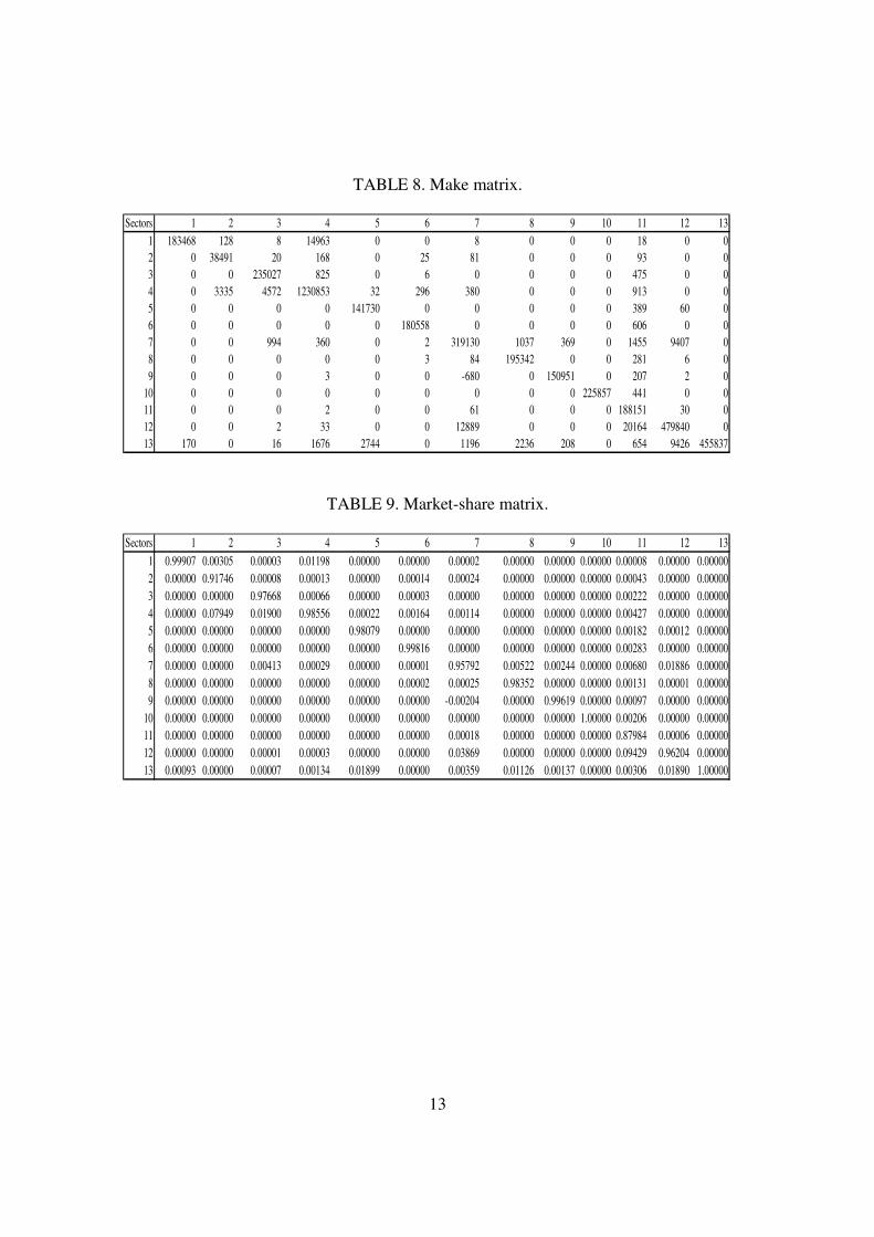
In particular, one of the limitations is important here. The classification problem
presented in the early version of the Leontief model is solved through the pre-multiplication
of the final demand vector, fn, and intersectoral impact matrix, Bn, by the market-share
matrix, D. For instance, doing the market-share table times the Use table (D x Un) creates a
sector by sector Use matrix. In addition, the technology of the sector is assumed in order to
obtain an activity by activity I-O matrix. That is, it assumes that a sector uses the same
3Problem related with the fact that the A matrix in Leontief's model is not a square matrix but instead it is a
commodity by activity matrix. In other words, sectors actually produce and sell a variety of commodities. 4Two different goods produced simultaneously by the same productive process.
5Specific productive processes and chemical reactions of some economic activities may generate secondary
commodities. These commodities are called by-products. For instance, methane gas (CH4) is a by-product of a
chemical reaction that occurs on landfills.

8
technology to produce all their goods.
The Input-Output table for Brazil is aggregated into 13 sectors.6 Because we do not
have the I-O table for 2006, the Input-Output table was derived from national accounting
statistics for 2006. The Resources and Uses table provides the complete information needed
to construct the I-O table. Furthermore, the data for the Value-Added table and Use of Output
table also come from the Resources and Uses table. Lastly, the transfer of funds among
institutions is derived from the Flow of Funds table. The same methodology developed by
Grijó and Berni (2006) is used. In the next section, the steps to build the I-O table and other
results are revealed.
3 THE COMPLETE METHODOLOGY TO ESTIMATE A
SAM FOR BRAZIL
This section describes the methodology used to estimate the SAM for Brazil in 2006.
Subsection 3.1 explores the procedures to calculate the I-O table, including the estimation of
the main matrices from the previous section. Subsection 3.2 presents the treatment to
separate formal and informal activities. Subsection 3.3 presents the two-sector SAM for
Brazil. In the appendix, the procedures to calculate some entries of the FOF table, table that
reveals the flow of income among institutions, are presented.
3.1 From the National Statistical Accounts to the Input-Output Matrix
The methodology to estimate the Input-Output matrix follows the methodology developed by
Guilhoto and Sesso (2002) to build an I-O matrix using national accounting data. According
to this work, the tables presented in the previous section (the net tax, the imports, the import
tax, the transport and trade margins tables) were estimated and deducted from both
Intermediate Use of Output and Final Demand tables. It was needed to convert these two
tables into approximately basic prices. In this subsection, we present the procedure of
estimation of these tables, including the I-O table. In this sense, the transport and trade
margins tables are deducted exclusively from the Intermediate Use of Output table while
6
These sectors are: agriculture, hunting, forestry and fishing; energy sector, mining and quarrying,
manufacturing, public services, construction, wholesale and retail trade, transport and communication,
information service, insurance, real estate, other services, and public administration.
9
other important tables such as tax and imports matrices are deducted from both Intermediate
Use of Output (Use) and Final Demand matrices.
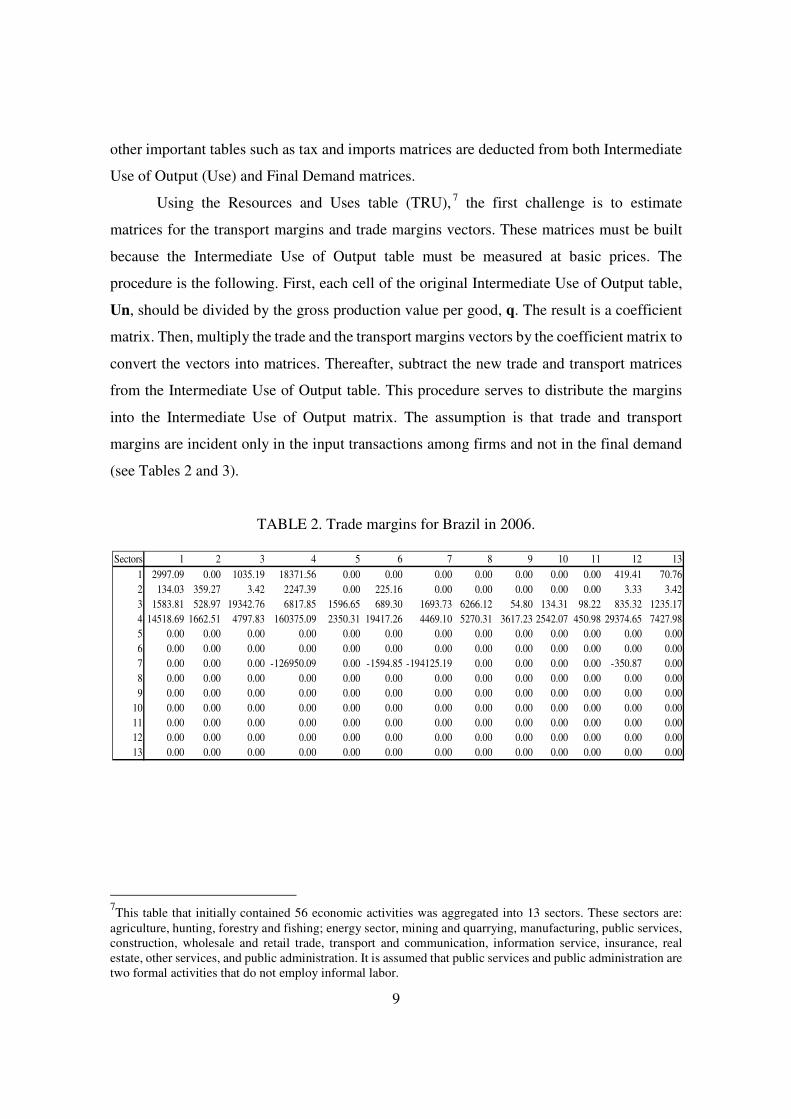
Using the Resources and Uses table (TRU), 7 the first challenge is to estimate
matrices for the transport margins and trade margins vectors. These matrices must be built
because the Intermediate Use of Output table must be measured at basic prices. The
procedure is the following. First, each cell of the original Intermediate Use of Output table,
Un, should be divided by the gross production value per good, q. The result is a coefficient
matrix. Then, multiply the trade and the transport margins vectors by the coefficient matrix to
convert the vectors into matrices. Thereafter, subtract the new trade and transport matrices
from the Intermediate Use of Output table. This procedure serves to distribute the margins
into the Intermediate Use of Output matrix. The assumption is that trade and transport
margins are incident only in the input transactions among firms and not in the final demand
(see Tables 2 and 3).
TABLE 2. Trade margins for Brazil in 2006.
7This table that initially contained 56 economic activities was aggregated into 13 sectors. These sectors are:
agriculture, hunting, forestry and fishing; energy sector, mining and quarrying, manufacturing, public services,
construction, wholesale and retail trade, transport and communication, information service, insurance, real
estate, other services, and public administration. It is assumed that public services and public administration are
two formal activities that do not employ informal labor.
Sectors 1 2 3 4 5 6 7 8 9 10 11 12 13
1 2997.09 0.00 1035.19 18371.56 0.00 0.00 0.00 0.00 0.00 0.00 0.00 419.41 70.76
2 134.03 359.27 3.42 2247.39 0.00 225.16 0.00 0.00 0.00 0.00 0.00 3.33 3.42
3 1583.81 528.97 19342.76 6817.85 1596.65 689.30 1693.73 6266.12 54.80 134.31 98.22 835.32 1235.17
4 14518.69 1662.51 4797.83 160375.09 2350.31 19417.26 4469.10 5270.31 3617.23 2542.07 450.98 29374.65 7427.98
5 0.00 0.00 0.00 0.00 0.00 0.00 0.00 0.00 0.00 0.00 0.00 0.00 0.00
6 0.00 0.00 0.00 0.00 0.00 0.00 0.00 0.00 0.00 0.00 0.00 0.00 0.00
7 0.00 0.00 0.00 -126950.09 0.00 -1594.85 -194125.19 0.00 0.00 0.00 0.00 -350.87 0.00
8 0.00 0.00 0.00 0.00 0.00 0.00 0.00 0.00 0.00 0.00 0.00 0.00 0.00
9 0.00 0.00 0.00 0.00 0.00 0.00 0.00 0.00 0.00 0.00 0.00 0.00 0.00
10 0.00 0.00 0.00 0.00 0.00 0.00 0.00 0.00 0.00 0.00 0.00 0.00 0.00
11 0.00 0.00 0.00 0.00 0.00 0.00 0.00 0.00 0.00 0.00 0.00 0.00 0.00
12 0.00 0.00 0.00 0.00 0.00 0.00 0.00 0.00 0.00 0.00 0.00 0.00 0.00
13 0.00 0.00 0.00 0.00 0.00 0.00 0.00 0.00 0.00 0.00 0.00 0.00 0.00

10
TABLE 3. Transport margins for Brazil in 2006.
The procedure to estimate the matrix for net taxes is the following. Each cell of the
Intermediate Use of Output table must be divided by the total demand vector. The outcome of
this computation is a new coefficient matrix. This new matrix is multiplied by the vector of
net taxes to convert it into matrix.
However, the remaining two matrices, imports and import tax matrices, are estimated
differently. It is necessary to use a different approach because there is no incidence of
imports and imports' taxes in at least one of the final demand components. Imports and
imports' taxes should not be deducted from exports. To solve this problem, two specific
coefficient matrices are calculated to spread both imports and imports' taxes vectors into the
Use and Final Demand matrices.
In this way, the coefficient matrix for the Use table is calculated in two steps. First,
the deduction of the exports from the total demand is necessary. Second, each cell of the Use
table is divided by the total demand vector (without exports) to get a coefficient matrix that
later will be applied to spread imports and import tax into the Intermediate Use of Output
(Use) table. Then, the multiplication of the new coefficient matrix by imports and import tax
vectors gives the imports and import tax matrices. In short, the five matrices (taxes, trade,
transport, imports and imports' taxes) are deducted from the Intermediate Use of Output table
to convert this table into basic prices.
A Similar procedure is applied into the Final Demand table. More specifically, to
estimate the tax matrix, each cell of the final demand matrix is divided by the total demand
Sectors 1 2 3 4 5 6 7 8 9 10 11 12 13
1 328.33 0.00 113.40 2012.57 0.00 0.00 0.00 0.00 0.00 0.00 0.00 45.95 7.75
2 166.72 446.91 4.25 2795.64 0.00 280.08 0.00 0.00 0.00 0.00 0.00 4.14 4.25
3 129.33 43.20 1579.52 556.74 130.38 56.29 138.31 511.69 4.47 10.97 8.02 68.21 100.86
4 1542.83 176.67 509.84 17042.29 249.76 2063.38 474.91 560.05 384.39 270.13 47.92 3121.50 789.34
5 0.00 0.00 0.00 0.00 0.00 0.00 0.00 0.00 0.00 0.00 0.00 0.00 0.00
6 0.00 0.00 0.00 0.00 0.00 0.00 0.00 0.00 0.00 0.00 0.00 0.00 0.00
7 0.00 0.00 0.00 0.00 0.00 0.00 0.00 0.00 0.00 0.00 0.00 0.00 0.00
8 -984.61 -1344.67 -3687.06 -12427.80 -764.04 -378.83 -5621.58 -5483.85 -1137.20 -752.00 -94.88 -2932.58 -1171.90
9 0.00 0.00 0.00 0.00 0.00 0.00 0.00 0.00 0.00 0.00 0.00 0.00 0.00
10 0.00 0.00 0.00 0.00 0.00 0.00 0.00 0.00 0.00 0.00 0.00 0.00 0.00
11 0.00 0.00 0.00 0.00 0.00 0.00 0.00 0.00 0.00 0.00 0.00 0.00 0.00
12 0.00 0.00 0.00 0.00 0.00 0.00 0.00 0.00 0.00 0.00 0.00 0.00 0.00
13 0.00 0.00 0.00 0.00 0.00 0.00 0.00 0.00 0.00 0.00 0.00 0.00 0.00

11
vector. Consequently, the multiplication of the tax vector by the resulting coefficient matrix
produces the tax matrix.
For the same reasons explained previously, the procedure to estimate the remaining
matrices is more complex. This time, the coefficient matrix for the Final Demand table is
calculated in three steps. Firstly, the deduction of the exports from the total demand is again a
necessity. Secondly, the new coefficient matrix must have the whole cells of the column of
exports equal zero. Thirdly, each cell of the Final Demand table (deducted of exports) is
divided by the total demand vector, a vector that does not include exports, to get a coefficient
matrix to spread imports and imports' taxes into the Final Demand matrix. As a result, the
simple multiplication of the coefficient matrix by imports and imports' taxes vectors creates
the imports and imports' taxes matrices. For more details, see Tables 4-10.
TABLE 4. Coefficient matrix.
Sectors 1 2 3 4 5 6 7 8 9 10 11 12 13
1 0.0859 0.0000 0.0297 0.5268 0.0000 0.0000 0.0000 0.0000 0.0000 0.0000 0.0000 0.0120 0.0020
2 0.0266 0.0713 0.0007 0.4461 0.0000 0.0447 0.0000 0.0000 0.0000 0.0000 0.0000 0.0007 0.0007
3 0.0277 0.0093 0.3388 0.1194 0.0280 0.0121 0.0297 0.1097 0.0010 0.0024 0.0017 0.0146 0.0216
4 0.0264 0.0030 0.0087 0.2921 0.0043 0.0354 0.0081 0.0096 0.0066 0.0046 0.0008 0.0535 0.0135
5 0.0087 0.0081 0.0245 0.2268 0.1899 0.0029 0.0432 0.0172 0.0127 0.0105 0.0015 0.0836 0.0602
6 0.0000 0.0000 0.0090 0.0086 0.0000 0.0196 0.0010 0.0002 0.0035 0.0062 0.0239 0.0163 0.0638
7 0.0000 0.0000 0.0000 0.3255 0.0000 0.0041 0.4977 0.0000 0.0000 0.0000 0.0000 0.0009 0.0000
8 0.0155 0.0211 0.0579 0.1953 0.0120 0.0060 0.0883 0.0862 0.0179 0.0118 0.0015 0.0461 0.0184
9 0.0036 0.0071 0.0189 0.0835 0.0100 0.0026 0.0280 0.0126 0.1543 0.0817 0.0027 0.1910 0.1244
10 0.0076 0.0071 0.0075 0.1394 0.0098 0.0078 0.0333 0.0201 0.0179 0.1249 0.0038 0.0241 0.1374
11 0.0010 0.0016 0.0257 0.0314 0.0021 0.0025 0.0452 0.0084 0.0212 0.0068 0.0036 0.0374 0.0385
12 0.0001 0.0030 0.0188 0.0550 0.0127 0.0068 0.0362 0.0233 0.0293 0.0325 0.0050 0.0610 0.0686
13 0.0000 0.0000 0.0000 0.0000 0.0000 0.0000 0.0000 0.0000 0.0000 0.0000 0.0000 0.0000 0.0000

12
TABLE 5. Net taxes.
TABLE 6. Imports for Brazil in 2006.
TABLE 7. Taxes on imports for Brazil for year 2006.
Sectors 1 2 3 4 5 6 7 8 9 10 11 12 13
1 799.23 0.00 276.05 4899.14 0.00 0.00 0.00 0.00 0.00 0.00 0.00 111.84 18.87
2 53.15 142.48 1.35 891.26 0.00 89.29 0.00 0.00 0.00 0.00 0.00 1.32 1.35
3 833.82 278.48 10183.29 3589.36 840.58 362.89 891.69 3298.89 28.85 70.71 51.71 439.77 650.28
4 4126.95 472.57 1363.79 45586.74 668.08 5519.37 1270.35 1498.09 1028.20 722.59 128.19 8349.76 2111.41
5 281.21 264.23 794.85 7356.85 6157.26 92.83 1399.53 556.45 412.33 342.07 49.13 2710.91 1951.46
6 0.00 0.03 50.80 48.29 0.27 110.49 5.40 1.15 19.82 34.93 134.84 91.58 359.53
7 0.00 0.00 0.00 0.00 0.00 0.00 0.00 0.00 0.00 0.00 0.00 0.00 0.00
8 184.73 252.28 691.75 2331.66 143.35 71.08 1054.70 1028.86 213.36 141.09 17.80 550.20 219.87
9 121.29 235.23 628.27 2776.99 331.53 87.56 931.14 420.48 5136.29 2720.19 88.43 6357.18 4139.44
10 98.06 92.29 96.51 1802.86 126.29 100.47 430.90 259.91 231.52 1615.29 48.87 311.46 1776.07
11 1.52 2.45 39.60 48.42 3.20 3.92 69.67 12.95 32.65 10.53 5.48 57.75 59.33
12 3.71 89.42 566.10 1654.25 380.77 205.20 1089.57 700.94 880.59 977.87 148.92 1832.37 2060.67
13 0.00 0.00 0.00 0.00 0.00 0.00 0.00 0.00 0.00 0.00 0.00 0.00 0.00
Sectors 1 2 3 4 5 6 7 8 9 10 11 12 13
1 505.58 0.00 174.63 3099.12 0.00 0.00 0.00 0.00 0.00 0.00 0.00 70.75 11.94
2 418.11 1120.76 10.65 7010.91 0.00 702.39 0.00 0.00 0.00 0.00 0.00 10.39 10.65
3 1104.19 368.78 13485.25 4753.22 1113.14 480.56 1180.82 4368.57 38.20 93.64 68.47 582.36 861.13
4 4981.58 570.43 1646.21 55027.13 806.43 6662.36 1533.42 1808.32 1241.13 872.22 154.74 10078.89 2548.65
5 22.84 21.46 64.55 597.49 500.07 7.54 113.66 45.19 33.49 27.78 3.99 220.17 158.49
6 0.00 0.00 1.99 1.90 0.01 4.34 0.21 0.04 0.78 1.37 5.29 3.59 14.11
7 0.00 0.00 0.00 825.32 0.00 10.37 1262.03 0.00 0.00 0.00 0.00 2.28 0.00
8 95.53 130.46 357.72 1205.74 74.13 36.75 545.40 532.04 110.33 72.96 9.21 284.52 113.70
9 20.53 39.81 106.34 470.02 56.11 14.82 157.60 71.17 869.34 460.40 14.97 1075.98 700.62
10 23.08 21.73 22.72 424.41 29.73 23.65 101.44 61.19 54.50 380.25 11.50 73.32 418.10
11 13.11 21.16 341.92 418.10 27.63 33.81 601.54 111.80 281.94 90.93 47.33 498.66 512.30
12 2.83 68.14 431.42 1260.68 290.18 156.38 830.34 534.18 671.09 745.23 113.49 1396.43 1570.41
13 0.00 0.00 0.00 0.00 0.00 0.00 0.00 0.00 0.00 0.00 0.00 0.00 0.00
Sectors 1 2 3 4 5 6 7 8 9 10 11 12 13
1 9.34 0.00 3.23 57.28 0.00 0.00 0.00 0.00 0.00 0.00 0.00 1.31 0.22
2 0.51 1.37 0.01 8.55 0.00 0.86 0.00 0.00 0.00 0.00 0.00 0.01 0.01
3 0.34 0.11 4.10 1.44 0.34 0.15 0.36 1.33 0.01 0.03 0.02 0.18 0.26
4 291.58 33.39 96.36 3220.82 47.20 389.96 89.75 105.84 72.64 51.05 9.06 589.93 149.18
5 0.00 0.00 0.00 0.00 0.00 0.00 0.00 0.00 0.00 0.00 0.00 0.00 0.00
6 0.00 0.00 0.00 0.00 0.00 0.00 0.00 0.00 0.00 0.00 0.00 0.00 0.00
7 0.00 0.00 0.00 0.00 0.00 0.00 0.00 0.00 0.00 0.00 0.00 0.00 0.00
8 0.00 0.00 0.00 0.00 0.00 0.00 0.00 0.00 0.00 0.00 0.00 0.00 0.00
9 0.00 0.00 0.00 0.00 0.00 0.00 0.00 0.00 0.00 0.00 0.00 0.00 0.00
10 0.00 0.00 0.00 0.00 0.00 0.00 0.00 0.00 0.00 0.00 0.00 0.00 0.00
11 0.00 0.00 0.00 0.00 0.00 0.00 0.00 0.00 0.00 0.00 0.00 0.00 0.00
12 0.00 0.00 0.00 0.00 0.00 0.00 0.00 0.00 0.00 0.00 0.00 0.00 0.00
13 0.00 0.00 0.00 0.00 0.00 0.00 0.00 0.00 0.00 0.00 0.00 0.00 0.00
13
TABLE 8. Make matrix.
TABLE 9. Market-share matrix.
Sectors 1 2 3 4 5 6 7 8 9 10 11 12 13
1 183468 128 8 14963 0 0 8 0 0 0 18 0 0
2 0 38491 20 168 0 25 81 0 0 0 93 0 0
3 0 0 235027 825 0 6 0 0 0 0 475 0 0
4 0 3335 4572 1230853 32 296 380 0 0 0 913 0 0
5 0 0 0 0 141730 0 0 0 0 0 389 60 0
6 0 0 0 0 0 180558 0 0 0 0 606 0 0
7 0 0 994 360 0 2 319130 1037 369 0 1455 9407 0
8 0 0 0 0 0 3 84 195342 0 0 281 6 0
9 0 0 0 3 0 0 -680 0 150951 0 207 2 0
10 0 0 0 0 0 0 0 0 0 225857 441 0 0
11 0 0 0 2 0 0 61 0 0 0 188151 30 0
12 0 0 2 33 0 0 12889 0 0 0 20164 479840 0
13 170 0 16 1676 2744 0 1196 2236 208 0 654 9426 455837
Sectors 1 2 3 4 5 6 7 8 9 10 11 12 13
1 0.99907 0.00305 0.00003 0.01198 0.00000 0.00000 0.00002 0.00000 0.00000 0.00000 0.00008 0.00000 0.00000
2 0.00000 0.91746 0.00008 0.00013 0.00000 0.00014 0.00024 0.00000 0.00000 0.00000 0.00043 0.00000 0.00000
3 0.00000 0.00000 0.97668 0.00066 0.00000 0.00003 0.00000 0.00000 0.00000 0.00000 0.00222 0.00000 0.00000
4 0.00000 0.07949 0.01900 0.98556 0.00022 0.00164 0.00114 0.00000 0.00000 0.00000 0.00427 0.00000 0.00000
5 0.00000 0.00000 0.00000 0.00000 0.98079 0.00000 0.00000 0.00000 0.00000 0.00000 0.00182 0.00012 0.00000
6 0.00000 0.00000 0.00000 0.00000 0.00000 0.99816 0.00000 0.00000 0.00000 0.00000 0.00283 0.00000 0.00000
7 0.00000 0.00000 0.00413 0.00029 0.00000 0.00001 0.95792 0.00522 0.00244 0.00000 0.00680 0.01886 0.00000
8 0.00000 0.00000 0.00000 0.00000 0.00000 0.00002 0.00025 0.98352 0.00000 0.00000 0.00131 0.00001 0.00000
9 0.00000 0.00000 0.00000 0.00000 0.00000 0.00000 -0.00204 0.00000 0.99619 0.00000 0.00097 0.00000 0.00000
10 0.00000 0.00000 0.00000 0.00000 0.00000 0.00000 0.00000 0.00000 0.00000 1.00000 0.00206 0.00000 0.00000
11 0.00000 0.00000 0.00000 0.00000 0.00000 0.00000 0.00018 0.00000 0.00000 0.00000 0.87984 0.00006 0.00000
12 0.00000 0.00000 0.00001 0.00003 0.00000 0.00000 0.03869 0.00000 0.00000 0.00000 0.09429 0.96204 0.00000
13 0.00093 0.00000 0.00007 0.00134 0.01899 0.00000 0.00359 0.01126 0.00137 0.00000 0.00306 0.01890 1.00000

14
TABLE 10. Use matrix sector by sector for Brazil in 2006 at basic prices.
The Final Demand matrix at approximately basic prices is the result of the final
demand at market prices minus the tax matrix, the imports matrix, and the imports' taxes
matrix. It is a standard procedure to transform the final demand components previously
measured at market prices into basic prices. Table 11 shows the Final Demand matrix (sector
by sector) at approximately basic prices. Furthermore, the components of the Use of Output
part of the SAM (exports, household consumption, government purchases, and capital
accumulation) are the result of these deductions.
TABLE 11. Demand matrix (sector by sector) at approximately basic prices.
Sectors 1 2 3 4 5 6 7 8 9 10 11 12 13
1 14865.16 39.63 5132.17 92554.31 46.46 386.26 93.68 104.58 71.51 50.12 8.94 2618.30 491.12
2 771.24 2057.83 29.41 12940.83 1.22 1294.86 54.12 3.95 2.87 1.39 1.06 29.80 26.76
3 5962.74 1988.60 72641.39 25786.97 5998.29 2610.39 6385.53 23536.34 219.74 510.33 371.08 3185.98 4664.25
4 23666.73 2907.63 9201.62 261199.91 3926.13 31578.75 7622.08 8990.44 5875.47 4129.91 746.98 47617.00 12162.26
5 1229.28 1155.49 3484.66 32165.44 26909.21 407.08 6135.74 2436.39 1811.87 1499.47 216.36 11865.08 8547.07
6 0.60 1.93 1643.76 1566.97 9.96 3543.19 200.41 41.82 648.05 1123.77 4324.08 2958.09 11547.45
7 54.15 66.88 598.63 125636.74 166.17 1661.61 191126.43 439.08 386.29 362.68 56.22 1122.92 790.18
8 3428.19 4681.96 12843.86 43309.42 2660.65 1320.13 19634.61 19094.56 3965.31 2620.22 331.44 10220.81 4091.37
9 550.34 1067.22 2854.86 12336.53 1504.08 394.39 3826.47 1908.87 23299.78 12338.74 401.82 28839.87 18782.30
10 1713.29 1612.69 1697.08 31504.56 2206.89 1756.00 7546.55 4543.60 4053.30 28217.46 855.19 5456.72 31039.77
11 185.13 298.70 4826.04 5926.51 390.30 477.67 8526.91 1578.49 3979.88 1284.26 668.11 7039.44 7232.03
12 79.64 1456.34 9534.71 32021.63 6106.72 3383.69 25961.48 11333.94 14452.54 15713.05 2443.61 29955.15 33597.19
13 111.48 110.23 432.19 2577.99 679.55 138.17 1443.18 506.25 409.64 391.97 58.43 1051.84 924.56
Sectors Exports Government Consumption Investment
1 23661.24 41.71 45267.28 13160.53
2 20091.95 0.47 407.75 1162.48
3 28537.89 2.30 52555.84 1375.35
4 204203.87 3431.29 439574.66 173546.27
5 7.67 1.41 44296.86 9.94
6 920.10 0.00 447.18 152186.62
7 2711.61 222.11 7230.46 121.83
8 4919.27 0.14 62584.46 9.60
9 700.84 0.06 41671.22 5.63
10 1855.73 1553.15 100674.94 11.07
11 2245.53 0.71 138859.64 4724.65
12 24541.68 11278.42 289143.44 1924.76
13 844.67 456063.22 8129.33 290.29

15
The Input-Output matrix at approximately basic prices, therefore, is the result of the
Intermediate Use of Output table at market prices minus the tax matrix, the imports matrix,
the import' tax matrix, trade matrix, and transport matrix. In the Appendix A, one of the
important components of the Social Accounting Matrix (SAM) is presented. Because the
Flow of Funds table, table that measures the flow of income among institutions, is not
directly available, an alternative procedure is implemented. Finally, Sections 3.2 and 3.3
present the process of aggregation of the I-O Matrix and SAM, including the methodology
that distinguishes between the formal and informal sectors.
3.2 Formal and Informal Activities in Brazil
In this study, the informal sector is defined as a subdivision of the household sector in the
System of National Accounts - SNA, characterized by a particular way of organizing the
production and an unclear division between labor and capital. This sector includes businesses
that are not officially registered. Hallak et al. (2009) estimated the size of the informal sector
for the aggregate economy and for 10 sectors from 2000 to 2007. Informal labor has two
main component parts: autonomous labor and employees without legal contract. Moreover, it
is assumed that the informal sector uses only informal labor. To estimate a SAM that
separates between formal and informal activities, the estimations by Hallak et al. (2009) are
used. These estimations for the 10 sectors were disaggregated into 12 sectors following the
procedures suggested by the Brazilian Institute of Geography and Statistics (SNA-IBGE,
2009). Table 12, below, presents the 13 shares (weights) for formal and informal sectors.

16
TABLE 12. Sectoral value-added shares.
The statistics of value added for informal activities for the 12 major sectors in 2007
are employed to estimate the shares of the informal and formal sectors in 2006. It is assumed
that there is no significant structural change, in terms of the change in the size of the informal
sector, between 2006 and 2007. Specifically for agriculture, wage shares for formal and
informal sectors are being applied to separate each transaction into four entries. Equations 15
and 16, below, are applied to estimate the shares for the formal and informal sectors for 12
economic activities. The shares are presented below:
VAFVAI
VAII
+=ϕ (15)
VAFVAI
VAFF
+=ϕ (16)
where Iϕ , Fϕ are the shares (weights) for the informal and formal sectors and VAI , VAF
are the value-added for the informal and formal sectors, respectively.
Further, these sectoral shares of output are being used as weights to calculate the size
of the informal sector. Each recorded transaction in the Input-Output table for the 13
Informal Formal
Agriculture 0.505 0.495
Mining and Quarrying 0.027 0.973
Energy 0.000 1.000
Manufacturing 0.062 0.938
Construction 0.265 0.735
Wholesale and Retail 0.210 0.790
Transport 0.227 0.773
Information Services 0.127 0.873
Financing and Insurance 0.009 0.991
Real Estate 0.016 0.984
Other Services 0.227 0.773
Distribution of electricity 0.000 1.000
Public Administration 0.000 1.000

17
activities will be separated into four entries. This methodology is based in Rada (2010). The
four entries for the transaction of intermediate inputs, jXi, , purchased by sector j from
sector i are presented below:
Formal sector i - Formal sector j:
jFiFjXiFFjXi ,*,*,=, ϕϕ− (17)
Formal Sector i - Informal sector j:
jIiFjXiFIjXi ,*,*,=, ϕϕ− (18)
Informal sector i - Formal sector j:
jFiIjXiIFjXi ,*,*,=, ϕϕ− (19)
Informal sector i - Informal sector j:
jIiIjXiIIjXi ,*,*,=, ϕϕ− (20)
Thereafter, we need to aggregate all the informal sector transactions into a unique
informal sector. A similar procedure is adopted to aggregate the set of formal activities into a
unique formal sector. The result is an Input-Output table, with only two major sectors, that
distinguishes between formal and informal activities.
Slightly different procedure is adopted to separate every transaction in the Use of
Output (Final Demand) quadrant of the SAM. The process to separate households between
formal and informal is different. For agriculture, this study uses the values of the wage share
as weights to divide the consumption between formal and informal households.
To separate the aggregate consumption between the formal and informal for the other
remaining sectors, the procedure adopted is to use the previous shares (Table 12), which
separate the transactions of the I-O table, and a new one that is the percentage of value-added

18
for the economy as a whole. In this way, the share of the value-added for the formal sector is
78.36 percent, while the informal sector is 21.64 percent. That is, the formal sector
represents 78.36 percent of the GDP. The equation below presents the procedure. For
instance, the amount of consumption that the formal household, j, buys from formal
manufacturing, i, is the result of the following equation.
Formal sector i - Household j:
FiFjCiFFjCi φϕ *,*,=, − (21)
where Fφ is the index for the formal sector ( 78.36 percent) and iF ,ϕ is the value-added
share of the formal sector, in this case manufacturing, used previously as weights to separate
informal and formal activities in the Input-Output table. A similar procedure is applied to
separate the consumption between formal and informal households for the other 12 sectors.
Thereafter, it is possible to aggregate in only two sectors and two consumers. The RAS
technique, an algorithm used to balance square matrices, is applied to balance the sum of
rows and columns of the SAM.
The Use of Output quadrant of the SAM has three additional components. First,
exports are assumed to include formal activities only. The value of 315.24 billion reals
represents exports of goods and services together. Next, government purchases are treated as
expenditures on formal goods only. The value of 472.59 billion reals describes the
government consumption for 2006. Finally, it is assumed that capital accumulation takes
place only in the formal sector. The value of 397.03 billion reals, about 16.7 percent of GDP,
reveals a low level of investment compared to other fast-growing emerging economies.
The quadrant below the I-O table provides the sectoral costs, excluding intermediate
inputs, to produce the output being sold. In this quadrant, the wages of formal and informal
labor are presented. Formal workers' remuneration comes directly from national accounting
statistics. This group includes the remuneration of employees with legal contracts such as
civil servants, military workers, etc.
For informal workers, wages are the result of adding autonomous remuneration8 to
wages paid to workers in the informal sector. We assume that the informal sector does not
8Autonomous remuneration consists in the remuneration of own-account workers and informal employers.

19
employ formal workers. The value of 279.73 billion reals comes directly from national
accounting statistics. Profits and wages are put together in the same entry because of the
assumption that there is no clear differentiation between labor remuneration and profits for
the informal sector. Conversely, for the formal sector, there are two distinct entries for profits
and labor remuneration.
Another category of the sectoral costs is the imported inputs. Imported inputs are
assumed to be concentrated into the formal sector, that is, only formal activities are capable
to import inputs from the rest of the world. Lastly, government tax on production has
incidence in the formal sector only. Table 1 shows that the origin of the data comes from the
Resources and Uses table (TRU).
Turning now to the center of the SAM, the entries describe the transfers of funds
among institutions. Because the Brazilian Statistical Office does not release directly the
complete Flow of Funds table, we attempt to estimate the transfers of income among
institutions indirectly. The Integrated Economic Accounts (in Portuguese: Contas
Econômicas Integradas: CEI) provides the main information needed to a reliable estimation
of these entries. This table presents five major institutions: families, government, financial
enterprises, nonfinancial enterprises, and the rest of the world. Some of the entries in the
center of the SAM are: transfer of income from government to workers, income from
properties, rents, dividends and interest paid to workers, capital transfers, final goods
imports, government and business transfers to the rest of the world, capital goods imports,
etc.
There are two major assumptions concerning the numbers in the center of the SAM.
First, transfers from government to households and transfer from capitalist to households are
calculated endogenously.9 Treating transfer as a residual is necessary because of the
inconsistencies between different sources of data. The shares of value-added for formal and
informal activities are applied as weights to separate transfers between formal and informal
workers. Second, informal households do not pay direct (income) tax.
Finally, government savings, capitalist savings, and household savings come from
the same table (CEI) and the same code or transaction, B.12. Moreover, the current account
9
For instance, the government transfer toward labor is the result of subtracting government spending
(excluding transfers) and savings from government revenue.

20
result is derived from transaction B.12 (resources). The complete procedure to calculate the
remaining entries is described in Appendix A.
3.3 A Social Accounting Matrix that Includes Formal and Informal
Sectors
The two-sector SAM for Brazil is presented in Table 13. The Input-Output table is located in
the northwest corner of the SAM. Equations 17-20 were applied to calculate the I-O table.
The formal sector provides inputs to the informal sector in the amount of 169.53 billion
Brazilian reals (column B), and provides intermediate goods worth 1,334 billion reals to
itself (column A).
TABLE 13. Social accounting matrix for Brazil for year 2006.
Formal households purchase final goods from the formal sector in the amount of
722.43 billion reals while informal households consume only 275.46 billion reals. Using the
classical assumption that capitalist consumption is not significant, the capitalists'
consumption is zero (column D).
The amount of 315.24 billion reals (column G) represents the demand from the rest of
the world while investment goods (column H) are estimated at 348.53 billion reals. If
compared to imports (row 7, column A), equivalent to 153.87 billion reals, the Brazilian
economy has a trade surplus in the period. The total output (column I) for the formal sector is
estimated at 3,637.89 billion reals. If we add the first row of the I-O table to the first row of
SAM 2006
(billion of reals) Formal
(A)
Informal
(B)
Formal HH
( C)
Business
(D)
Informal HH
(E)
Government
(F)
Exports
(G)
(1) Formal (F) 1334.10 169.53 722.43 275.46 472.59 315.24 348.53 3637.89
(2) Informal (I) 216.31 30.97 162.05 70.89 480.23
(3) Labor (F) 902.58 221.54 66.12 0.39 1190.63
(4) Business (F) 825.00 825.00
(5) Labor (I) 279.73 61.02 18.24 358.99
(6) Government 206.03 110.61 138.74 176.63 25.21 25.03 682.25
(7) Imports 153.87 93.35 35.60 15.00 23.47 321.29
(8) Savings 102.18 368.10 12.63 -66.33 -19.56 -397.03 0.00
(9) Totals 3637.89 480.23 1190.63 825.00 358.99 682.25 321.29
Costs Use of Income
Investment
(H)
Totals
(I)

21
the components of the final demand, the total output value can be calculated.
Turning now to the informal sector, similar interpretation can be made. Overall, this
sector total output is estimated at 480.23 billion reals. Similar result can be found if we add
the Input-Output table (column B) to the cost components (informal compensation). Informal
labor compensation captures 279.73 billion reals of the informal sector's output.
Finally, the Flow of Funds table, in the center of the SAM, presents some interesting
entries. Formal workers receive wages (column A), transfers from business (dividends, and
payment of interest) and government transfers. The total income of formal workers is
estimated at 1,190.63 billion reals. In column C, the income of formal household is being
spent on 884.48 billion reals of final consumption goods from both sectors.
Informal workers receive wages (column B), transfers from business (dividends, and
payment of interest) and government transfers. The total income of informal workers is
estimated at 358.99 billion reals. In column E, the income of informal households is being
spent on 346.35 billion reals of final consumption goods from both sectors. From this
amount, purchases from the informal sector capture 70.89 billion reals, or 20.46 percent of
formal household's final demand. For the remaining institutions, other entries can be read in
similar fashion.
The results suggest that the informal sector has an important role in the Brazilian
economy. Economic policies that intend to reduce poverty and create employment must
consider the importance of this sector to the whole economy and its structural relationship
with the formal sector.
4 CONCLUSIONS
The analyses of the SAM and its components reveal the importance of the informal sector
and the relative degree of structural interdependence of the Brazilian economy. Table 14
illustrates important statistics for the two sectors for Brazil in 2006.
22
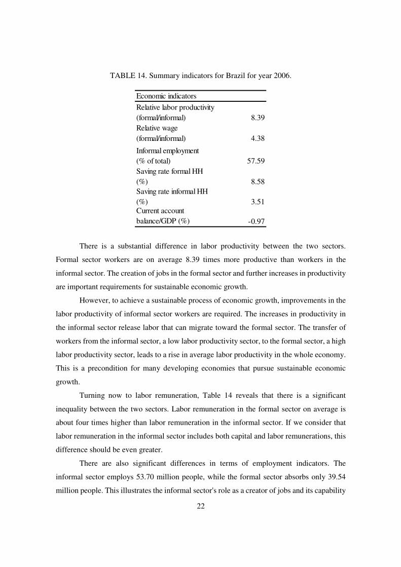
TABLE 14. Summary indicators for Brazil for year 2006.
There is a substantial difference in labor productivity between the two sectors.
Formal sector workers are on average 8.39 times more productive than workers in the
informal sector. The creation of jobs in the formal sector and further increases in productivity
are important requirements for sustainable economic growth.
However, to achieve a sustainable process of economic growth, improvements in the
labor productivity of informal sector workers are required. The increases in productivity in
the informal sector release labor that can migrate toward the formal sector. The transfer of
workers from the informal sector, a low labor productivity sector, to the formal sector, a high
labor productivity sector, leads to a rise in average labor productivity in the whole economy.
This is a precondition for many developing economies that pursue sustainable economic
growth.
Turning now to labor remuneration, Table 14 reveals that there is a significant
inequality between the two sectors. Labor remuneration in the formal sector on average is
about four times higher than labor remuneration in the informal sector. If we consider that
labor remuneration in the informal sector includes both capital and labor remunerations, this
difference should be even greater.
There are also significant differences in terms of employment indicators. The
informal sector employs 53.70 million people, while the formal sector absorbs only 39.54
million people. This illustrates the informal sector's role as a creator of jobs and its capability
Economic indicators
Relative labor productivity
(formal/informal) 8.39
Relative wage
(formal/informal) 4.38
Informal employment
(% of total) 57.59
Saving rate formal HH
(%) 8.58
Saving rate informal HH
(%) 3.51Current account
balance/GDP (%) -0.97

23
to absorb surplus labor.
Additionally, it is interesting to make an in-depth analysis of the structural linkages
between the two sectors. Table 15 provides the Leontief inverse matrix. The formal sector
has the largest impact on the economy through its overall multiplier of 1.74. It means that a
unit of increase in the demand of the formal sector good causes the total output to increase
1.74 units. The informal sector has a slightly lower impact on the economy; its overall
multiplier is 1.72. These results suggest that policies that intend to improve economic activity
should focus on stimulating demand in both sectors. However, the overall impact of the
informal sector on the economy might be overestimated because of the aggregation of
heterogeneous subsectors into the informal sector. Rada (2010) points out that further efforts
should be made to estimate structural linkages between the formal sector and specific
informal subsectors.
TABLE 15. The Leontief inverse matrix.
Analyzing the other elements of the Leontief inverse matrix, we can see that the
elements of its main diagonal, as expected, are larger than one. The off-diagonal elements,
measures of backward linkages between the two sectors, suggest that the informal sector is
highly dependent on formal sector provisions of intermediate goods. To satisfy a unit of
increase in the demand of the informal commodity, the informal sector needs to demand 0.61
units from the formal sector's good. On the other hand, the formal sector is not very
dependent from the informal sector's goods. The formal sector only needs 0.10 units from the
informal sector's goods in response to an increase of a unit in its own demand.
To improve economic conditions and stimulate sustainable economic expansion,
policies that focus on formal and informal sectors are required. The SAM and its multipliers
suggest that the informal sector is important in the Brazilian economy as a generator of jobs
and a strategic sector to absorb labor during economic downturns. Policies that try to increase
labor productivity in the informal sector are relevant to boost economic growth. Any
Sectors 1 2
(1) Formal 1.637 0.618
(2) Informal 0.104 1.108
Multiplier 1.741 1.726

24
policy-driven Structuralist Calibrated model, therefore, should consider the intrinsic
relationship between the two sectors and the major role that the informal sector has in the
process of economic growth.
References
Berni, D. and V. Lautert (2011) Mesoeconomia: Lições de Contabilidade Social. Porto
Alegre, Bookman.
Grijó, E. and D. Berni (2006) A Metodologia Completa para a Estimativa de Matrizes de
Insumo-Produto. Teoria e Evidência Empírica, 14, 9–42.
Guilhoto, J. J. M., U. A. Sesso (2005) Estimação da Matriz Insumo-Produto a Partir de Dados
Preliminares das Contas Nacionais. Economia Aplicada, 9, 1–23.
Hallak, João, Katia Namir, K., and Luciene Kozovits. 2009. “Setor e Emprego Informal no
Brazil: Analise dos Resultados da Nova Serie do Sistema de Contas Nacionais
2000/2007.” Anais do XXXVIII Encontro Nacional de Economia.
http://www.anpec.org.br/encontro2010 (accessed 9 June 2009).
Instituto Brasileiro de Geografia e Estatística (IBGE). 1994–2009. “Tabela de Recursos e
Usos.” Governo Federal.
http://www.ibge.gov.br/home/estatistica/economia/contasnacionais/2009
(accessed 8 September 2010).
Jorgenson, D. W. (1961) The Development of a Dual Economy. The Economic Journal, 71,
309–334.
Jorgenson, D. W. (1967) Surplus Agricultural Labor and the Development of a Dual
Economy. Oxford University Papers, 19, 288–312.
Leontief, W. (1986) Input-Output Economics. New York, Oxford University Press.
Lewis, W. A. (1954) Economic Development with Unlimited Supplies of Labour.
Manchester School, 28, 139–191.
Miller, R. E. and P. D. Blair (1985) Input-Output Analysis: Foundations and Extensions.
Englewood Cliffs, Prentice-Hall.
Pyatt, G. (1988) A SAM Approach to Modeling. Journal of Policy Modeling, 10, 327–352.
Pyatt, G. (1991) Fundamentals of Social Accounting. Economic Systems Research, 3,
129–153.
Rada, C. (2007) Stagnation or Transformation of a Dual Economy through Endogenous
Productivity Growth. Cambridge Journal of Economics, 31, 711–740.
Rada, C. (2010) Formal and Informal Sectors in China and India. Economic Systems
Research, 22, 315–341.
Ros, J. (2000) Development and the Economics of Growth. Ann Arbor, The University of
Michigan Press.
Taylor L. (1979) Macro Models for Developing Countries. New York, McGraw-Hill.
Taylor, L. (1983) Structuralist Macroeconomics: Applicable Models for the Third World.
New York, Basic Books.
Thomas, V. B. (1982) Input-output Analysis in Developing Countries: Sources, Methods and
Applications. John Wiley and Sons Ltd.

25
APPENDIX A: THE FLOW OF FUNDS TABLE
Because the Brazilian Statistical Office does not directly release the complete Flow of Funds
table, we attempt to estimate the transfers of resources among institutions indirectly. The
Integrated Economic Accounts (CEI) in 2006 provides the main information needed to a
reliable estimation of the transfers of income among institutions. This table presents five
major institutions: families, government, financial enterprises, nonfinancial enterprises, and
the rest of the world (ROW). The Flow of Funds table is the source of data to build the
quadrant in the center of the SAM. Some of the entries in the center of the SAM are: transfer
of income from government to workers, income from properties, rents, dividends and interest
paid to workers, capital transfers, final goods imports, government and business transfers to
the rest of the world , capital goods imports, etc.
To find the values of the cells in the secondary distribution of income of the SAM,
this study looked at the transactions among the five institutions. First, transfers from
government to households and transfers from capitalist to households are endogenous.
Treating transfers as a residual was necessary because of the inconsistencies between the
sources of data. The shares of value-added for formal and informal activities were applied as
weights to separate transfers between formal and informal workers. Second, informal
households do not pay income tax. Third, government savings, capitalist savings, and
household savings come from the same table, code/transaction B.12. Moreover, the current
account result is derived from the transaction B.12 (resources) in the account rest of the
world.
The next scalar is the vector of direct tax paid by families. Its value is obtained from
transaction D.5, income tax, in the account uses of family (S.14) plus 177 million reals
(direct tax paid by nonprofit firms). Its value is 81,950 million plus 177 that is equal to
82,127 million reals. Households pay direct and indirect taxes, therefore, the additional
values of indirect tax is added. The indirect tax values come from our estimations of the
Input-Output matrix.
Another important scalar is the net remuneration of employees received from the rest
of the world. It is the result of transaction D.1 (uses, rest of world), 864, minus transaction
D.1 (resources, rest of world), 475.

26
The scalar of direct tax paid by firms, including financial and nonfinancial firms, is
obtained from transaction D.5, income tax, in the left side of the CEI (Uses). The value of
138,740 million reals was obtained adding the rubric S.11 (firms), 14,639 million reals, and
account S.12 (nonfinancial firms) with the value of 124101 million reals.
The scalar of imports follows the same procedure to calculate the indirect tax. It
comes from the estimations of the Input-Output Matrix. Imports are separated among three
purposes: imports of final goods, imports of inputs and imports of capital goods.
However, the task to estimate the scalars rmc, 35.60 billion reals, and rmg, 14.01
billion reals, is more cumbersome. The scalars rmc and rmg stand for the net transfer of
property income from business to the rest of the world and net transfer of income from
government to rest of the world, respectively.
Table 16 shows the gross transfers between institutions. The task is to calculate net
results to get rmc and rmg. The transactions D.4 represents the total income from property
(D.4=D.41+D.42+D.43+D.44+D.45). D.41 represents the interest rate paid. D.45 represents
the remuneration of land while D.7 represents other transfers.
The next step is to calculate the net transfers. For instance, government in the
transaction D.41 is the only net transfer institution. It sends 144.610 billion (Table 18),
248.630 minus 104.03 (in Table 16), to firms, families and rest of the world. The same
procedure is used to calculate net transfers for each institution.
Finally, the government and firms are the two institutions that make net transfer to
families and the rest of world. In Table 19, the scalars rmc and rmg are presented. The net
transfer from government to the rest of world is the result of adding the values in the
government column. The same process is applied to calculate the net transfer of property
income from business to the rest of the world. The scalars rmc and rmg assume, respectively,
the values of 35.60 and 14.01. To find out the total amount that government send to rest of
world, the amount of government imports must be added.

27
TABLE 16. Economic transfers among institutions (billions of reals).
TABLE 17. Economic transfers among institutions (billions of reals).
TABLE 18. Economic transfers among institutions (billions of reals).
Total ROW Families Government Business Business Government Families ROW Total
1507.29 14.47 66.87 248.63 1177.32 D.4 1069.87 135.04 228.94 73.45 1507.29
12.38 66.73 248.63 931.93 D.41 996.81 104.03 123.08 35.76
2.09 183.10 D.42 70.97 10.64 65.88 37.69
42.19 D.44 2.09 0.13 39.97
0.14 20.11 D.45 20.25
286.11 10.54 28.42 206.01 41.13 D.7 28.99 208.60 47.34 1.18 286.11
5.62 0.09 3.35 D.71 9.06
9.06 D.72 3.30 0.03 5.73
10.35 22.81 18.01 26.04 D.75 4.76 29.93 41.60 0.91
40.72 15.90 24.82 D.8 40.72 40.72
1834.12 25.01 95.30 470.54 1243.27 TOTAL 1098.86 343.65 316.99 74.62 1834.12
271.30 126.89 144.41 NET RESULT 221.69 49.61 271.30
USES
Code/Transaction
RESOURCES
Total ROW Families Government Business Business Government Families ROW Total
12.38 66.73 248.63 931.93 D.41 996.81 104.03 123.08 35.76
2.09 183.10 D.42 70.97 10.64 65.88 37.69
42.19 D.44 2.09 0.13 39.97
0.14 20.11 D.45 20.25
5.62 0.09 3.35 D.71 9.06
9.06 D.72 3.30 0.03 5.73
10.35 22.81 18.01 26.04 D.75 4.76 29.93 41.60 0.91
USES
Code/Transaction
RESOURCES
Total ROW Families Government Business Business Government Families ROW Total
144.61 D.41 64.89 56.35 23.37
112.13 D.42 10.64 35.60
40.10 D.44 0.13 39.97
0.14 20.11 D.45 20.25
5.62 0.09 D.71 5.71
5.76 D.72 0.03 5.73
0.08 D.74 0.08
9.44 21.27 D.75 11.92 18.80
USES
Code/Transaction
RESOURCES

28
TABLE 19. Economic transfers among institutions (billions of reals).
Total Government Business ROW Total
23.37 23.37 D.41 23.37 23.37
35.60 35.60 D.42 35.60 35.60
D.71
D.72
0.08 0.08 D.74 0.08 0.08
-9.44 -9.44 D.75 -9.44 -9.44
49.61 14.01 35.60
Net income transfer to rest
of the world 49.61 49.61
USES
CODE / TRANSACTION
RESOURCES