Department of Mathematical Economics and Economy Analysis Department of Finance

THESIS OUTLINE

Zita Marossy

Analysis of spot electricity prices using statistical and econophysical methods

submitted for the degree of a Ph.D.

Supervisor:

Dr. Imre Csekő Ph.D. Associate professor

© Zita Marossy

Contents

BRIEF LITERATURE SUMMARY AND AIM OF RESEARCH.................................................... 5

METHODOLOGY ................................................................................................................................. 9

THESES ................................................................................................................................................. 20

HYPOTHESIS 1...................................................................................................................................... 20

HYPOTHESIS 2...................................................................................................................................... 23

HYPOTHESIS 3...................................................................................................................................... 23

HYPOTHESIS 4...................................................................................................................................... 25

HYPOTHESIS 5...................................................................................................................................... 26

HYPOTHESIS 6...................................................................................................................................... 30

HYPOTHESIS 7...................................................................................................................................... 32

EMPIRICAL MODEL ............................................................................................................................... 34

CONCLUSIONS ................................................................................................................................... 35

SELECTED BIBLIOGRAPHY........................................................................................................... 38

OWN PUBLICATIONS IN THE RESEARCH FIELD OF THE THESIS .................................... 40

4

5

Brief literature summary and aim of research

Due to the liberalization and deregulation of electricity markets, we are witnessing the

appearance of organized markets in many countries. One form of these organized markets is the

electricity exchange (e.g. EEX, Nord Pool, APX) where day-ahead electricity is traded and one can

bid on power supplied during the next day or weekday or during one hour, peak hours, or off-peak

hours of the following day. Market participants make their buy or sell bids on the electricity of the

given period and the exchange constructs a market supply and demand curve. The intersection of

the market supply and demand curve will produce the market clearing price (MCP) which generally

equals to the spot price of that period (Weron [2006]). Fitting well-behaved models on the spot

price is useful to help the pricing and risk management decisions of market participants. In my

thesis I focus on the features of the hourly (spot) power price time series.

The stylized facts of spot power prices are the following (see Weron [2006]):

1. There are high prices (price spikes) in the time series.

Sometimes extremely high prices, known as price spikes occur in the time series. There is no clear

(fixed or changing) threshold to differentiate between normal prices or price spikes. The intensity of

spikes changes: high prices are more probable to occur at the beginning and at the end of peak

hours, as well as when the price is above average anyway (see Simonsen, Weron, Mo [2004]). Price

spikes are temporary: after a quick jump the price returns to the original level rapidly (see Weron

[2006]). The authors in literature find different reasons for price spikes: exogenous shocks (‘supply

shocks’), the structure of bidding and also long-term trends in market factors are found to cause

high spot power prices.

2. High autocorrelation

Although the spot price time series consists of prices of different products (power supplied during

different periods), the stable empirical autocorrelation structure makes price modelling possible.

The autocorrelation coefficients are high and the autocorrelation function fluctuates according to the

seasonality.

3. The volatility is changing in time, the time series is heteroskedastic.

As well as financial markets, power markets are also exposed to volatility clustering (high price

changes tend to occur close to each other) so the volatility is changing in time. The price change is

higher in peak hours when the price itself is higher than the average (Weron [2000]).

4. The time series exhibits seasonality.

In the time series the seasonality effect is threefold: (1) annual seasonality; (2) weekly seasonality;

and (3) daily seasonality.

6

5. Price and log-return distributions have fat tails.

The cumulative distribution function (cdf) of prices approaches 1 slower than exponential rate at

high prices. The cdf has a tail index of 3-3.5.

6. Some authors argue that power prices are anti-persistent and mean reverting; meanwhile

others state that the price time series has long memory. According to researches, electricity

has a multifractal price process.

Literature shows a wider than acceptable range of estimated Hurst exponents on the power price

process. One direction of research was established by Weron and Przybyłowicz [2000] who

estimate H to lie around 0.4, whereas others like Haldrup and Nielsen [2006] point out that the

Hurst exponent of power prices has to exceed 0.5 (and lie around 0.8-0.9). This is a notable

difference as the consequences of the two statements contradict each other.

Literature says that the power price process is a multifractal process. Correlations and fat tails

together are found to be the reason of multifractality. (Except for Serletis and Andreadis [2004] who

show that power prices in Alberta Power Exchange have monofractal property. They use a different

methodology than the one shown in this thesis or applied in the other cited papers.)

7. There is no consensus whether the price process has a unit root indicating the integratedness

of the process.

Conventional unit root (ADF, KPSS) tests reject the null hypothesis of the existence of a unit root.

The drawback of these methods is that they do not take the fat tails, the existence of price spikes,

the seasonality and the heteroskedasticity (GARCH effect) into account. Papers with different unit

root testing methodologies assuming different combinations of the aforementioned properties have

contradicting results.

Electricity cannot be stored (leastwise at reasonable cost). We have to take this fact into

account during the modelling process.

There is no consensus in the literature regarding the underlying variable of the power price

model. We find models with the price, price difference, log price and log-return.

The price difference and the log-return is usually modelled using α-stable (Lévy),

hyperbolic, or normal inverse Gaussian (NIG) distributions. Weron [2006] shows calculations

which state that Lévy distribution provides the best fit on the price difference and on the log-return

from the aforementioned distributions.

There are various model types is the literature. Reduced-form and statistical models are

associated with the topic of the thesis. Jump diffusion models consider price spikes as sudden jumps

in the price process. The standard jump diffusion model has to be modified because only a very

high jump intensity and a strong mean reversion coefficient can be fitted to the power price process

7

and this is not appropriate for average-level prices (Eydeland and Wolyniec [2003]). Regime

switching models treat spikes as a different regime with a special price dynamics. Various time

series models (ARMA, ARIMA, SARIMA, ARFIMA, PAR, TAR, GARCH, regime switching

models, etc.) were applied to power prices. TAR and regime switching models could explain price

spikes, but analyses (Weron and Misiorek [2006], Misiorek, Trück and Weron [2006]) show that

they are not able to outperform the standard ARMA models during the forecasting.

Power prices can be preprocessed before fitting the aforementioned models. Limit-

exceeding price spikes can be filtered using the “similar day”, “limit” and “damped” methods

(Weron [2006]) which replace the spikes with an (average) value from the same hour, with the

limit, or with a value from a special formula, respectively. The threshold can be considered as a

modelling variable, and we can optimize its value during the modelling process (Geman and

Roncoroni [2006]). Modellers can remove the spikes with wavelet shrinkage (Stevenson ([2001]).

Seasonality filters are the following (Weron [2006]): differencing, mean or median week

method, moving average technique, spectral decomposition, rolling volatility technique, and

wavelet decomposition. These methods consider power prices as the sum of a deterministic

seasonality part and a stochastic part. This assumes that seasonality is present only in the

(periodically) different distribution means. I will show that seasonality causes distributions to differ

not only in means but also in shapes. This calls for a different approach of seasonality filtering.

Trück, Weron and Wolff [2007] point out that spike and seasonality filtering are not

independent, because spike filters need de-seasonalized prices and seasonality filters have to work

with spike-preprocessed values. They suggest an iterative method to overcome this problem.

The aim of this thesis is to:

1. dissolve a contradiction in the literature;

I explain and dissolve the dilemma of the different Hurst exponent estimates.

2. demonstrate a view conflicting previous researches;

I show that the reason for the price to be multifractal is the fat tail of the distribution,

and not the correlation structure so the price process is monofractal from the correlation

point of view.

3. build new models.

I will show that price spikes are inherent in the price process, and they do not need a

different kind of treatment than “normal” prices. Price spikes are simply high realizations of

a random variable with fat-tailed distribution, and the source of their presence is the trading

mechanism and the structure of the market supply.

8

With the help of goodness-of-fit tests and a theoretical model I will prove that power

prices have a generalized extreme value distribution, more specifically a Fréchet

distribution.

I will deduce a relationship between electricity supply and price distribution.

I construct a deterministic regime switching model which describes the intensity

change of price spikes.

Using the aforementioned model I design a filtering procedure which enables us to

remove the effect of seasonality, fat tails and part of the heteroskedasticity from the time

series.

9

Methodology

In my thesis I discuss seven hypotheses about many features of the power price process.

These hypotheses apply a diversified range of methodology so I demonstrate the applied method of

each hypothesis separately.

For the empirical calculations I used day-ahead power price hourly data from Nord Pool

from January 2, 1999 to January 26, 2007; from EEX from June 16, 2000 to April 19, 2007; and

from APX from January 2002 to December 2003.

Hypothesis 1: Spot power price process is a persistent process so it has long memory.

The persistency of self affine1 processes is usually measured by the Hurst exponent (H). In

the case of stationary processes H = 0.5 shows that the values of the process are not correlated (e.g.

Gaussian white noise). An H < 0.5 refers to the anti-persistency of the process meaning that the

values of the process are negatively correlated, whereas H > 0.5 indicates a positive correlation

structure in the values (persistency). Processes with an H of 1 are called pink noise. Calculation

methods of the Hurst exponent are the following:

1. R/S (Rescaled Range) method2

2. Aggregated Variance method 3

3. Differenced Variance method 4

4. Periodogram regression5

5. Average Wavelet Coefficient (AWC) method 6

6. ARFIMA based estimation7

7. DFA (detrended fluctuation analysis)8

1 Let b(t0, t) be the increment of a B(t) stochastic process from t0 for a time frame of length t:

( ) ( ) ( )000 , tBttBttb −+= The process is said to be self affine with a Hurst exponent of H if b(t0,t) and r-Hb(t0,rt) r>0, are statistically indistinguishable for t∀ meaning that the distribution of the two increments is the same. The notion ‘self similar’ is often used as a synonym for ‘self affine’ (Zhang, Barad, Martinez [1990]). 2 Weron [2006]. 3 Montanari, Rosso, Taqqu [1997]. 4 Montanari, Rosso, Taqqu [1997]. 5 Sarker [2007]. 6 Simonsen, Hansen, Nes [1998]. 7 See e.g. Haldrup and Nielsen [2006]. 8 The method is detailed later (see Hypothesis 3).

10

In the thesis I analyze the Hurst exponent of EEX and Nord Pool power prices, log prices,

price differences, and log-returns.

I analyze the long memory structural break (crossover) in the time series. Bashan et al.

[2008] investigated the performance of the DFA method in exploring the crossover. They found that

DFA detects the real crossover rather accurately. They provided the following formula to determine

the real crossover sx based on the observed crossover s’x in the case of DFA1:

25.0lnln −′≈ xx ss

Hypothesis 2: It is sensible to use the power price or log price for modelling purposes instead

of the log-return.

I demonstrate two reasons to favour the price (log price) to log-return:

1. There is no definite statistical reason to calculate log-returns. Literature could not show

clearly that power prices have a unit root so there is no need to calculate the price of log price

differences.

2. Log-return cannot be interpreted directly. In the case of financial markets it is sensible to

use returns or a return-like indicator (percentage change). The argument for this is the fact that

returns indicate the change in our invested wealth: if the log-return was -1% yesterday and 1%

today then our invested money is worth the same as our original investment. In power markets

market participants (power stations, power consuming factories) face the same decision problem

each trading day: they pay OR receive the power price. If for example the power price drops from

€100 to €99 for one hour, this will change the net income of the company (for a power station

selling 1 unit of power the net income will decrease by €1). If the power price increases back to

€100 for the next hour, it will not have any influence on the loss of €1 though the cumulated return

is zero in this case.

Electricity is not bought, stored, and sold in the next period. Participants cannot realize the

return from one hour to the other. Power stations sell electricity each hour so they are interested in

high prices instead of high returns. Market actors are exposed to power prices so they have to watch

price movements. If there are no other (e.g. statistical) reasons to model the returns, the price

naturally arises as a target for modelling.

To complete the argument I will examine the self affine property of EEX and Nord Pool log-

returns and prices.

11

Hypothesis 3: Multifractality of power prices are caused by the fat tail of the price

distribution. After filtering the effect of fat tails, the process is monofractal.

One method to decide whether a process bears monofraltal or multifractal features is to

calculate the h(q) generalized Hurst exponent of the process. This h(q) can be calculated for

example using the MF-DFA (multifractal DFA) method. The steps of MF-DFA are the following9:

Step 1: Calculate the cumulated time series (‘profile’).

Step 2: Divide the time series into segments of length s.

Step 3: Fit (linear, quadratic, etc) trend10 for each segment. Calculate the Fv,s2 variance for each

segment v.

Step 4: Average over all segments to obtain the qth order fluctuation as follows:

( )q

v

q

svs Fv

F1

22,

1⎟⎠

⎞⎜⎝

⎛= ∑

if q ≠ 0

and

( )⎟⎠

⎞⎜⎝

⎛= ∑

vsvs F

vF 2

,ln1exp if q = 0

Step 5: Repeat steps 2 to 4 for several time scales s. If the original time series is long-range

correlated then

( )qh

s sF ~

Therefore plotting Fs versus s on a log-log plot the tangent of the line will give us h(q) for a given q.

Repeating this procedure for different values of q we get the generalized Hurst exponent function

h(q). For a stationary time series h(2) collapses into the Hurst exponent (MF-DFA procedure at q =

2 is identical to the result of DFA11). One can analyze also non-stationary processes using the MF-

MDFA. Moreover, the algorithm tells us whether the process in question is stationary or not. If h(2)

9 The method is discussed using Kantelhardt et al. [2002]. 10 According to the rank of the trend the method is called MF-DFA1, MF-DFA2, etc. 11 Kantelhardt et al. [2002].

12

≥ 1, then the time series is non-stationary. In case of processes which are integrated of order 1, the

Hurst exponent can be calculated as follows: H = h(2) – 112.

The formula given in step 4 makes it clear that for high values of q the F statistic is

dominated by large deviations from the trend, whereas for small values of q F is dominated by small

deviations from the trend. Therefore for large values of q h(q) measures the persistency of high

shocks, whereas for small values of q it shows the persistency of small shocks in the time series. If

h(q) is horizontal (namely it will not depend on q), small and large fluctuations behave the same

way, and the time series is monofractal. If h(q) is not horizontal, we have a multifractal time series.

Kantelhardt et al. [2002] distinguish two types of multifractality. The first type of

multifractality is due to the fat tail of the underlying cumulative distribution function (cdf).

According to the authors, the second type of multifractality is caused by the long range correlations

in the time series. The first type of multifractality is spurious. It is the second type of multifractality

which really plays a role in forming long range dependence, that’s why the second type of

multifractality is of interest. The authors present a methodology which can separate the two effects.

One has to shuffle the time series randomly, and this will remove the correlations. If we calculate

the generalized Hurst exponent of the shuffled time series hshuffled(q) and we find signs of

multifractality, this is caused by the shape of the distribution. The effect of correlations can be

calculated as the difference h(q) – hshuffled(q). If the price process had innovations from the Gaussian

distribution, hshuffled(q) would be horizontal at a level of 0.5. Therefore one can calculate the

modified generalized Hurst exponent as follows:

( ) ( ) ( ) 5,0mod +−= qhqhqh shuffled

This function will show only the effect of correlations.

A formal multifractality test was detailed by Jiang and Zhou [2007]. Kantelhardt et al.

[2002] show that the so-called scaling exponent can be calculated suing the generalized Hurst

exponent:

( ) ( ) 1−= qqhqτ

Using the scaling exponent one can calculate the Hölder exponent

( ) ( )qq τα ′= 12 Norouzzadeh et al. [2007].

13

Jiang and Zhou [2007] argue that if h(q) is horizontal, τ(q) is linear and α(q) is constant. The test is

based on the idea that if the non-horizontal feature in α equals to the non-horizontal feature in α for

the shuffled time series, the cause of the multifractality is the fat tail of the distribution, and not the

correlation structure. The non-horizontal feature in α is measured with the range of α:

minmax ααα −=∆

The null hypothesis and the alternative hypothesis of this test is the following:

shuffled

shuffled

H

H

αα

αα

∆>∆

∆≤∆

:

:

1

0

where ∆αshuffled stands for the range of α of the shuffled time series. The null hypothesis means that

the variability in α can be attributed to the shape of the distribution, whereas under the alternative

hypothesis the variability of α if higher than the variability justified by the tail of the distribution.

According to this argument, the null hypothesis of the test implies monofractal feature, the

alternative hypothesis means multifractal feature of the time series. The distribution of ∆αshuffled for

the shuffled distribution can be calculated by using Monte Carlo simulation, by reshuffling the

values of the time series again and again, and then the p value of the test is calculated as follows: 1

– (the quantile which ∆α gives us in the distribution of ∆αshuffled). If the p value is above 0.05, the

null hypothesis can not be rejected so the price process is monofractal. Otherwise the price process

is multifractal.

In my thesis I calculate the generalized Hurst exponent for EEX and NordPool spot power

prices and shuffled prices. I analyze the multifractal feature using graphical and formal tests. In the

case of NordPool I divide the time series into 168 segments according to the hour of the week, and

redo the calculations for these segments.

Hypothesis 4: Price spikes are inherent in the price process; they have the same behaviour as

average-level prices. Therefore “there are no spikes”.

If we accept that electricity has a monofractal price process in the sense of correlations, the

fluctuation of extremely high prices can be characterized the same way as the fluctuation of

‘normal’ prices. They do not form a separate regime with a special correlation structure. ‘Price

14

spikes’ are only high realizations from a fat-tailed distribution (we will soon deduce that from

Fréchet distribution).

Hypothesis 5: Power prices have a generalized extreme value distribution.

The cumulative distribution function (cdf) of the generalized extreme value (GEV)

distribution family is the following:

( )⎪⎭

⎪⎬⎫

⎪⎩

⎪⎨⎧

⎥⎦

⎤⎢⎣

⎡⎟⎠⎞

⎜⎝⎛ −

+−=− k

kxkxF

/1

,, 1expσ

µσµ

if ( ) 0/1 >−+ σµxk

As we can see, GEV distributions have three parameters: k is the shape parameter, σ (>0) is the

scale parameter and µ is the location parameter. GEV distribution family is a generalization of three

distributions: we can speak of Fréchet distribution if k>0; of Weibull distribution if k<0; and of

Gumbel distribution if k→0. Fréchet distribution has power-law tails with a tail index of 1/k at the

upper end of the distribution (see Embrechts, Klüppelberg, Mikosch [2003]).

In my thesis I fitted GEV distributions on EEX and APX daily prices (sum of the hourly

prices for a given day).

Goodness-of-fit was measured using a chi-square test. In the case of the chi-square test a bin

range is specified, and the data are classified according to this bin range. The f* theoretical and f

empirical relative frequencies are calculated for each bin i, and the test statistic is the following:

( )∑ −=

i i

ii

fff*

* 22χ

where i refers to the bin index. The null hypothesis of this test is that empirical and theoretical

distributions are identical. The alternative hypothesis is that the two distributions differ from each

other. In the case of a large sample13 and under the null hypothesis the test statistic has a chi-square

distribution with a degrees of freedom equal to the number of bins – number of estimated

parameters of the distribution – 1 (Hunyadi, Mundruczó, Vita [1997]).

13 In this case, large sample means that each bin contains at least five observations according to the theoretical distribution (see Kovács [2003]).

15

Along with chi-square test, I used also the Kolmogorov-Smirnov (KS) statistic to determine

the goodness-of-fit. KS statistic is the distance between the theoretical and the empirical cumulative

distribution function (Weron [2006]):

empFFD −= sup

where F stands for the theoretical cdf and Femp stands for the cumulated relative frequencies. The

lower D is, the better the goodness-of-fit is. In my thesis I compare the goodness-of-fit of GEV

distribution with the goodness-of-fit of Lévy distribution, both distributions estimated to describe

power prices.

As we will see, Fréchet distribution provides a good framework to model electricity prices

because it fits to the data. In my thesis, I explain why Fréchet distribution can occur as a price

distribution in electricity day-ahead markets.

I build a capacity expansion model to show that power prices have a GEV distribution, and

under some circumstances they have Fréchet distribution. In the model I assume that electricity

demand is fixed at a large level of K which is auctioned one at a time. Power stations can make an

offer to sell the given unit of demand. There is an infinite number of power stations (i = 1, 2, …).

Power station i makes an offer to sell a unit of electricity at a price of i if it can expand its capacity

by one unit. Capacity can be expanded with a fixed probability pi. The auctioned demand unit is

sold by the winning power station, namely the power station with the lowest price among the power

stations with expanded capacity. Power station 1 will win with a probability p1. Power station 2

wins and sells if it can expand its capacity and power station 1 makes no offer, namely power

station 1 cannot expand its capacity. Therefore the winning probability for power station 2 is p2(1 –

p1). Power station i will win and sell if power stations with lower prices are not able to expand their

capacities. The probability that power station i will win and sell the demand unit (‘winning

probabilities’) is the following:

( )∏−

=

−=1

1

1ˆi

jjii ppp

It can be easily shown that if the pi probabilities are ‘significantly decreasing’ enough at high values

of i, the probabilities to win and sell have power-law tails. ‘Significantly decreasing’ does not mean

that the capacity expansion probabilities are strongly decreasing (e.g. they may decrease according

to power-law like 0.9/iα with a tail index α = 0.22 and above).

16

The price at which the winning power station is willing to sell the given demand unit comes

from the aforementioned distribution. The K units of demand are auctioned independently. The

market price is considered to be the highest offer of the winning power stations. This is the price at

which each winning power station is ready to sell.

To derive the market price I refer to the Fisher-Tippett Theorem (see Embrechts,

Klüppelberg, Mikosch [2003]):

Let xn be a sequence of independent and identically distributed (iid) random variables. If there exist

norming constants cn > 0, dn and some non-degenerate distribution function H such that

Hc

dM d

n

nn ⎯→⎯−

where ( )nn xxxM ,...,,max 21= then H belongs to the GEV distribution family.

Winning prices (prices of winning power stations) can be considered as iid random variables

as they stem from the same distribution and they are independent because demand units are sold

independently. The limit distribution of the centered and normed market price is GEV. The centered

and normed market price at high values of K can be approximated by a GEV distribution; therefore

the market price can be also approximated with a GEV distribution, because GEV distributions are

closed to affine changes in the random variable.

If the capacity expansion probabilities are ‘significantly decreasing’, the winning

probabilities decay with power-law. Power-law distributions belong to the domain of attraction of

the Fréchet distribution (see Embrechts, Klüppelberg, Mikosch [2003]), the maximum (the market

price) has a Fréchet distribution.

The assumptions of the model were the fixed demand auctioned independently and the non-

changing probability of capacity expansion for each firm. Fixed size of demand is consistent with

reality, because the market demand curve is pretty inelastic in power exchanges. Constant capacity

expansion probability means that the probability for the power station i to make an offer on ki units

from demand K has a binomial distribution with parameters K and pi. This distribution being

unimodal is not consistent with outages. Outages are usually blamed for price spikes in the

literature, and excluding these from a price model is not a conventional procedure. As we can see, I

succeed to describe the fat tails of the distribution (and therefore price spikes) even without

assuming the presence of outages. The prices have a Fréchet distribution even without outages, and

the key to derive this distribution was the trading structure and the ‘significantly decreasing’

capacity expansion probabilities. As we will see, the capacity expansion probabilities are in

17

connection with the shape of the supply curve so at the end the price spikes and heavy tails are

driven by the trading structure and the shape of the market supply curve.

Auctioning the demand units independently is not true in reality. The results of the model

(prices have a GEV distribution) are acceptable considering the empirical data. Therefore we can

consider power prices as if demand units were auctioned independently: this assumption will not

change the conclusions of the model. Secondly, we can consider changing the model to have less

deviation from reality. As independence is not true in reality, power stations will sell with a

different probability at a high and low demand K as offers of low-cost power stations are accepted

more often. To modify the model to be more realistic, we can change the model to allow the

probabilities ip̂ to be a function of K but we still insist on the Fréchet distributions according to our

empirical findings. This modification will not solve the problem of independency but results in a

more sensible model. This approach of changing GEV parameters will be used during the

discussion of the upcoming hypotheses.

Hypothesis 6: Electricity prices can be described using a regime switching model where prices

change regimes deterministically.

If the price time series is divided into 168 segments according to the hours of the week, the

mean and the 99th quantile of the distributions have a non-linear relationship (see EEX, Figure 1).

The consequence of this fact is that distributions do not differ only in their means but also in shapes

of the distributions. In my thesis (according to the conclusions of the previously discussed

hypothesis) I fit 168 GEV distributions on Nord Pool and EEX prices, and analyze the estimated

parameters and their connections.

0 10 20 30 40 50 60 700

50

100

150

200

250

300

350

400

450

500

mean

99th

per

cent

ile

Figure 1: Mean and high quantile of EEX price distributions (168 distributions for the hours of the

week)

18

Hypothesis 7: Seasonality can be removed by changing the type of distributions.

Hypothesis 6 and its conclusions will show that 168 GEV distributions change periodically

in the case of power prices. The effect of seasonality is embedded in the changing distributions and

parameters. Therefore power price seasonality is the periodic change in the distributions. If, for

example, the price is usually high during peak hours, this effect will be found in the high location

parameter of the GEV distribution. The consequence is that the seasonality can be removed if the

different distributions are transformed to the same distribution.

I designed a filtering algorithm called “GEV filter” which modifies the values of the time

series according to the following transformation:

( )xFFy i1

ln−=

where Fln-1 stands for the inverse of the lognormal cdf, whereas Fi stands for the GEV cdf with

index i referring to the hour of the week. The original values in the time series are denoted by x, and

the transformed values are denoted by y. It can be shown that after restricting the domains of cdfs to

the support of the distributions, the formula is always well-defined (the inverse of the lognormal cdf

exists). Simple calculations show that the transformed data will have a lognormal distribution under

the assumption that original prices have 168 GEV distributions.

In the filter I use lognormal distribution because its shape is very close to the shape of the

Fréchet distribution so the filter will make not so high modifications in the data. The other reason is

that there are lots of models with assumptions of Gaussian underlying variables so modellers can

work with the transformed time series easily. The third reason was the shape of the lognormal

distribution: its support makes this distribution appropriate to be a distribution of the price. As

Fréchet distribution has heavier tails than the lognormal distribution does, the tails of the

transformed distribution will be less heavy than the tails of the original distribution so seasonality

filtering also involves “price spike” filtering. It does not mean that high prices are completely

removed from the time series. It means that the magnitude of extremely high prices will be lower

than before.

The advantage of the filtering procedure is that if we have fitted a model on the transformed

prices and made forecasts, then it is easy to define the inverse transformation to make forecasts on

the original prices:

( )yFFx i ln1−=

19

where y is the forecast on the seasonally filtered time series and x stands for the forecast of the

original price time series. The cdfs are defined as before. The inverse transformation is well-defined

if the domains of cdfs are restricted to their support. The data after the inverse transformation will

have GEV distributions as the original price data do if the forecasts on seasonally filtered data are

lognormally distributed. This means that fat tails will return to the distributions.

In my thesis I analyze the functioning of the GEV filter on EEX data.

20

Theses

Hypothesis 1

(Spot power price process is a persistent process so it has long memory.)

Using the aforementioned methods I calculated the Hurst exponent for the price, log price,

price difference, and log-return. Results are shown in Table 114.

EEX Price Log price Log-return Price difference

R/S** 0.88 (0.0929)

0.77 (0.0703)

0.26[0.77]* (0.0404)[0.5623]

0.30[0.71]* (0.0323)[0.2865]

Aggregated Variance**

0.86 (0.0167)

0.88 (0.0309)

-0.03 (0.0807)

-0.03 (0.0441)

Differenced Variance**

0.79 (0.0505)

0.70 (0.1625)

0.11 (0.1149)

-0.02 (0.0966)

Periodogram regression**

0.83 (0.0037)

1.07 (0.0066)

0.22 (0.0041)

-0.08 (0.0037)

AWC** 0.85 (0.0874)

0.94 (0.0858)

0.11 (0.0931)

0.05 (0.0478)

h(2)*** 0.84 0.87 0.06 0.08 hmod(2) *** 0.83 0.86 0.06 0.08 Nord Pool Price Log price Log-return Price difference

R/S** 0.87 (0.0399)

0.86 (0.0412)

0.36[0.88]* (0.0327)[0.5981]

0.39[0.87]* (0.0329)[0.5171]

Aggregated Variance**

0.99 (0.0244)

0.99 (0.0095)

0.07 (0.0769)

0.19 (0.0475)

Differenced Variance**

0.98 (0,2064)

0.90 (0.2066)

-0.03 (0.2295)

0.11 (0.1789)

Periodogram regression**

1.21 (0,0037)

0.96 (0.0042)

0.06 (0.0042)

0.30 (0.0039)

AWC** 0.93 (0,0480)

0.93 (0.0688)

-0.01 (0.0558)

0.03 (0.1027)

h(2)*** 1.15 1.11 0.18 0.17 hmod(2) *** 1.14 1.11 0.11 0.17

Table 1: Estimates on H in the case of EEX and NordPool

In some cases estimates on H are outside the defined range (0 < H < 1) due to the calculation method and the properties of the time series.

* Due to “multiscaling” the values of H are 0,78 and 0,88 „within a day” and 0,26 and 0,36 „beyond one day” (in the case of the log-return).

** R software fArma library; *** Own MATLAB program. Standard errors are shown in parenthesis.

14 ARFIMA based estimates were unreliable using R software (fracdiff package) so I do not present them.

21

The reason for the various values of H in the literature is that authors analyze different

variables: sometimes the prices and sometimes the log-return. Table 1 indicates that the Hurst

exponent of the price and log price is between 0.8 and 1 (the latter in the case of the Nord Pool

indicating that the price process is a pink noise process) so this is the appropriate value. Authors

analyzing the log-return are assuming that the price process has a unit root so they are calculating

the H of the log-return and not of the price (or sometimes they use price differences). It is sensible

to call it the H of the log-return and not of the price so to avoid any misunderstanding.

Thesis 1a: Electricity price is a persistent process so it has long memory. The magnitude of the

Hurst exponent is between 0.8 and 1 in the case of the power price. Log prices have also a Hurst

exponent of 0.8 – 1. Nord Pool prices may follow a pink noise process.

1 2 3 4 5 6 7 8 9 10 112

3

4

5

6

7

8

9

10

log(s)

log(

F(s)

)

DFA2 (EEX price)

2 3 4 5 6 7 8 9 10 11

0

1

2

3

4

5

6

7

8

9

10

log(s)

log(

F(s)

)

DFA2 (NordPool price)

1 2 3 4 5 6 7 8 9 10 11-2.5

-2

-1.5

-1

-0.5

0

log(m)

log(

F(s)

)

DFA2 (EEX logreturn)

2 3 4 5 6 7 8 9 10 11

-2.8

-2.6

-2.4

-2.2

-2

-1.8

-1.6

-1.4

-1.2

-1

log(s)

log(

F(s)

)

DFA2 (NordPool logreturn)

Figure 2: DFA analysis of EEX and Nord Pool prices and log-returns

It can be seen from Figure 2 that EEX and Nord Pool prices are self affine as DFA analysis

turns to be linear in log-log scale. In contrast to this, the log-return has a non-linear plot. The

tangents of the (intuitively and based on the plot) separated parts are (0.39; 0.08; 0.28) in the case of

Nord Pool, whereas they are (0.76; 0.11; 0.03) in the case of EEX. This phenomenon is called

„multiscaling” (Simonsen [2003]) which states that log-returns behave differently within a day and

beyond a day. Although MF-DFA and R/S analysis do not separate the time scales as AWC method

does, they are still able to show the time of the structural break. According to Figure 2 (and even to

22

an R/S analysis which is not presented here) one can state that the cut-off point is not located at 24

hours but at 44.7 hours. This estimated crossover is used to calculate the real crossover (based on

Bashan et al. [2008]): the real crossover is found to be 34.8. Therefore it is difficult to explain the

structural break intuitively. The most probable explanation for this phenomenon is that log-returns

are not self affine. This conclusion is supported by Figure 2.

Thesis 1b: Electricity log-returns and price differences have an H of 0.8 – 0.9 in the short run,

namely within approx. 35 hours. In longer time scales log-returns do show clear self affine property.

Erzgräber et al. [2008] showed that H changes in time and even according to the hour of the

day in the case of Nord Pool log-returns. In the latter case, 24 segments are determined in the time

series according to the hour of the day and the calculation of the Hurst exponent is done using these

segments. The authors get approximately constant values except for periods around 9 a.m. and 6

p.m. where H was slightly lower than elsewhere. Figure 3 shows a similar analysis in the case of the

price instead of the log-return. The conclusion can be found in Thesis 1c.

1 2 3 4 5 6 7 8 9 10 11 12 13 14 15 16 17 18 19 20 21 22 23 240

0.2

0.4

0.6

0.8

1

1.2

1.4

hour

H

MFDFA (EEX price)

1 2 3 4 5 6 7 8 9 10 11 12 13 14 15 16 17 18 19 20 21 22 23 240

0.5

1

1.5

hour

H

DFA (NordPool price)

Figure 3: Estimates of H in the case of EEX and Nord Pool for the hours of the day using the MF(DFA) method

Thesis 1c: If we divide the time series into 24 segments according to the hour of the day, the Hurst

exponents of the segments differ from each other. Off-peak (night) hours have a higher Hurst

exponent.

23

Hypothesis 2

(It is sensible to use the power price or log price for modelling purposes instead of the log-

return.)

Two reasons were demonstrated to use the price instead of the log-return in electricity price

modelling: the absence of statistical pressure and the fact that log-returns can not be interpreted

directly. A third reason can be Thesis 1b according to which prices are self affine, whereas log-

returns are not. Therefore using the price can make the modelling procedure simpler and easier. To

sum it up:

Thesis 2: Log-returns and price differences do not show clear self affine property, they cannot be

interpreted directly, and there is no clear evidence that the price process has a unit root so it is more

practical to use the price or log price instead of the log-return or the price difference for modelling

purposes.

Hypothesis 3

(Multifractality of power prices are caused by the fat tail of the price distribution. After

filtering the effect of fat tails, the process is monofractal.)

Figure 4 demonstrates the generalized Hurst exponents of EEX and Nord Pool prices. It can

be seen that in the case of EEX the dotted line indicating the generalized Hurst exponent of the

shuffled time series is notably non-horizontal, and the modified generalized Hurst exponent (broken

line with marker) is horizontal at a level slightly higher than 0.8. Therefore EEX prices are

multifractal though, but the source of multifractality is the fat tail of the distribution and not the

correlation structure. The plot referring to Nord Pool prices indicates that Nord Pool price process is

multifractal because of the correlation structure and not of the fat tails of the distribution.

The graphical analysis is supported by the formal multifractality test: in the case of EEX the

p-value is 0.36, whereas it is 0.00 in the case of Nord Pool. Therefore we can conclude that EEX

prices are monofractal considering the correlations (we accept the null hypothesis); whereas Nord

Pool prices are multifractal (we reject the null hypothesis).

24

-20 -15 -10 -5 0 5 10 15 200

0.1

0.2

0.3

0.4

0.5

0.6

0.7

0.8

0.9

1

q

Hur

st

MFDFA (EEX ár)

h(q)hmod(q)

hshuff led(q)

-20 -15 -10 -5 0 5 10 15 200

0.2

0.4

0.6

0.8

1

1.2

1.4

1.6MFDFA (NordPool ár)

q

Hur

st

h(q)hmod(q)

hshuff led(q)

Figure 4: MFDFA analysis of EEX and Nord Pool prices Left: EEX price. Right: NordPool price.

If Nord Pool time series is divided into 168 segments according to the hour of the week and

we redo the test, then in the case of 14 out 168 segments the tests have a p-value below 0.05 so 14

segments are multifractal at a significance level of 95%. Moreover, in the case of 4 out of these 14

segments the p-value is lower than 0.01 so at a significance level of 99% only 4 segments bear

multifractal property. From these calculation results we can conclude that majority of the segments

are monofractal after filtering the effect of fat tails.

If we calculate the modified Hurst exponents for the 168 segments, we get hmod(2) values

ranging from 0.87 to 1.42. Half of the estimated Hurst exponents lie within the interval 1.21-1.32.

Nord Pool prices are found to be monofractal in the case of the partitioned time series,

whereas the whole time series happened to be multifractal. The fat tail effect is present only in the

case of the separate distributions. The possible explanation for this can be the phenomenon that the

hourly price distributions differ significantly from each other. Mixing them into a common (non-

partitioned) distribution dampens the fat tail effect so that the whole time series will keep its

multifractality after the fat-tail correction. EEX hourly price distributions may not differ from each

other very much so the distribution mixing may be less harmful for the tail of the distribution,

therefore the whole time series is found to be fat-tailed and monofractal.

Thesis 3a: The multifractal feature of electricity prices is decisively caused by the fat tail of the

distribution. After filtering the effect of fat tails, the time series can be considered as monofractal.

Thesis 3b: During the multifractal analysis, the effect of fat tails cannot be filtered by using the

whole data series in each case. In the case of Nord Pool prices, only the hourly segmented time

series will show the monofractal property.

25

Hypothesis 4

(Price spikes are inherent in the price process; they have the same behaviour as average-level

prices. Therefore “there are no spikes”.)

In Thesis 3 we concluded that electricity price process is monofractal so

Thesis 4a: Price spikes behave the same way regarding the correlations as prices at average level

do.

Based on the monofractal feature of the power price process, I think that the correlation

structure is common for the whole time series (for the spikes and for average-level prices). There is

no need to talk about “price spikes”, because they share the same properties in the time series as

average-level prices. To sum it up: there is no spike.

Of course, high power prices occur from time to time. Moreover, it is empirically true that

high prices return quickly to the normal level and high shocks die out more quickly than small

shocks. This seems to contradict the monofractality of the power price time series. Our

multifractality analysis provides a deeper insight to resolve this contradiction. The spurious

multifractality is caused by the fat-tailed hourly distributions. Recall from Thesis 3a: if we remove

the effect of fat tails, the multifractality disappears. This means that extremely high prices are only

high realizations of the fat-tail hourly distributions. After a high realization for a given hour, the

power price for the next hour is chosen randomly from its distribution (resulting presumably in an

average-level price). This would create an impression of a price jump and a quick return, but it has

nothing to do with correlations. Therefore, the nature of power “price spikes” can be described

using fat-tailed distributions instead of jumps or stochastic regime-switching. It can be shown (see

my conference paper at the ’Spring Wind’ 2010 Conference) that Markov regime-switching models

imply a multifractal time series even after the fat-tail correction.

Thesis 4b: Price spikes are high realizations of a fat tailed distribution. They constitute no separate

regime, and they are not “outlier” from the price process. Giving them a separate name causes

confusion in modelling.

Power prices show a very complex behaviour. One could argue that the effect of daily,

weekly, and yearly seasonality destroys the soundness of the calculation results and the strength of

the conclusions. Besides this, extremely high prices seem to occur in the price process with

changing intensity. These effects lead to the non-stationarity of power prices.

26

By dividing the time series into 168 segments according to the hour of the week, we

managed to avoid the effect of daily and weekly seasonality. Therefore, the multifractality analysis

is valid in the presence of intraweekly seasonality. Moreover, in the case of the 168 segments, we

can consider the estimated hmod(2) values as the Hurst exponent of the Nord Pool price. These

values are cleared from the effect of intraweekly seasonality.

In Thesis 4b, it was shown that “price spikes” are high realizations from a fat-tailed

distribution. The modified generalized Hurst exponent removes the effect of the fat-tailed

distributions so the effect of price spikes is removed in the multifractality analysis. Therefore, the

power price process can be considered as a monofractal process regarding the correlations.

The changing spike intensity means that high prices are more probable to occur at the

beginning and at the end of peak hours. From another point of view, changing spike intensity means

that the price distribution has heavier tails at the beginning and at the end of peak hours. If we

divide the time series into 168 segments according to the hours of the week and then use the

modified generalized Hurst exponent, the effect of the fat tail (and the spike intensity) disappears

for each hour. The results of the multifractality analysis hold even in the case of outliers with

changing intensity.

Thesis 4c: The non-stationary effect caused by the price spikes with changing intensity and by the

intraweekly seasonality can be removed during the Hurst exponent estimation process, if we use the

modified generalized Hurst exponent on the hourly segmented time series.

Hypothesis 5

(Power prices have a generalized extreme value distribution.)

Figure 5 shows how the GEV distribution fits EEX and APX daily data (MATLAB dfittool

toolbox). The relative frequencies calculated from the theoretical GEV distribution suit the form of

the histogram. The same conclusion can be made from the cumulated frequencies and the Q-Q plot,

therefore the graphical methods allow the conclusion that EEX and APX daily prices have a GEV

distribution.

27

0 2000 4000 6000 8000 10000 12000 14000 160000

0.5

1

1.5x 10-3

Data

Den

sity

APX (daily)GEV (APX)

Figure 5: Estimated GEV distributions with the empirical EEX and APX daily data (histogram and theoretical frequencies)

Left: EEX daily prices. Right: APX daily prices. Horizontal axis: price. Vertical axis: frequency.

Table 2 contains the estimated parameters in the case of EEX and APX daily prices. As k is

positive in both cases, we have Fréchet distributions. In the case of EEX price the price decays with

a tail index of 1/0.124 = 8.06. In the case of APX the price has a tail index of 1/0.266 = 3.76.

Parameter Estimate (EEX) Estimate (APX)

k 0.124 (0.0132)

0,266 (0.0277)

µ 586.8 (5.729)

584.9 (10.838)

σ 258.4 (4.325)

261.8 (8.885)

Table 2: Estimated GEV parameters in the case of EEX and APX daily prices Standard errors are shown in parenthesis.

Table 3 has the results of the chi-square goodness-of-fit test. According to the test statistics

and p values we can conclude that at the usual significance levels we cannot reject the null

hypothesis of EEX and APX prices having GEV distributions with the specified parameters. For the

sake of comparability I present the test statistics and p values also for the lognormal distribution. It

can be seen that the p values are lower in this case. The testing procedure was done using the same

bin range in the case of the two distributions.

GEV distribution Lognormal distribution Chi-square

statistic p value Chi-square

statistic P value

APX 39.63 0.112 96.43 0.000 EEX 141.87 0.075 154.75 0.015 Table 3: Goodness of fit test in the case of APX and EEX daily prices: GEV and lognormal

distribution

0 1000 2000 3000 4000 5000 6000 70000

0.5

1

1.5x 10

-3

Data

Den

sity

EEX (daily)GEV (EEX)

28

The Kolmogorov-Smirnov statistic was used in a workshop presentation which I made with

Márk Szenes (Marossy and Szenes [2008]). We analyzed the EEX price data to explore whether

Lévy or GEV distribution describes the empirical data more accurately. We fitted a GEV and a

Lévy distribution (in the latter case we had to impose parameter constraints); we constructed the

empirical and theoretical cdfs, and calculated their differences at predefined xi values of the price:

( ) ( ) ( )iiempi xFxFxD −=

The KS statistic is the maximum of the absolute values of D(xi). KS equals 0.0141 in the case of

Lévy, and 0.0262 in the case of GEV distribution. The KS is lower in the case of Lévy distribution

so we can conclude that Lévy distribution fits the data better than GEV. If we consider the mean of

the absolute values of D(xi) instead of the maximum, this indicator is 8.07*10-4 in the case of Lévy,

and 7.18*10-4 in the case of GEV distribution. This means that though according to the KS statistic

the Lévy distribution fits EEX data better than GEV, because the maximum error is lower, but GEV

distribution makes fewer mistakes on the average. If we take the highest error into account, then

Lévy distribution fits better; and if we consider the average of errors, then we prefer GEV

distribution. We have to examine the structure of errors made by the two distributions to evaluate

the goodness-of-fit.

Figure 6 plots the distances D(xi) in the case of Lévy and GEV distributions. It can be seen

that GEV produces higher errors at the middle of the distribution, but it makes lower errors at the

higher end of the distribution as the difference in the cdfs is closer to zero. We are interested in the

upper end of the distribution, because it is important from risk aspects. Tails are estimated better by

GEV, the middle of the distribution is described better by Lévy.

0 100 200 300 400 500 600-0.03

-0.02

-0.01

0

0.01

0.02

0.03

price (EUR)

Fem

p-F

Differences in CDF

LévyGEV

Figure 6: Difference of the empirical and fitted cdfs in the case of GEV and Lévy distribution

29

GEV distributions are limiting distributions of centered and normed maxima according to

the Fisher-Tippett Theorem. I will show later that electricity prices can be considered as a

maximum. It can be verified using simulation methods that the convergence to the limiting (GEV)

distribution is faster at the upper end of the distribution. So Figure 6 can be an argument for the

presence of the effect of the Fisher-Tippett Theorem.

Fréchet distribution fits to the empirical findings of power prices: prices have power-law

tails empirically and also in the case of the Fréchet distribution. The flexibility of the Fréchet

distribution is ensured by the fact that the tail index can take any positive value in contrary to Lévy

distributions where tail index is limited to a value lower than 2. Therefore the Fréchet distribution is

acceptable as a power price distribution.

Thesis 5a: Spot power prices can be modelled using Fréchet distributions. According to the chi-

square test, Fréchet fits the empirical data significantly. According to the KS statistic, Fréchet

distribution has a better goodness-of-fit at the end of the distribution than Lévy distribution.

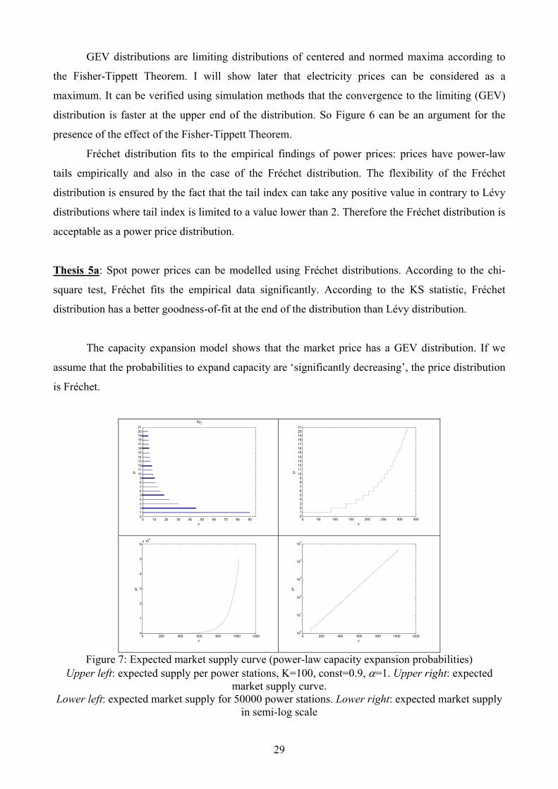
The capacity expansion model shows that the market price has a GEV distribution. If we

assume that the probabilities to expand capacity are ‘significantly decreasing’, the price distribution

is Fréchet.

0 10 20 30 40 50 60 70 80 900123456789

101112131415161718192021

x

pr

Kpi

0 50 100 150 200 250 300 350

0123456789

101112131415161718192021

x

pr

0 200 400 600 800 1000 12000

1

2

3

4

5

6x 104

x

pr

0 200 400 600 800 1000 1200

100

101

102

103

104

105

x

pr

Figure 7: Expected market supply curve (power-law capacity expansion probabilities)

Upper left: expected supply per power stations, K=100, const=0.9, α=1. Upper right: expected market supply curve.

Lower left: expected market supply for 50000 power stations. Lower right: expected market supply in semi-log scale

30

How realistic is the assumption that probabilities of capacity expansion are ‘significantly

decreasing’? To answer this question we have to analyze power supply. Given the pi capacity

expansion probability for power station i and the K size of demand, then the expected supply of

power station i is xi = Kpi. Construct an expected market supply curve from these expected supplies,

and then we will see that the price is an exponential function of the quantity if the pi probabilities

are decaying according to the power-law like 0.9/i (see Figure 7). So in our model the market price

has a Fréchet distribution if the market supply curve shows that the price is an exponential function

of the quantity. In reality, day-ahead electricity market supply curves are found to be exponential

(Bunn [2004]). We can conclude that the ‘significantly decreasing’ behaviour of capacity expansion

probabilities and the Fréchet distribution are in connection with the exponential markets supply

curve. Of course, market supply curve is not perfectly exponential, but any market supply curve

close to exponential will imply power-law winning probabilities and ‘significantly decreasing’

capacity expansion probabilities, because (as we have seen) slight modifications in the market

supply curve and therefore in the capacity expansion probabilities implied by Figure 7 still give

‘strongly decreasing’ expansion probabilities and Fréchet distribution.

Thesis 5b: I built a capacity expansion model which I used to demonstrate that the presence of the

Fréchet distribution in electricity markets is caused by the exponential market supply curve.

Extreme value theory and specifically the Fisher-Tippett Theorem were used to get to this

conclusion. The key assumptions of the model were that electricity demand is fixed and demand

units are auctioned separately.

Hypothesis 6

(Electricity prices can be described using a regime switching model where prices change

regimes deterministically.)

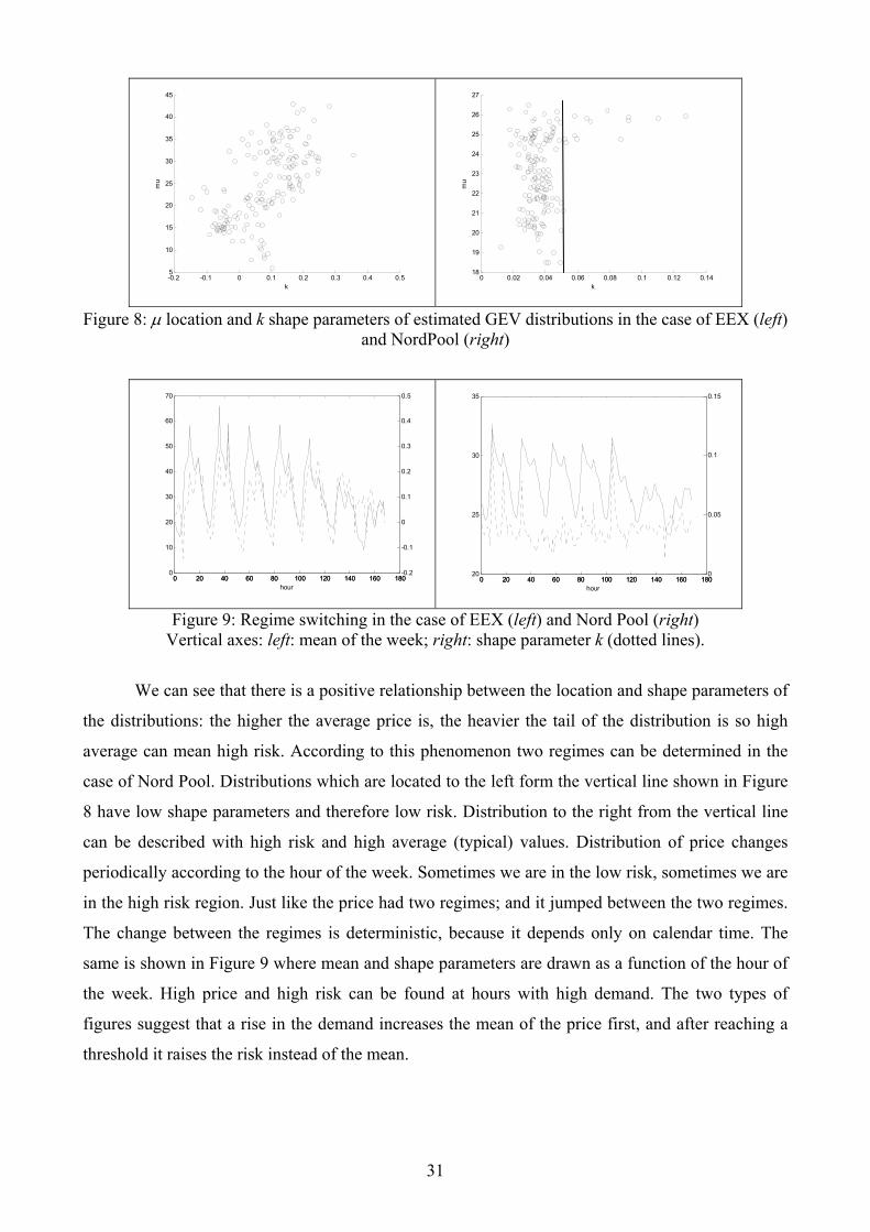
168 GEV distributions were fitted to the segments. The connection of the location and shape

parameters is visualized in Figure 8.

31

-0.2 -0.1 0 0.1 0.2 0.3 0.4 0.55

10

15

20

25

30

35

40

45

k

mu

0 0.02 0.04 0.06 0.08 0.1 0.12 0.1418

19

20

21

22

23

24

25

26

27

k

mu

Figure 8: µ location and k shape parameters of estimated GEV distributions in the case of EEX (left) and NordPool (right)

0 20 40 60 80 100 120 140 160 1800

10

20

30

40

50

60

70

0 20 40 60 80 100 120 140 160 180-0.2

-0.1

0

0.1

0.2

0.3

0.4

0.5

hour0 20 40 60 80 100 120 140 160 180

20

25

30

35

0 20 40 60 80 100 120 140 160 1800

0.05

0.1

0.15

hour

Figure 9: Regime switching in the case of EEX (left) and Nord Pool (right) Vertical axes: left: mean of the week; right: shape parameter k (dotted lines).

We can see that there is a positive relationship between the location and shape parameters of

the distributions: the higher the average price is, the heavier the tail of the distribution is so high

average can mean high risk. According to this phenomenon two regimes can be determined in the

case of Nord Pool. Distributions which are located to the left form the vertical line shown in Figure

8 have low shape parameters and therefore low risk. Distribution to the right from the vertical line

can be described with high risk and high average (typical) values. Distribution of price changes

periodically according to the hour of the week. Sometimes we are in the low risk, sometimes we are

in the high risk region. Just like the price had two regimes; and it jumped between the two regimes.

The change between the regimes is deterministic, because it depends only on calendar time. The

same is shown in Figure 9 where mean and shape parameters are drawn as a function of the hour of

the week. High price and high risk can be found at hours with high demand. The two types of

figures suggest that a rise in the demand increases the mean of the price first, and after reaching a

threshold it raises the risk instead of the mean.

32

Thesis 6: Hours of the week have different price distributions. Some hours with high mean have

heavier tail and increased price risk. As distributions are changing periodically according to the

hour of the week, I named this phenomenon ‘deterministic regime switching’.

Hypothesis 7

(Seasonality can be removed by changing the type of distributions.)

The performance of the GEV filter is illustrated with the periodogram of original and filtered

data in Figure 10. It can be seen that spikes indicating intra-weekly seasonality disappeared from

the periodogram so filtering the intra-weekly seasonality was successful. Spikes belonging to 168

hours and its multiples are still present after the filtering. These spikes indicate seasonality beyond a

week so there was no intention to remove them.

0 0.1 0.2 0.3 0.4 0.5 0.6 0.7 0.8 0.9 1-70

-60

-50

-40

-30

-20

-10

0

10

20

30

Normalized Frequency (×π rad/sample)

Pow

er/fr

eque

ncy

(dB

/rad/

sam

ple)

Power Spectral Density Estimate via Periodogram

0 0.1 0.2 0.3 0.4 0.5 0.6 0.7 0.8 0.9 1-70

-60

-50

-40

-30

-20

-10

0

10

20

Normalized Frequency (×π rad/sample)

Pow

er/fr

eque

ncy

(dB

/rad/

sam

ple)

Power Spectral Density Estimate via Periodogram

Figure 10: Periodogram of NordPool prices before (left) and after (right) filtering

Thesis 7a: Intra-weekly seasonality can be removed by changing the type of the distribution: a

transformation is defined using the cdf of lognormal and GEV distributions. (GEV-filter)

As the GEV filter transforms the Fréchet distribution with heavy tails into a lognormal

distribution with exponential tails, the effect of fat tails is dissolved by the filtering procedure. As

the different distributions are transformed to the same (lognormal) distribution, the deterministic

regime switching phenomenon caused by the diverse distributions disappears. Moreover, the GEV

filter removes the effect of price spikes and seasonality at the same time, so it resolves the problem

of the interconnection of the two filtering procedures.

Thesis 7b: GEV filter removes price spikes and deterministic regime switching.

33

I investigated the effect of GEV filtering on the Hurst exponent of the time series. Table 4

has the estimation results in the case of EEX and Nord Pool. Thesis 7c concludes.

EEX Nord Pool Price Filtered price Price Filtered price

R/S 0.88 (0.0929)

0.78 (0.0350)

0.87 (0.0399)

0.93 (0.0465)

Aggregated Variance 0.86 (0.0167)

0.86 (0.0258)

0.99 (0.0244)

0.99 (0.0365)

Differenced Variance 0.79 (0.0505)

0.85 (0.1341)

0.98 (0.2064)

1.02 (0.1902)

Periodogram regression 0.83 (0.0037)

0.89 (0.0079)

1.21 (0.0037)

1.08 (0,0062)

AWC 0.85 (0.0874)

0.93 (0,0587)

0.93 (0,0480)

0.98 (0,0601)

h(2) 0.84 0.90 1.15 1.18 hmod(2) 0.83 0.90 1.14 1.19

Table 4: Estimated Hurst exponents for the original and filtered prices Standard errors are shown in parenthesis.

Thesis 7c: The GEV filtering procedure will not change the estimated value of the Hurst exponent

significantly.

It is not straightforward to determine the behaviour of the GEV-filtered prices. The GEV

filtering procedure is a complex transformation which ruins the structure of linear correlations.

Although it is not trivial to derive the connection between the behaviour of the original and the

filtered prices, we can find connections between the two systems. We have seen in Thesis 7c that

the long-term correlation structure will not change during the GEV filtering procedure, therefore the

GEV-filtered prices can be modelled by using basically the models as the original prices.

Fortunately, the complexity of the time series (e.g. spikes, seasonality) was simplified by using the

GEV filter.

Besides the autocorrelations, another question arises in the framework of the deterministic

regime switching model and the GEV filter. They assume that the price distribution is different for

each hour, but it is the same in the case of the same hour across weeks. It is apparently not true

because e.g. we have a trend in the prices. Therefore, it is suggested to remove the trends from the

data. During the empirical analysis of Hypothesis 7, I removed an exponential trend form the time

series before the filtering. The modeller has to consider which trends to remove from the time series

(e.g. systematic changes in the power generation input prices). The GEV filter can be applied after

we have removed the trend component.

34

During the power price modelling procedure, we have to remove the trend (and the cyclical

component) from the data, and then we should transform the data using the GEV filter. Finally we

have to find a proper model on the resulting time series. My proposed modelling framework is the

following:

( )EfCTY S++=

where Y stands for the power price, T is the trend, C is the cyclical component, S denotes the

seasonality effect, and E denotes the error (random) term.

Empirical model

The results of my thesis were used by Ujfalusi [2008]. She succeeded to fit a significant

ARMA-GARCH model on the GEV filtered and long memory filtered price. According to this, long

memory filtering and GEV filtering can be effectively used during the modelling process. The

effects which are not filtered using these two preprocessing methods can be easily modelled using

autoregressive and GARCH terms. Without these two filtering procedure the model for the power

price would have been more complex, more difficult, and not transparent enough.

35

Conclusions

In the light of the results we can reconsider the stylized facts of power prices. Numbers in

brackets refer to the numbers of the theses.

1. There are high prices (price spikes) in the time series.

Extremely high electricity prices are inherent in the price series. These ‘price spikes’ are not

outliers appearing out of the blue, but they are high realizations from a fat-tailed random variable

describing the power price (4). The probability of high prices is higher in some periods, but the

reason of the higher risk of high prices is the fact that we are in a riskier hour of the week so the risk

is deterministic (6). Of course we cannot state that we will have a price spike in this hour, but we

can say indeed that the probability of occurrence is higher. The theories explaining price spikes with

supply and demand shocks are not questioned here as the reason of changing GEV parameters lies

in the structure of supply and demand.

2. High autocorrelation.

According to the results of the thesis, one of the reasons of the slowly decaying autocorrelation

function is the long memory of the process (1a). The periodicity of the autocorrelation function is

caused by the seasonality which can be removed using the GEV filter (7).

3. The volatility is changing in time, the time series is heteroskedastic.

Heteroskedasticity is partly caused by the fact that distributions of power prices belonging to

different hour of the week are not the same as they stem from GEV distributions with different

parameters (6). Periodically changing GEV distributions do not explain the heteroskedasticity

feature completely: as we have seen in the empirical model, one can fit a significant GARCH model

even after applying the GEV filter.

4. The time series exhibits seasonality.

Seasonality is caused by the periodically changing GEV distributions (6). GEV distributions

also describe the seasonal feature of volatility. Seasonality caused by the periodically changing

distributions can be filtered if we transform the distributions into a common distribution (7). My

GEV filter transforms the data into the lognormal distribution.

36

5. Price and log-return distributions have fat tails.

Power prices have GEV, namely Fréchet distribution (5a). Fat tails are incorporated by the

power-law tail of the Fréchet distribution. In a capacity expansion model I showed that the Fréchet

distribution and fat tails have the reason that price is an exponential function of the quantity in the

market supply curve (5b). To put it differently: fat tails are caused by the fact that power stations

with low marginal cost can expand their capacity with a higher probability on the average.

6. Some authors argue that power prices are anti-persistent and mean reverting; meanwhile

others state that the price time series has long memory. According to researches, electricity

has a multifractal price process.

My analysis shows that power prices are persistent with a Hurst exponent between 0.8 and 1

(1a). The diverse results in the literature stem from the fact that papers are analyzing different

underlying variables (1a). We can reproduce the persistency results of some papers if we analyze

the log-return instead of the price. In my opinion, it is not useful to deal with the Hurst exponent of

the log-return though as the log-return process does not have clear self affine property (1b).

Therefore it does not make sense to use log-return instead of the price for modelling purposes if we

have no other reason to do so (2).

7. There is no consensus whether the price process has a unit root indicating the integratedness

of the process.

I do not deal with formal unit root tests in my thesis. My result analyzing the Hurst exponent (1)

convinced me however that it is useful to use the price instead of the log-return for modelling

purposes as the price process has better mathematical features, log-return can not be interpreted

directly, and we have no statistical pressure to use the log-price: there is no clear evidence that the

price process has a unit root (2).

As the main result of the thesis, I showed that the trading procedure results in a common

(GEV) price distribution for each hour in the day-ahead power market. Price spikes are present as

the fat tails of these distributions. Due to the periodicity of power demand (and supply), the

distributions are changing periodically. We can use this phenomenon to remove the seasonality

form the time series. Price spikes (fat tails) and part of the heteroscedasticity is also removed during

the seasonality filtering (by changing the hourly distributions).

In my power price model, the (persistent) random terms are transformed by a seasonality

effect which changes the distribution of hourly prices, and then a trend and a cyclical component is

37

added. The modelling procedure will not become more difficult as in the case of additive

seasonality. We can model the filtered random term more easily by using my modelling framework.

Empirical application of the results is possible in the following areas:

Hurst exponents can be used without any further misunderstanding so the model choice has

been supported (long memory, monofractal feature).

I drew attention to the inappropriate statistical features of the log-price so that modellers are

reminded to use it more carefully during the modelling procedure.

Price spikes can be modelled using fat-tailed distributions and not with a separate regime.

Medium and long term price forecasts are supported by providing the conditional (time-

dependent) distribution of power prices.

I helped short term price forecast by designing a seasonality filter.

Conditional price distribution can be analyzed using the market supply curve.

The deterministic regime switching model with periodically changing GEV parameters can

be used to model price spikes, seasonality and changing parameters.

My future research plan has many directions in accordance with the presented models, e.g.

developing a theoretical background for a high risk early warning system;

fitting an ARFIMA-GARCH model on GEV-filtered power prices and evaluate the quality

of price forecasting;

exploring the relationship of the estimated GEV parameters in the deterministic regime

switching model (e.g. relationship of the scale and shape parameter);

comparing the GEV filter with other filtering methods using empirical data and forecasting.

38

Selected bibliography

De Jong, Cyriel [2006]: The Nature of Power Spikes: A Regime-Switch Approach. Studies in

Nonlinear Dynamics & Econometrics. Vol 10 (3).

Embrechts, Paul – Klüppelberg, Claudia – Mikosch, Thomas [2003]: Modelling Extremal Events

for Insurance and Finance. Corrected Fourth Printing. Springer. Heidelberg, Germany.

Erzgräber, Hartmut – Strozzi, Fernanda – Zaldívar, José-Manuel – Touchette, Hugo – Gutiérrez,

Eugénio – Arrowsmith, David K. [2008]: Time series analysis and long range correlations

of Nordic spot electricity market data. Physica A. Vol 387 (26), pp. 6567-6574.

Eydeland, Alexander – Wolyniec, Krzysztof [2003]: Energy and Power Risk Management. New

Developments in Modeling, Pricing, and Hedging. John Wiley & Sons, Hoboken, New

Jersey, U.S.A.

Geman, Hélyette – Roncoroni, Andrea [2006]: Understanding the Fine Structure of Electricity

Prices. Journal of Business. Vol 79 (3), pp. 1225-1261.

Haldrup, Niels – Nielsen, Morten Ørregaard [2006]: A regime switching long memory model for

electricity prices. Journal of Econometrics. Vol 135, pp. 349-376.

Jiang, Zhi-Qiang – Zhou, Wei-Xing [2007]: Multifractality in stock indexes: Fact or fiction?

Physica A. Vol 387, pp. 3605-3614.

Kantelhardt, Jan W. – Zschienger, Stephan A. – Koscielny-Bunde, Eva – Havlin, Shlomo – Bunde,

Armin – Stanley, H. Eugene [2002]: Multifractal detrended fluctuation analysis of

nonstacionary time series. Physica A. Vol 316, pp. 87-114.

McNeil, Alexander J. – Frey, Rüdiger – Embrechts, Paul [2005]: Quantitative Risk Management.

Concepts, Techniques and Tools. Princeton University Press. Princeton Series in Finance.

Princeton, U.S.A.

Misiorek, A. – Trück, S. – Weron, R. [2006]: Point and Interval Forecasting of Spot Electricity

Prices: Linear vs Non-Linear Time Series Models. Studies in Nonlinear Dynamics and

Econometrics. Vol 10 (3), Article 2.

Montanari, Alberto – Rosso, Renzo – Taqqu, Murad S. [1997]: Fractionally differenced ARIMA

models applied to hydrologic time series: Identification, estimation, and simulation. Water

Resources Research. Vol 33 (5), pp. 1035-1044.

Norouzzadeh, P. – Dullaert, W. – Rahmani, B. [2007]: Anti-correlation and multifractal features of

Spain electricity spot market. Physica A. Vol 380, pp. 333-342.

Serletis, Apostolos – Andreadis, Ioannis [2004]: Nonlinear Time Series Analysis of Alberta’s

Deregulated Electricity Market. In: Bunn, Derew W. (ed.): Modelling prices in competitive

electricity markets. John Wiley & Sons. Wiley Finance Series. Chichester, England.

39

Simonsen, Ingve [2003]: Measuring Anti-Correlations int he Nordic Electricity Spot Market by

Wavelets. Physica A. Vol 322, pp. 597-606.

Simonsen, Ingve – Weron, Rafal – Mo, Birger [2004]: Structure and stylized facts of a deregulated

power market. Working paper. 1st Bonzenfreies Colloquium on Market Dynamics and

Quantitative Economics.

Trück, Stefan – Weron, Rafal – Wolff, Rodney [2007]: Outlier Treatment and Robust Approaches

for Modeling Electricity Spot Prices. Working paper. Munich Personal RePEc Archive

4711.

Ujfalusi Dóra [2008]: Kockáztatott érték és extrémérték-elmélet a villamosenergia-piacon. Master’s

thesis. Budapesti Corvinus Egyetem.

Weron, Rafal [2000]: Energy price risk management. Physica A. Vol 285, pp. 127-134.

Weron, Rafal [2006]: Modeling and forecasting electricity loads and prices. A Statistical Approach.

John Wiley & Sons. Wiley Finance Series. Chicsester, England.

Weron, Rafal [2008a]: Heavy-tails and regime-switching in electricity prices. Mathematical

Methods of Operations Research. Forthcoming.

Weron, Rafal [2008b]: Market price of risk implied by Asian-style electricity options. Energy

Economics. Vol 30 (3), pp. 1098-1115.

Weron, Rafal – Przybyłowitz, Beata [2000]: Hurst analysis of electricity price dynamics. Physica A.

Vol 283, pp. 462-468.

Please find the full list of literature in the thesis.

40

Own publications in the research field of the thesis

(Alternate names: Zita Marossy, Zita Petrimán)

Marossy Zita [2010]: Multifractality testing of Markov regime switching models in spot electricity

price modelling. Proceedings of ‘Spring wind’ Conference 2010, pp. 315-320.

Marossy Zita [2010]: Hurst exponent of deseasonalized spot electricity prices. Proceedings of

XXIV. microCAD International Scientific Conference, Section: Energy Management, pp.

27-32.

Marossy Zita [2009]: The behaviour of day-ahead electricity prices. MANMADE Workshop on

Deregulated European Energy Market. Budapest, September 24-25, 2009.

Marossy Zita [2008]: A spot villamosenergia-árak szezonális szűrése. Proceedings of ‘Tavaszi Szél’

Conference 2008, pp. 211-219.

Marossy Zita [2008]: Seasonality filtering of spot electricity prices using GEV distributions.

Computers and Algorithms in Mathematical Economics and Finance Conference. Budapest,

January 29 – February 1, 2008.

Marossy Zita – Szenes Márk [2008]: Analysis of day-ahead electricity data. MANMADE

workshop. Budapest, January 21-22, 2008.

Marossy Zita [2007]: A villamosenergia-árak modellezése extrémérték-elmélet alapján. 3rd Annual

Conference of the PhD School of Economics. Budapest, December 14, 2007.

Marossy Zita [2007]: Modeling electricity prices using extreme value theory. Inter-departmental

conference. Organizer: BCE Department of Finance and Universität Passau Lehrstuhl für

Finanzierung. Budapest, December 7, 2007.

Marossy Zita [2007]: EVT in electricity price modeling: extreme value theory not only on the

extreme events. Proceedings of EuroPES 2007 Conference. Palma de Mallorca, pp. 319-

323.

Marossy Zita [2007]: A villamosenergia-árak modellezése. Proceedings of ‘Tavaszi Szél’

Conference 2007, social sciences, pp. 336-341.

Marossy Zita [2006]: Villamosenergia-piacok modellezése. 2nd Annual Conference of the PhD

School of Economics. Budapest, November 24, 2006.

Petrimán Zita [2005]: A villamosenergia-árak modellezése: itt az idősor, hol az idősor. Proceedings

of ‘Tavaszi Szél’ Conference 2005, pp. 324-327.

Petrimán Zita – Tulassay Zsolt [2005]: Bepillantás az ARCH modellek világába. Hitelintézeti

Szemle (4) Vol 2, pp. 74-79.