Peter Fortune

Professor of Economics at Tufts Uni-versity. The author did the basic re-search for this article while he was aVisiting Scholar at the Federal ReserveBank of Boston in 1990-91. He isgrateful to the Federal Reserve Bank ofBoston for research support.

Fifty years ago Henry C. Simons challenged the concept of taxexemption when he remarked (1938):

The exemption of the interest payments on an enormous amount of govern-ment bonds.., is a flaw of major importance. It opens the way to deliberateavoidance on a grand scale ... the exemption not only undermines theprogram of progressive personal taxation but also introduces a large measureof differentiation in favor of those whose role in our economy is merely thatof rentiers.

While the "program of progressive personal taxation" appears tohave been left behind, Simons’ criticism of the exemption is still widelyheld. The purpose of this article is to identify the problems posed by taxexemption, and to assess some alternatives. The analysis goes wellbeyond the issue of equity, which is the heart of Simons’ complaint. Thisstudy asks whether the results of tax exemption represent an appropri-ate outcome, and questions whether tax exemption is really necessary toachieve the benefits stated in its favor.

This article is a companion to an earlier one (Fortune 1991) thatexamined the effects of the income tax code on the market for municipalbonds, concluding that the municipal bond market is a creature of taxpolicy. That article explored the history of the exemption, reviewed therelevant tax legislation, presented a theoretical model of the municipalbond market, and employed econometric methods to determine the roleplayed by the tax code.

The first section of this article addresses three major problems ofmunicipal bond market performance: market instability, vertical equity,and financial efficiency. These problems have driven the debate aboutreform of the market. The second section discusses several approachesto mitigating these problems. The third section focuses on an aspect oftax exemption that has received very little attention, its impact on

resource allocation and economic efficiency. The sec-tion estimates the loss in economic output due to theexemption, concluding that while the loss is smallrelative to the size of the economy, it is, nevertheless,worthy of attention. The last section summarizes thearticle and its conclusions.

L Municipal Bond Market PerformanceWhy does Congress allow municipal interest

payments to be exempted from federal income taxesin the face of a very large chronic deficit in the federalbudget, even though it is now clear that no constitu-tional provision requires that this tax policy continue?The rhetoric of tax exemption is philosophical, ap-pealing to notions of appropriate intergovernmentalrelations and, in particular, to the doctrine of recip-rocal immunity: no level of government should useits taxing authority to impose harm on another level.But the true force behind tax exemption is that itprovides state and local governments with a valuablesubsidy, which can be enjoyed at their discretion.Political support for the exemption is very strong,and it will continue unless a better way can be foundto structure a subsidy to state and local governments.

An assessment of the economics of tax exemp-tion, which is a subsidy of capital costs, suggests thatthe case for it is weak. The economic argument must

The true force behind taxexemption is that it providesstate and local governments

with a valuable subsidy,which can be enjoyed at

their discretion.

rest on the view that, in the absence of a capital costsubsidy, state and local governments will produce aninadequate amount of public services with insuffi-cient capital intensity. While the final word on thisissue is not yet spoken, the debate continues in thecurrent discussion about public infrastructure, suchas highways, schools, and solid waste facilities. For

example, Munnell (1990) finds a high marginal pro-ductivity of infrastructure, suggesting that an inade-quate amount is available, while Hulten and Schwab(1991) find no indication of inadequate infrastructure.

However, even if infrastructure is insufficient, itcan be argued that better methods than tax exemp-tion can be used to achieve these goals. Three funda-mental criticisms of tax exemption have received themost attention. The first says that tax exemptioninduces unnecessary volatility into municipal bondyields. According to this "market instability" argu-ment, tax exemption narrows the market for munic-ipal bonds and makes that market more sensitive tochanges in the distribution of investable funds be-tween individuals and financial institutions, as wellas to other factors that affect financial markets. Theresult is that municipal bond yields are more volatilethan yields on comparable taxable bonds, introducingcyclical variations in the cost of capital for state andlocal governments. This also introduces variabilityinto the value of the capital-cost subsidy enjoyed bymunicipalities.

The second criticism, echoing Simons’ com-plaint, is that tax exemption is inequitable; it confersupon the wealthy a valuable opportunity to increasetheir after-tax income, and it erodes the degree ofvertical equity in our tax system by allowing thewealthy to avoid taxation in ways not available to theless affluent. This criticism is the most common inpopular discussions of tax exemption.

The third criticism is that tax exemption isfinancially inefficient because it imposes greater costson federal taxpayers than the benefits it confers uponstate and local governments. 1 Still another criticism isthat tax exemption fails to encourage economicefficiency. Instead, it is argued, tax exemption en-courages overproduction of public services as well asoveruse of capital by the public sector. A corollary isthat the private sector has inadequate capital withwhich to produce goods and services. This view isbased on the assumption that a competitive marketeconomy, unfettered by government intervention inprices, will induce an appropriate allocation of re-sources. This issue will be discussed in the thirdsection of the article.

1 Note that the word "efficiency" in this context is used quitedifferently from the engineering context (getting the most for anygiven amount of inputs) or the economic context (Pareto-Optimal-ity, or making each person as well off as possible given thepositions of all other people). The focus of financial efficiency is onthe very narrow question of how much benefit is received by lowerlevels of government per dollar of cost to the federal Treasury.

48 May/June 1992 New England Economic Review

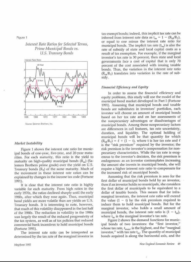
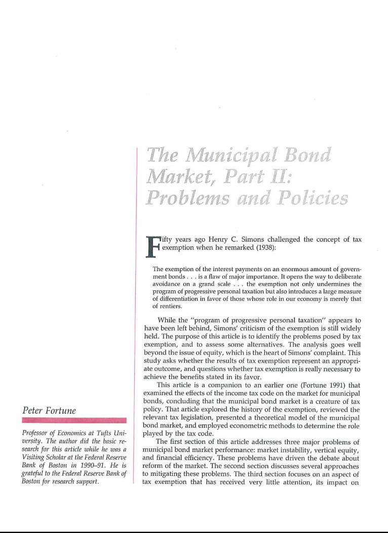
Figure 1

Interest Rate Ratios for Selected Terms,Prime Municipal Bonds vs.

U.S. Treasury Bonds

Interest Rate Ratio

20-Year

1-Year4

1965 i969 1973 1977 1981 1985 1989

Source: Satomon Brothers, Inc.

Market Instability

Figure 1 shows the interest rate ratio for munic-ipal bonds of one-year, five-year, and 20-year matu-rities. For each maturity, this ratio is the yield tomaturity on high-quality municipal bonds (Rm) (Sa-lomon Brothers prime grade) over the yield on U.S.Treasury bonds (RT) of the same maturity. Much ofthe movement in these interest rate ratios can beexplained by changes in the income tax code (Fortune1991).

It is clear that the interest rate ratio is highlyvariable for each maturity. From high ratios in theearly 1970s, the ratios declined sharply until the early1980s, after which they rose again. Thus, municipalbond yields are more volatile than are yields on U.S.Treasury bonds. It is interesting to note, however,that much of this volatility disappeared in the last halfof the 1980s. The reduction in volatility in the 1980swas largely the result of the reduced progressivity ofthe tax system, as well as of tax policies that reducedcommercial bank incentives to hold municipal bonds(Fortune 1991).

The interest rate ratio can be interpreted asdetermined by the tax rate of the marginal investor in

tax-exempt bonds; indeed, this implicit tax rate can beinferred from interest rate data as trn = 1 - (RM/RT),or equal to one minus the interest rate ratio formunicipal bonds. The implicit tax rate (tin) is also therate of subsidy of state and local capital costs as aresult of tax exemption. For example, if the marginalinvestor’s tax rate is 30 percent, then state and localgovernments face a cost of capital that is only 70percent of the cost associated with issuing taxablebonds. Thus, the variation in the interest rate ratio(Rn~/RT) translates into variation in the rate of sub-sidy.

Financial Efficfency and Equfty

In order to assess the financial efficiency andequity problems, this study will use the model of themunicipal bond market developed in Part I (Fortune1991). Assuming that municipal bonds and taxablebonds are substitutes in investors’ portfolios, eachinvestor will choose an amount of municipal bondsbased on her tax rate and on her assessments ofthe nonpecuniary advantages or disadvantages ofmunicipal bonds. Among these nonpecuniary factorsare differences in call features, tax rate uncertainty,duration, and liquidity. The optimal holding ofmunicipal bonds will be that quantity for which(RM/RT) = ~ + (1 -- t), where t is her tax rate and ~7is the "risk premium" required by the investor; therisk premium is the investor’s compensation for non-pecuniary characteristics. While the tax rate is exog-enous to the investor’s decision, the risk premium isendogenous: as an investor contemplates increasingthe amount she invests in municipal bonds, she willrequire a higher interest rate ratio to compensate forthe increased risk of municipal bonds.

Assuming that the risk premium is zero for thefirst dollar of municipal bonds held by an investor,then if an investor holds no municipals, she considersthe first dollar of municipals to be equivalent to adollar of taxable bonds. This means that for infra-marginal investors, the interest rate ratio will exceedthe value (1 - t) by the risk premium required toinduce them to hold municipal bonds. But for themarginal investor, who holds a small amount ofmunicipal bonds, the interest rate ratio is (1 - t~),where t~ is the marginal investor’s tax rate.

Figure 2 shows the demand functions for munic-ipal bonds of two investors: the "first investor,"whose tax rate, tmax, is the highest, and the "marginalinvestor," with tax rate t~. The quantity of municipalbonds acquired is along the horizontal axis, and the

MaylJune 1992 Nezo Englamt Economic Review 49

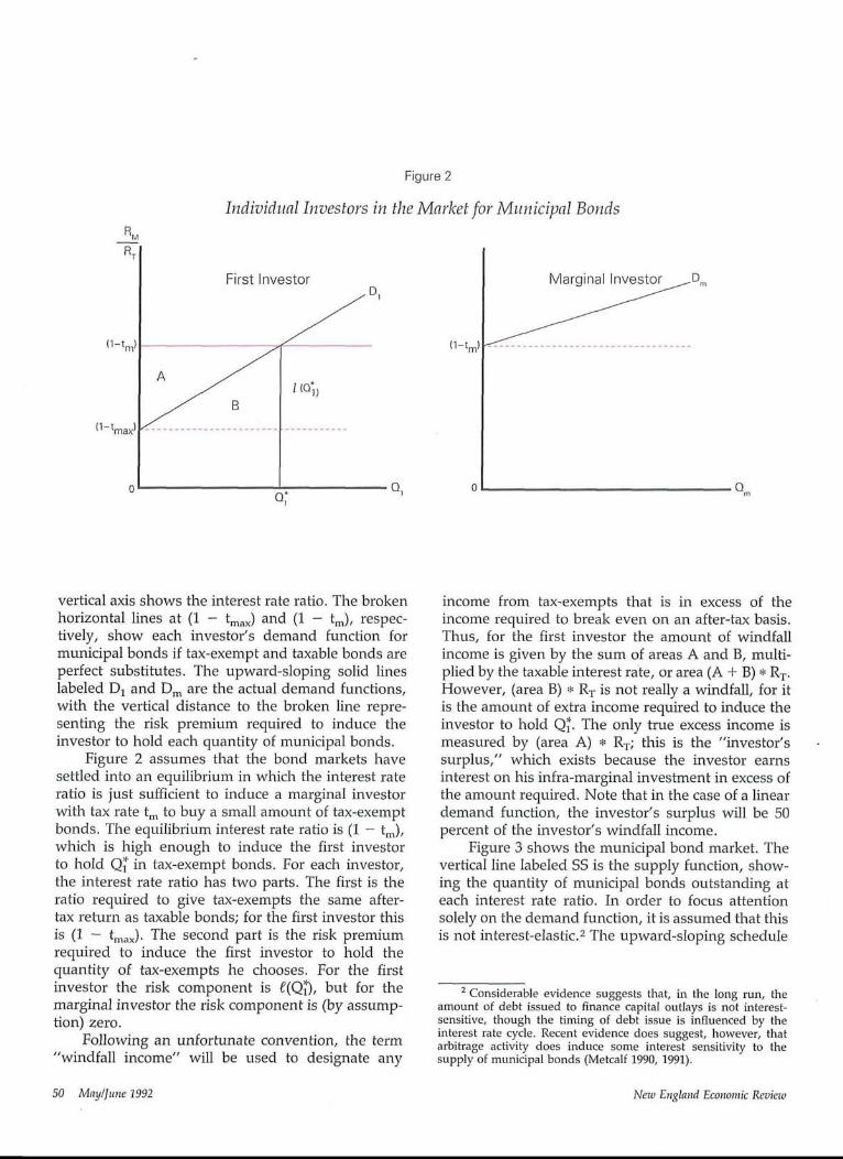
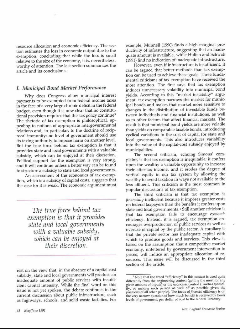
Figure 2

Individual h~vestors in the Market for Municipal Bonds

First Investor Marginal InvestorD1

I (01)

(1-tmax)

Qm

vertical axis shows the interest rate ratio. The brokenhorizontal lines at (1 - tmax) and (1 - tin), respec-tively, show each investor’s demand function formunicipal bonds if tax-exempt and taxable bonds areperfect substitutes. The upward-sloping solid lineslabeled D1 and Dm are the actual demand functions,with the vertical distance to the broken line repre-senting the risk premium required to induce theinvestor to hold each quantity of municipal bonds.

Figure 2 assumes that the bond markets havesettled into an equilibrium in which the interest rateratio is just sufficient to induce a marginal investorwith tax rate tm to buy a small amount of tax-exemptbonds. The equilibrium interest rate ratio is (1 - tm),which is high enough to induce the first investorto hold Q~ in tax-exempt bonds. For each investor,the interest rate ratio has two parts. The first is theratio required to give tax-exempts the same after-tax return as taxable bonds; for the first investor thisis (l -- tmax). The second part is the risk premiumrequired to induce the first investor to hold thequantity of tax-exempts he chooses. For the firstinvestor the risk component is e(Q~, but for themarginal investor the risk component is (by assump-tion) zero.

Following an unfortunate convention, the term"windfall income" will be used to designate any

income from tax-exempts that is in excess of theincome required to break even on an after-tax basis.Thus, for the first investor the amount of windfallincome is given by the sum of areas A and B, multi-plied by the taxable interest rate, or area (A + B) * RT.However, (area B) * RT is not really a windfall, for itis the amount of extra income required to induce theinvestor to hold Q~. The only true excess income ismeasured by (area A) * RT; this is the "investor’ssurplus," which exists because the investor earnsinterest on his infra-marginal investment in excess ofthe amount required. Note that in the case of a lineardemand function, the investor’s surplus will be 50percent of the investor’s windfall income.

Figure 3 shows the municipal bond market. Thevertical line labeled SS is the supply function, show-ing the quantity of municipal bonds outstanding ateach interest rate ratio. In order to focus attentionsolely on the demand function, it is assumed that thisis not interest-elastic.2 The upward-sloping schedule

2 Considerable evidence suggests that, in the long run, theamount of debt issued to finance capital outlays is not interest-sensitive, though the timing of debt issue is influenced by theinterest rate cycle. Recent evidence does suggest, however, thatarbitrage activity does induce some interest sensitivity to thesupply of municipal bonds (Metcalf 1990, 1991).

50 May/June 1992 New England Economic Reviezo

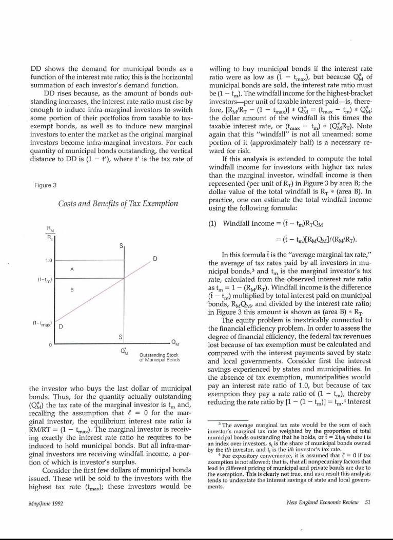
DD shows the demand for municipal bonds as afunction of the interest rate ratio; this is the horizontalsummation of each investor’s demand function.

DD rises because, as the amount of bonds out-standing increases, the interest rate ratio must rise byenough to induce infra-marginal investors to switchsome portion of their portfolios from taxable to tax-exempt bonds, as well as to induce new marginalinvestors to enter the market as the original marginalinvestors become infra-marginal investors. For eachquantity of municipal bonds outstanding, the verticaldistance to DD is (1 - t’), where t’ is the tax rate of

Figure 3

Costs and Benefits of Tax Exemption

RM

1.0

(1-tm)

(1-tmax)

B

D

QM

Outstanding Stockof Municipal Bonds

the investor who buys the last dollar of municipalbonds. Thus, for the quantity actually outstanding(Q~) the tax rate of the marginal investor is tm and,recalling the assumption that ~ = 0 for the mar-ginal investor, the equilibrium interest rate ratio isRM!RT = (1 - tma×). The marginal investor is receiv-ing exactly the interest rate ratio he requires to beinduced to hold municipal bonds. But all infra-mar-ginal investors are receiving windfall income, a por-tion of which is investor’s surplus.

Consider the first few dollars of municipal bondsissued. These will be sold to the investors with thehighest tax rate (tma×); these investors would be

willing to buy municipal bonds if the interest rateratio were as low as (1 - tma×), but because Q~ ofmunicipal bonds are sold, the interest rate ratio mustbe (1 - tm). The windfall income for the highest-bracketinvestors--per unit of taxable interest paid is, there-fore, [RM/Rw - (1 - tmax)] * Q~ = (trnax -- tm) * Q~;the dollar amount of the windfall is this times thetaxable interest rate, or (trnax -- tm) * (Q~RT). Noteagain that this "windfall" is not all unearned: someportion of it (approximately halO is a necessary re-ward for risk.

If this analysis is extended to compute the totalwindfall income for investors with higher tax ratesthan the marginal investor, windfall income is thenrepresented (per unit of RT) in Figure 3 by area B; thedollar value of the total windfall is RT * (area B). Inpractice, one can estimate the total windfall incomeusing the following formula:

(1) Windfall Income = (~ - tm)RTQM

= (~ -- tm)[RMQM]/(RM/RT).

In this formula [ is the "average marginal tax rate,"the average of tax rates paid by all investors in mu-nicipal bonds,3 and tm is the marginal investor’s taxrate, calculated from the observed interest rate ratioas tm = 1 - (RM/RT). Windfall income is the difference(~ - tm) multiplied by total interest paid on municipalbonds, RMQM, and divided by the interest rate ratio;in Figure 3 this amount is shown as (area B) * RT.

The equity problem is inextricably connected tothe financial efficiency problem. In order to assess thedegree of financial efficiency, the federal tax revenueslost because of tax exemption must be calculated andcompared with the interest payments saved by stateand local governments. Consider first the interestsavings experienced by states and municipalities. Inthe absence of tax exemption, municipalities wouldpay an interest rate ratio of 1.0, but because of taxexemption they pay a rate ratio of (1 - tm), therebyreducing the rate ratio by [1 - (1 - tin)] = tm.4 Interest

3 The average marginal tax rate would be the sum of eachinvestor’s marginal tax rate weighted by the L~roportion of totalmunicipal bonds outstanding that he holds, or t = ~tisi where i isan index over investors, si is the share of municipal bonds ownedby the ith investor, and t~ is the ith investor’s tax rate.

4 For expository convenience, it is assumed that f = 0 if taxexemption is not allowed; that is, that all nonpecuniary factors thatlead to different pricing of municipal and private bonds are due tothe exemption. This is clearly not true, and as a result this analysistends to understate the interest savings of state and local govern-ments.

May/June 1992 Nezv England Economic Review 51

savings is, therefore, measured by (area A) * RT,which is

(2) Interest Savings = tmRTQM.

The revenue cost to the U.S. Treasury is the sumof two components: the windfall income received byhigh-bracket investors plus the interest savings ofmunicipalities. The dollar value of revenue cost is(area A + area B) * RT. Thus,

(3) Revenue Cost = RT * [tm + (~ - tm)]QM

= ~RTQM.

If, as has historically been true in the United States,taxation of income is progressive, then the average mar-ginal tax rate exceeds the marginal tax rate (t > tm)and area (A + B) > area A. Therefore the revenuecost to the federal government must exceed theinterest savings enjoyed by states and local govern-ments by an amount known as "windfall income."

Thus, the financial inefficiency of tax exemptionexists because of the equity problem, and reductionof the equity problem implies progress on the effi-ciency problem. The degree of financial efficiency canbe measured by an "’efficiency index," defined as theproportion of the revenue costs that accrues to statesand local governments as interest savings. This effi-ciency index is the ratio of area A to area (A + B), or

(4) Efficiency Index = tm/[.

Estimates of the Revenue Costs, Interest Savings,and Efficiency

Several studies have attempted to measure therevenue costs and efficiency of tax exemption. Oneapproach, the Meltzer-Ott method (Ott and Meltzer1963), is to estimate the marginal tax rates from theinterest rate ratio, estimate the average marginal taxrate from data on ownership of municipal bonds andon the tax rates of each sector, and use U.S. Treasuryor Federal Reserve Board flow-of-funds data on theoutstanding stock of tax-exempt bonds. The secondapproach, called here the OMB method, is to use theTax Expenditure Budget, reported annually by theU.S. Office of Management and Budget (1990).

The Meltzer-Ott method is used here to estimaterevenue losses and interest savings for 1990. (See theAppendix, Measuring the Cost of Tax Exemption.)The year 1990 was chosen for two reasons: it is the

most recent year for which data are available, and it issufficiently long after the Tax Reform Act of 1986 toallow a new equilibrium in the ownership of munic-ipal bonds to be reached. As discussed in Part I of thisstudy (Fortune 1991), the Tax Reform Act of 1986created dramatic changes in the municipal bondmarket. First, the ownership of municipal bondsshifted sharply from financial institutions, particu-larly commercial banks, to households: while finan-cial institutions and households each held about 50percent of municipal bonds in 1985, the householdshare of outstanding tax-exempts rose to about 65percent by the end of 1990. Second, the corporateincome tax rate declined dramatically, from 46 per-cent to 34 percent, as did the maximum personalincome tax rate, from 50 percent to 33 percent. Bothacted to increase the interest rate ratio.

Poterba and Feenburg (1991) estimate that in1988, after the Tax Reform Act was fully imple-mented, the average marginal income tax rate forhouseholds was 28 percent. For financial institutions,which held about 35 percent of outstanding munici-pals, the tax rate was 34 percent. The weightedaverage of those tax rates is 30.1 percent; this will beused to derive estimates of the average marginal taxrate for 1990.

The marginal tax rate for 1990 is assumed to be 23percent, based on 1985-90 average interest rates of8.77 percent for 10-year Treasury bonds and 6.78percent for 10-year prime municipal bonds. At yearend 1990, the outstanding stock of municipal bondswas $837 billion. Combined with the previous as-sumptions, the Meltzer-Ott estimate of 1990 interestsavings for state and local governments is $16.9billion, with a revenue cost to the Treasury of $22.0billion. The efficiency index is 77 percent.

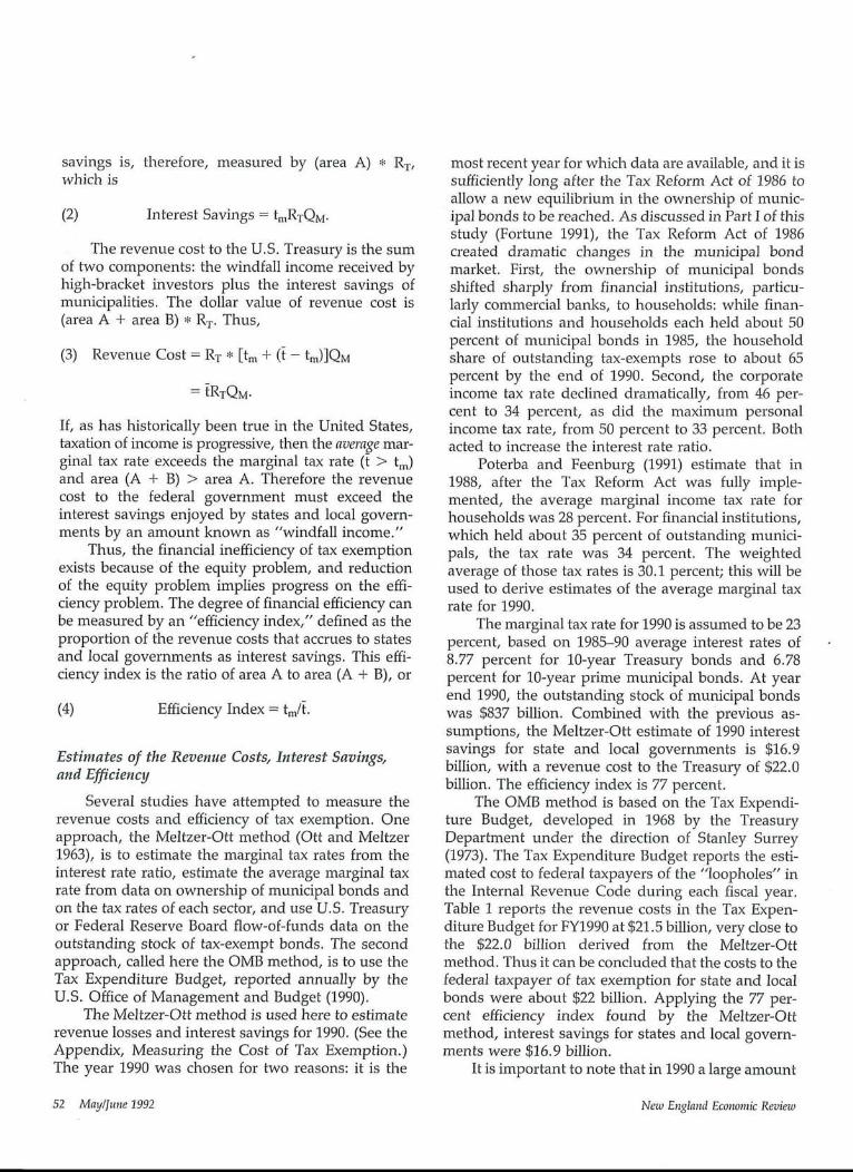
The OMB method is based on the Tax Expendi-ture Budget, developed in 1968 by the TreasuryDepartment under the direction of Stanley Surrey(1973). The Tax Expenditure Budget reports the esti-mated cost to federal taxpayers of the "loopholes" inthe Internal Revenue Code during each fiscal year.Table 1 reports the revenue costs in the Tax Expen-diture Budget for FY1990 at $21.5 billion, very close tothe $22.0 billion derived from the Meltzer-Ottmethod. Thus it can be concluded that the costs to thefederal taxpayer of tax exemption for state and localbonds were about $22 billion. Applying the 77 per-cent efficiency index found by the Meltzer-Ottmethod, interest savings for states and local govern-ments were $16.9 billion.

It is important to note that in 1990 a large amount

52 May/June 1992 New England Economic Review

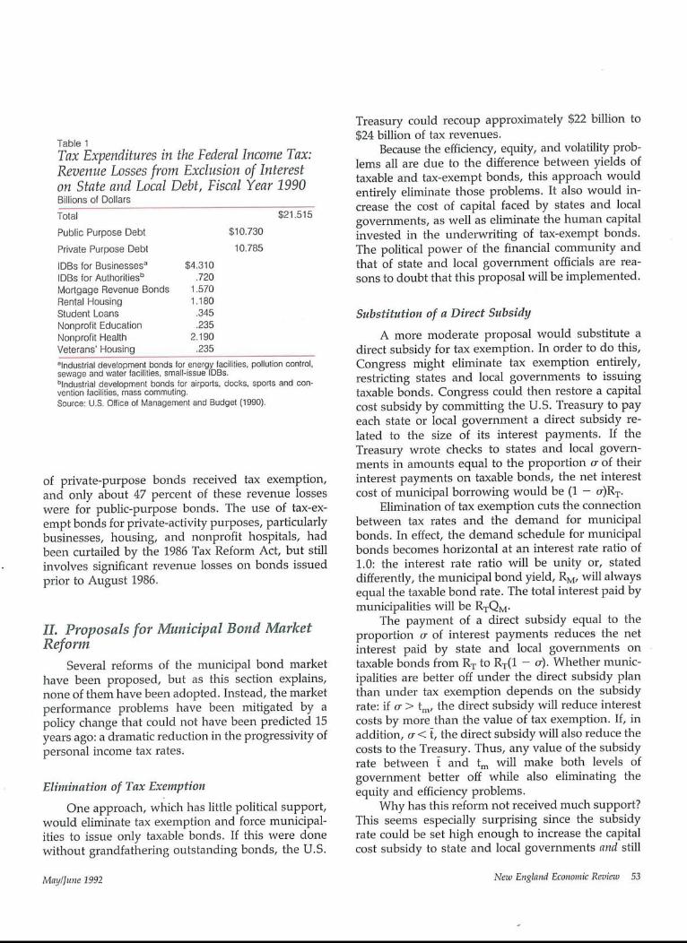
Table 1Tax Expenditures in the Federal Income Tax:Revenue Losses from Exclusion of Intereston State and Local Debt, Fiscal Year 1990Billions of Dollars~t~al - $21.515

$10.730

10.785Public Purpose Debt

Private Purpose Debt

IDBs for Businessesa $4.310IDBs for Authoritiesb .720Mortgage Revenue Bonds 1.570Rental Housing 1.180Student Loans .345Nonprofit Education .235Nonprofit Health 2.190Veterans’ Housing .235alndustrial development bonds for energy facilities, pollution control,sewage and water facilities, small-issue IDBs.blndustrial development bonds for airports, docks, sports and con-vention facilities, mass commuting.Source: U.S. Office of Management and Budget (1990).

of private-purpose bonds received tax exemption,and only about 47 percent of these revenue losseswere for public-purpose bonds. The use of tax-ex-empt bonds for private-activity purposes, particularlybusinesses, housing, and nonprofit hospitals, hadbeen curtailed by the 1986 Tax Reform Act, but stillinvolves significant revenue losses on bonds issuedprior to August 1986.

H. Proposals for Municipal Bond MarketReform

Several reforms of the municipal bond markethave been proposed, but as this section explains,none of them have been adopted. Instead, the marketperformance problems have been mitigated by apolicy change that could not have been predicted 15years ago: a dramatic reduction in the progressivity ofpersonal income tax rates.

Elimination of Tax Exemption

One approach, wlitich has little political support,would eliminate tax exemption and force municipal-ities to issue only taxable bonds. If this were donewithout grandfathering outstanding bonds, the U.S.

Treasury could recoup approximately $22 billion to$24 billion of tax revenues.

Because the efficiency, equity, and volatility prob-lems all are due to the difference between yields oftaxable and tax-exempt bonds, this approach wouldentirely eliminate those problems. It also would in-crease the cost of capital faced by states and localgovernments, as well as eliminate the human capitalinvested in the underwriting of tax-exempt bonds.The political power of the financial community andthat of state and local government officials are rea-sons to doubt that this proposal will be implemented.

Substitution of a Direct Subsidy

A more moderate proposal would substitute adirect subsidy for tax exemption. In order to do this,Congress might eliminate tax exemption entirely,restricting states and local governments to issuingtaxable bonds. Congress could then restore a capitalcost subsidy by committing the U.S. Treasury to payeach state or local government a direct subsidy re-lated to the size of its interest payments. If theTreasury wrote checks to states and local govern-ments in amounts equal to the proportion cr of theirinterest payments on taxable bonds, the net interestcost of municipal borrowing would be (1 - o’)RT.

Elimination of tax exemption cuts the connectionbetween tax rates and the demand for municipalbonds. In effect, the demand schedule for municipalbonds becomes horizontal at an interest rate ratio of1.0: the interest rate ratio will be unity or, stateddifferently, the municipal bond yield, RM, will alwaysequal the taxable bond rate. The total interest paid bymunicipalities will be RTQM.

The payment of a direct subsidy equal to theproportion o- of interest payments reduces the netinterest paid by state and local governments ontaxable bonds from RT to RT(1 -- ~r). Whether munic-ipalities are better off under the direct subsidy planthan under tax exemption depends on the subsidyrate: if o- > tm, the direct subsidy will reduce interestcosts by more than the value of tax exemption. If, inaddition, o- < ~, the direct subsidy will also reduce thecosts to the Tre_asury. Thus, any value of the subsidyrate between t and tm will make both levels ofgovernment better off while also eliminating theequity and efficiency problems.

Why has this reform not received much support?This seems especially surprising since the subsidyrate could be set high enough to increase the capitalcost subsidy to state and local governments and still

May/June 1992 New England Economic Review 53

reduce the costs to federal taxpayers. The oppositioncomes from several sources. First, high-income inves-tors do not want to see their windfalls eliminated; thishas been particularly true since the 1986 Tax ReformAct, which eliminated many other tax shelters. Sec-ond, state and local governments fear that a directsubsidy is the first step toward elimination of anysubsidy: after adopting a direct subsidy, Congressmight either eliminate it or drastically reduce thesubsidy rate, leaving states and municipalities with amuch-reduced subsidy in the future. Finally, thesecurities industry--particularly that portion in-volved in underwriting and trading municipalbonds--has lobbied vigorously against any changesin tax exemption because municipal bond underwrit-ers, traders, and attorneys do not eagerly accept theconsequences.

The Taxable Bond Option

A complete elimination of tax exemption,whether or not accompanied by a direct subsidy, isnot in the political cards. This leads to considerationof a reform that combines aspects of the currentsystem and of taxable bonds with a direct subsidy.This is the taxable bond option, which was initiallyproposed in the 1940s as a method of eliminatingtax-exempt securities (Seltzer 1941) and received con-siderable attention in the early 1970s (Galper andPetersen 1971, Fortune 1973a and 1973b, Huefner1971).

The taxable bond option would give state andlocal governments the option to issue either taxable ortax-exempt bonds. In order to provide an incentive toissue bonds in the taxable form, a direct subsidylinked to the interest costs of taxable municipal bondswould be paid to the issuing government. In order toinduce municipalities to issue taxable bonds, thesubsidy rate must exceed the tax rate of the marginalinvestor in tax-exempts in the current regime: ifo- < tin, the taxable bond option would not be chosen,because municipalities would be better off issuingtax-exempt bonds at a rate of RT(1 -- tin) than taxablebonds at a net rate of RT(1 -- ~r). Only if rr exceeded tmwould municipalities have an incentive to issue tax-able bonds at the margin. But as municipalities sub-stituted taxable bonds for tax-exempts, the volume oftax-exempt bonds would decline and the tax rate ofthe marginal investor in tax-exempts would increase.If the subsidy rate is less than the maximum tax rate(tm~), the market will settle down to a new equilib-rium with municipal bonds issued in both taxable and

tax-exempt forms. In this new equilibrium, the newmarginal investor’s tax rate will be equal to thesubsidy rate (tin = o’) because municipalities willadjust the composition of their debt so that, at themargin, taxable and tax-exempt bonds carry equal netinterest costs.

Consider Figure 4, a replica of Figure 3 with animportant reinterpretation. The DD schedule is nowthe demand schedule for tax-exempt bonds, so thehorizontal distance from the vertical axis to DDshows the amount of tax-exempt bonds that will bedemanded at each interest rate ratio. The supplyschedule SS shows the amount of total municipaldebt--taxable and tax-exempt--that will be outstand-ing. Thus, at each rate ratio, the horizontal distancefrom DD to SS represents the amount of taxable bondsissued.

Figure 4 assumes a subsidy rate on taxable bondsexceeding the subsidy via tax exemption (o- > t~).The introduction of the taxable bond option results ina kinked supply schedule for tax-exempt bonds. Atany interest rate ratio less than (1 - o-), municipalitieswill issue only tax-exempts, so that SS is the supplyschedule for tax-exempts when RM < (1 - o’)RT. For

Figure 4

mM

1.0

(1-tm)

(1-tmax)

The Taxable Bond Option

C1

A2

B2C2

QM

Outstanding Stockof Municipal Bonds

54 May/June 1992 New England Economic Review

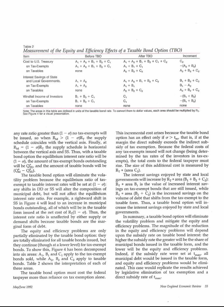
Table 2Mea_surement of the Equity and E~ciency Effects of aItem Before TBO

Cost to U.S. Treasury A1 + A2 + B1 4- B2 4- 01 A1on Tax-Exempts A1 + A2 + B~ + B2 + Cl A~

on Taxables none A2

Taxable Bond Optio~z (TBO~)_" -,~ft~r TBO Increment

+ A2 + B~ + B2 + C1 + C2 C2

+ B~ + C~ -(A2 + B2)4- B2 + C2

A2 + B2 + C2

Interest Savings of Stateand Local Governments. A~ + A2 A1 + A2 + B~ + B2 + C2 B1 + B2 + C2

on Tax-Exempts A1 + A2 A~ + B~ B~ - A2on Taxables none A2 + B2 + C2 A2 + B2 + C2

Windfall Income of Investors B~ + B2 + C~ C~ -(B~ 4- B2)on Tax-Exempts B1 + B2 + C~ C~ -(B1 + B2)on Taxables none none none

Note: The areas in this table are defined in units of the taxable bond rate. To convert them to dollar values, each area should be multiplied by RT.See Figure 4 for a visual presentation.

any rate ratio greater than (1 - o-) no tax-exempts willbe issued, so when RM > (1 - o’)RT the supplyschedule coincides with the vertical axis. Finally, atRM = (1 - o’)RT the supply schedule is horizontalbetween the vertical axis and SS. Thus, with a taxablebond option the equilibrium interest rate ratio will be(1 - o-), the amount of tax-exempt bonds outstandingwill be Q~E, and the amount of taxable bonds will be(Q~ - Q~E)"

The taxable bond option will eliminate the vola-tility problem because the equilibrium ratio of tax-exempt to taxable interest rates will be set at (1 - ~r):any shifts in DD or SS will alter the composition ofmunicipal debt, but will not affect the equilibriuminterest rate ratio. For example, a rightward shift inSS in Figure 4 will lead to an increase in municipalbonds outstanding, all of which will be in the taxableform issued at the net cost of RT(1 -- ~). Thus, theinterest rate ratio is unaffected by either supply ordemand shifts because taxable bonds are the mar-ginal form of debt.

The equity and efficiency problems are onlypartially eliminated by the taxable bond option: theyare totally eliminated for all taxable bonds issued, butthey continue (though at a lower level) for tax-exemptbonds. To show this, Figure 4 has been decomposedinto six areas: A1, B~ and C~ apply to the tax-exemptbonds sold, while A2, B2 and C2 apply to taxablebonds. Table 2 shows the interpretation of each ofthese areas.

The taxable bond option must cost the federaltaxpayer more than reliance on tax exemption alone.

This incremental cost arises because the taxable bondoption has an effect only if o- > tm, that is, if at themargin the direct subsidy exceeds the indirect sub-sidy of tax exemption. Because the federal costs ofany tax-exempts issued will not change (being deter-mined by the tax rates of the investors in tax-ex-empts), the total costs to the federal taxpayer mustrise. The size of this additional cost is measured byRT * (area C2).

The interest savings enjoyed by state and localgovernments will increase by RT * area (B1 + B2 + C2):RT * area B~ is the value of increased interest sav-ings on tax-exempt bonds that are still issued, whileRT * area (B2 + C2) is the increased savings on thevolume of debt that shifts from the tax-exempt to thetaxable form. Thus, a taxable bond option will in-crease the interest savings enjoyed by state and localgovernments.

In summary, a taxable bond option will eliminatethe volatility problem and mitigate the equity andefficiency problems. The magnitude of the reductionin the equity and efficiency problems will dependupon the subsidy rate on taxable bond interest: thehigher the subsidy rate the greater will be the share ofmunicipal bonds issued in the taxable form, and thelower will be the equity and efficiency problems.Indeed, if the subsidy rate were set at tr~, allmunicipal debt would be issued in the taxable form,and equity and efficiency problems would be elimi-nated. This case would replicate the results achievedby legislative elimination of tax exemption and adirect subsidy rate of tmax.

May/June 1992 New England Economic Review 55

The taxable bond option is clearly a compromise,which maintains tax exemption but also inducesmunicipalities to issue taxable bonds. It has beenopposed by the same groups that have opposed themore extreme reform of completely eliminating taxexemption and replacing it with a direct subsidy ontaxable municipal bonds. While the opposition hasbeen a bit less monolithic--with, for example, lessconcerted opposition among municipal finance offi-cials--it has been sufficiently vigorous to preventadoption of the taxable bond option.

A Flat Income Tax

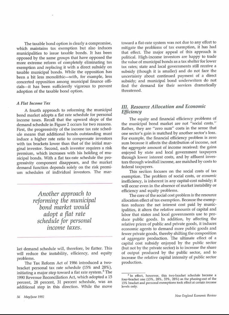
A fourth approach to reforming the municipalbond market adopts a flat rate schedule for personalincome taxes. Recall that the upward slope of thedemand schedule in Figure 2 occurs for two reasons.First, the progressivity of the income tax rate sched-ule means that additional bonds outstanding mustinduce a higher rate ratio to compensate investorswith tax brackets lower than that of the initial mar-ginal investor. Second, each investor requires a riskpremium, which increases with his holding of mu-nicipal bonds. With a flat tax-rate schedule the pro-gressivity component disappears, and the marketdemand function depends solely on the risk premi-um schedules of individual investors. The mar-

Another approach toreforming the municipal

bond market wouldadopt a fiat rate

schedule for personalincome taxes.

ket demand schedule will, therefore, be flatter. Thiswill reduce the instability, efficiency, and equityproblems.

The Tax Reform Act of 1986 introduced a two-bracket personal tax rate schedule (15% and 28%),initiating a major step toward a flat rate system.5 The1990 Revenue Reconciliation Act, which adopted a 15percent, 28 percent, 31 percent schedule, was anadditional step in this direction. While the move

toward a flat-rate system was not due to any effort tomitigate the problems of tax exemption, it has hadthat effect. The major appeal of this approach ispolitical. High-income investors are happy to tradethe value of municipal bonds as a tax shelter for lowertax rates; state and local governments still receive asubsidy (though it is smaller) and do not face theuncertainty about continued payment of a directsubsidy; and municipal bond underwriters do notfind the demand for their services dramaticallythreatened.

IlL Resource Allocation and EconomicEfficiency

The equity and financial efficiency problems ofthe municipal bond market are not "social costs."Rather, they are "zero sum" costs in the sense thatone sector’s gain is matched by another sector’s loss.For example, the financial efficiency problem is zerosum because it affects the distribution of income, notthe aggregate amount of income received: the gainsenjoyed by state and local government taxpayersthrough lower interest costs, and by affluent inves-tors through windfall income, are matched by costs tofederal taxpayers.

This section focuses on the social costs of taxexemption. The problem of social costs, or economicinefficiency, is inherent in any capital-cost subsidy; itwill occur even in the absence of market instability orefficiency and equity problems.

The core of the social cost problem is the resourceallocation effect of tax exemption. Because the exemp-tion reduces the net interest cost paid by munic-ipalities, it alters the relative amounts of capital andlabor that states and local governments use to pro-duce public goods. In addition, by affecting therelative prices of public and private goods, it induceseconomic agents to demand more public goods andfewer private goods, thereby shifting the compositionof aggregate production. The ultimate effect of acapital cost subsidy enjoyed by the public sector(but not by the private sector) is to increase the shareof output produced by the public sector, and toincrease the relative capital intensity of public sectorproduction.

s In effect, however, this two-bracket schedule became afour-bracket one (15%, 28%, 33%, 28%) as the phasing-out of the15% bracket and personal exemptions took effect at certain incomelevels only.

56 May/June 1992 New England Economic Review

The Microeconomics of Economic Efficiency

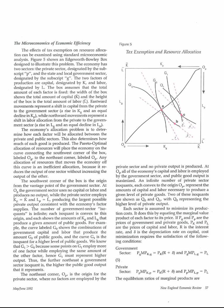
The effects of tax exemption on resource alloca-tion can be examined using standard microeconomicanalysis. Figure 5 shows an Edgeworth-Bowley Boxdesigned to illustrate this problem. The economy hastwo sectors: the private sector, designated by the sub-script "p", and the state and local government sector,designated by the subscript "g". The two factors ofproduction are capital, designated by K, and labor,designated by L. The box assumes that the totalamount of each factor is fixed: the width of the boxshows the total amount of capital (I~) and the heightof the box is the total amount of labor (L). Eastwardmovements represent a shift in capital from the privateto the government sector (a rise in Kg and an equaldecline in Kp), while northward movements represent asl~ift in labor allocation from the private to the govern-ment sector (a rise in Lg and an equal decline in Lp).

The economy’s allocation problem is to deter-mine how each factor will be allocated between theprivate and public sectors. This also determines howmuch of each good is produced. The Pareto-Optimalallocation of resources will place the economy on thecurve connecting the southwest corner of the box,labeled Og, to the northeast corner, labeled Op. Anyallocation of resources that moves the economy offthis curve is an inefficient allocation, because it re-duces the output of one sector without increasing theoutput of the other.

The southwest corner of the box is the originfrom the vantage point of the government sector. AtOg the government sector uses no capital or labor andproduces no output, while the private sector employsKp = I~ and Lp = J~, producing the largest possibleprivate output consistent with the economy’s factorsupplies. The number of government-sector "iso-quants" is infinite; each isoquant is convex to thisorigin, and each shows the amounts of Kg and Lg thatproduce a given amount of public goods. For exam-ple, the curve labeled GO shows the combinations ofgovernment capital and labor that produce theamount Go of public goods, and the curve G1 is theisoquant for a higher level of public goods. We knowthat G1 > Go because some points on G1 employ moreof one factor while employing the same amount ofthe other factor, hence G1 must represent higheroutput. Thus, the further northeast a governmentsector isoquant is, the higher the public good outputthat it represents.

The northeast corner, Op, is the origin for theprivate sector, where no factors are employed by the

Figure 5

Tax Exen~ption and Resource Allocation

L

K

61

L

private sector and no private output is produced. AtOp all of the economy’s capital and labor is employedby the government sector, and public good output ismaximized. An infinite number of private sectorisoquants, each convex to the origin Op, represent theamounts of capital and labor necessary to produce agiven level of private goods. Two of these isoquantsare shown as Q0 and Q1, with Q0 representing thehigher level of private output.

Each sector is assumed to minimize its produc-tion costs. It does this by equating the marginal valueproduct of each factor to its price. If Pg and Pp are theprices of government and private goods, PK and PL

are the prices of capital and labor, R is the interestrate, and 3 is the depreciation rate on capital, costminimization requires the satisfaction of the follow-ing conditions:

GovernmentSector: PgMPK,g = PK(R ÷ 3) and PgMPL,g = PL

(5)Private

Sector: PpMPK,p = PK(R + 3) and PpMPL,p = PL

The equilibrium ratios of marginal products are

May/June 1992 New England Economic Review 57

Government Sector:

(6)Private Sector:

MPK,g/MPL, g = [PK(R + 6)]/PL

MPK,p/MPL,p = [PK(R + 6)]/PL

The marginal product ratios for each sector arerepresented by the slope of the isoquant for thatsector. Because both sectors face the same factorprices, each sector will be induced to choose factorcombinations that have the same marginal productratios, that is, the same isoquant slopes. As notedabove, the line connecting Og and Op is composed ofall the points that represent an efficient allocation ofresources. This line also turns out to be all the pointsat which the isoquants are tangent and, therefore,have equal slopes.

For example, consider point a, assumed to be thepoint at which the economy rests before introductionof tax exemption. At point a the isoquant Go istangent to the isoquant Qo. Any other point on GOwill, because of the shapes of the isoquants, be on alower (more northeasterly) private-sector isoquantthan Qo. Thus, any movement away from a giveslower private output for the same level of govern-ment output. The result is economic inefficiency,because the level of private output is lower thannecessary to produce GO of public output.

In order to investigate the effects of tax exemp-tion, assume that the economy is initially in a generalequilibrium at point a, and that both sectors pay thesame user cost of capital and wage rate. At this initialgeneral equilibrium, the economy is Pareto-Efficient.If tax exemption is introduced, and the interest ratepaid by the government sector, RM, is below the ratepaid by the private sector, RT, then the relative factorcosts for governments will be PK(RM + i~)/Vq, mea-sured on the box by the angle/_2. The private sectorstill faces the same factor price ratio, measured by/_1,so it wishes to remain at point a. But the governmentsector would want to move to point b, which mini-mizes the cost of producing Go of output under thenew factor cost ratio.

Tax exemption has thrown the economy intodisequilibrium: the private sector wants to use theamount of capital and labor represented by point a,leaving the government sector only I~ - Kp of capitaland 1~ - Lg of labor. In the initial equilibrium that wasprecisely the amount of capital and labor that thegovernment sector wanted to use. But now the gov-ernment wants to use more capital and less labor. Inshort, the introduction of tax exemption creates anexcess demand for capital and an excess supply oflabor. Furthermore, tax exemption has driven a per-

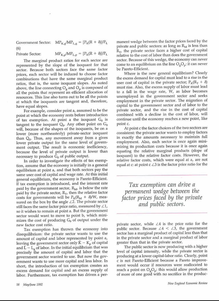
manent wedge between the factor prices faced by theprivate and public sectors: as long as RM is less thanRT, the private sector faces a higher cost of capitalrelative to the cost of labor than does the governmentsector. Because of this wedge, the economy can nevercome to an equilibrium on the line OgOp: it can neverbe Pareto-Efficient.

Where is the new general equilibrium? Clearlythe excess demand for capital must lead to a rise in theuser cost of capital in the private sector; PK(RT + 6)must rise. Also, the excess supply of labor must leadto a fall in the wage rate, W, as labor becomesunemployed in the government sector and seeksemployment in the private sector. The migration ofcapital to the government sector and of labor to theprivate sector, and the rise in the cost of capitalcombined with a decline in the cost of labor, willcontinue until the economy reaches a new point, likepoint c.

At point c the factor choices of the two sectors areconsistent: the private sector wants to employ factorsin exactly the amounts necessary to maintain fullemployment. Also, each sector is once again mini-mizing its production costs because it is once againequating the relative marginal products (slope ofisoquant) to the relative factor costs. However, therelative factor costs, which were equal at a, are notequal at c: at point c/_3 is the factor price ratio for the

Tax exemption can drive apermanent wedge between the

factor prices faced by the privateand public sectors.

private sector, while /_4 is the price ratio for thepublic sector. Because /_4 < /-3, the governmentsector has a marginal product of capital less than thatin the private sector and a marginal product of laborgreater than that in the private sector.

The public sector is now producing with a higherlevel of capital intensity, while the private sector isproducing at a lower capitaMabor ratio. Clearly, pointc is not Pareto-Efficient because a Pareto improve-ment would occur if resources were reallocated toreach a point on OgOp: this would allow productionof more of one good with no sacrifice in the produc-

58 .May/June 1992 New England Economic Reviezo

tion of the other good. But the price system will notinduce that movement; the government has a perma-nent incentive to produce with too much capital andtoo little labor.

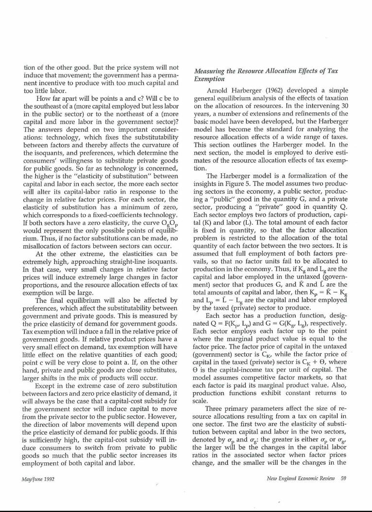
How far apart will be points a and c? Will c be tothe southeast of a (more capital employed but less laborin the public sector) or to the northeast of a (morecapital and more labor in the government sector)?The answers depend on two important consider-ations: technology, which fixes the substitutabilitybetween factors and thereby affects the curvature ofthe isoquants, and preferences, which determine theconsumers’ willingness to substitute private goodsfor public goods. So far as technology is concerned,the higher is the "elasticity of substitution" betweencapital and labor in each sector, the more each sectorwill alter its capital-labor ratio in response to thechange in relative factor prices. For each sector, theelasticity of substitution has a minimum of zero,which corresponds to a fixed-coefficients technology.If both sectors have a zero elasticity, the curve OgOpwould represent the only possible points of equilib-rium. Thus, if no factor substitutions can be made, nomisallocation of factors between sectors can occur.

At the other extreme, the elasticities can beextremely high, approaching straight-line isoquants.In that case, very small changes in relative factorprices will induce extremely large changes in factorproportions, and the resource allocation effects of taxexemption will be large.

The final equilibrium will also be affected bypreferences, which affect the substitutability betweengovernment and private goods. This is measured bythe price elasticity of demand for government goods.Tax exemption will induce a fall in the relative price ofgovernment goods. If relative product prices have avery small effect on demand, tax exemption will havelittle effect on the relative quantities of each good;point c will be very close to point a. If, on the otherhand, private and public goods are close substitutes,larger shifts in the mix of products will occur.

Except in the extreme case of zero substitutionbetween factors and zero price elasticity of demand, itwill always be the case that a capital-cost subsidy forthe government sector will induce capital to movefrom the private sector to the public sector. However,the direction of labor movements will depend uponthe price elasticity of demand for public goods. If thisis sufficiently high, the capital-cost subsidy will in-duce consumers to switch from private to publicgoods so much that the public sector increases itsemployment of both capital and labor.

Measuring the Resource Allocation Effects of TaxExemption

Arnold Harberger (1962) developed a simplegeneral equilibrium analysis of the effects of taxationon the allocation of resources. In the intervening 30years, a number of extensions and refinements of thebasic model have been developed, but the Harbergermodel has become the standard for analyzing theresource allocation effects of a wide range of taxes.This section outlines the Harberger model. In thenext section, the model is employed to derive esti-mates of the resource allocation effects of tax exemp-tion.

The Harberger model is a formalization of theinsights in Figure 5. The model assumes two produc-ing sectors in the economy, a public sector, produc-ing a "public" good in the quantity G, and a privatesector, producing a "private" good in quantity Q.Each sector employs two factors of production, capi-tal (K) and labor (L). The total amount of each factoris fixed in quantity, so that the factor allocationproblem is restricted to the allocation of the totalquantity of each factor between the two sectors. It isassumed that full employment of both factors pre-vails, so that no factor units fail to be allocated toproduction in the economy. Thus, if Kg and Lg are thecapital and labor employed in the untaxed (govern-ment) sector that produces G, and I~ and l~ are thetotal amounts of capital and labor, then Kp = I~ - Kgand Lp = I~ - Lg are the capital and labor employedby the taxed (private) sector to produce.

Each sector has a production function, desig-nated Q = F(Kp, Lp) and G = G(Kg, Lg), respectively.Each sector employs each factor up to the pointwhere the marginal product value is equal to thefactor price. The factor price of capital in the untaxed(government) sector is CK, while the factor price ofcapital in the taxed (private) sector is CK + ~9, whereO is the capital-income tax per unit of capital. Themodel assumes competitive factor markets, so thateach factor is paid its marginal product value. Also,production functions exhibit constant returns toscale.

Three primary parameters affect the size of re-source allocations resulting from a tax on capital inone sector. The first two are the elasticity of substi-tution between capital and labor in the two sectors,denoted by o-p and o-g: the greater is either O’p or ~g,the larger will be the changes in the capital laborratios in the associated sector when factor priceschange, and the smaller will be the changes in the

May/June 1992 Nao England Economic Review 59

relative factor prices associated with changes in factorcomposition. This follows the general principle thatthe closer the substitutability between any two com-modities, the larger will be the response in the ratio ofthe quantities used to any relative price change.Thus, a given change in relative quantities can beachieved by a smaller relative price change when twocommodities are close substitutes.

The third primary parameter is the price elastic-ity of demand for the public good, Eg. The higher thisprice elasticity, the larger will be the shift in theallocation of the consumers’ consumption bundle inresponse to any change in relative prices; for anygiven change in relative prices, the shift in demandbetween the taxed and untaxed sectors is greaterwhen the goods are closer substitutes.

Estimates of the Effects of Tax Exemption

To estimate the resource allocation effects of taxexemption, it is necessary to assume values for theprimary parameters, discussed above, which describethe response of economic agents to changes in rela-tive prices. In addition, values must be assigned toseveral secondary parameters, which describe theallocation of resources in the economy. Among theseare the capital income shares in each sector (fK andgK), the initial ratio of government sector capital toprivate sector capital (~K) and the initial ratio ofgovernment labor to private labor (~C).

The appropriate values of these secondary pa-rameters will depend upon the definition of theprivate sector. Is it defined as nonfinancial corpora-tions, all corporations, or all businesses includingunincorporated enterprises? Does it include produc-tion of housing services? of farm output? The privatesector has no single definition; here it has beendefined to include all private nonagricultural produc-tion of goods and services except housing.

The U.S. Bureau of Labor Statistics establishmentsurveys of nonagricultural payrolls show that in the1980-85 period there were 17.4 state and local sectoremployees for every 100 private sector employees;hence /~L = 0.174. The U.S. Commerce Department’scapital stock estimates (Musgrave 1990) indicate thatin the 1982-89 period there was an average of $40.50of state and local sector capital for every $100 of fixednonresidential capital stock; hence, ~K = 0.405.

According to Hulten and Schwab (1987), in the1980-85 period about 24 percent of the value added inthe state and local government sector was due to theservices of the capital stock, hence gK = 0.24. The

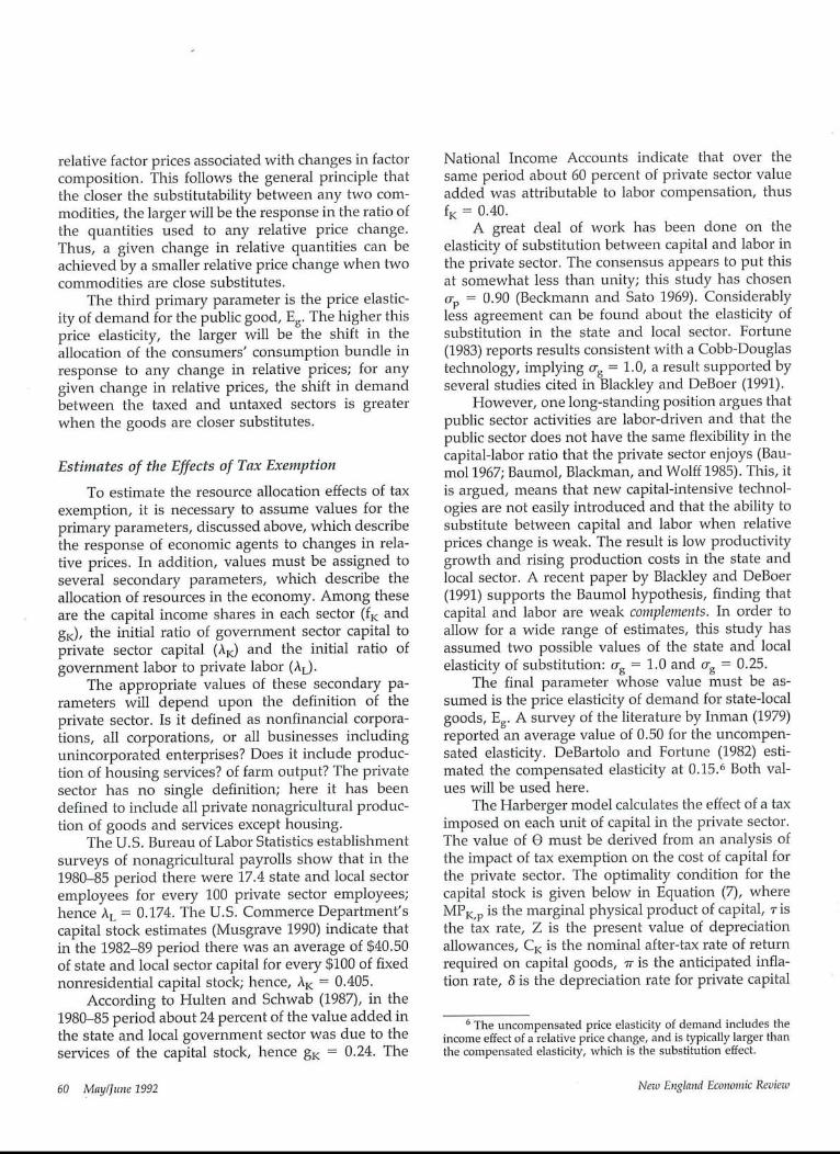
National Income Accounts indicate that over thesame period about 60 percent of private sector valueadded was attributable to labor compensation, thusfK = 0.40.

A great deal of work has been done on theelasticity of substitution between capital and labor inthe private sector. The consensus appears to put thisat somewhat less than unity; this study has chosenCrp = 0.90 (Beckmann and Sato 1969). Considerablyless agreement can be found about the elasticity ofsubstitution in the state and local sector. Fortune(1983) reports results consistent with a Cobb-Douglastechnology, implying Crg = 1.0, a result supported byseveral studies cited in Blackley and DeBoer (1991).

However, one long-standing position argues thatpublic sector activities are labor-driven and that thepublic sector does not have the same flexibility in thecapitaMabor ratio that the private sector enjoys (Bau-mo11967; Baumol, Blackman, and Wolff 1985). This, itis argued, means that new capital-intensive technol-ogies are not easily introduced and that the ability tosubstitute between capital and labor when relativeprices change is weak. The result is low productivitygrowth and rising production costs in the state andlocal sector. A recent paper by Blackley and DeBoer(1991) supports the Baumol hypothesis, finding thatcapital and labor are weak complements. In order toallow for a wide range of estimates, this study hasassumed two possible values of the state and localelasticity of substitution: crg = 1.0 and ~g = 0.25.

The final parameter whose value must be as-sumed is the price elasticity of demand for state-localgoods, Eg. A survey of the literature by Inman (1979)reported an average value of 0.50 for the uncompen-sated elasticity. DeBartolo and Fortune (1982) esti-mated the compensated elasticity at 0.15.6 Both val-ues will be used here.

The Harberger model calculates the effect of a taximposed on each unit of capital in the private sector.The value of (9 must be derived from an analysis ofthe impact of tax exemption on the cost of capital forthe private sector. The optimality condition for thecapital stock is given below in Equation (7), whereMPK,p is the marginal physical product of capital, ¯ isthe tax rate, Z is the present value of depreciationallowances, CK is the nominal after-tax rate of returnrequired on capital goods, w is the anticipated infla-tion rate, 6 is the depreciation rate for private capital

6 The uncompensated price elasticity of demand includes theincome effect of a relative price change, and is typically larger thanthe compensated elasticity, which is the substitution effect.

60 May/June 1992 New England Economic Review

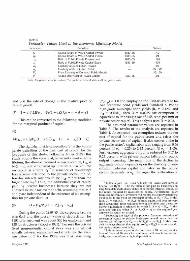
Table 3P~a2"ame_te_.r Valu_es Used in the E~o~no__m_i_.c__Efficiency Mode_l_Parameter

f<gK~’K

Eg

Note: The private sector is

Definition

Capital Share of Value Added, Private 198045Capital Share of Value Added, Public 1980-85Ratio of Public/Private Employment 1980-85Ratio of Public/Private Capital Stock 198249Elasticity of Substitution, Private --Elasticity of Substitution, Public --Price Elasticity of Demand, Public Goods --Added User Cost of Private Capital 198045

non-farm The public sector is all state and local governments.

Values

.40.24.174.405.90

.25, 1.00.15, .5O

.03

and ~/is the rate of change in the relative price ofcapital goods.

(7) (1 - ~’)PpMPK,p = PK(1 -- ~’Z)[CK - ~" + 3 + ~].

This can be converted to the following conditionfor the marginal product of capital:

(8)

MPK, p = (PK/Pp)(1 -- ~-Z){[CK- (~" - 3 - ~)]/(1 - ~’)}.

The right-hand side of Equation (8) is the appro-priate definition of the user cost of capital for thepurposes of this study. Following Miller (1977) thisstudy adopts the view that, in security market equi-librium, the after-tax required return on capital, CK, isRT(1 -- ~-), so the "grossed up" pre-tax return requiredon capital is simply RT.7 If issuance of tax-exemptbonds were extended to the private sector, the be-fore-tax interest rate would be RM rather than thehigher rate RT.8 Thus, the additional cost of capitalpaid by private businesses because they are notallowed to issue tax-exempt debt, assuming that ~r, 3and 1’ are independent of the existence of tax exemp-tion for private debt, is:

(9) (9 = (PK/Pp)(1 - rZ)[RT -- RM].

During the period 1980-85, the corporate tax ratewas 0.46 and the present value of depreciation for$100 of investment was about $40 for equipment and$28 for structures (Kopcke 1981).9 Because the privatefixed nonresidential capital stock was split almostequally between equipment and structures, the aver-age value of Z for the 1980s was 0.34. Assuming

(PK/Pp) = 1.0 and employing the 1980-85 average forAaa corporate bond yields and Standard & Poor’shigh-grade municipal bond yields (Rw = 0.1267 andRM = 0.1002), then (9 = 0.0265: tax exemption isequivalent to imposing a tax of 2.65 cents per unit ofprivate sector capital. This analysis uses (9 = 0.03.

The assumed parameter values are reported inTable 3. The results of the analysis are reported inTable 4. As expected, tax exemption reduces the netcost of capital for the public sector and raises theprivate sector cost of capital. It also creates a rise inthe public sector’s capital-labor ratio ranging from 0.66percent (if Crg = 0.25) to 2.13 percent (if O-g = 1.00).Furthermore, aggregate output is reduced by 0.07 to0.23 percent, with private output falling and publicoutput increasing. The magnitude of the decline inaggregate output depends upon the elasticity of sub-stitution between capital and labor in the publicsector: the greater is O-g, the larger the reallocation of

7 Miller argues that firms will use the lowest-cost form offinance. Let RT (1 - r) be the interest rate paid by businesses onlong-term debt (with deductibility of corporate interest), and Re bethe return required by investors on equity. Furthermore, apartfrom risk differentials, investors will require that equity generate ayield equal to the yield on municipal bonds, so RE = RM. In thiscase, CK = min[RT(1 -- r), RM]. Because equity and debt are veryclose substitutes, firms will issue one or the other until a securitymarket equilibrium is achieved in which RT(1 -- r) = RM. In thiscase, one can use either RT or RM/(1 -- r) as the required pre-corporate tax return on capital.

8 Following the logic of the previous footnote, extension oftax-exempt bonds to private businesses would mean that theinterest cost of capital is CK = ndn[RM(1 - r), RM]. In this case,debt is always cheaper than equity, so CK = RM(1 -- r). As a result,the pre-tax interest cost is RM.

9 This assumes: a pre-tax discount rate of 10 percent, servicelives of five and 20 years for equipment and structures, respec-tively, and sum-of-years digits depreciation.

May/June 1992 New England Economic Review 61

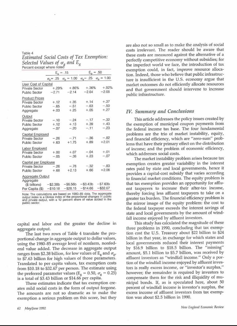
Table 4Estimated Social Costs of Tax Exemption:Selected Values of cr_ and EgPercent except where note~

Eg=.15 Eg=,50

O-g=.25 o-g= 1.00 %= .25 %= 1.00

User Cost of CapitalPrivate Sector +.29% +.86% +.36% +.92%Public Sector -2.71 -2.14 -2.64 -2.08

Product PricesPrivate Sector +.12 +.35 +.14 +.37Public Sector -.65 -.51 -.63 -.50Aggregate +.03 +.25 +.05 +.27

Private Sector -.10 -.24 -.17 -,32Public Sector +.12 +.13 +.39 +,43Aggregate -.07 -.20 -.11 -.23

Capital EmployedPrivate Sector -.26 -.71 -.36 -.82Public Sector +.63 +1.75 +.89 +2.01

Labor EmployedPrivate Sector +.00 +.07 -.04 +.01Public Sector -.05 -.38 +.23 -.07

Capital per EmployeePrivate Sector -.26 -.78 -.32 -.83Public Sector +.68 +2.13 +.66 +2.08

Ag.qre.qate OutputAggregate

($ billions) -$2.38b -$6.56b -$3.43b -$7.63bPer Capita ($) -$10.18 -$28.15 -$14.66 -$32.67

Note: The calculations are based on 1980q~5 data. The aggregateoutput index is a Divisia index of the proportional changes ~n publicand private output, with a 12 percent share of value added in lhepublic sector.

capital and labor and the greater the decline inaggregate output.

The last two rows of Table 4 translate the pro-portional change in aggregate output to dollar values,using the 1980-85 average level of nonfarm, nonfed-eral value added. The decrease in aggregate outputranges from $2.38 billion, for low values of Eg and %,to $7.63 billion for high values of those parameters.Translated to per capita values, tax exemption costsfrom $10.18 to $32.67 per person. The estimate usingthe preferred parameter values (Eg = 0.50, Crg = 0.25)is a total of $3.43 billion or $14.66 per capita.

These estimates indicate that tax exemption cre-ates mild social costs in the form of output forgone.The amounts are not so dramatic as to make theexemption a serious problem on this score, but they

are also not so small as to make the analysis of socialcosts irrelevant. The reader should be aware thatthese costs are measured against the alternative of aperfectly competitive economy without subsidies; forthe imperfect world we face, the introduction of taxexemption could, in fact, improve resource alloca-tion. Indeed, those who believe that public infrastruc-ture is insufficient in the U.S. economy argue thatmarket outcomes do not efficiently allocate resourcesand that government should intervene to increasepublic infrastructure.

IV. Summary and ConclusionsThis article addresses the policy issues created by

the exemption of municipal coupon payments fromthe federal income tax base. The four fundamentalproblems are the trio of market instability, equity,and financial efficiency, which are "zero-sum" prob-lems that have their primary effect on the distributionof income; and the problem of economic efficiency,which addresses social costs.

The market instability problem arises because taxexemption creates greater variability in the interestrates paid by state and local governments, hence itprovides a capital-cost subsidy that varies accordingto financial market conditions. The equity problem isthat tax exemption provides an opportunity for afflu-ent taxpayers to increase their after-tax income,thereby forcing less affluent taxpayers to take on agreater tax burden. The financial efficiency problem isthe mirror image of the equity problem: the cost tothe federal taxpayer exceeds the interest savings ofstate and local governments by the amount of wind-fall income enjoyed by affluent investors.

This study has calculated the magnitude of thesethree problems in 1990, concluding that tax exemp-tion cost the U.S. Treasury about $22 billion to $24billion in that year, in exchange for which states andlocal governments reduced their interest paymentsby $16.9 billion to $18.5 billion. The "missing"amount, $5.1 billion to $5.7 billion, was received byaffluent investors as "windfall income." Only a por-tion of the windfall income enjoyed by affluent inves-tors is really excess income, or "investor’s surplus,"however; the remainder is required by investors tocompensate them for the risk and illiquidity of mu-nicipal bonds. If, as is speculated here, about 50percent of windfall income is investor’s surplus, theexcess income of affluent investors from tax exemp-tion was about $2.5 billion in 1990.

62 .May/June 1992 New England Economic Review

This article also discusses several possible re-forms of the municipal bond market that wouldeliminate or mitigate the zero-sum problems. Thefirst is elimination of the exemption. The second is adirect subsidy, which would eliminate the exemptionbut replace it with federal payment of a portion ofstate and local government interest costs. The third isa taxable bond option, a combination of tax exemp-tion and a direct subsidy. None of these reforms havereceived sufficient political support, but the problemshave been mitigated by the major changes in the taxcode under the Tax Reform Act of 1986. The movetoward a flat income tax system has reduced the

magnitude of these problems.Finally, the article discusses the social costs of tax

exemption, which arise from the loss of output asresources are reallocated from the private sector tothe public sector in response to lower public sectorcapital costs. Using the period 1980-85 as the basis forestimates, this study concludes that in the 1980-85period the tax exemption reduced the annual aggre-gate output (value added) of the nonfarm, non-federal government sector by $2.4 billion to $7.6billion, depending on the assumptions. The preferredestimate is $3.4 billion, which translated to per capitaamounts equals $14.66 per person.

Appendix: Measuring

The U.S. Treasury Department used the Meltzer-Ottmethod in 1965 (Joint Economic Committee 1966) to calcu-late the interest savings and revenue costs on state andlocal bonds sold in 1965, over the lifetime of those bonds.The Treasury Department estimated an average marginaltax rate of 42 percent and a marginal tax rate of 28 percent.The interest savings over the lifetime of gross state andlocal bonds newly issued in 1965 were $1.9 billion, with arevenue cost of $2.9 billion. Using formula (4) above in thetext, these estimates imply an efficiency index of about 65percent.

These early Treasury estimates are incorrect becausethey rest on a confusion between average and marginalanalysis. The bonds sold in 1965 were incremental to thestock of outstanding municipal bonds, and the likely pur-chasers were the near-marginal investors in tax-exempts,whose windfall income would be very small. But the 1965application of the Meltzer-Ott method assumes that theincremental supply of bonds is bought by the averageinvestor, whose tax rate is measured by the average mar-ginal tax rate. The result is a potentially serious exaggera-tion of the costs of new bond issues. The method employedis, therefore, more suitable to estimation of the costs ofeliminating tax exemption for all outstanding bonds; in thiscase the average marginal tax rate is relevant.

The Meltzer-Ott method also makes some strong as-sumptions about market adjustments that occur in re-sponse to tax exemption. First, the method infers tax ratesfrom the existing pattern of ownership of municipal bonds,and assumes that in the absence of tax exemption thoseowners would simply have bought taxable bonds (includ-ing, of course, taxable municipals) to replace the no-longer-available tax-exempt bonds. Second, it assumes that thegeneral level of interest rates on taxable securities is notaffected by the existence of tax exemption. However, theadjustments that would occur if tax exemption did not existare far more complex than these assumptions suggest.

Consider the second point first. The effect of taxexemption on the taxable bond rate depends on the elas-ticity of the supply of both taxable and tax-exempt bonds.The Meltzer-Ott method assumes that either the outstand-ing stock of municipal debt is independent of interest rates(as, for convenience, is assumed in the text) or the private

the Cost of Tax Exemption

sector supply of debt is infinitely interest-elastic. In the firstcase, the introduction of tax exemption would inducegovernments to switch their issues from taxable to tax-exempt form, but investors would switch exactly thatamount of their portfolios to tax-exempts and out of taxablebonds. Because the shift in demand for taxable bonds (asinvestors switch from taxables to tax-exempts) is exactlymatched by the shift in the supply function (as govern-ments issue tax-exempts rather than taxable bonds), the netresult is no change in the taxable bond yield. In the secondcase, increased issues of municipal bonds in response to taxexemption "crowd out" an equal amount of taxable bonds,leaving the taxable bond yield unchanged.

If, in contrast to the assumption of the previous sec-tion, state and local governments respond to lower interestcosts by issuing more bonds, the introduction of tax exemp-tion will increase the quantity of loanable funds demandedand push up the general level of interest rates. As thishappens, private borrowers will reduce their bond issues inresponse to the higher costs. Only if the supply of privatetaxable bonds is infinitely interest-sensitive will the taxablebond rate remain unchanged; if not, the taxable bond ratemust go up.

Now consider the first point. The Meltzer-Ott methodassumes that investors simply switch from tax-exempts totaxable bonds, so that the pattern of ownership of out-standing tax-exempt bonds indicates the relevant tax ratesof those who would otherwise invest in taxable bonds.However, this need not be true. For example, suppose thattax exemption were eliminated for all outstanding munici-pal bonds and that current holders of tax-exempt bonds tryto shift into the next best tax shelter--common stocks. Inthis case, portfolio changes might create no additional taxesapart from temporary capital gains tax revenues. The neteffect on tax revenues will depend not on the tax rates ofinvestors who switch from tax-exempts to equities, butupon the tax rates of those who sold the equities andswitched into taxable bonds. Presumably these tax rates arelower than the rates of the former tax-exempt bondholdersbecause the equity sellers gave up the tax shelter of munic-ipal bonds. Thus, the method tends to overstate the rele-vant average marginal tax rate.

May/June 1992 New England Economic Review 63