the relationship of cloud cover to near-surface

1858 VOLUME 13J O U R N A L O F C L I M A T E

q 2000 American Meteorological Society

The Relationship of Cloud Cover to Near-Surface Temperature and Humidity:Comparison of GCM Simulations with Empirical Data

PAVEL YA. GROISMAN, RAYMOND S. BRADLEY, AND BOMIN SUN

Department of Geosciences, University of Massachusetts, Amherst, Massachusetts

(Manuscript received 11 January 1999, in final form 28 June 1999)

ABSTRACT

One of the possible ways to check the adequacy of the physical description of meteorological elements inglobal climate models (GCMs) is to compare the statistical structure of these elements reproduced by modelswith empirical data from the world climate observational system. The success in GCM development warranteda further step in this assessment. The description of the meteorological element in the model can be consideredadequate if, with a proper reproduction of the mean and variability of this element (as shown by the observationalsystem), the model properly reproduces the internal relationships between this element and other climatic variables(as observed during the past several decades). Therefore, to distinguish more reliable models, the authors suggestfirst analyzing these relationships, ‘‘the behavior of the climatic system,’’ using observational data and thentesting the GCMs’ output against this behavior.

In this paper, the authors calculated a set of statistics from synoptic data of the past several decades andcompared them with the outputs of seven GCMs participating in the Atmospheric Model Intercomparison Project(AMIP), focusing on cloud cover, one of the major trouble spots for which parameterizations are still not wellestablished, and its interaction with other meteorological fields. Differences between long-term mean values ofsurface air temperature and atmospheric humidity for average and clear sky or for average and overcast conditionscharacterize the long-term noncausal associations between these two elements and total cloud cover. Not all theGCMs reproduce these associations properly. For example, there was a general agreement in reproducing meandaily cloud–temperature associations in the cold season among all models tested, but large discrepancies betweenempirical data and some models are found for summer conditions. A correct reproduction of the diurnal cycleof cloud–temperature associations in the warm season is still a major challenge for two of the GCMs that weretested.

1. Introduction

Many meteorological phenomena that change rapidlyin time and space significantly affect the mean state ofthe climate system. Among these are cloud cover var-iations, which significantly (and immediately) alter theheat balance of the earth’s climate system on an hourlytime scale, but their effects are profound from seasonalthrough decadal timescales. Recent findings (Arking1991; Henderson-Sellers 1992; Kaas and Frich 1995;Abakumova et al. 1996) show that variations of cloudcover have significantly contributed to contemporaryclimatic changes. It is known that, on average, the pres-ence of clouds is associated with a cooler surface, butsignificant uncertainties are involved in assessing therole of cloudiness changes in the climate system underconditions related to increased greenhouse gases.Among these is the question: will cloud cover enhance

Corresponding author address: Dr. Pavel Groisman, UCAR ProjectScientist, National Climatic Data Center, 151 Patton Avenue, Ashe-ville, NC, 28801.E-mail: [email protected]

the process of climate changes (i.e., provide a positivefeedback) or will it dampen any changes (i.e., providea negative feedback)? Not all of these questions haveanswers today, and extensive international programs(e.g., GEWEX, ISLSCP, and ISCCP)1 targeting theseanswers are in progress. Two different approaches aregenerally used to address the feedback problems: mod-eling (Cess et al. 1991; Randall et al. 1994) and analysisof empirical data (Harrison et al. 1990; Gaffen and El-liott 1993; Groisman et al. 1994a,b, 1995, 1996, 1997).The efforts to match observational data, such as datafrom the Earth Radiation Budget Experiment (ERBE),with model output show large discrepancies among dif-ferent modeling groups (Cess et al. 1992a,b, 1993; Pot-ter et al. 1992; Wielicki et al. 1995). Modern GCMsparameterize effects of clouds differently and producea wide range of apparent ‘‘effects’’ of cloudiness on

1 Global Energy and Water Balance Experiment (GEWEX 1990),International Satellite Land Surface Climatology Project (Sellers etal. 1996), International Satellite Cloud Climatology Project (Rossowand Zhang 1995).

1 JUNE 2000 1859G R O I S M A N E T A L .

climate (Cess et al. 1991; Potter et al. 1992; Randall etal. 1994; Yao and Del Genio 1999). One conclusion iscertain from these model assessments, however: cloudcover is crucial for a proper assessment of the climaticsystem. Thus, uncertainty of cloud treatment in GCMsincreases by a factor of 2 the range of uncertainty offuture climate projections due to anthropogenic changesin greenhouse gases [Intergovernmental Panel on Cli-mate Change (IPCC) 1996]. To diminish this uncer-tainty, a proper physical description of cloudiness andits relationships with other meteorological elementsmust be developed. To claim that this description is‘‘proper,’’ we have to be sure that a package of physicalparameterizations in the model works on timescalesfrom diurnal to decadal and fully describes the behaviorof the contemporary climate system with variations incloudiness. We propose using modern observations tocheck the reality of this package by testing the rela-tionships between cloud cover2 and other meteorologicalelements.

2. Methodology

One of the possible ways to check the adequacy ofthe physical description of a meteorological element inthe model is to compare the statistical structure of thiselement (mean, standard deviation, and spatial and tem-poral correlation) reproduced by models with the em-pirical data of the world climate observational system(Stouffer et al. 1994; Weare and Mokhov 1995; DelGenio et al. 1996; Polyak 1996; Goody et al. 1998).Groisman et al. (1995, 1996) suggested a further stepin this assessment. The description of the meteorologicalelement in the model is considered adequate if, with aproper reproduction of the mean and variability of thiselement (as shown by the observational system), themodel properly reproduces the internal relationships be-tween this element and other climatic variables. Forexample, a correct description of cloud cover shouldinclude an appropriate change in the temperature fieldwhen clouds are changing and vice versa. This is gen-erally a more difficult task because instead of a properfit of mean values of each of these fields, a proper fitof a set of physical processes that manifest themselvesin interaction of these fields in the course of contem-porary climate variations is required. Sometimes in thepast, fits of the mean meteorological fields wereachieved artificially by changing the physical parame-

2 Cloud cover is only one of numerous characteristics of cloudiness.However, sufficiently long time series with information about othercloudiness characteristics available from national archives are scant,and the definitions of these characteristics vary with time and bycountry. Therefore, we were not able to secure the hemispheric cov-erage for other cloudiness characteristics for our analyses, and weuse only total cloud cover throughout this paper. Recent efforts byHahn and Warren (1999) indicate that this data paucity may soonchange.

ters of the GCMs from the solar constant to the depthof Hudson Bay. While due to such a ‘‘fitting’’ the cor-roboration with observations looks reasonable, the fu-ture use of these models for climate change studies be-came questionable. Beyond the present climate and pa-leoclimate reconstructions, each modeler group finds it-self in uncharted waters and must rely upon accuratereproductions by their model of the physical processesrather than rely upon specific meteorological fields (DelGenio et al. 1996).

Groisman et al. (1996) suggested using the followingstatistics for a set of climatic variables f to check thecorrect description of the interaction of element y withthese variables using empirical data:

OE(f | y ∈ D) 5 E(f) 2 E(f | y ∈ D), (1)

where E( ) is a mathematical expectation and E( | ) is aconditional expectation. We consider these statistics asa diagnostic vehicle that allows the description of ‘‘over-all effects’’ (OE) of the element y on the climate,3 andthus we allow a check of the proper reproduction ofthese effects by GCMs. The term ‘‘OE’’ was introducedby Groisman et al. (1996) with a clear indication thatdespite the name, these statistics do not represent causalrelationships or forcings but are bivariate associationsbetween internal climate variables (e.g., cloud cover andtemperature). Even the most vigorous proponent ofcloud forcing ideas will have difficulty explaining howclouds ‘‘force’’ a decrease in atmospheric pressure and/or an increase in wind speed near the surface. Yet chang-es in these variables are associated with the presence ofclouds (Groisman et al. 1996), as are many other chang-es, including those in humidity and temperature fields.Our OE estimates are not causal relationships but char-acterize an average state of these associations as a resultof numerous interactions within the climatic system. Wecontinue to use the term ‘‘overall effect’’ throughoutthis paper but warn against its interpretation as a causalrelationship.

To study the proper model description of the element‘‘u’’ when several other internal factors are involvedand contribute to the process under consideration, thefollowing statistic can be used:4

3 For example, if f is the top-of-the-atmosphere outgoing longwaveradiation (OLR) flux, y is cloudiness, and D corresponds to clear-skyconditions, we obtain the ‘‘cloud forcing’’ of OLR as defined byHarrison et al. (1990) from the ERBE data.

4 For example, if f is humidity, y is cloudiness, and D correspondsto clear-sky conditions, u is snow cover (a 5 snow-on-the-groundevents, and b 5 no-snow-on-the-ground events), and x is groundsurface temperature from a narrow range (C ), we get the effect ofthe presence of snow on the ground on humidity without contami-nation of this relationship by cloudiness and temperature variations(Groisman and Zhai 1995). When we want to exclude from consid-eration a contribution of a known factor, the POE statistics can beused as a supplementary tool.


POE(f | u | y ∈ D, x ∈ C)

5 E(f | u 5 a, y ∈ D, x ∈ C)

2 E(f | u 5 b, y ∈ D, x ∈ C), (2)

where POE is the partial overall effect.The class of Eqs. that (1) and (2) are in is wide and

not restricted by examples presented in the footnotesand throughout this paper. By introducing OE statistics,we suggest constructing a series of nontraditional cli-matologies (e.g., climatology of clear skies; climatologyof days with precipitation, with snow on the ground,and with calm conditions; and climatology of the weath-er along storm tracks) that differ distinctively from meanclimate conditions. The present behavior of the climaticsystem will be more prominently seen in these situationsthat are far from the average climate conditions because(1) the tails of any distribution generally contain moreinformation about that distribution than the values closeto its average state and (2) the assessment of the ‘‘dis-tinct’’ special conditions such as clear skies, calmweather, or the weather during precipitation events elu-cidates the relationships in the climatic system that pre-vail during these conditions and can be singled out andcompared with similar relationships in the GCMs’ out-put.

Mean monthly fields of the earth’s climatic systemremain quite stable, and their interannual variations con-stitute a small portion of weather variability in the time–space domain. It is possible to reconstruct these fieldswith a climate model that has incorrect parameters ordubious physics yet still do the reconstruction reason-ably well. Regretfully, if after such a verification themodel is applied to climatic change assessment, the re-sults will be unreliable. It is much better if the inter-annual variability of these fields and synoptic scale var-iability are well described by the model. In such cases,we can state that the model is consistent with modernclimate/weather variations and use it more confidentlyin experiments with changing external parameters (i.e.,in climate change studies).5 To distinguish more reliablemodels that correctly incorporate climate variability, wesuggest first analyzing this behavior using observationaldata for the past several decades and then testing theGCMs’ output behavior against nature. Only those thatpass this comparison are capable of delivering correctanswers in experiments with external forcing, and this

5 From this point of view, the Atmospheric Model IntercomparisonProject (AMIP) (Gates 1992; Gates et al. 1999) is a large-scale testof the internal consistency of the atmospheric circulation and theland–surface interaction schemes of the participating GCMs. Whencomparisons are made between the GCMs and empirical data, vari-ations of some meteorological fields (e.g., surface air temperature)are well reproduced by the AMIP runs (Gates et al. 1999) whereasother fields (cloudiness, soil moisture) are not (Weare and Mokhov1995; Robock et al. 1998).

(we hope) will narrow the present uncertainty in climatechange studies.

In this paper, we focus on one of the major troublespots, cloudiness, and its interaction within the climaticsystem where parameterizations are still not well de-termined. We will consider overall cloud effect (OCE)on surface air temperature (OCET) and atmospheric hu-midity (OCEH), defined either as temperature–humiditydifferences between average and clear sky weather con-ditions:

OCET

5 E(T ) 2 E(T | under clear sky conditions) (3)

and

OCEH

5 E(H ) 2 E(H | under clear sky conditions), (4)

where T is surface air temperature and H is a charac-teristic of the near-surface atmospheric humidity (watervapor pressure, e, and/or specific humidity, q, were usedthroughout this paper), or (in the humid tropics) as tem-perature–humidity differences between average andovercast weather conditions (subscript ‘‘1’’):

OCET1

5 E(T | under overcast conditions) 2 E(T ) (5)

and

OCEH1

5 E(H | under overcast conditions) 2 E(H ). (6)

Here, we change the sign in (5) and (6) to make itcomparable with (3) and (4).

We calculated Eqs. (3), (5), (4), and (6) without theconcern that observational practice at night significantlyinterferes with our estimates. The problem that we keepin mind here is obvious difficulties with nighttime ob-servations of cloudiness. To remedy this problem, Hahnet al. (1995) developed a moonlight criterion of cloud-iness observations. The essence of their analyses is thatthey filter the nighttime cloud observations and use onlythose that were made under enough brightness (e.g.,moonlight or twilight). This criterion significantly im-proved their nighttime cloudiness climatology, but ifused, it significantly reduces the sample size of thenighttime observations. Our analyses indicate that thisprecaution is not crucial (Sun and Groisman 2000; Sunet al. 2000, hereinafter SGBK).

It is possible to normalize the OCE and OCE1 to takeinto account the ‘‘distance’’ between clear, overcast, andaverage sky conditions by dividing the differences ineach meteorological element, f, by this distance. In thispaper, we chose not to do this because not much newinformation is generated with this normalization duringthe intercomparison of our empirical estimates of meandaily OCE with those derived from GCMs. Sun et al.(1999; SGBK) further investigate the questions related


FIG. 1. Map of stations that were used in this analysis. Dots rep-resent the stations with data delivered by the national meteorologicalservices. Triangles show the stations with data taken from the GlobalTelecommunication System and/or supplementary networks that haveless data than other stations in the region. The 36 stations in theSouthern Hemisphere (Indonesia and a few tropical islands) are notshown in this map.

to normalization and describe the temporal OCETchanges under contemporary climate conditions.

The appendixes describe several technical issues ofthe OCE estimation and the comparison of empiricalOCE estimates with those derived from GCM output.It also provides information about the accuracy of ourempirical OCET and OCEH estimates.

3. Data and model output used

In the comparison below, we used 1-h/3-h/6-h near-surface meteorological data from more than 1500 me-teorological stations distributed over the northern ex-tratropical land (NEL) area and the tropics for the pastseveral decades (Fig. 1). This dataset was described byGroisman et al. (1996), but then it was expanded withadditional stations from southern and central Europe,Canada, the United States (especially from Florida, Ha-waii, and the Pacific Islands), east Asia (China, Mon-golia, and Japan), and the tropics (Africa, Central Amer-ica, south and southeast Asia). The stations that areincluded in this dataset are reasonably well distributedover NEL, with a better than average coverage of theUnited States, Europe, eastern China, and the westernpart of the former USSR. This gives us an opportunityto calculate and map the statistics represented by Eqs.(3) and (4) over North American and north Eurasianland areas.

In tropical regions, we were able to retrieve most ofthe data with diurnal cycle resolution after 1972, butwe consider them as preliminary (supplementary).These data (triangles in Fig. 1) were collected not fromnational meteorological data archives, as most of thosefor the NEL, but from the worldwide surface weatherobservations obtained from sources such as the GlobalTelecommunication System (GTS) and the AutomatedWeather Network (AWN) of the U.S. Air Force Centralat Offutt Air Force Base, Nebraska. Although these datapassed logical control and some other verification pro-cedures (USAFETAC 1986), they still have numerousgaps and generally are considered less reliable thanthose delivered by the national meteorological servicesin offline mode. The above also means that practicallyall regionally specific comparisons shown below aremade only for the NEL. This is a serious restriction forglobal assessment of cloud-cover parameterizations.Over the tropics and the oceans, we have not yet ac-cumulated the necessary volume of synoptic informa-tion to perform our final analyses. We acknowledge thatthe associations of cloud cover and near-surface mete-orological fields there can be different (Chanine 1995;Groisman et al. 1996; Sun and Groisman 1998; Sun etal. 1999; SGBK). Therefore, we consider our results fortropical land areas preliminary.

The output of the 10-yr-long AMIP runs with theGISS, MPI, UIUC, MGO, LMD, and CCC GCMs (pe-riod of 1979–88) and a 14-yr-long run from the NMCGCM (period of 1982–95) was used in this intercom-parison. The models are those developed at the GoddardInstitute for Space Studies (GISS); the Max Planck In-stitute, Germany (MPI); the University of Illinois atUrbana-Champaign (UIUC); the Main Geophysical Ob-servatory, Russia (MGO); the Canadian Climate Centre(CCC); the Laboratoire de Meteorologie Dynamique,France (LMD); and the U.S. National MeteorologicalCenter (NMC). The Program for Climate Model Di-agnosis and Intercomparison (PCMDI) publication byPhillips (1994) and references embedded in it are a goodsource because they summarize these AMIP GCM de-scriptions. There are some differences in time incre-ments of the model outputs: GISS, UIUC, MGO, LMD,and NMC AMIP runs provide daily average data whilethe CCC output has a 6-h time increment and the MPIoutput has 12-h average values. This shows that forthese GCMs (except the CCC AMIP run), we cannotassess the diurnal cycle effects of cloud cover on thenear-surface meteorological fields and, thus, are restrict-ing ourselves below to analyses of the mean daily ef-fects. The UIUC modeling group performed a specialrerun of their AMIP run and stored the 6-h time incre-ments of the July model output. This was done espe-cially in response to our request to assess further thedetails of the associations between cloudiness and near-surface humidity fields in the UIUC model.


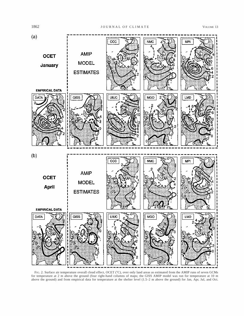
FIG. 2. Surface air temperature overall cloud effect, OCET (8C), over only land areas as estimated from the AMIP runs of seven GCMsfor temperature at 2 m above the ground (four right-hand columns of maps; the GISS AMIP model was run for temperature at 10 mabove the ground) and from empirical data for temperature at the shelter level (1.5–2 m above the ground) for Jan, Apr, Jul, and Oct.


FIG. 2. (Continued ) Clear-sky day is defined as a period when total cloudiness was less than 0.15.


4. Sensitivity of the surface temperature andhumidity fields to the presence of clouds

a. Surface air temperature in the presence of clouds

In Fig. 2, we compare the January, April, July, andOctober OEs of the presence of clouds on near-surfaceair temperature. In empirical data, OCET shows its ob-vious seasonality. In the Northern Hemisphere winter,OCET is positive, while in summer, the effect is op-posite and cooling is associated with the presence ofclouds.6 In the transitional seasons (April and October),in high latitudes, the surface temperature difference be-tween average and clear sky conditions is positive, whileover some midlatitudes and subtropical regions, the dif-ference is negative. The magnitude of the overall effectof cloudiness on surface temperature has a circumpolarpattern. In general, the magnitude of surface temperaturevariation associated with cloud cover is larger in highlatitudes than in low latitudes. Below, we compare, sea-son by season, the OCET estimates between the obser-vations and the GCMs over the NEL.

1) JANUARY

The mean daily OCET in January is warming; thatis, clouds are associated with higher temperatures. Themost prominent OCET is in high latitudes: a 4–8 Kdifference between average and clear sky conditions.All seven GCM AMIP runs tested reproduced the signand the pattern of the winter OCET. Four GCMs (UIUC,MPI, CCC, and NMC) are able to correctly reproducethe magnitude of the OCET. The least accurate OCETreproductions are in the GISS and LMD AMIP runs. Inthese runs, the OCET in high latitudes varies in the rangeof 0–4 K and is underestimated by a factor of 2 or more.A negative OCET over east Siberia, which is seen inthe GISS and LMD OCET estimates, is not supportedby empirical data.

2) APRIL

The mean daily temperature difference in high lati-tudes in the empirical data still remains positive, whilethe magnitude is smaller than that in January. In certainmidlatitudes and subtropical regions, the temperaturedifference turns out to be negative. The UIUC, MGO,LMD, and MPI models properly reproduce the abovepattern, but the magnitude over the polar region in theUIUC and MPI models is higher than that in empiricaldata by 2–4 K. In the MGO model, the cooling asso-

6 Groisman et al. (1996) show that in the summer, the cloud effectsover most of NEL have distinctive patterns and different signs indaytime and nighttime (cf. Fig. 3 in Groisman et al. 1996). Therefore,mean daily cloud effects in summer, which we are comparing now,are an algebraic sum of the strong patterns, which are quite differentduring the diurnal cycle.

ciated with cloud cover is disproportionately amplifiedover Asia. The CCC and NMC models basically repro-duce the same pattern of temperature difference in highlatitudes as in the observations, but they do not repro-duce the cooling associated with cloudiness over somemidlatitudes and subtropical regions. This peculiarity ofthe OCET pattern in these two GCMs becomes morevisible in the summer season and will be discussed indetail in the next paragraph. In contrast, the high-latitudewarming with cloud cover is not properly reproducedin the GISS model, where the OCET over the east Arcticregion is negative.

3) JULY

The mean daily OCET in summer is cooling. Theaverage climate is associated with a July temperaturethat is 1–2 K lower than clear sky conditions. As men-tioned above, this is a manifestation of the daytimecloud effects (Groisman et al. 1996). Four AMIP runs(UIUC, GISS, LMD, and MGO) properly reproduce thesign, pattern, and magnitude of the July OCET. The MPIAMIP run reproduces the pattern and sign but showssome positive bias in OCET. In this run, the averageclimate is associated with temperatures 0–1 K lowerthan clear sky conditions.

The comparison of our empirical estimates of theOCET with two other AMIP runs (CCC and NMC) gavedisturbing results. The sign of the July OCET in thesetwo GCM AMIP runs is opposite to that observed. Toclarify the consequences of these differences, let us as-sume a climate sensitivity experiment (2 3 CO2, aerosolor solar forcing) or a paleoclimatic reconstruction thatmight use these models. In new (and unknown) climateconditions, the cloud cover can change in any direction,and many of the modern climate sensitivity experimentshave shown a significant contribution of these changesto the results of such experiments (IntergovernmentalPanel on Climate Change 1990, 1996). A wrong OCETsign then will produce an unpredictable bias in mete-orological elements, surface air temperature, and cloud-iness, thus affecting all changes in surface climatologyassociated with the forcing under investigation (or thepaleoclimatic reconstruction). We are not able to foreseethese unpredictable changes, but we can state that in thecurrent climate (and the AMIP simulations forced bycontemporary sea surface variations), the present ver-sions of these two GCMs reveal strong contradictionswith the observed climate. These contradictions shouldbe fixed before these versions of the GCMs can be fur-ther used in any climate change assessments.

The mean daily OCET is an algebraic sum of hourlyOCET, and these effects have opposite signs in day andnight (Groisman et al. 1996). For the CCC and UIUCAMIP runs, we were able to expand our analyses of thesummer OCET to assess day–night differences in theOCET. Figure 3 shows the afternoon and nighttimeOCETs that were derived from these model AMIP runs


FIG. 3. Jul OCET (8C) estimated over only land areas from the CCC and UIUC AMIP model runs and from empirical data: (a) localafternoon OCET and (b) nighttime OCET. Clear-sky and overcast days are defined as periods when total cloudiness was less than 0.15 andgreater than 0.85, correspondingly.

and empirical estimates. It is clear that the major prob-lem revealed in Fig. 2 for summer OCET in the CCCmodel is in the daytime. Recent studies (Stuart and Isaac1994; Isaac and Stuart 1996) specifically address theproblems of the CCC model, especially the relationshipbetween precipitation from cumulonimbus and toweringcumulus and temperature in the Mackenzie River Valley.They explain the contradiction between observationsand the model output as follows: ‘‘the model overpre-dicts the occurrence of convective clouds and under-estimates the occurrence of stratiform clouds.’’ Ouranalysis locates the season (summer), area (entire north-ern extratropical land area), and time of day (daytime)when the CCC model is out of range with observations.This strongly supports the hypothesis of Isaac and Stuart(1996) that something is wrong with the convectivescheme of the CCC model under investigation.

The comparisons of July afternoon and nighttime

OCETs derived from the UIUC model with those de-rived from empirical data suggest that this model prop-erly reproduces the afternoon cooling associated withcloudiness, although the magnitude of this cooling is1–2 K lower than that in the empirical data. Unfortu-nately, the nighttime warming associated with cloudsover the midlatitude regions is not shown in the AMIPrun of the UIUC model. The mean daily OCET in theUIUC model is among the best in terms of its corre-spondence with the empirical data. But the amplitudeof the OCET diurnal cycle in this model is much lessthan that in the observed OCET.

We were not able to assess in more detail the problemswith the summer NMC OCET because we had onlymean daily values from this AMIP run. However, a re-cent analysis by Higgins et al. (1996) indicates that theNMC GCM overestimates convective afternoon precip-itation (at least over the Mississippi River Basin). This


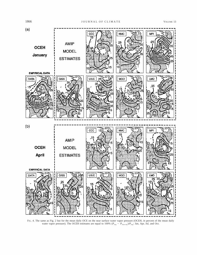
FIG. 4. The same as Fig. 2 but for the mean daily OCE on the near surface water vapor pressure (OCEH, in percent of the mean dailywater vapor pressure). The OCEH estimates are equal to 100% (Pavg 2 Pclear sky)/Pavg: Jan, Apr, Jul, and Oct.


FIG. 4. (Continued )


suggests that the model generates many more cumulusclouds than are necessary in conjunction with the warm-er-than-necessary surface. These two factors may leadto ‘‘a warm surface—lots of clouds’’ association in theNMC AMIP runs output that contradicts empirical data.

4) OCTOBER

The UIUC and MPI models correctly reproduce theempirical OCET map, with the maximum warming overpolar regions near 1008E and cooling over subtropicalregions of North America and Eurasia. The GISS, NMC,and CCC models can basically produce the OCET pat-tern in empirical data, but the maximum warming centernear 1008E in high latitudes doesn’t appear on the mapsderived from these models. In addition, the subtropicalnegative OCET is not reproduced in the CCC and NMCmodels. In the MGO and LMD models, the distributionof the surface air differences with cloud cover is similarto that in the observations except over east Asia, wherethese models produce negative OCET, which is oppositeto the empirical data.

5) CONCLUSION

In conclusion, there is a general agreement in repro-ducing the associations between cloudiness and surfacetemperature in the cold season among all models tested.The largest intermodel difference in the OCET occurredin July. In comparison with the other six AMIP runs,the UIUC run is the most effective in producing themean daily OCET. We were able to compare the diurnalcycle of the OCET with empirical data for only twoGCMs—CCC and UIUC. One of these models, UIUC,performs much better than the other GCM and showsa proper sign and pattern of the mean daily OCET and,what is especially important, the afternoon OCET. How-ever, the UIUC model does not produce the midlatitudenighttime warming associated with cloud cover. Thus,we can conclude that for modern climate modeling, aproper reproduction of the OCET for the diurnal vari-ation of the surface air temperature is still a major chal-lenge.

b. Near-surface humidity fields in the presence ofclouds

There is a difference in characteristics that were se-lected by different model groups to represent the near-surface humidity field in their AMIP runs. Four GCMs(GISS, NMC, LMD, and CCC) provide informationabout specific humidity, the UIUC model output pro-vides absolute humidity, the MGO model output pro-vides water vapor pressure, and the MPI model outputcontains dewpoint temperatures at the shelter level.7 The

7 For the GISS AMIP run, we have specific humidity data at thefirst model level, that is, approximately 200 m above the ground.

humidity characteristic that we selected for our inter-comparison from empirical data is water vapor pressure.In Fig. 4, we present its mean daily changes in thepresence of cloud cover in percent of average watervapor pressure.8 For the purpose of comparability, weuse the percentage of the variation of water vapor pres-sure between average and clear-sky conditions to presentour OCEH estimates. Therefore, when the average watervapor pressure in the GCM deviates from its observedvalues, these deviations also contribute to the OCEHestimates shown in Fig. 4.

Empirical data show that the OCEH is positive in allfour seasons (except for the Arctic and wet and cloudyNorth Pacific coastal areas), indicating that clear-skyconditions are usually associated with less-than-averageatmospheric water vapor. In winter, the overall magni-tude of this relative change in the Northern Hemisphereis larger than in summer. Below we compare, season byseason, the OCEH estimates between the observationsand the GCMs over the NEL.

1) JANUARY

In the empirical observations, the relative change ofwater vapor pressure increases with latitude, reaching45% or more over the northeastern tip of North America,the Arctic region, and central Siberia. This phenomenonis related to the decrease of water vapor content in theatmosphere from low to high latitudes. The UIUC, MPI,NMC, CCC, LMD, and MGO models basically repro-duce this water vapor change pattern. But there is apositive bias (15%–30%) in the MPI model in high lat-itudes and a negative bias (10%) in the CCC model.Over the entire Northern Hemisphere, the MGO andLMD models reproduce the OCE with a 10% negativebias, as compared to the empirical data. The GISS modelcannot properly reproduce the observed water vaporchange distribution. There even exists a negative dif-ference of water vapor pressure between average andclear-sky conditions over the polar region near 1408Ein the OCEH, which was reproduced by this model.

2) APRIL

In April, the OCEH magnitude (in percent) is smallerthan in January, but the whole OCEH pattern in NEL

8 For the CCC AMIP run, we evaluate the OCEH for each hourand then construct its daily average value. For other GCMs and forempirical data, we used method two of the calculations (see appendixA). For the MPI AMIP run, the 12-h mean values of dewpoint tem-perature were converted to water vapor pressure values using theMagnus formula beforehand. We checked the effect of such a con-version (when applied to empirical data) and found its contributionto our estimates to be negligible. This indicates that it does not matterwhich humidity characteristic was used for the estimates shown inFig. 4. Therefore, a higher sensitivity of the near-surface humidityfield to cloud cover that was revealed for the MPI AMIP output isnot a product of a different mean 12-h averaged characteristic ofhumidity in the model output.


is similar in these two months. The OCEH patterns de-rived from the UIUC, MPI, CCC, NMC, and MGO mod-els are roughly in line with the observed patterns. Still,the MPI model overestimates the OCEH magnitude inhigh latitudes, the NMC and CCC models underestimatethe OCEH value by about 10% in midlatitudes, and thereis a 10% negative bias in the OCEH derived from theMGO model over land areas of the Northern Hemi-sphere. In the GISS model over the Arctic, the differ-ences in water vapor pressure are the smallest, whichis opposite of that in the empirical data.

3) JULY

The summer pattern of the OCEH is totally differentfrom other seasons. The maximum water vapor pressuredifference under average and clear-sky conditions oc-curs over the Tibetan Plateau and the Rocky Mountainregion of North America instead of the polar regions(as in winter, spring, and autumn). Although the absolutevalues of the summer OCEH are the greatest, their mag-nitude in percent is the smallest and the value of themaximum-value contour line is only 15%. There arelarger differences in reproducing the empirical OCEHamong the models under consideration. The UIUC,NMC, and MGO models are the only ones that canreproduce the whole pattern in the empirical observa-tions, including the maximum water vapor pressure cen-ters, but the magnitude of the OCEH reproduced by theUIUC model over these regions is 5% less than ob-served. There are significant biases over polar regionsin the estimates derived from the GISS and NMC mod-els. In both these models, over most of the polar regions,the water vapor pressure difference (in percent) is largerthan in the observations, especially in the GISS model,where the difference compared with observations canreach about 20%. In the CCC model, the pattern of theOCE on surface humidity is almost opposite to that inthe empirical data, and in this model, the strongestOCEH still remains over high latitudes. Noticeably, inall seven models, there is the same maximum in theOCEH over the Tibetan Plateau and Rocky Mountainsas in the observations.

For this midsummer month, we also analyzed theoverall effect of cloudiness on diurnal variations of sur-face humidity in empirical data and in the CCC andUIUC models (not shown). In general, the OCEH pat-tern estimated from the observations in afternoons issimilar to that at nighttime. Both patterns are similar tothe above-mentioned mean daily pattern. The differencein the OCEH between afternoon and nighttime is thatthe magnitude of the afternoon OCEH is larger than atnighttime by about 5%–10%. The diurnal variation ofthe OCEH in the UIUC model is the same as that inthe empirical data, but in the CCC model, the diurnalvariation of the OCEH observed in the empirical datais not reproduced.

4) OCTOBER

The pattern of the OCEH in empirical observationsis similar to that in April. The UIUC, MPI, NMC, CCC,and MGO models fundamentally reproduce this pattern,but the MPI model overestimates the value over polarregions by about 10% and the MGO and CCC modelsunderestimate the value by about 10% over most areasof the Northern Hemisphere. The GISS model cannotcorrectly reproduce the pattern of the autumn OCEH.

5) CONCLUSION

Many studies have verified that water vapor in theatmosphere has a positive greenhouse effect. That is,much more water vapor content can cause an increasein surface temperature, and vice versa. However, therelationship between the variations of surface water va-por pressure and surface air temperature associated withcloudiness seems complicated. In winter, an increase insurface water vapor is associated with cloud cover (Fig.4) and corresponds to a warmer surface (Fig. 2). How-ever, in summer, the same figures show that an increasein water vapor pressure associated with cloud cover isrelated to cooling at the surface. This situation also ex-ists in the diurnal variation of water vapor pressure. Thephysical processes involving cloudiness–water vapor–surface temperature interaction need further investiga-tion. These processes are most visible in the Tropics,and therefore the assessment of tropical OCET andOCEH is singled out in the next section.

5. Surface air temperature and humidity in theTropics in the presence of clouds

The accumulation of synoptic data from the Tropicsgives us an opportunity to make a pilot analysis of theeffects of the presence of clouds in the tropical atmo-sphere on the near-surface meteorological fields. Thestandard approach that we applied to the extratropicalatmosphere in the previous sections does not work wellin the Tropics because we were not able to accumulatethe necessary amount of clear-sky meteorological eventsin the daytime anywhere in the humid Tropics. We stilluse the clear-sky observations to characterize the night-time effects of clouds, but only as an additional tool tocheck our results for nighttime cloud effects. For thedaytime, we have to use a different statistic to describecloud effect, and so we selected OCE1 (the differencebetween the values of the meteorological element, f,under average and overcast climate conditions). We usedOCE1 throughout this section for both daytime andnighttime, and we verified our results/conclusions forthe nighttime cloud effects using OCE. This allowed usto proceed with an assessment of the mean daily OCE1

from all seven GCMs in the wet Tropics. In the tropicalregions, cloud diurnal variations dominate in the widerange of timescales exhibited by clouds and influence


TABLE 1. Specific humidity, q (g kg21), and overall cloud effect on surface air temperature, OCET1 (K), in tropical regions.

Stations

Jan

q OCET1

Apr

q OCET1

Jul

q OCET1

Oct

q OCET1

AfternoonCentral and western PacificSoutheast Asia (north of the equator)South AsiaCentral and South AmericaAfrica, SahelThe Hawaiian IslandsMountains

944237249

410

17131315

513

8

20.521.421.421.121.321.322.2

18171716

813

9

20.621.521.520.920.920.921.3

19191917161413

20.621.021.020.821.420.721.0

191717171215

9

20.621.421.421.021.520.921.5

NighttimeCentral and western PacificSoutheast Asia (north of the equator)South AsiaCentral and South AmericaAfrica, SahelThe Hawaiian IslandsMountains

17111414

512

8

20.10.30.60.20.60.90.9

17151615

91210

20.120.420.4

0.20.50.30.3

18191817161413

20.120.320.320.120.5

0.10.1

181616161414

20.120.1

0.420.0

0.20.3

N/A

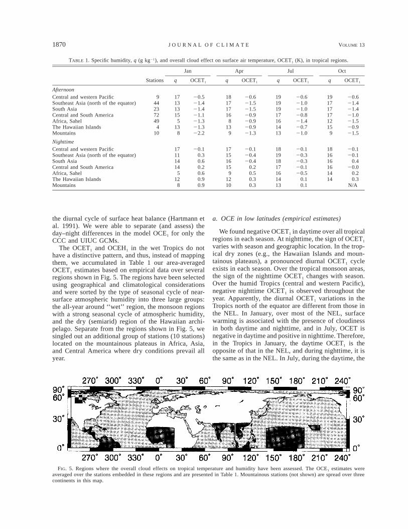
FIG. 5. Regions where the overall cloud effects on tropical temperature and humidity have been assessed. The OCE1 estimates wereaveraged over the stations embedded in these regions and are presented in Table 1. Mountainous stations (not shown) are spread over threecontinents in this map.

the diurnal cycle of surface heat balance (Hartmann etal. 1991). We were able to separate (and assess) theday–night differences in the model OCE1 for only theCCC and UIUC GCMs.

The OCET1 and OCEH1 in the wet Tropics do nothave a distinctive pattern, and thus, instead of mappingthem, we accumulated in Table 1 our area-averagedOCET1 estimates based on empirical data over severalregions shown in Fig. 5. The regions have been selectedusing geographical and climatological considerationsand were sorted by the type of seasonal cycle of near-surface atmospheric humidity into three large groups:the all-year around ‘‘wet’’ region, the monsoon regionswith a strong seasonal cycle of atmospheric humidity,and the dry (semiarid) region of the Hawaiian archi-pelago. Separate from the regions shown in Fig. 5, wesingled out an additional group of stations (10 stations)located on the mountainous plateaus in Africa, Asia,and Central America where dry conditions prevail allyear.

a. OCE in low latitudes (empirical estimates)

We found negative OCET1 in daytime over all tropicalregions in each season. At nighttime, the sign of OCET1

varies with season and geographic location. In the trop-ical dry zones (e.g., the Hawaiian Islands and moun-tainous plateaus), a pronounced diurnal OCET1 cycleexists in each season. Over the tropical monsoon areas,the sign of the nighttime OCET1 changes with season.Over the humid Tropics (central and western Pacific),negative nighttime OCET1 is observed throughout theyear. Apparently, the diurnal OCET1 variations in theTropics north of the equator are different from those inthe NEL. In January, over most of the NEL, surfacewarming is associated with the presence of cloudinessin both daytime and nighttime, and in July, OCET isnegative in daytime and positive in nighttime. Therefore,in the Tropics in January, the daytime OCET1 is theopposite of that in the NEL, and during nighttime, it isthe same as in the NEL. In July, during the daytime, the


FIG. 6. Nighttime overall cloud effect on the July surface air tem-perature (OCET and OCET1) in the Northern Hemisphere south of608N (8C) vs surface air specific humidity q (g kg21). Empiricalestimates at each location (totally approximately 1000 sites) havebeen sorted by q and smoothed by a 20-point running average pro-cedure.

negative sign of OCET1 is maintained throughout alllatitudes, while during the nighttime in the Tropics, dif-ferent regions have different OCET1 signs.

OCEH1 (not shown) does not vary dramatically overthe Tropics in the diurnal cycle. The water vapor pres-sure in the Tropics is much larger than that in the ex-tratropical regions; therefore, the percentage of watervapor pressure variations associated with cloudiness aresmaller than in the midlatitudes or high latitudes (vary-ing by absolute value from 5%–15%). Among the newfeatures that were not observed in the NEL, we en-countered negative OCEH1 in both April and July oversoutheast Asia. In short, the association of cloudinesswith surface humidity generally is the same betweenextratropical and tropical regions.

b. OCE in Tropics in the GCM AMIP runs

At present, of the seven AMIP GCM runs, only theUIUC and CCC models provide us with 6-hourly out-puts, and the output from the UIUC model is only forJuly. The specifics of the OCE in tropical regions aremostly in the diurnal cycle in the warm/wet season.Therefore, in this section, we focus on comparisons be-tween daytime and nighttime empirical OCET1 andOCEH1 estimates and those derived from the UIUC andCCC GCMs during the midsummer month of the North-ern Hemisphere—July. Because the model grid reso-lution cannot cover small islands, four continental re-gions shown in Fig. 5, southeast Asia, south Asia, westAfrica, and Central and South America, are selected forcomparison with the observations.

In the UIUC model, the diurnal cycle of the OCETis simulated quite well, reproducing the negative OCET1

over these four monsoon regions in both daytime andnighttime. The simulated OCEH1 in the UIUC model isnot in full agreement with the observations. At night-time, it is positive over all four regions, but in the em-pirical data, this happens only over south Asia and trop-ical regions of America. In daytime, in the UIUC model,the OCEH1 over Central and South America is negative,which contradicts the empirical OCEH1 estimates. Overthree other monsoon regions, the signs of empirical andUIUC daytime OCEH1 coincide.

In the CCC model, the daytime OCET1 in the tropicsis in agreement, while the nighttime OCET1 is almostopposite to the observations. In that model, only oversouth Asia is there a slightly negative temperature dif-ference between overcast and average situations, whichis in line with empirical estimates (also see Fig. 3). Thesimulated OCEH1 in the CCC model is basically inagreement with observations, except that the magnitudeof the OCEH1 in the CCC model is smaller than that inthe empirical estimates.

6. Water vapor and the nighttime OCETIn this section, the OCET specifically refers to the

nighttime. Over the NEL, the nighttime OCET remains

positive and declines with the decrease of geographiclatitude and with the change from winter to summer (insummer in polar regions, the nighttime OCET is neg-ative due to the polar day phenomenon). Over the Trop-ics in winter, the nighttime OCET is positive over alltropical regions except the western and central Pacific,but in summer over monsoon regions and in the per-manent convection zone of the central and western Pa-cific, the OCET becomes negative, while over dry trop-ical regions it remains positive.

Sun and Groisman (1998) examined the associationbetween near-surface humidity and the nighttime OCETsouth of 608N in each season. These results (only forsummer season) are shown in Fig. 6 for the empiricalestimates of nighttime OCET and in Fig. 7 for the es-timates derived from the UIUC and CCC AMIP runs.In those figures, the abscissa represents the surface spe-cific humidity q (g kg21) and the ordinate shows theOCET/OCET1 estimates (K). We also constructed globalmaps of surface-specific humidity in order to locate the


FIG. 7. Nighttime overall cloud effect on the Jul surface air tem-perature (OCET1) in the Northern Hemisphere south of 608N (8C)versus surface air specific humidity q (g kg21). Estimates are basedon the AMIP runs with UIUC and CCC global climate models (land-only grid cells are used to make it comparable with Fig. 6).

geographic position of the point on the functional curvebetween the OCET and surface water vapor. We foundthat in each season, the OCET significantly depends onq, and the relationship between them is nearly linear.

Figure 6 shows the empirical OCET and OCET1 es-timates for July at night. Hourly data of approximately1000 stations qualified for use in constructing this fig-ure. Initially, we calculated the point OCET and OCET1

estimates. They were considered valid point estimateswhen we were able to find at least 30 clear-sky (overcast)cases in the station’s record. Then, these point estimateswere sorted by specific humidity and smoothed by a 20-point running average process. This figure shows animportant (and previously unreported) property of thenight tropical atmosphere that can affect our understand-ing of the self-regulatory mechanisms of climate vari-ations and, specifically, the bounds for projected green-house warming. Regression analysis of the unsmootheddata shown in Fig. 6 gives

2OCET 5 1.25 2 0.07q (R 5 0.09) and (7)2OCET 5 1.4 2 0.10q (R 5 0.26). (8)1

The regressions above show that the nighttime OCETis closely correlated to the surface water vapor, which,in a significant way, determines its geographical andseasonal variations. With the increase of surface watervapor, the nighttime warming associated with clouds islinearly reduced and even reversed to cooling when thesurface-specific humidity surpasses a certain value(about 15.5 g kg21).

Satellite measurements show that warmer tropicaloceans as a whole are associated with a reduced long-wave warming cloud effect (Zhang et al. 1996). Thisconclusion is the same as ours, although Zhang et al.(1996) used sea surface temperature instead of humidityto assess the relationship of cloud cover and the radiativebudget at the top of the atmosphere in the Tropics.9 Inlow latitudes, the atmosphere contains much more watervapor, which absorbs some longwave radiation that isdirected from the surface and from cloud cover. Thus,the exchange between clouds and the surface becomesweaker and affects OCET. Stephens et al. (1994) showedhow the difference between clear and cloudy sky long-wave fluxes to the surface decreases with the increasein integrated water vapor content in the atmosphere.This difference becomes zero when the precipitable wa-ter content in the atmosphere comes close to 50 mm.Thus, the surface is no longer affected by longwaveradiation changes due to the cloud presence. Our resultsalso show that the longwave radiation surface air warm-ing due to the presence of cloud cover is greatly influ-enced by the moisture state of the atmosphere, whichnullifies the radiation effects of cloudiness in the night-time humid tropical atmosphere.

Figure 7 shows the nighttime estimates of the JulyOCET1 based on the UIUC and CCC AMIP runs. Abrief comparison with empirical estimates shown in Fig.6 reveals two major shortcomings. The CCC model pro-vides positively biased OCET1 estimates that never crossthe zero line with an increase of specific humidity. TheUIUC model qualitatively resembles the empirical es-timates, but the threshold, when the negative OCET1

values in this model first appear, is shifted too muchtowards lower values.

9 We also analyzed the relationship between the OCET1 and surfacetemperature and found that the statistical relationship is basicallysimilar to that between the OCET1 and specific humidity but is lesssignificant than the latter. When both humidity and surface temper-ature were included in the regression equation for OCET1 as inde-pendent variables, we did not find any improvement because of themulticollinearity problem: absolute values of near-surface humidityand temperature are closely correlated over most of the globe, es-pecially in humid areas.


7. Summary and conclusions

R Statistics that characterize surface air temperature(OCET) and humidity (OCEH) interactions with cloudcover have been constructed and compared with sim-ilar statistics evaluated from the output of AMIP runsof seven GCMs. Not all GCMs reproduce these in-teractions properly.

R There is a general agreement in reproducing OCETin the cold season among all models tested, but largediscrepancies between empirical data and some mod-els were found for summer conditions.

R The relationship between variations of surface watervapor pressure and surface air temperature associatedwith cloudiness is complex. In winter, an increase insurface water vapor is associated with cloud coverand corresponds to a warmer surface. However, insummer, an increase in water vapor pressure associ-ated with cloud cover is related to cooling at the sur-face.

R The OCET in daytime over all tropical regions is neg-ative in each season. At nighttime, the sign of OCETvaries with season and geographic location. Duringnighttime, the OCET decreases from winter to sum-mer over monsoon regions and remains negativethroughout all seasons over the humid tropical PacificIslands.

R Over the NEL, the nighttime OCET remains positiveand declines with the decrease of geographic latitudeand with the change from winter to summer (in sum-mer in polar regions, the nighttime OCET is negativebecause of the polar day phenomenon). Over the Trop-ics in winter, the nighttime OCET is positive over alltropical regions (except the western and central Pa-cific), but in summer, over monsoon regions and inareas of permanent convection, the OCET becomesnegative, while over dry tropical regions, it remainspositive.

R Internally inconsistent model parameterizations (i.e.,those that do not reproduce present-day relationshipsbetween climatic variables) may mislead users whenapplied beyond the ‘‘control’’ environment of thecurrent climate; that is, when applied to climate-change studies. Therefore, a careful testing of theserelationships to resolve the problems may lead tomore robust models and, thus, will increase the abil-ity of the GCMs to serve as a reliable tool for climatechange studies.

The presented comparison of the GCM AMIP runsand empirical data has been gradually conducted duringthe past four years and characterizes the state-of-the-artof these GCMs at the time of the AMIP runs. The results(especially problems revealed during this comparison)have been conveyed to the model groups. Currently,some of these groups have significantly modified/im-proved their models (particularly MPI, CCC, and UIUC)and/or the cloud cover parameterization (particularly

GISS and CCC), and some of the revealed problems aretherefore historical at this point in time. We stronglyhope that this is the case with the most significant prob-lem revealed during the current study: a wrong sign ofsummer OCET in the CCC GCM. This problem wasreported three years ago to the CCC model group, andnow a new version of this GCM has been released thattook into account the diagnostics shown in Fig. 3 (Fran-cis Zwiers 1998, personal communication).

Acknowledgments. We gratefully acknowledge the co-operation of the National Weather Services of the UnitedStates, Russian Federation, People’s Republic of China,Norway, Sweden, Iceland, Finland, the Netherlands,France, Ireland, United Kingdom, Germany, Poland,Slovakia, Austria, and Romania for providing the datafor this research. Canadian data were furnished to theU.S. National Climatic Data Center by the AtmosphericEnvironment Service of Canada. We also thank AMIPmembers from the Canadian Climate Centre; the Uni-versity of Illinois at Urbana-Champaign, USA; the U.S.National Meteorological Center; the Main GeophysicalObservatory, Russia; the Max Planck Institute, Ger-many; the Laboratoire de Meteorologie Dynamique,France; and the Goddard Institute for Space Studies,USA, as well as Frank Keimig (UMass) for technicalassistance. This work was supported by Grants fromNOAA (NAGP0414), NSF (9501320), and DOE(98A0132).

APPENDIX A

Different Methods to Assess OCE in the Data andTheir Accuracy

Two different computational schemes

From empirical data, Groisman et al. (1996) were ableto evaluate associations of cloud cover with ground sur-face air temperature and humidity characteristics (ab-solute and relative humidity) for each given hour. Then,to obtain a mean daily OCE, we averaged these esti-mates over the 24-h period (method 1). Because thenumbers of observations with clear skies varies sub-stantially during the day and night (especially in summermonths) and because we were able to mimic this pro-cedure only when we process the CCC model output,in this paper, we used an alternative approach to evaluatethe OCE on the mean daily meteorological fields (meth-od 2). In this approach we calculated the mean dailyvalues of these fields and cloud cover and then definedthe clear-sky days as the days with mean daily cloud-iness less than 0.15. This last approach is the only onefeasible when only the mean daily values of GCM runsare available (of course, the threshold 0.15 is an arbi-trary value). Therefore, to be able further compare them,we have to calculate similar quantities from the dataand model output. Figures A1 and A2 show a compar-ison of these two methods of calculation of the sensi-


FIG. A1. Comparison of the two empirical estimates of the mean daily OCET (8C): (a) estimates by the first method, in which the OCETestimates were calculated for each hour in the month separately, and then the arithmetic average of the estimates was produced; (b) estimatesby the second method in which mean daily and cloudiness were calculated first, and then the OCET was estimated from these mean dailyvalues, assuming a clear-sky day as a day with cloudiness less than 0.15; (c) standard deviations of the OCET estimates derived by thesecond method.

FIG. A2. The same as Fig. A1 but for the mean daily OCEH (in percent of the mean daily water vapor pressure).

tivity of surface air temperature and water vapor pres-sure to the presence of clouds for four central monthsin each season. In these figures, we use only the datafrom the former Soviet Union and Mongolia. For thecalculations in method 2, standard deviations of theOCET and OCEH are also shown. These figures showthat differences between these two approaches are notcrucial in the further assessment of the sensitivity ofsurface air temperature and absolute humidity fields to

the presence of clouds. The OCET and OCEH patternsin each season are very similar between method 1 andmethod 2, suggesting that there is no significant differ-ence between them in assessing the overall effect ofcloudiness, but there still exist non-negligible differ-ences in their magnitudes due to the different calculationtechniques. Below we summarize these discrepancies.

In winter and in transitional seasons, the positive sur-face air temperature differences between average and


FIG. A3. Comparison of the daytime OCE (first and third rows) and OCE1 (second and fourthrows) for (a) surface air temperature (8C) and (b) surface water vapor pressure (%). When themean cloud cover is far from 0.5, the magnitude of these statistics changes accordingly. Thus, inthe polar region, with the mean cloud cover much higher than 0.5, the OCE is twice as high asOCE1, while in summer, over desert regions of central Asia, the opposite is true, and the absolutevalues of the OCE1 exceed those of OCE.

clear sky conditions in method 2 are larger than in meth-od 1, and over the polar region, the difference betweenthese two methods can reach 2–4 K. In summer, thenegative OCET values produced by method 2 are small-er than in method 1, especially in high latitudes, wherethe difference in magnitude can reach 1–2 K. Therefore,

the cooling associated with cloudiness estimated bymethod 1 is not as strong as in method 2. The aboveshows that OCET estimates produced by method 2 aresystematically biased toward positive values as com-pared with those obtained by method 1. The magnitudeof the OCEH patterns is larger in method 2 than in


TABLE C1. Standard deviations of empirical estimates of overallcloud effect (OCET and OCEH) (differences between average andclear-sky conditions) generalized for North America. (A) Surface airtemperature (K), and (B) water vapor pressure (%).

Zone Jan Apr Jul Oct

A. Surface air temperature (K)188–308N308–408N408–508N508–608N608–708N708–808N

188–808N

0.280.330.610.510.450.31

0.41

0.180.250.430.380.330.30

0.30

0.130.130.180.330.330.36

0.16

0.190.180.280.450.500.69

0.22

B. Water vapor pressure (%)188–308N308–408N408–508N508–608N608–708N708–808N

188–808N

2.32.94.95.35.54.8

3.7

1.62.13.22.72.83.4

2.4

0.690.891.271.981.872.05

1.10

1.41.42.13.33.96.2

1.7

method 1, especially over the polar regions in winter,spring, and autumn, where it can reach 10%–15% ofthe mean absolute humidity values. The reason for thedifference of the OCE between method 1 and method2 is still not clear. The possible cause may be relatedto the different number of clear-sky cases during night-time and daytime. Nevertheless, some conclusions onthe OCE comparison between the empirical data andthe AMIP GCM runs may need correction to some ex-tent when the GCM outputs with the diurnal cycle res-olution are available.

APPENDIX B

The Use of Overcast Instead of Clear-SkyConditions

Following Eq. (1), Groisman et al. (1996) defined theoverall cloud effect—OCE on meteorological elements,f, related to clear-sky conditions (D)—as a differencebetween mean values of this element, E(f ), and its meanvalues under clear-sky conditions only, E(f | y ∈ D).When we expanded our analyses to the humid Tropics,this definition became too restrictive because even in a50-yr-long time series, we often were not able to securea substantial sample size of clear-sky conditions to es-timate E(f | y ∈ D). Therefore, as a supplementary tool,we use modified statistics based on overcast conditions,D1:

OCE1(f | y ∈ D1) 5 E(f | y ∈ D1) 2 E(f ). (B1)

Here, we change the sign in (B1) to make it comparablewith (1). Overcast conditions represent another ‘‘ex-treme’’ in cloud cover. The linearity of the substitutionof (1) by (B1) is not granted, and we expected that thecomparison of climatic conditions when the sky is to-tally obscured by cloud cover with average climatecould reveal new important features of the relationshipbetween f and cloud cover. Generally, this does nothappen. The comparison of OCE and OCE1 for surfaceair temperature and humidity in NEL (e.g., Fig. A3)shows that the patterns of these statistics resemble eachother, and differences in magnitude in some regions canbe easily attributed to the fact that mean cloud cover inthese regions is closer to clear-sky conditions (summerseason in the deserts of central Asia) or to overcastconditions (polar regions). We do not normalize ourOCE and OCE1 estimates by the mean difference be-tween mean cloud cover and clear/overcast conditions.This is not necessary until we can retrieve/compute fromthe GCMs’ output the same quantities as from the ob-servational data. But the use of OCE1 statistics becomesour best bet to properly and empirically assess the cloudeffects on other meteorological elements in the humidTropics, in polar regions with extensive stratiform cloudcover, and in any location where clear-sky conditionsare rare.

APPENDIX C

Accuracy of the Empirical OCET and OCEHEstimates

Standard deviations of empirical estimates of cloudeffects (Figs. A1c and A2c) are quite small and give ageneral idea about the statistical significance of the re-vealed ‘‘overall cloud effects’’ on these fields. For NorthAmerica, these estimates are generalized in Table C1.They are similar to those shown in the figures with theexception of the wet Tropics (188–308N—Florida andCaribbean islands), where the sample size for clear skiesis quite small in summer months, even when we use40–50 yr of observations and lenient definitions of clearskies in method 2. However, we note that the smallnegative values of summer OCET are nevertheless sta-tistically significantly different from zero everywhereover northern Eurasia, and thus, the sign of this effectis well defined. The same is true for most of NorthAmerica, with a prominent exception over the north-eastern coastal regions of the United States and alongthe southern shores of the Great Lakes.

REFERENCES

Abakumova, G. M., E. M. Feigelson, V. Russak, and V. V. Stadnik,1996: Evaluation of long-term changes in radiation, cloudiness,and surface temperature on the territory of the former SovietUnion. J. Climate, 9, 1319–1327.

Arking, A., 1991: The radiative effects of clouds and their impacton climate. Bull. Amer. Meteor. Soc., 72, 795–813.

Cess, R. D., and Coauthors, 1991: Interpretation of snow–climatefeedback as produced by 17 general circulation models. Science,253, 888–892., W. L. Gates, J.-J. Morcrette, and L. Corsetti, 1992a: Comparisonof general circulation models to Earth Radiation Budget Exper-


iment data: Computation of clear-sky fluxes. J. Geophys. Res.,97 (D18), 20 421–20 426., E. F. Harrison, P. Minnis, B. R. Barkstrom, V. Ramanthan, andT. Y. Kwon, 1992b: Interpretation of seasonal cloud–climate in-teractions using Earth Radiation Budget Experiment data. J.Geophys. Res., 97, 7613–7617., and Coauthors, 1993: Uncertainties in CO2 radiative forcing ingeneral circulation models. Science, 262, 1252–1255.

Chanine, M. T., 1995: Observation of local cloud and moisture feed-backs over high ocean and desert surface temperatures. J. Geo-phys. Res., 100 (D5), 8919–8927.

Del Genio, A. D., M.-S. Yao, W. Kovari, and K. K.-W. Lo, 1996: Aprognostic cloud water parameterization for global climate mod-els. J. Climate, 9, 270–304.

Gaffen, D. J., and W. P. Elliott, 1993: Column water vapor contentin clear and cloudy skies. J. Climate, 6, 2278–2287.

Gates, W. L., 1992: AMIP: The Atmospheric Model IntercomparisonProject. Bull. Amer. Meteor. Soc., 73, 1962–1970., and Coauthors, 1999: An overview of the results of the At-mospheric Model Intercomparison Project (AMIP 1). Bull. Amer.Meteor. Soc., 80, 29–55.

GEWEX, 1990: Scientific plan for the Global Energy and Water CycleExperiment. WMO, Geneva, Switzerland, Rep. WCRP-40(WMO/TD 376), 83 pp.

Goody, R., J. Anderson, and G. North, 1998: Testing climate models:An approach. Bull. Amer. Meteor. Soc., 79, 2541–2549.

Groisman, P. Ya., and P. M. Zhai, 1995: Climate variability underclear skies: Applications for the cloud and snow cover feedbackproblems. Proc. Sixth Int. Meeting on Statistical Climatology,Galway, Ireland, University College, All-Ireland Committee onStatistics, Amer. Meteor. Soc., European Union, Irish Meteo-rological Service, and World Meteorological Organization, 605–608., T. R. Karl, and R. W. Knight, 1994a: Observed impact of snowcover on the rise of continental spring temperatures. Science,263, 198–200., , , and G. Stenchikov, 1994b: Changes of snow cover,temperature, and the radiative heat balance over the NorthernHemisphere. J. Climate, 7, 1633–1656., P.-M. Zhai, and E. L. Genikhovich, 1995: Cloud and snowcover effects on the surface–atmosphere interactions. ExtendedAbstracts, Papers Presented at the Joint Meeting of the CanadianGeophysical Union-Hydrology Section (CGU-HS) and Inter-national GEWEX Workshop on Cold-Season/Region Hydrome-teorology, Banff, AB, Canada, GEWEX, 209–212., E. L. Genikhovich, and P. -M. Zhai, 1996: ‘‘Overall’’ cloudand snow cover effects on internal climate variables: The useof clear sky climatology. Bull. Amer. Meteor. Soc., 77, 2055–2065., , R. S. Bradley, and B. M. Ilyin, 1997: Assessing surface–atmosphere interactions from former Soviet Union standard me-teorological data. Part II. Cloud and snow cover effects. J. Cli-mate, 10, 2184–2199.

Hahn, C. J., and S. G. Warren, 1999: Extended edited synoptic cloudreports from ships and land stations over the globe, 1951–1996.Data Set Documentation, NDP 026C, 77 pp. [Available fromCarbon Dioxide Information and Analysis Data Center, OakRidge National Laboratory, Oak Ridge, TN 37831.], , and J. London, 1995: The effect of moonlight on ob-servation of cloud cover at night, and application to cloud cli-matology. J. Climate, 8, 1429–1446.

Harrison, E. F., P. Minnis, B. R. Barkstrom, V. Ramanathan, R. D.Cess, and G. G. Gibson, 1990: Seasonal variation of cloud ra-diative forcing derived from the Earth Radiation Budget Ex-periment. J. Geophys. Res., 95, 18 687–18 703.

Hartmann, D. L., K. J. Kowalewsky, and M. L. Michelsen, 1991:Diurnal variations of outgoing longwave radiation and albedofrom ERBE scanner data. J. Climate, 4, 598–617.

Henderson-Sellers, A., 1992: Continental cloudiness changes thiscentury. GeoJournal, 27.3, 255–262.

Higgins, R. W., K. C. Mo, and S. D. Schubert, 1996: The moisturebudget of the central United States in spring as evaluated in theNCEP/NCAR and the NASA/DAO reanalyses. Mon. Wea. Rev.,124, 939–963.

Intergovernmental Panel on Climate Change (IPCC), 1990: ClimateChange. The IPCC Scientific Assessment. J. T. Houghton et al.,Eds., Cambridge University Press, 362 pp., 1996: Climate Change 1995: The Science of Climate Change.The Second IPCC Scientific Assessment. J. T. Houghton et al.,Eds., Cambridge University Press, 572 pp.

Isaac, G. A., and R. A. Stuart 1996: Relationships between cloudtype and amount, precipitation, and surface temperature in theMackenzie River valley—Beaufort Sea area. J. Climate, 9, 1921–1941.

Kaas, E., and P. Frich, 1995: Diurnal temperature range and cloudcover in the Nordic countries: Observed trends and estimatesfor the future. Atmos. Res., 37, 211–228.

Phillips, T. J., 1994: A summary documentation of the AMIP models.PCMDI Rep. 18, UCRL-ID-116384, 343 pp. [Available fromProgram for Climate Model Diagnosis and Intercomparison, Uni-versity of California, Lawrence Livermore National Laboratory,Livermore, CA 94550.]

Polyak, I. I., 1996: Computational Statistics in Climatology. OxfordUniversity Press, 358 pp.

Potter, G. L., J. M. Slingo, J.-J. Morcrette, and L. Corsetti, 1992:Modeling perspective on cloud radiative forcing. J. Geophys.Res., 97 (D18), 20 507–20 518.

Randall, D. A., and Coauthors, 1994: Analysis of snow cover feed-backs in 14 general circulation models. J. Geophys. Res., 99(D10), 20 757–20 771.

Robock, A., C. A. Schlosser, K. Ya. Vinnikov, N. A. Speranskaya,J. K. Entin, and S. Qiu, 1998: Evaluation of AMIP soil moisturesimulations. Global Planet. Change, 19, 181–208.

Rossow, W. B., and Z.-C. Zhang, 1995: Calculation of surface andtop of atmosphere radiation fluxes from physical quantities basedon ISCCP datasets: Part 2. Validation and first results. J. Geo-phys. Res., 100 (D1), 1167–1197.

Sellers, P. J., and Coauthors, 1996: The ISLSCP Initiative 1 globaldatasets: Surface boundary conditions and atmospheric forcingsfor land–atmosphere studies. Bull. Amer. Meteor. Soc., 77, 1987–2005.

Stephens, G. L., A. Slingo, M. Webb, and I. Wittmeyer, 1994: Ob-servations of the earth’s radiation budget in relation to atmo-spheric hydrology. 4: Atmospheric column radiative coolingover the world’s oceans. J. Geophys. Res., 99, 18 595–18 604.

Stouffer, R. J., S. Manabe, and K. Ya. Vinnikov, 1994: Model as-sessment of the role of natural variability in recent global warm-ing. Nature, 367, 634–636.

Stuart, R. A., and G. A. Isaac, 1994: A comparison of temperature–precipitation relationships from observations and as modeled bythe general circulation model of the Canadian Climate Centre.J. Climate, 7, 277–282.

Sun, B.-M., and P. Ya. Groisman, 1998: Cloud cover interactionwith the near-the-surface land meteorology in the GCMs: Com-parison with empirical data in Tropics and the assessment ofthe diurnal cycle of this interaction. Preprints, Ninth Symp. onGlobal Change Studies, Phoenix, AZ, Amer. Meteor. Soc., 321–322., and , 2000: Cloudiness variations over the former SovietUnion. Int. J. Climatol, in press., , R. S. Bradley, and F. Keimig, 1999: Cloud effects on thenear surface air temperature: Temporal changes. Preprints, 10thSymp. on Global Change Studies, Dallas, TX, Amer. Meteor.Soc., 277–281., , , and , 2000: Temporal changes in the observedrelationship between cloud cover and surface air temperature. J.Climate, in press.

USAFETAC, 1986: DATSAV2 Surface USAFETAC Climatic Da-tabase. User Handbook No. 4, December 1986. USAF Environ-


mental Technical Application Center, Asheville, NC, 6 pp. 1appendices. [Available from National Climatic Data Center, 151Patton Avenue, Asheville, NC 28801.]

Weare, B. C., and I. I. Mokhov, 1995: Evaluation of total cloudinessand its variability in the Atmospheric Model IntercomparisonProject. J. Climate, 8, 2224–2238.

Wielicki, B. A., R. D. Cess, M. D. King, D. A. Randall, and E. F.

Harrison, 1995: Mission to Planet Earth: Role of clouds andradiation in climate. Bull. Amer. Meteor. Soc., 76, 2125–2153.

Yao, M.-S., and A. D. Del Genio, 1999: Effects of cloud parame-terization on the simulation of climate changes in the GISSGCM. J. Climate, 12, 761–779.

Zhang, M. H., R. D. Cess, and S. C. Xie, 1996: Relationship betweencloud radiative forcing and sea surface temperatures over theentire tropical oceans. J. Climate, 9, 1374–1384.

the relationship of cloud cover to near-surface

Documents