University of Arkansas, FayettevilleScholarWorks@UARK

Theses and Dissertations

8-2017

Near Surface Geophysics for LithostratigraphicInterpretation at Pedro, Benton County, ArkansasMatthew David RuggeriUniversity of Arkansas, Fayetteville

Follow this and additional works at: http://scholarworks.uark.edu/etd

Part of the Geology Commons, and the Geophysics and Seismology Commons

This Thesis is brought to you for free and open access by ScholarWorks@UARK. It has been accepted for inclusion in Theses and Dissertations by anauthorized administrator of ScholarWorks@UARK. For more information, please contact scholar@uark.edu, ccmiddle@uark.edu.

Recommended CitationRuggeri, Matthew David, "Near Surface Geophysics for Lithostratigraphic Interpretation at Pedro, Benton County, Arkansas" (2017).Theses and Dissertations. 2415.http://scholarworks.uark.edu/etd/2415

Near Surface Geophysics for Lithostratigraphic Interpretation at Pedro, Benton County,

Arkansas

A thesis submitted in partial fulfillment

of the requirements for the degree of

Master of Science in Geology

by

Matthew Ruggeri

University of Arkansas

Bachelor of Science in Geology, 2013

August 2017

University of Arkansas

This thesis is approved for recommendation to the Graduate Council.

___________________________

Dr. Christopher Liner, Ph.D.

Thesis Director

___________________________

Dr. Walter Manger, Ph.D.

Committee Member

___________________________

Mr. Robert Liner, M.S.

Committee Member

Abstract

The roadcut on highway 412 near Pedro, Benton County, Arkansas (MArkUP site L15),

has been of geological interest since its excavation in the 1980s. The roadcut is located within

the Springfield Plateau and displays formations of Lower Mississippian age. The roadcut

contains three mound-like features believed to be olistoliths. This thesis research work adds

geophysical evidence to the geological exposure at the site. The purpose of this research is to

answer the question of whether near surface seismic methods can be used to extend information

at the Pedro outcrop below the ground surface. Specifically, can the top of the Middle

Ordovician Everton contact be identified?

Seismic experiments were conducted by the University of Arkansas MArkUP team,

investigating parts of the Middle Ordovician through Lower Mississippian succession, using a

48-channel Geode seismograph, sledge hammer source, and seismic acquisition software.

Interpretation of P-wave refraction events estimate that the top of the Middle Ordovician

Everton occurs 69 feet below the natural ground surface from the top of the Pedro outcrop at the

location of the largest mound, or approximately 31 feet below the surface of the base of the

roadcut. Estimation of the Chattanooga-Everton contact involved data acquisition, processing to

reduce noise, first arrival event picking and manual inversion to estimate layer depths and

velocities. Ray Trace modeling confirmed inversion results and local stratigraphy was found to

be consistent. The value of this study demonstrates that shallow seismic data can estimate buried

contacts below outcrops and extend geological knowledge in northwest Arkansas.

Acknowledgements

I thank my advisor Christopher L. Liner, for the suggestion of this project, for his

constant support, patience and encouragement throughout this entire process. He was always

willing to lend his knowledge, offer guidance, and volunteer his time in helping my efforts.

Thank you to my committee members Dr. Walter Manger and Robert Liner for providing

knowledge, suggestions, and their time in the interpretation and production of this manuscript.

Thank you to the entire MArkUP team and the many people that helped with the research

and production of this experiment. Special thanks to current and former Arkansas geoscience

students: Lanre Aboaba, Abram Barker, Bryan Bottoms, John Gist, Forrest McFarlin, Daniel

Moser, Josh Stokes, Kevin Liner, Thomas Liner, John Wohlford, and everyone who has helped

along the way. Thank you to all the friends, colleagues and professors I have had the pleasure of

knowing throughout my time at the University of Arkansas.

Lastly, I would like to thank my family and most of all acknowledge my father and

mother, John and Cynthia Ruggeri. Throughout my entire life, you both have always been there

to lend advice, offer help, provide support, and most importantly love me unconditionally. This

is all possible because of the incredible example you set for me as parents. I appreciate

everything you guys have done for me in my life and all the sacrifices you each have made to

help me become the man I am today.

Table of Contents

1. Introduction ............................................................................................................................. 1

2. Location and Geological Setting ............................................................................................. 3

2.1. Location ............................................................................................................................ 3

2.2. Stratigraphy ...................................................................................................................... 4

2.3. Tectonic History ............................................................................................................... 8

3. Methods ................................................................................................................................. 10

3.1. Geophysical Equipment ................................................................................................. 12

3.2. Survey Design, Python ................................................................................................... 12

3.3. Data Acquisition ............................................................................................................. 13

3.4. Data Analysis ................................................................................................................. 17

3.5. SeismicUnix Processing ................................................................................................. 20

3.6. MathematicaTM Manual Inversion .................................................................................. 23

3.7. Ray Trace Modeling ....................................................................................................... 26

4. Interpretation ......................................................................................................................... 29

4.1. Estimation of Seismic Depth to Everton ........................................................................ 29

4.2. Correlation with Nearby Well Control ........................................................................... 30

4.3. Chattanooga Discussion ................................................................................................. 32

5. Conclusions ........................................................................................................................... 32

6. Future Research ..................................................................................................................... 33

7. References ............................................................................................................................. 34

8. Appendices ............................................................................................................................ 36

8.1. Appendix A: Python code for 2D seismic survey design............................................... 36

8.2. Appendix B: SeismicUnix processing flow ................................................................... 38

8.3. Appendix C: MathematicaTM code for interactive seismic refraction fitting ................. 40

List of Figures

Figure 1: Geologic Map showing study area location .................................................................... 2

Figure 2 : Outcrop photograph of Boone-St. Joe contact ............................................................... 7

Figure 3: Stratigraphic column of study site ................................................................................... 8

Figure 4: Surface Geology Map of study area and nearby wells .................................................. 10

Figure 5: Survey design created with Python survey design program .......................................... 13

Figure 6: 5-Layer model and featured layer formations ............................................................... 16

Figure 7: Wiggle Plot created with acquisition data ..................................................................... 19

Figure 8: Trace Offsets generated from survey acquisition ......................................................... 22

Figure 9: Zoomed in image of Figure 8 Trace Offsets ................................................................. 23

Figure 10A: MathematicaTM generated model of analyzed time and offset picks ....................... 24

Figure 10B: MathematicaTM interactive adjustment for analysis ................................................. 25

Figure 11: Rock velocity variation diagram ................................................................................ 26

Figure 12: Ray trace synthetic overlay ......................................................................................... 28

Figure 13: Cshot generated earth model ....................................................................................... 29

List of Tables

Table 1: Survey acquisition geometry details ............................................................................... 13

Table 2: Selected time and offset picks for analysis of Wiggle Plot ............................................ 20

Table 3: Well control data ............................................................................................................. 30

1

1. Introduction

The Multiscale Arkansas Unconventionals (MArkUp) team, at the University of

Arkansas, conducted near-surface seismic geophysical research at a roadcut exposure near Pedro,

Benton County, Arkansas on the south side of Highway 412. The site is known in the University

of Arkansas Geosciences Department outcrop location guide as L15. The Pedro roadcut, herein

termed L15, exposes three mound-like features excavated by a roadcut in the late 1980s, prior to

completion of the highway. The oldest formations exposed at L15 are the Mississippian Lower

Boone and the St. Joe. The depth to the St. Joe-Chattanooga contact, and the thickness of

underlying Devonian Chattanooga Shale were not accurately known, but are estimated based on

the analysis of near surface seismic data and understanding of local stratigraphy. Figure 1 shows

a geologic map of the L15 study area within the Springfield Plateau.

Previous studies in the area include Liner and Liner (1995), who acquired ground

penetrating radar data on a ledge at L15 and developed a radar image of one of the mounds, and

Chandler (2001), who reported conodont sampling and zonation. Several field trips over the

years have featured L15 as a destination, but never had definitive explanation of the mounds at

this unusual site (McGilvery et al., 2016). It remains a point of debate as to the origin of the three

mound-shaped features.

The process of near-surface seismic involves triggering a source generating elastic waves

that travel through near-surface soil and rock layers as direct, surface, reflection and refraction

waves to be measured by geophones acting as sensors at the surface (Liner, 2016). Processing

and analysis of the data allows thickness and velocity of near surface layers to be estimated. Of

the several wave types generated and measured by this apparatus, this study focuses strictly on P-

wave refraction arrivals that can give information about layer velocity, thickness and depth

2

(Telford et al., 1976). One significant limitation of refraction seismology is that refractions only

develop on surfaces where the seismic velocity increases (Liner, 2016). A velocity drop, or

inversion, such as the St. Joe Limestone - Chattanooga Shale interface is effectively invisible to

refraction seismology. For this reason, my primary objective is mapping the Lower Chattanooga

Figure 1. Geologic map that includes the plateaus and nearby provinces surrounding the Ozark

Dome in the Southern Midcontinent. The red star near the center is the location of the L15 study

site near Pedro, Benton County, Arkansas (Bennison, 1986).

3

Shale contact with the higher velocity Middle Ordovician Everton Dolomite, an interface capable

of generating refractions. The depth and clarity of the experimental results depend strongly on

the power of the source, signal processing, local stratigraphy and ambient noise (Telford et al.,

1976).

The equipment used in data collection were two 24-channel Geonics Geode seismographs

connected to form a 48-channel receiver spread. The source was a sledge hammer with an

attached trigger to begin the recording process and a strike plate. The software used in recording

the data traces is Seismodule Controller.

The benefit of near-surface seismic is that it can be used to estimate formation

thicknesses, formation velocities, and determine information below the foot of an outcrop. In this

study, shallow seismic is used to expand the subsurface knowledge about site L15. In addition,

the geophysical analysis can be compared with nearby wells having similar stratigraphy.

The Lower Mississippian rock formations studied at L15 are equivalent to petroleum

reservoir rocks drilled about 100 miles west of L15, for example in Osage County, Oklahoma

(Friesenhahn, 2010). Information gained from near surface seismic at L15 may add to the

understanding of these deeper reservoir rocks.

2. Location and Geological Setting

2.1. Location

The L15 site is a roadcut along the south side of highway 412 near Pedro, Benton

County, Arkansas. This roadcut was excavated during the initial widening and construction of

the highway in the late 1980s. The field site coordinates are 36.17141° N and 94.38985° W with

an approximate elevation of 1040 feet above mean sea level at the top of the roadcut, where

surveyed. Total exposure length at the site is about 1475 feet trending roughly East-West. Close

4

proximity to highway 412 means significant traffic noise that can interfere with seismic data

quality. The road noise is minimized by (1) vertical stacking (Liner, 2016), (2) timing of source

hammer strikes to coincide with minimum traffic, and (3) post-acquisition processing,

particularly offset stacking (Liner, 2016).

2.2. Stratigraphy

L15 is located within the Springfield Plateau of the Ozark Dome. The stratigraphy of

interest is mostly Lower Mississippian, extending deeper into underlying strata of Devonian and

Middle Ordovician age. The formations visible at the roadcut are the Boone and St. Joe

Formations of the Lower Mississippian. Below the St. Joe Formation, the Devonian Chattanooga

Shale, (while not exposed at L15) can be seen cropping out a short distance to the west of L15

(Haley, 1993) and the Chattanooga is exposed in several places along the nearby Illinois River

banks and bluffs. The next deeper formation, based on local well information and area

stratigraphy should be the Middle Ordovician Everton. Neither the Chattanooga or Everton are

visible at the outcrop, but assumed present in the near subsurface.

The age of the formations from oldest to youngest are: The Middle Ordovician Everton,

the Upper Devonian Chattanooga Shale, the Lower Mississippian St. Joe and succeeding Boone

Formations.

The Middle Ordovician Everton Formation is a shallow marine dolomite. It varies in

lithologic character from location to location and commonly includes layers of dolomite,

sandstone, and limestone. At L15 it is likely to be dolomite, and is called as such in nearby wells.

Fossils are not believed to be commonly found within the formation, which can range from about

300-650 feet thick (Purdue, 1907). Typically, the Everton is succeeded by the Middle Ordovician

St. Peter Sandstone, but near L15 the Upper Everton is overlain by the Chattanooga Shale with

5

an unconformable boundary (Dowell et al., 2005). This relationship is confirmed by shallow well

data near the L15 site, later referenced in Table 3.

Above the Middle Ordovician Everton at L15 is the Upper Devonian Chattanooga Shale

(Dowell et al., 2005). The Chattanooga Shale is thought to be entirely Devonian in Arkansas

(Haynes, 1891). It is a black, fissile, clay shale deposited in a deeper marine setting and in many

places, exhibits prominent joints.

The Chattanooga Shale was deposited on an unconformable boundary at the top of the

Middle Ordovician Everton. It contains very few fossils and is locally abundant with pyrite. The

thickness of the Chattanooga Formation is expected to be less than 50 feet, with (Dowell et al.,

2005) estimating 20-25 feet. Research by Manger (2012) and McNabb (2014) conclude that the

Chattanooga Shale thickness at L15 is most likely on the lower end of that average range due to

the possibility of condensed sedimentation. The formation in some places contains a lower

sandstone member known as the Sylamore Sandstone. In well data near L15, the Sylamore is not

reported and is therefore, not likely to be present in the stratigraphy succession at L15.

The St. Joe Limestone Formation shares an unconformable lower contact with the

Chattanooga Shale. The St. Joe represents a rapid early Mississippian transgression across a

shallow carbonate ramp known as the Burlington Shelf (Shelby, 1986). The St. Joe Formation

was deposited across a broad ramp or shelf, but it wasn’t deposited in place. Rather, it was

transported to a deeper marine setting before being deposited. As a consequence, the formation is

suspected to have undergone condensed sedimentation (Shelby, 1986).

The St. Joe Formation is made up of four members: The Bachelor Shale, the Compton

Limestone, the Northview Shale/Limestone, and the Pierson Limestone (ascending order). The

members in total can be as much as 100 feet thick, and the limestones are known to be great

6

bluff formers, containing very little chert.

Above the St. Joe, sharing a conformable boundary, is the Mississippian Boone

Limestone Formation, composed of fine to coarse grained fossiliferous limestone with

interbedded chert (Branner, 1891). The Boone is subdivided into two members, the Upper Boone

and the Lower Boone. Figure 2 shows the Boone-St. Joe contact at L15 shortly after the site was

excavated. The Lower Boone, like that of the St. Joe, wasn’t deposited in place, but rather

transported to deeper water environments during a time of rapid transgression, maximum

flooding and high stand. The Upper Boone generally represents shallower water deposition than

the Lower Boone, and represents a regressive sequence that ends with the Upper Boone

deposition (Shelby, 1986). Maximum Boone thickness in NW Arkansas is about 350 feet, but the

B. Ezeil-1 well 4.77 miles South-Southwest of L15 suggests Boone thickness in the study area of

approximately 240 feet.

Several formations are absent between the Chattanooga and Everton in this area of the

Ozarks due to a series of unconformities (Dowell et al., 2005). These missing formations are

sporadically present in the Ozarks, except along the Eureka Escarpment. This would be the

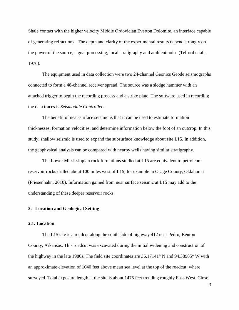
boundary between the Salem and Springfield Plateaus (Manger, 2012). A stratigraphic column in

the vicinity of the L15 outcrop is illustrated as Figure 3.

7

Figure 2. Photograph of the easternmost mound at L15. The red line indicates the location of the

first appearance of bedded chert believed to be the conformable Boone-St. Joe contact (Chandler,

2001).

8

Figure 3. Stratigraphic column representative of the study area. The formations within the

markers indicate those known to exist at L15. Notice that the Lower Devonian, the Silurian, and

the Upper Ordovician are absent (Liner et al., 2013).

2.3. Tectonic History

The early tectonic history of this area was initiated by a cratonic rise of Precambrian

granite to the east. This uplift formed the Ozark Dome, and the present-day St. Francois

Mountains in southeastern Missouri. After this uplift, there was a gentle slope away from the

9

center of the granite dome on which Cambro-Ordovician carbonates were deposited.

Transgressive and regressive seas dominated deposition and erosion from the Paleozoic thru

Mesozoic. Across much of the Ozark Dome, there are widespread unconformities because of

these eustatic cycles (Manger, 2012).

After the deposition of the stratigraphic interval now preserved as the Springfield Plateau,

a series of normal faults cut through those sedimentary formations and even into the deeper

Precambrian basement rocks. These faults trend northeast to southwest with the southeastern side

being the downthrown side. The origin of these faults is uncertain, though one theory assumes

the faults formed due to compressional forces that caused the uplifting of the Ozarks (perhaps the

Ouachita Orogeny) (Dowell et al., 2005). The faulting does not appear to have effected

deposition, since there is no evidence of growth or increased thickness on the hanging wall, and

the faults continue down into the Precambrian basement. A few major faults form escarpments

with up to 1000 feet of displacement on some faults (McCracken, 1971)

The Bella Vista fault is an example of one of the northeast-southwest striking faults that

pass through the study area just west of L15. A splay of the Bella Vista fault splits off to the

north of Pedro, Arkansas, trending in a northeast to southwest pattern almost parallel with the

Bella Vista fault. Both faults are visible in Figure 1. Figure 4 shows a detailed map of the study

area including surface geology and faults. The two faults straddle the town of Pedro, Arkansas,

with the splay on the west and the Bella Vista Fault on the east. The formations and stratigraphy

that lie between the Bella Vista fault and splay are elevated as a horst. The formations visible to

the west of the fault splay and the formations to the east of the Bella Vista fault are the

downthrown sides (Haley, 1993).

L15 lies on the downthrown side of the Bella Vista fault. The horst created by faulting

10

has left the Chattanooga exposed and higher in elevation than adjacent areas to the east and west

of Pedro. This geologic situation acts as a reference for the local Chattanooga thickness, and

explains exposures of the Chattanooga, and why it is not visible at L15.

Figure 4. Google Earth surface geology map of the Pedro Survey site, L15, in northwest

Arkansas. The blue coloring represents Boone Limestone surface exposure and the light green

represents Chattanooga Shale. Local wells used in determining formation depths, as well as the

Bella Vista Fault and splay are denoted by call outs.

3. Methods

The methods used in this research include acquiring shallow seismic at L15 and

constructing cross-sections from nearby wells.

There were two planned and executed shallow seismic surveys for the L15 outcrop. The

first survey was at the base of the outcrop and yielded poor data quality due to road noise and

11

hard rock at the surface making geophone coupling difficult and irregular. Analysis of the first

survey data yielded no useful information on formation depths below the ground surface.

The second seismic survey was shot above the outcrop and centered around the largest,

easternmost mound. For safety and access to good soil coupling, the line was shot approximately

30 feet behind the rock face, parallel to highway 412. The surveys were designed to capture

refraction arrivals to estimate layer velocities and depths. An Excel file list was built that

specified location of each geophone and shot. This thesis reports the results of the second survey

made above the L15 outcrop.

The goal of our analysis is to estimate the depth below the base of outcrop to the top of

the Middle Ordovician Everton Formation. Seismic analysis was augmented by local well

information and stratigraphic formation tops to estimate formation thicknesses and determine

Everton depth at the Pedro site. Surface topography between wells and the Pedro site was

considered using Google Earth elevation profiles to evaluate the well data accuracy with respect

to stratigraphic and near surface seismic findings.

The following is a simplified breakdown of the steps that were taken in determining the

depth to the Chattanooga-Everton formational contact: A survey was initially designed with

Python prior to data acquisition. Geophysical equipment was transported and set up according to

the survey design at L15 and data acquisition was achieved with the use of the Seismodule

Controller program. After the data were acquired, they were processed using SeismicUnix and

became available for modeling. First breaks from the processed data were displayed and modeled

with MathematicaTM. Lastly, SeismicUnix processed data were selected and coded into cshot to

create ray trace model data.

12

3.1. Geophysical Equipment

The equipment necessary for the survey were provided by Dr. Liner and the University of

Arkansas Geosciences Department. The equipment used for each survey included the following:

• 2 Geonics Geode 24-channel seismographs

• 48 single component geophones

• Two 24-takeout spread cables for geophone connection

• Battery with power cable clamps

• Sledge hammer with trigger attached, and metal strike plate

• Laptop with seismic control software for acquisition

• Flags, measuring tape, GPS, compass, field notebook and pencil

3.2. Survey Design, Python

The survey was initially designed using python code to display the source locations,

geophone locations, midpoints and offsets. The survey was designed for refraction seismic

interpretation (Telford et al., 1976), with near offset of 2 feet, far offset of 376 feet, shot interval

of 8 feet, and receiver interval of 2 feet. The near offset distance represents the closest distance

from a shot to a geophone and the far offset represents the furthest distance from a shot to the

last geophone in the array. No geophone array was used, only a single geophone at each receiver

location. All offsets beyond 240 feet were too noisy for interpretation. Figure 5 illustrates the

survey design created with the Python survey design program.

The geological layering at L15 was represented by a 5-layer model as described by

Heiland (1946) and Telford et al. (1976). This model assumes no dip, plane interfaces and no

topography. All these are reasonable assumptions at the survey location with the 240 feet

13

Figure 5. Survey design created with the Python survey design program. Red dots indicate where

the shot locations were and the blue dots, located relatively in the center, represent the 48

geophones.

maximum usable offset.

Geometry details from the Python survey design program are shown in Table 1, including

each shot and receiver location, as well as the number of receivers, shots taken and total offsets

computed.

Receiver x-coordinates

[282.0, 284.0, 286.0, 288.0, 290.0, 292.0, 294.0, 296.0, 298.0, 300.0, 302.0, 304.0, 306.0, 308.0,

310.0, 312.0, 314.0, 316.0, 318.0, 320.0, 322.0, 324.0, 326.0, 328.0, 330.0, 332.0, 334.0, 336.0,

338.0, 340.0, 342.0, 344.0, 346.0, 348.0, 350.0, 352.0, 354.0, 356.0, 358.0, 360.0, 362.0, 364.0,

366.0, 368.0, 370.0, 372.0, 374.0, 376.0]

Shot x-coordinates

[0.0, 8.0, 16.0, 24.0, 32.0, 40.0, 48.0, 56.0, 64.0, 72.0, 80.0, 88.0, 96.0, 104.0, 112.0, 120.0,

128.0, 136.0, 144.0, 152.0, 160.0, 168.0, 176.0, 184.0, 192.0, 200.0, 208.0, 216.0, 224.0, 232.0,

240.0, 248.0, 256.0, 264.0, 272.0, 280.0, 288.0, 296.0, 304.0, 312.0, 320.0, 328.0, 336.0, 344.0,

352.0, 360.0, 368.0, 376.0, 384.0, 392.0, 400.0, 408.0, 416.0, 424.0, 432.0, 440.0, 448.0, 456.0,

464.0, 472.0, 480.0, 488.0, 496.0, 504.0, 512.0, 520.0, 528.0, 536.0, 544.0, 552.0, 560.0, 568.0,

576.0, 584.0, 592.0, 600.0, 608.0, 616.0, 624.0, 632.0, 640.0, 648.0, 656.0, 664.0, 672.0]

Recs = 48 Shots = 85 Offsets = 4080

Table 1. Survey acquisition geometry details from Python survey design program.

3.3. Data Acquisition

Data acquisition took place on March 21, 2016. The Pedro 2D seismic survey was

conducted on top of the Pedro roadcut, over the center of the largest, eastern-most mound. The

survey line started at approximately (36.171032°, -94.390409°) and ended at approximately

(36.1711432°, -94.388287°), bearing a SW-NE direction of 71.9°. The survey was shot parallel

14

to highway 412 on top of the overlooking ledge, approximately 30 feet into the woods from the

actual ledge face. For our testing purposes, we assumed no topography on the acquisition

surface.

The experiment had a total survey length of 672 feet and was conducted with a shot

interval of 8 feet. The receiver spread was static (did not move) and the geophone interval was 2

feet. The first geophone on the receiver spread was at the 282-foot mark and the last geophone

was at the 376-foot mark. Shots began at the 0-foot mark (3 spread lengths off end) with 85 shot

locations marching through the spread. The last shot was at the 672-foot mark (3 spread lengths

off end).

Two Geonics Geode seismographs were connected to produce a 48-channel geophone

spread that was 94 feet in total length. During the survey, we collected 85 shot records, 36 shot

locations on each side of the geophone spread and 12 in the spread. A three-fold vertical stack of

shots was taken at each shot location to improve signal power relative to random noise (Liner,

2016). A total of 85 shots were taken instead of 84 in an effort to correct an error made during

collection.

The survey was positioned over the mound in anticipation of seeing it in the data, was as

well as estimating the depth to the deeper Middle Ordovician Everton Formation. Due to

computer errors, shots at 664 feet and 672 feet were lost or unrecoverable.

The use of near surface seismic has limitations for interpreting stratigraphic layers.

Seismic refraction waves only arise at rock layer boundaries where the velocity increases across

the interface. Where velocity decreases, no refraction is generated rendering the interface

seismically invisible (Liner, 2016). At the Pedro site, this is the case for the contact between St.

Joe Limestone (high velocity) and Chattanooga Shale (low velocity). However, the base of

15

Chattanooga is in contact with the high-velocity Everton Formation and top Everton refraction

events are expected to allow a depth estimate to the Everton. Combining this with Chattanooga

Shale thickness estimated from nearby well control, and local stratigraphy, the section can be

completed to get the depth to the base of the St. Joe that is below grade at the site.

All the acquisition, processing and interpretation in this work assumes P-wave refraction

arrivals. While S-waves are surely generated by the hammer source, analyzing first arrival events

ensures picking of P-wave events since P-waves travel at about twice the velocity of S-waves

(Telford et al., 1976).

Shooting above the outcrop at Pedro had the following expectations of usable seismic

events:

1. Direct arrival through soil (if soil is thick enough)

2. 1st Refraction from soil - weathered Boone LS contact

3. 2nd Refraction from unweathered-weathered Boone LS contact (visible in outcrop)

4. 3rd Refraction from Chattanooga SH - Everton DOL contact (below grade).

Thus, a 5-layer earth model was anticipated (contacts from top down)

1. Soil

2. Weathered Boone LS

3. Unweathered Boone LS

4. St. Joe LS-Chattanooga SH (thickness estimates from well and stratigraphy data)

5. Everton DOL

The Pedro seismic survey was designed to image with horizontal refractors. We have

16

constructed a 5-layer model with flat, horizontal beds. All beds are assumed to have increasing

velocity with depth, except the Chattanooga Shale below the St. Joe.

Figure 6. Five-layer seismic model for the geology at L15. Symbols Z1 through Z2 indicate each

layer and formation of the 5-layer model. The vertical yellow line measures a vertical distance of

approximately 38.1 feet of visible roadcut face, scaled and estimated using Image J software.

Image of westernmost mounds.

The concept of near surface seismic in the earth is governed by the same laws and

principles as the propagation of light waves (Heiland, 1946).

“The theory of wave propagation is based on Snell’s Law of refraction and the Fermat

Principle, which states that seismic energy follows the path which enables it to travel

from the shot point to the receiving point in a minimum of time (Heiland, 1946).”

“Seismic waves are refracted or reflected on any interface at which there is a change in

velocity. Therefore, a deviation from normal travel time is observed when media of

different velocities occur below (Heiland, 1946).”

“If a travel time curve is straight and has essentially the same slope for all distances, no

higher-speed beds have been reached. When breaks, (changes in angles) occur, they may

be due to a variety of conditions (Heiland, 1946).”

17

Seismic refractions and their associated critical angles are crucial in determining layer

velocity and thicknesses. Snell’s Law is the basis of calculating refraction travel times, combined

with thickness and velocity of horizontal beds. Comparison of calculated travel time curves with

field data allows estimation of layer thicknesses and velocities. This principle was utilized in the

coding process described in section 3.4. Snell’s Law is

𝑠𝑖𝑛𝜃

𝑉1=

𝑠𝑖𝑛𝜃2

𝑉2 (1)

where Θ is the incident angle, Θ2 is the transmission angle and (V1, V2) are wave speeds in beds 1

and 2 respectively.

3.4. Data Analysis

The survey data was collected on March 21, 2016. Only positive offsets were used

because of higher signal-to-noise (Liner, 2016) on this subset of the data. The data were acquired

in such a way that each offset was represented 12 times and offset stacking was applied to

improve signal-to-noise and allow for the picking of first breaks. Specifically, the data were

sorted, gained and sorted again based on midpoint and stacked on offset.

In a seismic shot record, moving toward larger offsets, the first arrival events correspond

to the direct wave through layer 1 (soil) and head waves (refractions) from the top of

progressively deeper, higher velocity layers. The direct arrival is linear and passes through the

origin (time = 0, offset = 0) while refractions are linear but do not pass through the origin

(Telford et al., 1976). In other words, the first arrival events display piecewise linear first breaks

with four different slopes representing direct wave, refraction 1, refraction 2 and refraction 3, as

shown in Figure 7.

18

Whether for a direct wave or refraction arrival, the layer velocity, V, can be found using:

∆𝑥

∆𝑡= |

𝑥2−𝑥1

𝑡2−𝑡1| = 𝑉 (2)

where ∆𝑥

∆𝑡 is the local slope, and (x1, t1) and (x2, t2) are points along a linear first arrival segment.

The complete solution for layer thicknesses and velocities is quite complicated and is thoroughly

developed in (Telford et al., 1976). These relationships were coded up in Mathematica as a

‘Manipulate’ function that allowed interactive adjustment of model properties and display of

theoretical arrival times (as lines) and picked data values (as points). The data points are given in

Table 2.

Figure 8 shows the theoretical survey offset distribution modeled in python and Figure 9

demonstrates that away from edge effects each offset is represented 12 times.

19

Figure 7. Wiggle plot with callouts that point to linear first break segments in the data. It was on

these segments, (time, offset) points were selected for estimation of velocity and thickness. X-

axis is offset in feet. Y-axis is time in seconds.

20

Pick # Time Offset Pick # Time Offset

1 0.00679776 0.520752 23 0.0373122 74.5509

2 0.00770413 1.32831 24 0.0377654 76.0302

3 0.00876156 3.17737 25 0.0409376 114.491

4 0.00981899 5.76605 26 0.041844 123.366

5 0.0107254 8.35471 27 0.0425993 131.872

6 0.0128402 13.1623 28 0.0433546 137.419

7 0.0145019 17.6 29 0.0438078 146.294

8 0.0161636 20.9283 30 0.044261 152.581

9 0.0178252 24.6264 31 0.0448652 162.196

10 0.019638 27.2151 32 0.0451674 171.072

11 0.0208465 30.5434 33 0.0454695 174.77

12 0.0226592 34.9811 34 0.0462248 182.536

13 0.0241698 38.6793 35 0.0463759 188.823

14 0.0256804 42.0075 36 0.046829 196.958

15 0.0268889 44.966 37 0.0469801 201.766

16 0.0285506 49.4038 38 0.0474333 206.204

17 0.029608 52.7321 39 0.0475843 211.381

18 0.0311187 56.8 40 0.0477354 216.558

19 0.0321761 61.2377 41 0.0478865 220.996

20 0.0336867 64.9359 42 0.0481886 225.804

21 0.0345931 68.2642 43 0.0484907 230.242

22 0.0361037 71.5924

Table 2. List of selected picks along first breaks that were used in the process of determining

velocity, thickness and eventual formation depth in the survey.

3.5. SeismicUnix Processing

The seismic processing of the data was done with the use of Seismic Unix (SU), Cohen

and Stockwell (2008), and the processing script is given in Appendix A. SeismicUnix coding and

processing are a key component that must occur before data can be modeled. The major steps of

the processing flow are:

1. Set shot and receiver trace header fields based on theoretical survey design

21

2. Calculate offsets and midpoints

3. Sum duplicate offsets (offset stack)

4. Adjust gain for best visibility of first arrival events

5. Plot data using suxwigb keyed on the offset header word

6. Pick first break events at selected offsets using the xwigb function to print current

mouse location to console for saving to a text file. This uses the ‘s’ option

described in the SeismicUnix partial self-documentation for xwigb:

XWIGB - X WIGgle-trace plot of f(x1,x2) via Bitmap

xwigb n1= [optional parameters] <binaryfile

X Functionality:

Button 1 Zoom with rubberband box

Button 2 Show mouse (x1,x2) coordinates while pressed

q or Q key Quit

s key Save current mouse (x1,x2) location to file

p or P key Plot current window with pswigb (only from disk files)

a or page up keys Enhance clipping by 10%

c or page down keys Reduce clipping by 10%

22

Figure 8. All offsets in the data as acquired, sorted by increasing offset (source-receiver

distance). Negative offsets have shot location east of the receiver location.

23

Figure 9. Zoom of Figure 8 showing that, away from edge effects, each offset is represented 12

times in the data. All traces with the same offset were summed to improve signal-to-noise ratio

by a factor of 3.5.

3.6. MathematicaTM Manual Inversion

The multi-layer refraction travel time equations of Telford et al. (1976) were coded into

MathematicaTM (Liner, Personal Communication 2017) using the Manipulate function for

interactive adjustment of layer thicknesses and velocities. Once data had been coded in

SeismicUnix, a wiggle plot was produced that visibly displayed the first arrivals and head waves.

From the wiggle plot, the first arrival (time, offset) pairs from SeismicUnix were imported for

display as fixed points, while refraction arrivals were shown as interactive lines.

The process proceeds from top to bottom in the layer stack representing the subsurface

at L15. Figure 10A shows the fit obtained (note time increases upward in this plot). Figure 10B

24

shows the velocity and depth parameters associated with the fit in Figure 10A. Figure 11 verifies

our results.

Figure 10A. Interactive interpretation summary. Background figure is Mathematica display of

first arrival data points and user-adjustable linear refraction arrival lines. Note offset increases to

the right and time increases upward. Foreground figure is the field shot record after offset

summing and other processing described in text. Note offset increases to the left and time

increases downward. Manual adjustment of layer velocities and thicknesses reveal four distinct

slopes in the first break data corresponding to: slope 1 = direct wave; slope 2 = 1st refractor;

slope 3 = 2nd refractor; slope 4 = 3rd refractor.

25

Figure 10B. Display of Mathematica Manipulate function slider bars used to change velocity

and/or thickness of each layer. Parameter value is shown at the end of each slider. The shown

slider settings correspond to the final, best-fit result shown in Fig 10A. ‘Depth’ column sums

layer thicknesses to give depth below acquisition surface in feet. ‘Ground Surface’ column

describes geological layers in the subsurface. ‘P-Velocity’ column restates layer velocities from

the manual inversion process.

26

Figure 11. Diagram showing P-wave velocity of various materials and rock types (Gasperikova

and Morrison, 2017). For rock types, the height of the wedge indicates porosity as labeled on the

left. The red vertical line at 18,800 feet per second is the velocity value from manual inversion

for the deepest refractor at L15, indicating this layer is most likely dolomite. A near surface

limestone would have enhanced porosity from ground water action and therefore lower velocity.

3.7. Ray Trace Modeling

One way to analyze the 2D shallow seismic data collected at the top of the L15 site is

through the use of ray trace modeling. Ray trace results can be overlaid on the field seismic data

to help identify the reflections and direct waves. Ray tracing can help design future surveys as

well as better explain how subsurface features will affect the data. Although not investigated

here, ray tracing can model the effects of topography and dipping or curved subsurface

interfaces.

27

The cshot program (Docherty, 1991) was used to build earth models and perform ray

tracing. Cshot calculates true amplitude shot data in two-and-one-half-dimensional layered

acoustic media. Cshot is written in Fortran and for this study was compiled and run on a

MacIntosh computer using the Brackets free editor to modify parameter files. Using

SeismicUnix (Cohen and Stockwell, 2008), the cshot ray trace results can also be overlain on

field data to compare simulation and measured data, and thus, update the subsurface model.

The initial phase of planning for a ray trace program begins with inputting shot and

receiver coordinates for the seismic survey. From these coordinates, midpoint locations, offset

values and common midpoint fold can all be estimated (Liner, 2016). Once the data are

collected, processed and plotted using SeismicUnix, cshot ray tracing can be used for initial

analysis to distinguish head waves, direct arrivals and reflections (Telford et al., 1976). Figure 12

is an example ray trace model overlaid on the L15 field data. This can be used to study the direct

wave and refractions. A main feature of ray tracing is the ability to display only certain event

types. Example, refraction waves only, direct and refractions, etc. Figure 13 shows the depth

model and rays associated with the overlay in Figure 12.

To run cshot, a collection of files and program data are uploaded into the Brackets Free

Editor in a layered format. These layers make up “cshot” and each control different parameters

of the data to be modeled. The collection of files is listed as: xcshot, param1, geom_layers,

plot_colors, dummywell, geomshotrec, and param2. Their output files are cshot 1 and cshot2.

28

Figure 12. Ray trace synthetic overlay on the L15 field 2D seismic data.

29

Figure 13. Cshot earth modeled data created with ray trace software. The ray trace earth model

can be used to display the subsurface formation layers. In this case it displays soil and weathered

Boone together (25 feet), and unweathered Boone/St. Joe/Chattanooga together (62 feet).

4. Interpretation

4.1. Estimation of Seismic Depth to Everton

The manual inversion fitting and ray trace models help to translate near surface seismic

data to a geological depth model. Manual inversion indicates the Everton depth was 69.5 feet

below the surface of the survey site located at the top of the roadcut. The survey was taken

approximately 1040 feet above mean sea level and so by subtraction of the 69.5 feet the Everton

would be located at approximately 971 feet above mean sea level, implying that the

Chattanooga-Everton contact is approximately 31 feet below the visible base of the roadcut

(Figure 6).

30

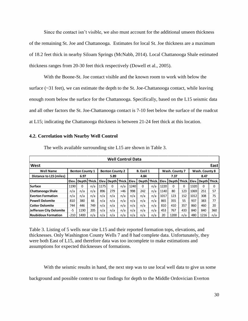
Since the contact isn’t visible, we also must account for the additional unseen thickness

of the remaining St. Joe and Chattanooga. Estimates for local St. Joe thickness are a maximum

of 18.2 feet thick in nearby Siloam Springs (McNabb, 2014). Local Chattanooga Shale estimated

thickness ranges from 20-30 feet thick respectively (Dowell et al., 2005).

With the Boone-St. Joe contact visible and the known room to work with below the

surface (~31 feet), we can estimate the depth to the St. Joe-Chattanooga contact, while leaving

enough room below the surface for the Chattanooga. Specifically, based on the L15 seismic data

and all other factors the St. Joe-Chattanooga contact is 7-10 feet below the surface of the roadcut

at L15; indicating the Chattanooga thickness is between 21-24 feet thick at this location.

4.2. Correlation with Nearby Well Control

The wells available surrounding site L15 are shown in Table 3.

Table 3. Listing of 5 wells near site L15 and their reported formation tops, elevations, and

thicknesses. Only Washington County Wells 7 and 8 had complete data. Unfortunately, they

were both East of L15, and therefore data was too incomplete to make estimations and

assumptions for expected thicknesses of formations.

With the seismic results in hand, the next step was to use local well data to give us some

background and possible context to our findings for depth to the Middle Ordovician Everton

Well Name

Distance to L15 (miles)

Elev. Depth Thick. Elev. Depth Thick. Elev. Depth Thick. Elev. Depth Thick. Elev. Depth Thick.

Surface 1190 0 n/a 1175 0 n/a 1240 0 n/a 1220 0 0 1320 0 0

Chattanooga Shale n/a n/a n/a 896 279 >46 998 242 n/a 1140 80 123 1069 251 57

Everton Formation n/a n/a n/a n/a n/a n/a n/a n/a n/a 1017 123 152 1012 308 75

Powell Dolomite 810 380 66 n/a n/a n/a n/a n/a n/a 865 355 55 937 383 77

Cotter Dolomite 744 446 749 n/a n/a n/a n/a n/a n/a 810 410 357 860 460 20

Jefferson City Dolomite -5 1190 205 n/a n/a n/a n/a n/a n/a 453 767 433 840 840 360

Roubidoux Formation -210 1400 n/a n/a n/a n/a n/a n/a n/a 20 1200 n/a 480 1216 n/a

6.97 5.89 4.84 7.37 8.47

Well Control Data

Benton County 1 Benton County 2 B. Ezeil 1 Wash. County 7 Wash. County 8

West East

31

Formation. The general idea was to use surrounding wells and their associated formation top data

to ascertain a general estimation of formation depth at site L15.

Unfortunately, only two wells (Washington County 7 &8) have information on Everton

Formation depth East of L15 (Table 3). These wells indicate the Everton Formation shallowing

westward, opposite of expectations. General structural trends would predict Everton deepening

to the west since this is the western flank of the Ozark Dome. Further, the Washington County

wells 7 & 8 Everton Formation top elevations were higher than the surface elevation of the

Boone Formation visible at L15. If the well data is accepted, it implies a significant down-to-the-

north fault in close proximity to the south of L15. According to the geologic map there is not a

fault recorded, but as we have noticed, it is in dense forest and may not have been extensively or

accurately mapped. This isn’t all that out of the ordinary though because according to Google

Earth pathway and elevation profiles the Boone Formation, visible at the L15, is roughly 200 feet

lower than what is seen at Washington County - 8 well in Tontitown, nearly 8 miles away. That

would mean over the east to west distance of roughly 8 miles away, there was only a depositional

dip of an estimated 0.47 degrees.

As mentioned previously, the L15 location sits in a graben to the east of a horst.

Elevations for formation tops as well as those exposed at the surface are different between this

horst and graben. To the east and west of the horst, formations such as the Chattanooga Shale are

not seen outcropping at the surface and are known mostly from well data.

The wells to the west of Pedro were not useful for our study. The other three wells

available to the west and south of the Pedro outcrop do not report formation top data to be used

for data correlation. Due to incomplete information, well control data were not sufficient to make

a prediction at the L15 site for thickness and depth values of the Everton.

32

4.3. Chattanooga Discussion

Depth estimation of the subsurface St. Joe-Chattanooga contact at L15 used seismic data,

local stratigraphy and deductive reasoning. The near surface seismic data indicate that the

Chattanooga-Everton contact is 69.5 feet below the surface at the survey location. The outcrop

face shows approximately 38 feet of visible outcrop based on a scaled photography (Figure 6).

The Everton top is about 31 feet below the surface at the base of the outcrop.

Chandler (2001) identified the Boone-St. Joe contact seen in the most eastern mound.

Chandler determined that the three olistolith or mound features used the Northview member as a

glide surface for transport to L15. This information indicates that below the visible surface, at

relatively shallow depth (inferred from the relative size of the blocks), shed by Bella Vista fault

the Northview member is present in the succession. Other research conducted in Benton County

by Manger (2012) and McNabb (2014) suggest that the St. Joe would have undergone condensed

sedimentation because of deposition in a deeper water setting. McNabb (2014) mentions that

observed beds thin in a southward direction from Jane, Missouri to Siloam Springs, Arkansas,

which further indicates evidence for condensed sedimentation.

The previous information leads me to believe that the St. Joe-Chattanooga contact is

within 7-10 feet of the ground surface at L15. This would leave 21-24 feet of Chattanooga before

the contact with the Everton. These estimates fit well with the seismic results at the site.

5. Conclusions

Near surface geophysical analysis was conducted to investigate subsurface formations at

the L15 roadcut near Pedro, Arkansas. Specifically, the targets of analysis were depth below

ground surface to the Ordovician Everton dolomite and indirect thickness estimation of

Devonian Chattanooga Shale. Well data in the vicinity of L15 was, unfortunately, not complete

33

enough to constrain the subsurface model. Thus, seismic analysis is the primary method that can

extend outcrop information at this location.

Manual seismic inversion resulted in a five-layer model as seen in Figure 6 and detailed

in Figure 10B. Primary results are (1) Everton Dolomite (18800 feet per second) occurs at

approximately 31 feet below surface at the foot of the L15 outcrop (at largest mound), and (2)

Chattanooga Shale thickness is 21-24 feet at this location. From the top of the outcrop, where the

survey was conducted, the Everton Formation is 69.5 feet below the surface.

The Chattanooga velocity is slower than in the confining formations, and therefore, the

top did not generate a refraction in our data. The Chattanooga Shale thickness was estimated to

be between 21-24 feet thick, based on nearby outcrops and constraints from the seismic model.

The determination of the Chattanooga-Everton formational contact is significant in that it

demonstrates that near surface seismic data can be used to reliably estimate the depth of buried

contacts and further extend the geological knowledge of Arkansas.

6. Future Research

Upon researching area geologic maps, it was determined from previous mapping that the

nearby area to L15’s west included two large faults running parallel in the northeast to southwest

direction straddling the town of Pedro, Arkansas. The main fault closest to L15 was the Bella

Vista fault and the second fault (further west) was a splay of the Bella Vista fault oriented almost

parallel to it. The Bella Vista fault and its splay created a horst that exposed the underlying

stratigraphic section that was not visible in outcrop at L15. It may benefit L15 to pursue further

research at this location and conduct near surface research in regard to the faulted area.

The process of conducting research for this experiment and manuscript has opened the

possibility for future research at L15 and the surrounding area. Some possible leads to follow

34

would be to conduct the survey again with a more powerful source or with a higher vertical stack

(more shots per shot location) to give a clearer picture of the data. This may lead to more

possible information about the mound features present in the outcrop as well as help to see

deeper into the near surface. Additional research that could be investigated would be to measure

section of nearby exposed Chattanooga as well as investigate other possible well data nearby to

help further confirm the survey results here at L15.

7. References

Bennison, A.P., 1986. Geological Highway Map of the Midcontinent Region Kansas, Missouri,

Oklahoma, Arkansas. American Association of Petroleum Geologists, Map 1, scale 1 inch

= approximately 32 miles.

Branner, J.C., 1891, Arkansas Geological Survey: http://www.geology.arkansas.gov/geology

/ozark_mississippian.htm (accessed March 2016)

Chandler, S.L., 2001, Carbonate Olistoliths, St. Joe and Boone Limestones (Lower

Mississippian) Northwest Arkansas: University of Arkansas, p.1-45

Cohen, J. K. and Stockwell, Jr. J. W., 2008, CWP/SU: Seismic Un*x, Release No. 44: an open

source software package for seismic research and processing, Center for Wave

Phenomena, Colorado School of Mines.

Docherty, P., 1991, Documentation for the 2.5D Common-Shot Modeling Program CSHOT,

Colorado School of Mines, Center for Wave Phenomena, CWT-U08R

Dowell, J.C., Hutchinson, C.M., Boss, S.K., 2005, Bedrock Geology of Rogers Quadrangle,

Benton County, Arkansas: Journal of Arkansas Academy of Science, v. 59, p. 56-64

Friesenhahn, T.C., 2010, Reservoir Characterization and Outcrop Analog the Osagean Reeds

Spring Formation (Lower Boone), Western Osage and Eastern Kay County, Oklahoma:

University of Arkansas, p. 29-44

Gasperikova, E., Morrison, F., “Seismic Velocity, Attenuation and Rock Properties” Berkley

Course in Applied Geophysics, University of California; Berkley, <http://appliedgeophys

ics.berkeley.edu/seismic/index.html> (accessed June 2017)

35

Haley, B.R. and the Arkansas Geological Commission Staff, Geologic Map of Arkansas, 1993.

“State Map Series, Arkansas Geological Survey.” Scale 1:500,000.

<http://www.geology.ar.gov/ark_state_maps/geologic.htm> (accessed 4/27/2017)

Haynes, C.W., 1891, Arkansas Geological Survey: <http://www.geology.arkansas.gov/geology

/ozark_devonian.htm> (Accessed March 2017)

Heiland, C.A., 1946, Geophysical Exploration, Prentice-Hall Inc., New York, New York, 1013p.

Liner, C.L., Liner, J. L., 1995, Ground-penetrating radar: A near-face experience from

Washington County, Arkansas: The Leading Edge, p. 17-21

Liner, C.L., Manger, W.L., Zachry, D., 2013, Mississippian Characterization Research in

Northwest Arkansas, AAPG Mid-Continent Meeting. Wichita, Kansas, PowerPoint. P.

18-21

Liner, C. L., 2016, Elements of 3D Seismology 3rd Edition, Society of Exploration

Geophysicists, 340p.

Liner, C.L., Personal Communication, 2017

Manger, W.L. 2012, An Introduction to the Lower Mississippian (Kinderhookian-Osagean)

Geology of the Tri-State Region, Southern Ozarks: Tulsa, Oklahoma, Halcon Resources

Corporation, p. 1-40

McCracken, M., 1971, Structural Features of Missouri, Missouri Geological Survey Report of

Investigations, number 49, 77p.

McGilvery, T., Manger, W.L., Zachry, D., 2016, The Carboniferous of Southwest Missouri and

Northwest Arkansas, Third Biennial Field Conference, AAPG Mid-Continent Section.

McNabb, A.L., 2014, High Resolution Stratigraphy of the St. Joe Group from Southwest

Missouri to Northeast Oklahoma: Oklahoma State University, p. 58, 105-107

Purdue, A.H., 1907, Arkansas Geological Survey: http://www.geology.arkansas.gov/geology/

ozark_ordovician.htm (Accessed March 2016)

Shelby, P.R., 1986, Depositional History of the St. Joe and Boone Formations in Northern

Arkansas, Proceedings, Arkansas Academy of Science: Fayetteville, AR, 1986, Vol 40, p.

67-71

Telford, W. M., Geldart, L. P., Sheriff, R. E. and Keys, D. A. 1976. Applied Geophysics.

Cambridge University Press. 860p.

36

Wolfram Research, Inc., 2016, Mathematica, Version 11.0, Champaign, IL

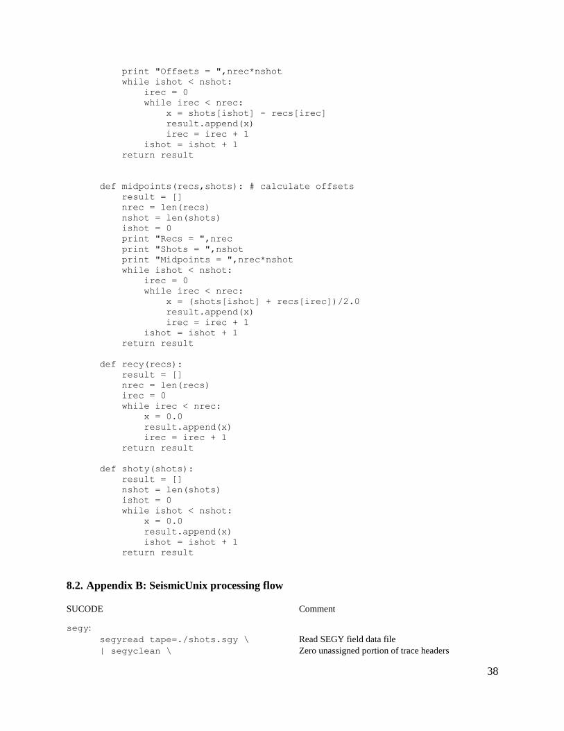
8. Appendices

8.1. Appendix A: Python code for 2D seismic survey design

Code 1: RunSeis.py

import matplotlib.pyplot as plt

import seis2d

# Credit: C. Liner April 2016

# seis2d.g(g0,dg,ng)

# g0 = first geophone x-coord

# dg = geophone spacing interval

# ng = number of geophones

# seis2d.s(s0,ds,ns)

# s0 = first shot x-coord

# ds = shot spacing interval

# ns = number of shots

# --- begin user input

# Pedro Ruggeri 3/21/2016

recs = seis2d.g(282.0,2.0,48)

shots = seis2d.s(0.0,8.0,85)

# --- end user input

# do not edit below this line

# print receiver and shot x-coordinates

print "receiver x-coordinates\n ",recs

print "shot x-coordinates\n ",shots

# calculate offsets

offsets = seis2d.offsets(recs,shots)

# calculate midpoints

midpoints = seis2d.midpoints(recs,shots)

# set receiver and shot y-coordinate to zero

gy = seis2d.recy(recs)

sy = seis2d.shoty(shots)

# plot shot/receiver layout

plt.figure(figsize=(28,6))

plt.scatter(recs,gy,marker='o',s=20, facecolors='none', edgecolors='b')

plt.scatter(shots,sy,marker='s',s=20, facecolors='none',edgecolors='r')

plt.xlabel('X-Distance (ft)')

plt.ylabel('Y-Distance (ft)')

plt.title('Shots and Receivers')

plt.grid(True)

# plot offsets

plt.figure(figsize=(9,6))

plt.plot(sorted(offsets),'ro',markersize=3,markeredgecolor='r')

plt.ylabel('Offset (ft)')

37

plt.xlabel('Trace')

plt.title('Trace offsets')

plt.grid(True)

# plot midpoints

plt.figure(figsize=(9,6))

plt.plot(sorted(midpoints),'ro',markersize=3,markeredgecolor='r')

plt.ylabel('Midpoint X-Coord (ft)')

plt.xlabel('Trace')

plt.title('Trace midpoint')

plt.grid(True)

plt.show()

Code 2: seis2d.py

# 2D seismic design module

# x-coordinate origin at left-most shot or rec and increasing right

# Credit: C. Liner April 2016

def g(g0,dg,ng): # receiver x-coordinates

# g0 = first receiver x location

# dg = receiver interval

# ng = number of receivers

result = []

x = g0

ix = 0

while ix < ng:

result.append(x)

x = x + dg

ix = ix + 1

print "Receiver x-coordinates"

return result

def s(s0,ds,ns): # shot x-coordinates

# s0 = first shot x location

# ds = shot interval

# ns = number of shots

result = []

x = s0

ix = 0

while ix < ns:

result.append(x)

x = x + ds

ix = ix + 1

print "Shot x-coordinates"

return result

def offsets(recs,shots): # calculate offsets

result = []

nrec = len(recs)

nshot = len(shots)

ishot = 0

print "Recs = ",nrec

print "Shots = ",nshot

38

print "Offsets = ",nrec*nshot

while ishot < nshot:

irec = 0

while irec < nrec:

x = shots[ishot] - recs[irec]

result.append(x)

irec = irec + 1

ishot = ishot + 1

return result

def midpoints(recs,shots): # calculate offsets

result = []

nrec = len(recs)

nshot = len(shots)

ishot = 0

print "Recs = ",nrec

print "Shots = ",nshot

print "Midpoints = ",nrec*nshot

while ishot < nshot:

irec = 0

while irec < nrec:

x = (shots[ishot] + recs[irec])/2.0

result.append(x)

irec = irec + 1

ishot = ishot + 1

return result

def recy(recs):

result = []

nrec = len(recs)

irec = 0

while irec < nrec:

x = 0.0

result.append(x)

irec = irec + 1

return result

def shoty(shots):

result = []

nshot = len(shots)

ishot = 0

while ishot < nshot:

x = 0.0

result.append(x)

ishot = ishot + 1

return result

8.2. Appendix B: SeismicUnix processing flow SUCODE Comment

segy: segyread tape=./shots.sgy \ Read SEGY field data file | segyclean \ Zero unassigned portion of trace headers

39

> shots.su Create output file surange < shots.su > range.txt Scan trace headers and save as text file

sugain < shots.su agc=1 wagc=0.1 \ Apply 0.1 sec automatic gain control (AGC)

| suximage perc=99 & Display the data

hdr:

# 85 shots into 48 receivers Comment # shot interval 8 ft, receiver

interval 2 ft

# First shot defines x=0

sushw < shots.su key=tracl a=1 Set trace header word, 1,2,3,… c=1 j=1 \

| sushw key=sx a=0 c=8 j=48 \ Set shot coord. 1st 48=0, 2nd 48=8… | sushw key=gx a=282 b=2 j=48 \ Rec. coord. 282 + 2ft step | suazimuth \ Set offset and midpoint header words

offset=1 signedflag=1 \ Offsets are positive and negative cmp=1 mxkey=cdp mykey=ep \ Set cmp header word

> shots1.su Output data file surange < shots1.su Scan trace headers to terminal

ostk:

susort < shots1.su offset \ Sort data by offset

| sustack key=offset \ Stack data across equal offsets

> ostk.su Output offset stack data

sugain < ostk.su \ Gain the offset stack data

agc=1 wagc=0.1 \ AGC with 0.1 sec window

| suxwigb key=offset \ Display data as interactive wiggle plot f1=-0.005 \ First time is -0.005 sec, manual shift data grid1=dot grid2=dot \ Make gridlines on both axes dotted

windowtitle="Shot offset stack" \ Window label perc=98 & Display gain, 2% clip sugain < ostk.su \ Gain the offset stack data agc=1 wagc=0.1 \ AGC with 0.1 sec window

| suximage perc=98 \ Display data as interactive image f2=0 d2=2 label2="Offset (ft)" \ x-axis:start 0, step 2, label offset in feet f1=-5 d1=0.25 \ t-axis:start -5 ms, step 0.25 ms

x1beg=0 f1num=0 d1num=10 \ t-axis:begin 0, 1st label 0, label step 10ms

label1="Time (msec)" \ t-axis label

grid1=dot grid2=dot \ Make gridlines on both axes dotted

windowtitle="Shot offset stack" & Window title run in background

sugain < ostk.su \ Gain the offset stack data

agc=1 wagc=0.1 \ AGC with 0.1 sec window | supsimage perc=98 \ Display as postscript image

f1=-5 d1=0.25 \ t-axis:start -5 ms, step 0.25 ms

x1beg=0 f1num=0 d1num=10 \ t-axis:begin 0, 1st label 0, label step 10ms

label1="Time (msec)" \ t-axis label f2=-390 d2=2 \

f2num=-350 d2num=50 \

label2="Offset (ft)" \

d2s=0.1 \

grid1=dot grid2=dot \ Both axes gridlines dotted

40

labelsize=14 \

title="Pedro 3-21-16" \

> fig1.eps Write postscript file

ps2pdf fig1.eps Convert postscript to pdf

sugain < ostk.su \ Gain the offset stack data agc=1 wagc=0.1 \ AGC with 0.1 sec window

| suwind key=offset max=0 \ Keep only negative offsets | supsimage perc=98 \ Display as postscript image f2=-390 d2=2 \ Plotting parameters (and below) f2num=-240 d2num=20 \

x2beg=-250 \

label2="Offset (ft)" \

d2s=0.1 \

f1=-5 d1=0.25 \

x1beg=0 x1end=100 \ d1num=5 \

label1="Time (msec)" \

grid1=dot grid2=dot \

labelsize=14 \

title="Pedro 3-21-16" \

> fig2.eps Write postscript file ps2pdf fig2.eps Convert postscript to pdf

rm *.eps Remove all postscript files

8.3. Appendix C: MathematicaTM code for interactive seismic refraction fitting

WORKFLOW

1. Pick linear first breaks from shot record and put results in file named firstbreak.csv (CSV

format) as (offset, time) pairs. Units of offset determine units of velocity.

2. Run GET DATA cell to load (offset, time) pairs into data list. Rename plot by changing name

string.

3. Run FIT DATA cell

4. Adjust Max Offset and Max Time till all data points are visible

5. Adjust layer 1 velocity to fit direct arrival points (should pass through origin)

6. Adjust layer 2 velocity until parallel to 2nd linear trend, then adjust layer 1 thickness to pass

through center of data points

7. If 3rd trend is present: Adjust layer 3 velocity until parallel to 3rd linear trend, then adjust

layer 2 thickness to pass through center of data points

8. If 4th trend is present: Adjust layer 4 velocity until parallel to 4th linear trend, then adjust

layer 3 thickness to pass through center of data points

REFERENCES

W. M. Telford, L. P. Geldart, R. E. Sheriff, & D. A. Keys 1976. Applied Geophysics, xvii + 860

pp., numerous figs. Cambridge University Press, pages 278-281 ClearAll["Global`*"]

41

(* get data *)

mdata = Import[NotebookDirectory[], "firstbrk.csv"];

tshift = 0.007;

data =

Table[{mdata[[i]][[2]], mdata[[i]][[1]] - tshift}, {i, 1, Length[mdata]}]

dname = "Pedro Ruggeri 3/21/2016";

(* fit data *)

Manipulate[

(* direct wave arrival *)

t0 := x/v1;

(* refr arrival from interface 1 *)

t1 := x/v2 + (2 z1 Cos[a1c])/ v1;

(* refr arrival from interface 2 *)

t2 := x/v3 + (2 z2 Cos[a2c])/v2 + (2 z1 Cos[a1])/ v1;

(* refraction arrival from interface 3 *)

t3 := x/v4 + (2 z3 Cos[a3c])/v3 + (2 z2 Cos[a2])/v2 + (2 z1 Cos[a1])/v1;

(* critical incidence angle for interface 1 *)

a1c := ArcSin[v1/v2];

(* incidence angle on interface 1 *)

a1 := ArcSin[v1/v3];

(* critical incidence angle for interface 2 *)

a2c := ArcSin[v2/v3];

(* incidence angle on interface 2 *)

a2 := ArcSin[v2/v4];

(* critical incidence angle for interface 3 *)

a3c := ArcSin[v3/v4];

Show[{ListPlot[data,

PlotStyle -> {PointSize[0.025], Red},

PlotRange -> {{0, xmax}, {0, tmax}}],

Plot[{t0, t1, t2, t3}, {x, 0, xmax},

PlotStyle -> Thick,

PlotRange -> {{0, xmax}, {0, tmax}}]},

FrameStyle -> (FontFamily -> "Helvetica"),

LabelStyle -> (FontFamily -> "Helvetica"),

BaseStyle -> {FontSize -> 12},

FrameLabel -> {"Offset (ft)", "Time (sec)"},

GridLines -> Automatic,

GridLinesStyle -> Directive[Dashed],

PlotLabel -> dname <> "\nFirst Break Interpretation",

ImageSize -> 400,

Axes -> False,

Frame -> True],

"Layer 1",

{{v1, 1640, " Velocity (ft/s)"}, 200, 6000, 5, Appearance -> "Labeled"},

{{z1, 5, " Thickness (ft)"}, .1, 100, Appearance -> "Labeled"},

Delimiter, "Layer 2",

{{v2, 6840, " Velocity (ft/s)"}, 200, 15000, Appearance -> "Labeled"},

{{z2, 9.9, " Thickness (ft)"}, 2, 100, Appearance -> "Labeled"},

Delimiter, "Layer 3",

{{v3, 12880, " Velocity (ft/s)"}, 200, 20000, Appearance -> "Labeled"},

{{z3, 15.5, " Thickness (ft)"}, 2, 100, Appearance -> "Labeled"},

Delimiter, "Layer 4 (set v=200 for 3-layer fit)",

{{v4, 16360, " Velocity (ft/s)"}, 200, 20000, Appearance -> "Labeled"},

Delimiter, "Plotting Parameters",

{{xmax, 240, " Max Offset (ft)"}, 5, 1000, Appearance -> "Labeled"},

42

{{tmax, .06, " Max Time (s)"}, .001, 0.5, Appearance -> "Labeled"},

Delimiter,

Style["Credit: Prof. C. Liner, U Arkansas (15 Sept 2014)", Italic],

ControlPlacement -> Left

]