the physical properties of fermi tev bl lac objects jets · we investigate the physical properties...

arX

iv:1

609.

0570

4v1

[ast

ro-p

h.H

E]

19 S

ep 2

016

Mon. Not. R. Astron. Soc.000, 000–000 (0000) Printed 29 September 2018 (MN LATEX style file v2.2)

The physical properties ofFermi TeV BL Lac objects jets

N. Ding1, X. Zhang1⋆, D. R. Xiong2, H. J. Zhang11Department of physics, Yunnan Normal University, Kunming 650500, China2Yunnan observatories, Chinese Academy of Sciences, Kunming 650011, China

29 September 2018

ABSTRACTWe investigate the physical properties ofFermi TeV BL Lac objects jets by modeling thequasi-simultaneous spectral energy distribution of 29Fermi TeV BL Lacs in the frame of aone-zone leptonic synchrotron self-Compton model. Our main results are the following: (i)There is a negative correlation betweenB andδ in our sample, which suggests thatB andδare dependent on each other mainly in Thomson regime. (ii) There are negative correlationsbetweenνsy andr, theνIC andr, which is a signature of the energy-dependence statisticalacceleration or the stochastic acceleration. There is a significant correlation betweenr ands,which suggests that the curvature of the electron energy distribution is attributed to the energy-dependence statistical acceleration mechanism. (iii) By assuming one proton per relativisticelectron, we estimate the jet power and radiative power. A size relationPe ∼ Pp > Pr & PBis found in our sample. ThePe > PB suggests that the jets are particle dominated, and thePe ∼ Pp means that the mean energy of relativistic electrons approachesmp/me. There arenot significant correlations betweenPjet and black hole mass in high or low state with a sub-sample of 18 sources, which suggests that the jet power weakly depends on the black holemass. (iv) There is a correlation between the changes in the flux density at 1 TeV and thechanges in theγpeak, which suggests the change/evolution of electron energy distribution maybe mainly responsible for the flux variation.

Key words: galaxies: BL Lacertae objects - galaxies: active - galaxies: jets - radiation mech-anisms: non-thermal

1 INTRODUCTION

Blazars are the most extreme active galactic nuclei (AGNs) point-ing their jets in the direction of the observer (Urry & Padovani1995). They have high luminosity, large amplitude and rapidvari-ability, high and variable polarization, radio core dominance, andapparent super-luminal speeds (Urry & Padovani 1995; Massaro etal. 2016). Generally, Blazars are divided into subcategories of BLLacs objects (BL Lacs), characterized by almost completelylack-ing of emission lines or only showing weak emission lines (EW6 5 A), and highly polarized quasars or flat spectral radio quasars(FSRQs), showing broad strong emission lines (Falomo et al.2014;Massaro et al. 2014). The broadband spectral energy distributions(SEDs) of blazars are double peaked. The bump at the IR-optical-UV band is explained with the synchrotron emission of relativisticelectrons, and the bump at the GeV-TeV gamma-ray band is due tothe inverse Compton (IC) scattering (e.g., Dermer et al. 1995; Der-mer et al. 2002; Böttcher 2007). The seed photons for IC processcould be from the local synchrotron radiation on the same relativis-tic electrons (i.e. synchrotron self-Compton (SSC); e.g.,Tavecchioet al. 1998), or from the external photon fields (EC; e.g., Dermer

⋆ E-mail:[email protected]

et al. 2009), such as those from accretion disk (e.g., Dermer&Schlickeiser 1993) and broad-line region (e.g., Sikora et al. 1994).The hadronic model is an alternative explanation for the high en-ergy emissions from blazars (e.g., Dermer et al. 2012).

The modeling of SED with a given radiation mechanism al-low us to investigate the intrinsic physical properties of emittingregion and the physical conditions of jet (e.g., Ghisellini& Tavec-chio 2008; Celotti & Ghisellini 2008; Ghisellini et al. 2009; Ghis-ellini et al. 2010; Ghisellini et al. 2011; Zhang et al. 2012;Yan et al.2014). Celotti & Ghisellini (2008) estimated the powers of blazarsjets based on EGRET observations and they found that the typicaljet should comprise an energetically dominant proton componentand only a small fraction of the jet power is radiated if thereis oneproton per relativistic electron. In addition, in their work, the TeVBL Lacs shows some special jet properties, such asPe ∼ Pp andrelatively high radiation efficiency. Ghisellini et al. (2009, 2010,2011) mainly concerned the relation between the jet power and theaccretion disk luminosity inFermi blazars and they found that thereis a positive correlation between the jet power and the accretiondisk luminosity forFermi broad-line blazars.

Theγ-ray extragalactic sky at high (> 100 MeV) and very high(> 100 GeV) energies is dominated by blazars. About 50 blazars

c© 0000 RAS

http://arxiv.org/abs/1609.05704v1

2 N. Ding, X. Zhang, D. R. Xiong, H. J. Zhang

have been detected in the TeV gamma-ray band1, and most of themare the BL Lacs. The SEDs of TeV BL Lacs suffer less contami-nation of the emission from the accretion disk and EC process, soit can be explained well by the one-zone SSC model (Paggi et al.2009a; Dermer et al. 2015). Since the launch of theFermi satellite,we have entered in a new era of blazar research (Abdo et al. 2009;Abdo et al. 2010a). The abundant data observed byFermi/LAT inthe MeV-GeV band, together with the multi-wavelength campaignsat the radio, optical, X-ray bands and the ground-based observa-tions at the TeV gamma-ray band, now provide an excellent oppor-tunity to study the TeV blazars (e.g., Massaro et al. 2011a, Giommiet al. 2012; Massaro et al. 2013).

In this paper, we have collected the quasi-simultaneous broad-band SEDs of 29Fermi TeV BL Lacs from the literatures. Weused the one-zone leptonic synchrotron self-Compton modelwiththe log-parabolic electron energy distribution to fit SEDs.And weused the Markov Chain Monte Carlo sampling method instead ofthe "eyeball" fitting to obtain the best-fit model parameters. Then,based on the model parameters, we systematically investigated thephysical properties ofFermi TeV BL Lacs jets through statisticalanalysis. This paper is organized as follows: In Sect.2, we presentthe sample, the model and the fitting strategy are presented inSect.3. Then, results and discussions are showed in Sect.4.Finally,we end with a conclusion of the findings in Sect.5. The cosmo-logical parametersH0 = 70 Km s−1Mpc−1, Ωm = 0.3, andΩΛ = 0.7 are adopted in this work.

2 THE SAMPLE

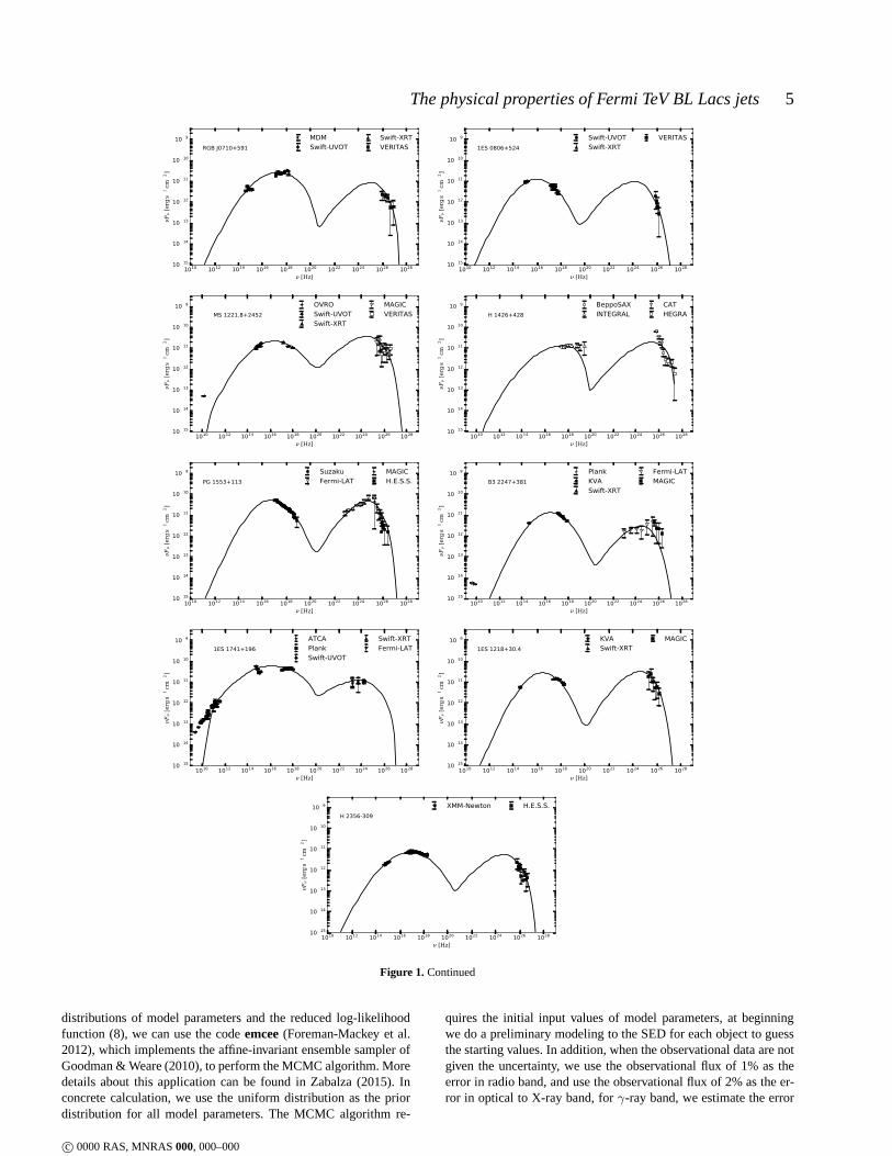
Up to now, 55 BL Lacs have been detected in the TeV or very highenergy regime1. 46 of them have been detected at MeV-GeV en-ergies byFermi/LAT. In order to study the physical properties ofFermi TeV BL Lacs jets, we have collected the quasi-simultaneousbroadband SEDs of 29Fermi TeV BL Lacs from the literatures.For each source, the time of quasi-simultaneous observation, theobservation telescopes, and the references are listed in Table 1. Oursample accounts for about 65% of the total number ofFermi TeVBL Lacs. There are 12 sources which have two broadband SEDs.The two SEDs for 12 sources are defined as a high or low state withthe observed or extrapolated flux density at 1 TeV. The observedbroadband SEDs are shown in Figure 1.

3 MODELING FITTING PROCEDURE

3.1 Model

We adopt a one-zone leptonic SSC model. And we assume the elec-tron energy distribution is a log-parabolic spectra (Massaro et al.2004a; Tramacere et al. 2011),

N(γ) = N0(γ

γ0)−s−rlog(

γγ0

)= NK(

γ

γ0)−s−rlog(

γγ0

). (1)

K is the normalization coefficient,∫ γmax

γmin

K(γ

γ0)−s−rlog(

γγ0

) = 1. (2)

N is the number of emitting particles per unit volume expressed in1/cm3. γ0 is the reference energy.r is the spectral curvature.s isthe spectral index at the reference energyγ0. γmin andγmax are the

1 http://tevcat.uchicago.edu/.

minimum and maximum energies of electrons. The log-parabolicelectron energy distribution can be obtained from a Fokker-Planckequation as first shown by Kardashev(1962). The log-parabolicelectron energy distribution provides more accurate fits than brokenpower-laws in the optical X-ray bands, with residuals uniformlylow throughout a wide energy range (Paggi et al. 2009a). Recently,the log-parabolic electron energy distribution has also been appliedto describe the spectral distribution and evolution of somegamma-ray bursts (Massaro & Grindlay 2011).

The radiation region is taken as a homogeneous sphere withradiusR and filled with the uniform magnetic fieldB. Due to thebeaming effect, the observed radiation is strongly boostedby rel-ativistic Doppler factorδ. The synchrotron emission coefficient iscalculated with

jsyn(ν) =1

4π

∫ γmin

γmin

N(γ)P (ν, γ)dγ, (3)

and the synchrotron absorption coefficient is calculated with

αsyn(ν) = −1

8πν2me

∫ γmax

γmin

dγP (ν, γ)γ2 ∂

∂γ[N(γ)

γ2]. (4)

WhereP (ν, γ) is the single electron synchrotron emission aver-aged over an isotropic distribution of pitch angles (see, e.g., Ghis-ellini et al. 1988),me is electron mass. According to the radiativetransfer equation of spherical geometry, we can calculate the syn-chrotron radiation intensity,

Isyn(ν) =jsyn(ν)

αsyn(ν)[1−

2

τ (ν)2(1− τe−τ(ν)

− e−τ(ν))], (5)

whereτ (ν) = 2Rαsyn(ν). The IC emission coefficient is calcu-lated with

jIC(ǫ) =hǫ

4π

∫dǫ0n(ǫ0)

∫γN(γ)C(ǫ, γ, ǫ0), (6)

whereǫ is scattered photon energy andǫ0 is soft photon energy (inunit of mec

2). C(ε, γ, ǫ0) is the Compton kernel of Jones (1968),n(ǫ0) is the number density of synchrotron soft photons per en-ergy interval. More detailed calculation process see Kataoka et al.(1999). Due to the medium is transparent for IC radiation, henceIIC(ν) = jIC(ν)R.

Assuming thatIsyn, IC is an isotropic radiation field, the totalobserved flow density is given by

Fobs(νobs) =πR2δ3(1 + z)

d2L(Isyn(ν) + IIC(ν)), (7)

wheredL is the luminosity distance,z is the redshift, andνobs =νδ/(1 + z). In addition, the high-energy gamma-ray photons canbe absorbed by extragalactic background light (EBL), yieldingelectron-positron pairs. It makes the observed spectrum inthe veryhigh energy (VHE) band must be steeper than the intrinsic one.Therefore, according to the average EBL model in Dwek & Kren-nrich (2005), we calculate the absorption in the GeV-TeV band.

3.2 Fitting strategy

In this model, there are nine free parameters. Six of them spec-ify the electron energy distribution (N, γmin, γmax, γ0, r, s), andother three ones describe the properties of the radiation region(R,B, δ). For a given source, we calculate its non-thermal fluxto fit the observed multi-wavelength data. We derive the best-fitand uncertainty distributions of model parameters throughMarkov

c© 0000 RAS, MNRAS000, 000–000

The physical properties of Fermi TeV BL Lacs jets 3

1010 1012 1014 1016 1018 1020 1022 1024 1026 1028

ν [Hz]

10−15

10−14

10−13

10−12

10−11

10−10

10−9

10−8

νFν [erg s−1 cm

−2]

1ES 1101-232SuzakuH.E.S.S.XMM-Newton

RXTEH.E.S.S.

1010 1012 1014 1016 1018 1020 1022 1024 1026 1028

ν [Hz]

10015

10014

10013

10012

10011

10010

1009

1008

1007

νFν [erg s−1 m

−2]

Mkn421

FLWORXTEWhipple

Swif−-UVOTSwift-XRTSwift-BAT

Fermi-LATMAGIC

1010 1012 1014 1016 1018 1020 1022 1024 1026 1028

ν [Hz]

10−15

10−14

10−13

10−12

10−11

10−10

10−9

10−8

10−7

νFν [erg s−1 cm

−2]

Mkn501

Bepp SAXCATKVA

SuzakuMAGIC

1010 1012 1014 1016 1018 1020 1022 1024 1026 1028

ν [H2]

10−15

10−14

10−13

10312

10311

10310

1039

1038

1037

1036

νFν [erg s−1 m

−2]

1ES 1959+650

Boltwood Observatory and Abastumani ObservatoryRXTEHEGRA

Swift-UVOTSuzakuMAGIC

1010 1012 1014 1016 1018 1020 1022 1024 1026 1028

ν [Hz]

10−15

10−14

10−13

10−12

10−11

10−10

10−9

10−8

10−7

10−6

νFν [erg s−1 cm

−2]

PKS 2005-489

Swift-UVOTRXTE and Swift-XRT

H.E.S.S.XMM-Newton

1011 1013 1015 1017 1019 1021 1023 1025 1027

ν [Hz]

10−15

10−14

10−13

10−12

10−11

10−10

10−9

10−8

10−7

10−6

νFν [erg s−1 m

−2]

PKS 2155-304

Bronberg ObservatoryRXTEChandra and H.E.S.S.ATOM

RXTEFermi-LATH.E.S.S.

1010 1012 1014 1016 1018 1020 1022 1024 1026 1028

ν [Hz]

10−14

10−13

10−12

10−11

10−10

10−9

10−8

νFν [er s−1 cm

−2]

1ES 2344+514

Swift-UVOTSwift-XRTVERITAS

KVASwift-XRTMAGIC

1010 1012 1014 1016 1018 1020 1022 1024 1026 1028

ν [Hz]

10−14

10−13

10−12

10−11

10−10

10−9

10−8

10−7

νFν

[erg

s−1 c

m−2]

W ComSw ft-UVOTSwift-XRTVERITASAAVSO

Swift-UVOTSwift-XRTFermi-LATVERITAS

1010 1012 1014 1016 1018 1020 1022 1024 1026 1028

ν [Hz]

10−14

10−13

10−12

10−11

10−10

10−9

10−8

νFν [er s−1 cm

−2]

S5 0716+714

KVASwift-XRTMAGIC

Swift-UVOTSwift-XRT

1010 1012 1014 1016 1018 1020 1022 1024 1026 1028

ν [Hz]

10214

10213

10212

10211

10210

1029

1028

νFν [erg s−1 cm

−2]

BL L c

KVA

EGRET

MAGIC

Effelsberg Observ −or0

Swif−-UVOT GASP-WEBT Collaboration

Swift-XRT

Fermi-LAT

Figure 1. The observed SEDs (scattered data points) with our best model fittings (lines) of 29Fermi TeV BL Lacs. The data of high and low states are markedwith blue and red symbols, respectively. If only one SED is obtained, the data are shown with black symbols. The open symbols are for the data obtained notin the time of quasi-simultaneous observation, the detailed information about the data sets are listed in Table 1. For Mkn180, 3C 66A, PKS 1424+240 and 1ES1215+303, the red dashed lines are calculated by the on-lineSSC calculator (see text in detail).

c© 0000 RAS, MNRAS000, 000–000


1010 1012 1014 1016 1018 1020 1022 1024 1026 1028

ν [Hz]

10−14

10−13

10−12

10−11

10−10

10−9

10−8

νFν [er s−1 cm

−2]

1ES 1011+496

Swift-UVOTSwift-XRTMAGICOVRO

Swift-UVOTSwift-XRTFermi-LAT

1010 1012 1014 1016 1018 1020 1022 1024 1026 1028

ν [Hz]

10−14

10−13

10−12

10−11

10−10

10−9

10−8

νFν

[erg

s−1 c

m−2]

MAGIC J2001+435

Swi t-UVOTSwift-XRTMAGICOVRO


1010 1012 1014 1016 1018 1020 1022 1024 1026 1028

ν [Hz]

10−13

10−12

10−11

10−10

νFν [ergs−

1cm

−2]

Mkn180

Swift-UVOTSwift-XRTMAGIC

1010 1012 1014 1016 1018 1020 1022 1024 1026 1028

ν [Hz]

10−13

10−12

10−11

10−10

10−9

10−8

νFν [ergs−

1cm

−2]

3C 66A

MDMSwif -UVOTSwift-XRT

Fermi-LATVERITAS

1010 1012 1014 1016 1018 1020 1022 1024 1026 1028

ν [Hz]

10−13

10−12

10−11

10−10

10−9

νFν [ergs−

1cm

−2]

PKS 1424+240MDMSwift-UVOTSwift-XRT

Fermi-LATVERITAS

1010 1012 1014 1016 1018 1020 1022 1024 1026 1028

ν [Hz]

10−13

10−12

10−11

10−10

10−9

νFν

[ergs−

1cm

−2]

1ES 1215+303Metsahov KVASw ft-UVOT

Swift-XRTFermi-LATVERITAS

1011 1013 1015 1017 1019 1021 1023 1025 1027 1029

ν [Hz]

10 13

10 12

10 11

10 10

νFν [ergs−

1cm

−2]

1RXS J003334.6-192130


1010 1012 1014 1016 1018 1020 1022 1024 1026 1028

ν [Hz]

10−13

10−12

10−11

10−10

νFν [ergs−

1cm

−2]

RGB J0152+017

RXTESwift-XRTH.E.S.S.

1010 1012 1014 1016 1018 1020 1022 1024 1026 1028

ν [Hz]

10−15

10−14

10−13

10−12

10−11

10−10

νFν [ergs−

1cm

−2]

1ES 0414+009 MDMS ift-XRT

Fermi-LATVERITAS

1010 1012 1014 1016 1018 1020 1022 1024 1026 1028

ν [Hz]

10−15

10−14

10−13

10−12

10−11

10−10

10−9

νFν [ergs−

1cm

−2]

PKS 0447-439

Swift-UVOTSwift-XRT

Fermi-LATVERITAS

Figure 1. Continued

Chain Monte Carlo (MCMC) sampling of their likelihood distribu-tions. When measurements and uncertainties in the observedmulti-wavelength data are assumed to be correct, Gaussian, and indepen-dent. The reduced log-likelihood of observed data given themodel

flux S(~p, ν), for a parameter vector~p, is

lnL ∝

N∑i=1

(S(~p, νi)− Fi)2

σ2i

, (8)

whereFi, σi are the flux measurement and uncertainty at a fre-quencyνi over N spectral measurements. Combining the prior

c© 0000 RAS, MNRAS000, 000–000


1010 1012 1014 1016 1018 1020 1022 1024 1026 1028

ν [Hz]

10−15

10−14

10−13

10−12

10−11

10−10

10−9

νFν [ergs−

1cm

−2]

RGB J0710+591

MDMSwif -UVOT

Swift-XRTVERITAS

1010 1012 1014 1016 1018 1020 1022 1024 1026 1028

ν [Hz]

10−15

10−14

10−13

10−12

10−11

10−10

10−9

νFν [ergs−

1cm

−2]

1ES 0806+524

Swift-UVOTSwift-XRT

VERITAS

1010 1012 1014 1016 1018 1020 1022 1024 1026 1028

ν [Hz]

10 15

10 14

10 13

10 12

10 11

10 10

10 9

νFν [ergs−

1cm

−2]

MS 1221.8+2452

OVROSwift-UVOTSwift-XRT

MAGICVERITAS

1010 1012 1014 1016 1018 1020 1022 1024 1026 1028

ν [Hz]

10−15

10−14

10−13

10−12

10−11

10−10

10−9

νFν [ergs−

1cm

−2]

H 1426+428

BeppoSAXINTEGRAL

CATHEGRA

1010 1012 1014 1016 1018 1020 1022 1024 1026 1028

ν [Hz]

10−15

10−14

10−13

10−12

10−11

10−10

10−9

νFν [ergs−

1cm

−2]

PG 1553+113

SuzakuFe mi-LAT

MAGICH.E.S.S.

1010 1012 1014 1016 1018 1020 1022 1024 1026 1028

ν [Hz]

10−15

10−14

10−13

10−12

10−11

10−10

10−9

νFν

[ergs−

1cm

−2]

B3 2247+381

PlankKVASwi t-XRT

Fermi-LATMAGIC

1010 1012 1014 1016 1018 1020 1022 1024 1026 1028

ν [Hz]

10−15

10−14

10−13

10−12

10−11

10−10

10−9

νFν [ergs−

1cm

−2]

1ES 1741+196

ATCAPlan Swift-UVOT

Swift-XRTFermi-LAT

1010 1012 1014 1016 1018 1020 1022 1024 1026 1028

ν [Hz]

10−15

10−14

10−13

10−12

10−11

10−10

10−9

νFν [ergs−

1cm

−2]

1ES 1218+30.4

KVASwift-XRT

MAGIC

1010 1012 1014 1016 1018 1020 1022 1024 1026 1028

ν [Hz]

10−15

10−14

10−13

10−12

10−11

10−10

10−9

νFν [ergs−

1cm

−2]

H 2356-309

XMM-Newton H.E.S.S.

Figure 1. Continued

distributions of model parameters and the reduced log-likelihoodfunction (8), we can use the codeemcee(Foreman-Mackey et al.2012), which implements the affine-invariant ensemble sampler ofGoodman & Weare (2010), to perform the MCMC algorithm. Moredetails about this application can be found in Zabalza (2015). Inconcrete calculation, we use the uniform distribution as the priordistribution for all model parameters. The MCMC algorithm re-

quires the initial input values of model parameters, at beginningwe do a preliminary modeling to the SED for each object to guessthe starting values. In addition, when the observational data are notgiven the uncertainty, we use the observational flux of 1% as theerror in radio band, and use the observational flux of 2% as theer-ror in optical to X-ray band, forγ-ray band, we estimate the error

c© 0000 RAS, MNRAS000, 000–000


Figure 2. The posterior distributions of model parameters for Mrk180obtained through the MCMC sampling. The dotted lines are themedian lines. we usethe posterior medians as the best-fit values and estimate uncertainties based on the 16th and 84th percentiles.

with the average relative error of the data points whose errors areavailable (Zhang et al. 2012; Aleksic et al. 2014a).

The minimum energy of electronsγmin is historically poorlyconstrained by SED modeling, especially for low-power BL Lacs(Celotti & Ghisellini 2008). The same as the previous studies (Raniet al. 2011; Yan et al. 2014; Kang et al. 2016), we use a fixedγmin inour fitting. Due to the synchrotron self-absorption, the radio emis-sion cannot be used to constrain the value ofγmin. However, theobserved spectral index between the X-ray and theγ-ray and theGeV data at low energies could place constraints onγmin in somedegree (Tavecchio et al. 2000; Yan et al. 2014). According totheaverage observed spectral index between the X-ray and theγ-rayof the high peaked frequency BL LacsαXγ=1.02 (Fan et al. 2012)and the GeV data at low energies, we do a preliminary modelingto the SED for each object. Based on the preliminary modelingre-sult, theγmin = 10 are adopted in our fitting. Figure 2 shows theposterior distributions of model parameters for Mrk180 obtainedthrough the MCMC sampling. We use the posterior medians as thebest-fit values and estimate uncertainties based on the 16thand 84thpercentiles.

4 RESULTS AND DISCUSSION

Using above mentioned model and fitting strategy, we fit the 29Fermi TeV BL Lacs and obtain their best-fit model parameters (seeFigure 1 and Table 2). Due to the synchrotron self-absorption, theone-zone SSC emission will fall in the radio band. It leads totheobserved data in the radio band can not be well fitted. The one-zoneSSC model here adopted is aimed to explain the bulk of the emis-sion in compact radiation regions, but the radio flux mainly comesfrom a large-scale radiation regions outside the jet, so theradio dataare not restricted by the one-zone SSC model, meanwhile, thebadfitting in the radio band does not affect the determination ofmodelparameters (Ghisellini et al. 2009; Ghisellini et al. 2010).

Tramacere et al. provided an on-line SSC calculator2 (Tra-macere et al. 2007a, 2009). We use the same model parameters tocalculate SSC emission by using this on-line SSC calculatorforMkn180, 3C 66A, PKS 1424+240 and 1ES 1215+303. The results

2 http://www.isdc.unige.ch/sedtool/.

are plotted as the red dashed lines in Figure 1. It can be foundthatthe results are similar to ours, which proves that our SSC codeis reliable. The minor differences in results are mainly caused bythe different approximation methods for Bessel function. In ourwork, we use the approximate method proposed by Aharonian etal. (2010), the approximation error is less than 0.2%.

4.1 The distributions

In Figure 3, we give the distributions of the spectral curvaturer andthe spectral indexs. It is found that the range ofr are from 0.30 to1.21, the values ofs are clustered at 1.10∼ 2.30. The mean valuesof r ands are 0.79 and 1.85, respectively.

We show the distributions ofR, B, andδ in Figure 4. Thevalues ofR are in the range of (0.7∼ 40) × 1015 cm, which isconsistent with Zhang et al (2012). The values of magnetic field inthe emitting regionB are in the range of 0.1∼ 1 G, which is consis-tent with Ghisellini et al. (2011) and Zhang et al.(2012). The valuesof δ are in the range of 8∼ 38, which is similar to the observed re-sults forγ-loud blazars (Lähteenmaki & Valtaoja 2003; Savolainenet al. 2010; Lister et al. 2013; Lister et al. 2016). We also show thedistributions of the peak frequency of synchrotron radiationνsy andthe peak frequency of inverse Compton scatteringνIC in Figure 4(d). It is found that theνsy range from the infrared to X-ray band(from 1014 Hz to 1020 Hz). The values ofνIC cover a range from1020 Hz to1027 Hz.

Finke et al. (2013) used a sub-sample of the second LAT cata-log (2LAC) to investigated the compton dominance and blazarse-quence. In their work, they obtained the values of synchrotron peakfrequency (ν′

sy) form Ackermann et al. (2011) (Ackermann et al.(2011) used a empirical relation between the spectral indexandsynchrotron peak frequency to estimate the value of synchrotronpeak frequency), and obtained the values of IC peak frequency (ν′

IC)by using a 3rd-degree polynomial to fit the non-simultaneousSEDs.By cross-correlating their sample with ours, we get the values ofν′

sy andν′IC of 19 sources obtained by Finke et al. (2013), and we

compare these values with ours (see Figure 5). It can be foundthevalues of theν′

sy andν′IC are only roughly similar to ours, the result

shows that the estimations of the synchrotron peak frequency andIC peak frequency are greatly influenced by the SED data and theestimation method as mentioned by Finke et al. (2013).

c© 0000 RAS, MNRAS000, 000–000


0.2 0.4 0.6 0.8 1.0 1.2 1.40

5

10

15

20

1.2 1.6 2.0 2.4 2.80

2

4

6

8

10

N

r

N

s

Figure 3. Distributions of the spectral curvaturer and the spectral indexs.

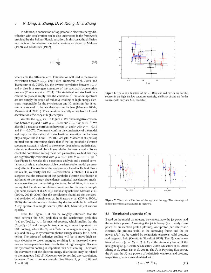
4.2 Magnetic field vs Doppler factor

We plot theδ as a function of theB in Figure 6. We find that anegative correlation betweenB andδ with the Pearson correlationcoefficientρ = −0.47 and the chance probabilityP = 0.0021 forour sample. In addition, we do a covariance analysis and a partialcorrelation analysis to exclude possible covariates (other model pa-rameters) effects. The results of the analyses are listed inTable 4.From the results, we verify that theB-δ correlation is reliable. Ac-cording to the SSC model, there are relationships betweenB andδ for a given source,Bδ ∝ [ν2

sy/νIC](1 + z) in Thomson regimeandB/δ ∝ [νsy/ν

2IC]/(1 + z) in the Klein-Nishina (KN) regime

(Tavecchio et al. 1998; Yan et al. 2014). Our result is in agreementwith the SSC model prediction and suggests thatB andδ are de-pendent on each other mainly in Thomson regime. Yan et al. (2014)explored the correlation betweenB andδ. Their sample consists of10 high-synchrotron peaked BL Lacs, 6 intermediate-synchrotronpeaked BL Lacs and 6 low-synchrotron peaked BL Lacs. Becausethe synchrotron peaks of their sources distribute in a largerange,the values of[ν2

sy/νIC] and the[νsy/ν2IC] are relatively scattered. It

causes they did not find any correlations betweenB andδ.

4.3 The particle acceleration and the radiative cooling

In the framework of statistical acceleration, Massaro et al. (2004a,2004b, 2006) showed that when the acceleration efficiency isin-versely proportional to the acceleration particles’s energy itself, theelectron energy distribution is curved into a log-parabolic shape,and its curvaturer is related to the fractional acceleration gainǫ,

r ∝1

log ǫ. (9)

r decreases whenǫ increases. Note that theEsy, IC = hνsy, IC scaleslike ǫ, whereh is Planck constant. Hence, according to this model,an inverse correlation betweenνsy, IC andr is expected.

15.0 15.5 16.0 16.50

2

4

6

8

10

0.0 0.2 0.4 0.6 0.8 1.00

2

4

6

8

10

12

14

5 10 15 20 25 30 35 400

2

4

6

8

10

12

14 16 18 20 22 24 260

4

8

12

16

20

N

log R [cm]

(a)

(d)

(b)

N

B [G]

(c)

N N

log Hz

Figure 4. Distributions of the radiation region radiusR (a), the magneticfield B (b), the beaming factorδ (c). (d) Distribution of the synchrotronradiation peak frequencyνsy (red solid line) and the inverse Compton scat-tering peak frequencyνIC (blue solid line).

14 15 16 17 18 1913

14

15

16

17

18

19

23 24 25 26

23

24

25

26

log

' sy [H

z]

log sy [Hz]

log

' IC [

Hz]

log IC [Hz]

Figure 5. The comparisons betweenνsy, νIC obtained by our andν′sy, ν′IC

obtained by Finke et al. (2013). The red lines arey = x. In here, we takethe average value for those sources that have the high and lowstate in oursample.

c© 0000 RAS, MNRAS000, 000–000


In addition, a connection of log-parabolic electron energydis-tribution with acceleration can be also understood in the frameworkprovided by the Fokker-Planck equation. In this case, the diffusionterm acts on the electron spectral curvature as given by Melrose(1969) and Kardashev (1962),

r ∝1

Dt, (10)

whereD is the diffusion term. This relation will lead to the inversecorrelation betweenνsy ,IC andr (see Tramacere et al. 2007a andTramacere et al. 2009). So, the inverse correlation betweenνsy ,IC

and r also is a strongest signature of the stochastic accelerationprocess (Tramacere et al. 2011). The statistical and stochastic ac-celeration process imply that the curvature of radiation spectrumare not simply the result of radiative cooling of high energyelec-trons, responsible for the synchrotron and IC emission, butis es-sentially related to the acceleration mechanism (Massaro 2004a,Massaro et al. 2011b). The curvature basically arises from aloss ofacceleration efficiency at high energies.

We plot theνsy, IC vs r in Figure 7. We find a negative correla-tion betweenνsy andr with ρ = −0.50 andP = 8.36× 10−4. Wealso find a negative correlation betweenνIC andr with ρ = −0.41andP = 0.0076. The results confirm the consistency of the modeland imply that the statistical or stochastic acceleration mechanismsplay a major role inFermi TeV BL Lacs jets. Massaro et al. (2004a)pointed out an interesting check that if the log-parabolic electronspectrum is actually related to the energy-dependence statistical ac-celeration, there should be a linear relation betweenr ands. So wecheck the correlation among these two parameters, we find that theyare significantly correlated withρ = 0.70 andP = 3.49 × 10−7

(see Figure 8). we also do a covariance analysis and a partialcorre-lation analysis to exclude possible covariates (other model parame-ters) effects. The results of the analyses are listed in Table 4. Fromthe results, we verify that ther-s correlation is reliable. The resultsuggests that the curvature of log-parabolic electron distribution isattributed to the energy-dependence statistical acceleration mech-anism working on the emitting electrons. In addition, it is worthnoting that the above correlations found are for the source sample(the same as Rani et al. (2011)), and distinguish from Massaro et al.(2004a, 2004b, 2006) that the correlations found are for thespec-tral evolution of a single source. In Massaro et al. (2004a, 2004b,2006), the correlations are obtained by dealing with the broadbandX-ray spectra of a single source (Mkn 421, Mkn 501) at variousepochs.

From the Figure 1, it can be roughly estimated that theratio between the SSC peak flux to the synchrotron peak flux(νfν)IC/(νfν)sy < 1 for most of sources, which implies that theUsyn/UB < 1 and the synchrotron cooling is more important thanSSC cooling, where theUB = B2/8π is the magnetic energy den-sity, and theUsyn is synchrotron photon energy density for IC scat-tering. The effect of radiative cooling will be to move high en-ergy electrons to lower energies, resulting in an increasedcurva-ture and a steepened electron distribution at high energies. Becausethe synchrotron cooling is important than SSC cooling. Therefore,the curvaturer of the electron energy distribution may be relatedto the magnetic fieldB. However, we do not find any correlationsbetweenB and r for our sample (See Figure 9,ρ = 0.09 andP = 0.54).

0.0 0.4 0.8 1.2

8

16

24

32

40

B [G]

Figure 6. The δ as a function of theB. Blue and red circles are for thesources in the high and low states, respectively, and black circles are for thesources with only one SED available.

22 24 2614 16 18 200.0

0.5

1.0

1.5

log IC [Hz]

r

log sy [Hz]

Figure 7. The r as a function of theνsy and theνIC. The meanings ofdifferent symbols are as same as Figure 6.

4.4 The physical properties of jet

Based on the model parameters, we can estimate the jet power andthe radiative power. Assuming the jet is heavy (i.e. mainly com-posed of an electron-proton plasma), one proton per relativisticelectron, the protons ’cold’ in the comoving frame, and the jetpower (Pjet) are be carried by relativistic electrons, cold protons,and magnetic field (Celotti & Ghisellini 2008). ThePjet can be es-timated withPjet = PB + Pe + Pp in the stationary frame of thehost galaxy (e.g., Celotti & Ghisellini 2008; Ghisellini etal. 2010;Zhang et al. 2012; Yan et al. 2014). ThePB is Poynting flux power,thePe and thePp are powers of relativistic electrons and protons,respectively, which are calculated with

Pi = πR2Γ2cUi (11)

c© 0000 RAS, MNRAS000, 000–000


0.0 0.2 0.4 0.6 0.8 1.0 1.2 1.40.5

1.0

1.5

2.0

2.5

3.0

s

r

Figure 8. Thes as a function of ther. The meanings of different symbolsare as same as Figure 6. The straight line is the best linear fitwith a slope,m = 1.19 ± 0.19 and constant,c = 0.98± 0.14 (y = mx+ c).

0.0 0.4 0.8 1.20.0

0.5

1.0

1.5

r

B [G]

Figure 9. Ther as a function of theB. The meanings of different symbolsare as same as Figure 6.

in the stationary frame of the host galaxy (Celotti & Fabian 1993;Celotti & Ghisellini 2008), where theΓ is the bulk Lorentz factor(we takeΓ = δ), and theUi (i = e, p, B) are the energy densitiesassociated with the emitting electronsUe, protonsUp, and magneticfieldUB in the comoving frame, respectively. TheUe is calculatedwith

Ue = mec2

∫γN(γ)dγ. (12)

The protons are considered ’cold’ in the comoving frame, theUp iscalculated with

Up = mpc2

∫N(γ)dγ (13)

by assuming one proton per emitting electron (see Celotti & Ghis-ellini 2008). TheUB is calculated with

UB = B2/8π (14)

The radiation power is estimated with the observed luminosity,

Pr = πR2Γ2cUr = L′ Γ2

4= L

Γ2

4δ4≈ L

1

4δ2, (15)

0.1 1 10 100 10002x1043

3x1043

4x1043

5x1043

6x1043

min=10 Pe

Pp

P [e

rg s

-1]

min

Figure 10. The Pe, Pp as a function of theγmin when the other physi-cal parameters take the average values of the sample (z = 0.163, R =

4.28E + 15, B = 0.45, δ = 24, N = 48, r = 0.79, s = 1.85, log γ0 =

3.5, log γmax = 6.2).

whereL is the total observed non-thermal luminosity in the Earth(L′ is in the comoving frame). Because the total observed non-thermal luminosity mainly comes from the jet, especially for TeVBL Lacs, so we takeL ∼ Lbol (bolometric luminosity of the jet).We calculateLbol in the band1010 − 1027 Hz based on our SEDfits, i.e.,Lbol = 4πd2L

∫ 1027Hz1010Hz Fobs(νobs)dνobs. The calculatedPe,

Pp,PB, andPr are listed in Table 3. From our SED modeling results(Figure 1), it can be seen that the GeV data at low energies canbefitted well. And the average spectral index between the X-rayandtheγ-ray of our calculated radiation spectrumsα′

Xγ = 1.12 is sim-ilar to the average observed value of the high peaked frequency BLLacsαXγ = 1.02 (Fan et al. 2012). Which implies the estimatedvalue ofγmin is reasonable. In addition, we give thePe andPp as afunction of theγmin in Figure 10 (Here, the other physical param-eters take the average values of the sample). It can be find that theγmin causes minor effect on the estimate of thePe andPp, espe-cially in γmin < 100. Therefore, we would like to believe that thepowers we derived here are creditable.

In Figure 11, we plot thePe, Pp, PB, Pjet as a function of thePr. A size relationPe ∼ Pp > Pr & PB can be found from Fig-ure 11. It should be pointed out that because the definitions of Ue,Up, UB are independent of each other, so the size relation ofPe,Pp, PB does not exist functional biases (Celotti & Ghisellini 2008).The Pe > PB suggests that the jets are particle dominated. ThePe ∼ Pp is consistent with Celotti & Ghisellini (2008) and meansthat the mean energy of relativistic electrons approachesmp/me

in TeV BL Lacs. ThePr & PB implies that Poynting flux can-not account for the radiation power. In fact, it can be found thatPr/Pe ∼ 0.01 − 1.5, which indicates that a large fraction of therelativistic electron power will be used to produce the observed ra-diation in some sources. So, as mentioned in Celotti & Ghisellini(2008), an additional reservoir of energy is needed to accelerateelectrons to high energies for those sources whose the relativisticelectron power is comparable to the emitted one.

It is generally believed that jet are driven by the accretionpro-cess and/or the spin of central black hole. Davis & Laor (2011)suggested that the black hole mass would be an essential factor forthe jet radiation efficiency and jet power. We investigate the rela-tion ofPjet to theM with a sub-sample of 18 sources in our sample.The black hole massM of these sources are collected from liter-

c© 0000 RAS, MNRAS000, 000–000


1043

1044

1045

1042

1043

1044

1045

1041

1042

1043

1044

1041 1042 1043 1044 10451043

1044

1045

1046

25Pr

5Pr

Pe [

erg

s-1]

Pr

25Pr

5Pr

Pr

Pp [

erg

s-1]

0.1Pr

0.3Pr

Pr

PB [

erg

s-1]

100Pr

10Pr

Pr

Pje

t [e

rg s

-1]

Pr [erg s-1]

Figure 11.ThePe, Pp, PB, Pjet as a function of thePr.

7.8 8.0 8.2 8.4 8.6 8.8 9.0 9.2

1043

1044

1045

Pje

t [er

g s-1

]

log M/Msun

Figure 12.ThePjet as a function of the black hole massM . The meaningsof different symbols are as same as Figure 6.

ature and reported (see Table 3), when more than one black holemasses are got, we use average value. ThePjet as a function of theM is shown in Figure 12. We do not find significant correlationsbetween the two parameters in high data (ρ = −0.56, P = 0.09)and in low state data (ρ = −0.48, P = 0.16). The result suggeststhat the jet power weakly depends on the black hole mass forFermiTeV BL Lac jets.

In Figure 13, we show that there is an anti-correlation be-tweenγpeak andPjet, i.e.,Pjet ∝ γ−1.02±0.19

peak with ρ = −0.647

andP = 4.9 × 10−6, whereγpeak is the electrons energy at thepeaks of the SED. For the log-parabolic electron energy distribu-tion here adopted, theγpeak = γ3p (the peak energy of the distribu-tion γ3N(γ)) and are calculated as given by Paggi et al. (2009b),

γpeak= γ3p = γp × 101/2r . (16)

104 105 1061043

1044

1045

Pje

t [er

g s-1

]

peak

Figure 13. ThePjet as a function of theγpeak. The meanings of differentsymbols are as same as Figure 6.

-0.8 -0.4 0.0 0.4-10 -5 0 5 10 150.0 0.7 1.4

0.4

0.8

1.2

1.6

2.0

2.4

[G]

lo

g F 1T

eV )

[Jy]

( log peak

)

Figure 14. The changes in the flux density at 1 TeV (F1TeV) as a functionof the changes inγpeak, δ, andB. The straight line is the best linear fit witha slope,m = 0.75± 0.27 and constant,c = 0.84± 0.16 (y = mx+ c).

whereγp = (∫γ2N(γ)dγ/

∫N(γ)dγ)1/2. The anti-correlation

betweenγpeakandPjet is consistent with the prediction of the blazarsequence (Fossati et al. 1998; Ghisellini et al. 1998; Celotti &Ghisellini (2008); Ghisellini & Tavecchio 2008) and is usually ex-plained as that the radiative cooling is stronger in more powerfulblazars.

4.5 The cause of flux variation

The SEDs of 14 sources in our sample are obtained the low and highTeV states. There are several possibilities that could be invoked toexplain the flux variation. 1) It is well known that the electron en-ergy distribution is influenced by several processes, such as accel-eration, escape and cooling. It is possible that the evolution of theelectron energy distribution leads to the flux variation. 2)Anotherreason to explain the flux variation is the change of the Dopplerboosting factor, presumably due to a change either the bulk veloc-ity or the viewing angle. Raiteri et al. (2010) found that only ge-ometrical (Doppler factor) changes are capable of explaining fluxvariation for BL Lacs. 3) In addition, the emission dissipation atdifferent location in the jet also may cause the flux variation. Since

c© 0000 RAS, MNRAS000, 000–000


the value of the magnetic fieldB is related to the location of thedissipation region. In this case, we expect to find that the change inB value is related to the flux variation.

we plot the changes in the flux density at 1 TeV (F1TeV) as afunction of the changes inγpeak, δ, B in Figure 14. We find a cor-relation between the changes in the flux density at 1 TeV and thechanges in theγpeak (ρ = 0.66, P = 0.02), but no statisticallycorrelations between the changes in the flux density at 1 TeV andthe changes inδ (ρ = −0.07, P = 0.83) andB (ρ = −0.20,P = 0.54) are found, which suggests the change/evolution of elec-tron energy distribution may be mainly responsible for the flux vari-ation. Our result is similar to Zhang et al. (2012) and supports theresearch results of single TeV BL Lac, e.g., Zheng et al. (2011a,2011b) investigated the rapid TeV flare in Mkn 501 and multi-wavelength variability in PKS 2155-304, their result showed thatthe flux variation is caused by the evolution of electron energy dis-tribution. Paggi et al. (2009b) investigated S5 0716+714, Mkn 501,Mkn 421 and found that the flares are directly related to accelera-tion of the emitting electrons.

5 CONCLUSIONS

In this work, we have modeled the quasi-simultaneous broadbandSEDs of 29Fermi TeV BL Lac objects by using a one-zone lep-tonic SSC model with the log-parabolic electron energy distribu-tion. We obtain the best-fit model parameters by MCMC samplingmethod. Then, we systematically investigate the physical proper-ties of Fermi TeV BL Lac jets. Our main results are the follow-ing: (i) There is a negative correlation betweenB and δ for oursource sample, which suggests thatB andδ are dependent on eachother mainly in Thomson regime. (ii) There are negative correla-tions betweenνsy andr, νIC and r for our source sample, whichconfirms the consistency of the model and is a signature of theenergy-dependence statistical acceleration or the stochastic accel-eration. We check the correlation betweenr ands, and find thatthey are significantly correlated. The result suggests thatthe curva-ture of log-parabolic electron energy distribution is attributed to theenergy-dependence statistical acceleration mechanism working onthe emitting electrons inFermi TeV BL Lacs. We do not find anycorrelations betweenB andr, which may be because the curvatureof the electron energy distribution is related to the particle accelera-tion rather than to the radiative cooling process. However,it shouldbe pointed out that because we use a "static" SSC code and do notconsider the evolution of the electron energy distribution, so theeffects of radiation cooling on the electron energy distribution arenot really addressed in here. (iii) By assuming one proton per rela-tivistic electron and the jet power are be carried by relativistic elec-trons, cold protons, magnetic field (Celotti & Ghisellini 2008). Wecalculate the jet power in different forms and the radiativepowerin the stationary frame of the host galaxy. We find a size relationPe ∼ Pp > Pr & PB. ThePe > PB suggests that the jets areparticle dominated inFermi TeV BL Lacs. ThePe ∼ Pp is consis-tent with Celotti & Ghisellini (2008) and means that the meanen-ergy of relativistic electrons approachesmp/me in Fermi TeV BLLacs. Then, we explore the correlation betweenPjet and black holemasses with a sub-sample of 18 sources in our sample. There arenot significant correlations whether in high or low state, which sug-gests that the jet power weakly depends on the black hole massforFermi TeV BL Lac jets. And we find thePjet ∝ γ−1.02±0.19

peak , whichis consistent with the prediction of the blazar sequence. (iv) At last,we explore the cause of flux variation. We only find a correlation

between the changes in the flux density at 1 TeV and the changesin theγpeak, which suggests the change/evolution of electron energydistribution may be mainly responsible for the flux variation in oursample.

ACKNOWLEDGMENTS

We sincerely thank anonymous referee for valuable commentsand suggestions. We are very grateful to the Science Foundationof Yunnan Province of China (2012FB140, 2010CD046). Thiswork is supported by the National Nature Science FoundationofChina (11063004, 11163007, U1231203), and the High-EnergyAstrophysics Science and Technology Innovation Team of YunnanHigher School and Yunnan Gravitation Theory Innovation Team(2011c1). This research has made use of the NASA/IPAC Extra-galactic Database (NED), that is operated by Jet PropulsionLabo-ratory, California Institute of Technology, under contract with theNational Aeronautics and Space Administration.

REFERENCES

Abdo, A. A., et al. 2009, ApJ, 700, 597Abdo, A. A., et al. 2010a, ApJ, 716, 30Abdo, A. A., Ackermann, M., Ajello, M., et al. 2010b, ApJ, 708,1310

Abdo, A. A., et al. 2011a, ApJ, 736, 131Abdo, A. A., Ackermann, M., Ajello, M., et al. 2011b, ApJ, 726,43

Acciari, V. A., Aliu, E., Beilicke, M., et al. 2008, ApJ, 684,73Acciari, V. A., Aliu, E., Aune, T., et al. 2009a, ApJ, 707, 612Acciari, V., Aliu, E., Arlen, T., et al. 2009b, ApJ, 690, 126Acciari, V. A., Aliu, E., Arlen, T., et al. 2010a, ApJ, 708, 100Acciari, V. A., Aliu, E., Arlen, T., et al. 2010b, ApJ, 715, 49Acciari, V. A., Aliu, E., Arlen, T., et al. 2011, ApJ, 738, 169Ackermann, M., Ajello, M., Allafort, A., et al. 2011, ApJ, 743,171

Aharonian, F., Akhperjanian, A. G., Bazer-Bachi, A. R., et al.2007, A&A, 470, 475

Aharonian, F., Akhperjanian, A. G., Barres de Almeida, U., et al.2008, A&A, 481, 103

Aharonian, F., Akhperjanian, A. G., Anton, G., et al. 2009a,A&A,502, 749

Aharonian, F., Akhperjanian, A. G., Anton, G., et al. 2009b,ApJ,696, 150

Aharonian, F. A., Kelner, S. R., Prosekin, A. Yu. 2010, PhRvD,82, 3002

Albert, J., Aliu, E., Anderhub, H., et al. 2007a, ApJ, 662, 89Albert, J., Aliu, E., Anderhub, H., et al. 2007b, ApJ, 666, 17Albert, J., Aliu, E., Anderhub, H., et al. 2007c, ApJ, 667, 21Aleksic, J., et al. 2012a, A&A, 544, 142Aleksic, J., et al. 2012b, A&A, 539, 118Aleksic, J., et al. 2014a, A&A, 567, 135Aleksic, J., et al. 2014b, A&A, 572, 121Aliu E., et al. 2012, ApJ, 755, 118Anderhub, H., Antonelli, L. A., Antoranz, P., et al. 2009a, ApJ,705, 1624

Anderhub, H., Antonelli, L. A., Antoranz, P., et al. 2009b, ApJ,704, 129

Böttcher, M. 2007 Ap&SS, 309, 95

c© 0000 RAS, MNRAS000, 000–000


Blazejowski, M., Blaylock, G., Bond, I. H., et al. 2005, ApJ,630,130

Celotti, A., & Fabian, A. C. 1993, MNRAS, 264, 228Celotti, A., & Ghisellini, G. 2008, MNRAS, 385, 283Davis, S. W., & Laor, A. 2011, ApJ, 728, 98Dermer, C. D., & Schlickeiser, R. 1993, ApJ, 416,458Dermer, C. D. 1995, ApJ, 446, 63Dermer, C. D., Schlickeiser, R. 2002, ApJ, 575, 667Dermer, C. D., Finke, J. D., Krug, H., & Bö ttcher, M. 2009, ApJ,692, 32

Dermer, C. D., Murase, K., Takami, H. 2012, ApJ, 755, 147Dermer, C. D., Yan, D. H., Zhang, L., Finke, J. D., Lott, B. 2015,ApJ, 809, 174

Dwek, E., & Krennrich, F., 2005, ApJ, 618, 657Falomo, R., Pian, E., Treves, A. 2014 A&ARv 22, 73Fan, J. H., Yang, J. H., Yuan, Y. H., Wang, J., Gao, Y. 2012, ApJ,761, 125

Finke, J. D. 2013, ApJ, 763, 134Foreman-Mackey, D., Hogg, D. W., Lang, D., & Goodman, J.2013, PASP, 125, 306.

Fossati, G., Maraschi, L., Celotti, A., Comastri, A., Ghisellini, G.1998 MNRAS, 299, 433

Ghisellini, G., Guilbert, P. W., & Svensson, R. 1988, ApJ, 334, 5Ghisellini, G., Celotti, A., Fossati, G., Maraschi, L., Comastri, A.1998, MNRAS, 301, 451

Ghisellini, G., & Tavecchio, F. 2008, MNRAS, 387, 1669Ghisellini, G., Tavecchio, F., Ghirlanda, G. 2009, MNRAS, 399,2041

Ghisellini, G., Tavecchio, F., Foschini, L., et al. 2010, MNRAS,402, 497

Ghisellini, G., Tavecchio, F., Foschini, L., Ghirlanda, G.2011,MNRAS, 414, 2674

Giommi, P., et al. 2012, A&A, 541, 160Goodman, J., Weare, J., 2010. Commun. Appl. Math. Comput.Sci., 5, 65

HESS Collaboration, Acero, F., Aharonian, F., et al. 2010, A&A,511, 52

HESS Collaboration, Abramowski, A., Acero, F., et al. 2010a,A&A, 516, A56

Jones, F. C. 1968, PhRv, 167, 1159Kang, S. J., Zheng, Y. G., Wu, Q. W., Chen, L. 2016, MNRAS,461, 1862

Kardashev, N. S. 1962, SvA, 6, 317Kataoka, J., Mattox, J. R., Quinn, J., et al. 1999, ApJ, 514, 138Kaufmann, S., Hauser, M., Kosack, K., et al. 2010, BAAS, 42,709

Krawczynski, H., Hughes, S. B., Horan, D., et al. 2004, ApJ, 601,151

Lähteenmaki, A., Valtaoja, E. 2003, ApJ, 590, 95Lister, M. L., Aller, M. F., et al. 2013, AJ, 146, 120Lister, M. L., Aller, M. F., et al. 2016, AJ, 152, 12Machalski, J. & Jamrozy, M. 2006, A&A, 454, 95Massaro, F. & Grindlay, J. E. 2011, ApJ, 727, 1Massaro, E., Perri, M., Giommi, P., Nesci, R. 2004a, A&A, 413,489

Massaro, E., Perri, M., Giommi, P., Nesci, R., Verreccia, F.2004b,A&A, 422, 103

Massaro, E., Tramacere, A., Perri, M., Giommi, P., Tosti, G.2006,A&A, 448, 861

Massaro, F., Paggi, A., Elvis, M., Cavaliere, A. 2011a, ApJ,739,73

Massaro, F., Paggi, A., Cavaliere, A. 2011b, ApJ, 742, 32

Massaro, F., Paggi, A., Errando, M., D’Abrusco, R., Masetti, N.,Tosti, G., Funk, S. 2013, ApJS, 207, 16

Massaro, F., Masetti, N., D’Abrusco, R., Paggi, A., Funk, S.2014,AJ, 148, 66

Massaro, F., Thompson, D. J., Ferrara, E. C. 2016, A&ARv, 24,2Melrose, D. B. 1969, Ap&ss, 5, 131Paggi, A., Massaro, F., Vittorini, V., Cavaliere, A., D’Ammando,F., Vagnetti, F., Tavani, M. 2009a, A&A, 504, 821

Paggi, A., Cavaliere, A., Vittorini, V., Tavani, M. 2009b, A& A,508, 31

Prandini E., Bonnoli G., Tavecchio F. 2012, A&A, 543, 111Rügamergamer, S., Angelakis, E., Bastieri, D., et al. 2011,arXiv1109.6808R

Rüger, M., Spanier, F., & Mannheim, K. 2010, MNRAS, 401, 973Raiteri, C. M., et al. 2010, A&A, 524, 43Rani, B., Gupta, A. C., Bachev, R., et al. 2011, MNRAS, 417,1881

Reimer, A., Costamante, L., Madejski, G., Reimer, O., & Dorner,D. 2008, ApJ,682, 775

Savolainen, T., Homan D. C., Hovatta, T., et al., 2010, A& A, 512,24

Sikora, M., Begelman, M. C., & Rees, M. J. 1994, ApJ, 421, 153Singha, K. K., Yadav, K. K., et al. New Astronomy, 36, 1Tagliaferri, G., Foschini, L., Ghisellini, G., et al. 2008,ApJ, 679,1029

Tavecchio, F., Maraschi, L., Ghisellini, G. 1998, ApJ, 509,608Tavecchio, F., Maraschi, L., Sambruna, R. M., Urry, C. M. 2000,ApJ, 544, 23

Tavecchio, F., Maraschi, L., Pian, E., et al. 2001, ApJ, 554,725Tavecchio, F., Ghisellini, G., Ghirlanda, G., Foschini, L., &Maraschi, L. 2010, MNRAS, 401, 1570

Tramacere, A., Massaro, F., Cavaliere, A. 2007a, A&A, 466, 521Tramacere, A., Giommi, P., Massaro, E., et al. 2007b, A&A, 467,501

Tramacere, A., Giommi, P., Perri, M., Verrecchia, F., Tosti, G.2009, A& A, 501, 879

Tramacere, A., Massaro, E., Taylor, A. M. 2011, ApJ, 739, 66Urry, C. M. & Padovani, P. 1995, PASP, 107, 803Wolter, A., Beckmann, V., Ghisellini, G., Tavecchio, F., &Maraschi, L. 2008, ASPC, 386, 302

Yan, D. H., Zeng, H. D., Zhang, L., 2014, MNRAS, 439, 2933Zabalza, V. 2015, in Proc. of Interna-tional Cosmic Ray Conference 2015,http://adsabs.harvard.edu/abs/2015arXiv150903319Z

Zhang, J., Liang, E. W., Zhang, S. N., Bai, J. M. 2012 ApJ, 752,157

Zheng, Y. G., Zhang, L. 2011, ApJ, 728, 105Zheng, Y. G., Zhang, L., Zhang, X., Ma, H. J. 2011, JApA, 32,327

c© 0000 RAS, MNRAS000, 000–000

http://adsabs.harvard.edu/abs/2015arXiv150903319Z


Table 1.The time of quasi-simultaneous observation, the observed telescopes, and the references for each source

Name State Time The observed telescopes Ref(1) (2) (3) (4) (5)

1ES 1101-232 H 2006-May Suzaku, H.E.S.S. Reimer et al. 2008L 2004-Jun to 2005-Mar XMM-Newton,RXTE, H.E.S.S. Aharonian et al. 2007

Mkn421 H 2003-Feb to 2004-Jun FLWO,RXTE, Whipple Blazejowski et al. 2005L 2009-Jan to 2009-Jun Swift-UVOT, Swift-XRT, Swift-BAT, Fermi-LAT, MAGIC Abdo et al. 2011a

Mkn501 H 1997-Apr BeppoSAX, CAT Tavecchio et al. 2001L 2006-Jul KVA,Suzaku, MAGIC Anderhub et al. 2009a

1ES 1959+650 H 2002-May to 2002-Jun Boltwood Observatory, Abastumani Observatory,RXTE, HEGRA Krawczynski et al. 2004L 2006-May Swift-UVOT, Suzaku, MAGIC Tagliaferri et al. 2008

PKS 2005-489 H 2009-May to 2009 July Swift-UVOT, RXTE, Swift-XRT, H.E.S.S. Kaufmann et al. 2010L 2004-Oct XMM-Newton H.E.S.S. Collaboration et al. 2010a

PKS 2155-304 H 2006-Jul Bronberg Observatory,RXTE, Chandra, H.E.S.S. Aharonian et al. 2009aL 2008-Aug to 2008-Sep ATOM,RXTE, H.E.S.S. Aharonian et al. 2009b

1ES 2344+514 H 2007-Dec Swift-UVOT, Swift-XRT, VERITAS Acciari et al. 2011L 2005-Apr to 2006-Jan KVA,Swift-XRT, MAGIC Albert et al. 2007a; Tramacere et al. 2007b

W Comae H 2008-Jun Swift-UVOT, Swift-XRT, VERITAS Acciari et al. 2009L 2008-May (low state) AAVSO,Swift-UVOT, Swift-XRT, Fermi-LAT∗ , VERITAS Acciari et al. 2008; Tavecchio et al. 2010

S5 0716+714 H 2008-Apr KVA,Swift-XRT, MAGIC Anderhub et al. 2009bL 2008-Nov Swift-UVOT, Swift-XRT Tavecchio et al. 2010

BL Lacertae H 2005-Aug to 2005-Dec (low state) KVA, EGRET∗ , MAGIC Albert et al. 2007bL 2008-Aug to 2008-Oct Effelsberg Observatory,Swift-UVOT, GASP-WEBT Collaboration,Swift-XRT, Fermi-LAT Abdo et al. 2010a

1ES 1011+496 H 2008-May (high state) Swift-UVOT, Swift-XRT, MAGIC∗ Albert et al. 2007c; Tavecchio et al. 2010L 2008-Aug to 2008-Oct OVRO,Swift-UVOT, Swift-XRT, Fermi-LAT Abdo et al. 2010a

MAGIC J2001+435 H 2010-Jul Swift-UVOT, Swift-XRT, MAGIC Aleksic et al. 2014bL 2010-Jul to 2010-Sep (low state) OVRO,Swift-UVOT, Swift-XRT, Fermi-LAT Aleksic et al. 2014b

Mkn180 2008-May (low state) Swift-UVOT, Swift-XRT, MAGIC∗ Rügamer et al. 20113C 66A 2008-Oct MDM,Swift-UVOT, Swift-XRT, Fermi-LAT, VERITAS Abdo et al. 2011b

PKS 1424+240 2009-Feb to 2009-Jun MDM,Swift-UVOT, Swift-XRT, Fermi-LAT, VERITAS Acciari et al. 2010a1ES 1215+303 2011-Jan to 2011-Feb Metsähovi, KVA,Swift-UVOT, Swift-XRT, Fermi-LAT, MAGIC Aleksic et al. 2012a

1RXS J003334.6-192130 2008-May to 2008-Nov Swift-UVOT, Swift-XRT, Fermi-LAT Abdo et al. 2010aRGB J0152+017 2007-Nov RXTE, Swift-XRT, H.E.S.S. Aharonian et al. 20081ES 0414+009 2010-Jul to 2011-Feb MDM,Swift-XRT, Fermi-LAT, VERITAS Aliu et al. 2012PKS 0447-439 2009-Nov to 2010 Jan Swift-UVOT, Swift-XRT, Fermi-LAT, H.E.S.S. Prandini et al. 2012

RGB J0710+591 2008-Dec to 2009-Mar MDM,Swift-UVOT, Swift-XRT, VERITAS Acciari et al. 2010b1ES 0806+524 2007-Nov to 2008-Apr Swift-UVOT, Swift-XRT, VERITAS Acciari et al. 2009b

MS 1221.8+2452 2013-Mar to 2013-Apr (low state) OVRO,Swift-UVOT, Swift-XRT, MAGIC∗ , VERITAS∗ Singh et al. 2014H 1426+428 low state BeppoSAX∗ , INTEGRAL∗ , CAT∗ , HEGRA∗ Wolter et al. 2008

PG 1553+113 2006-Apr to 2006 Jul (low state) Suzaku, Fermi-LAT∗ , MAGIC, H.E.S.S. Abdo et al. 2010bB3 2247+381 2010-Sep to 2010-Oct (low state) Plank∗, KVA, Swift-XRT, Fermi-LAT∗ , MAGIC Aleksic et al. 2012b1ES 1741+196 2010-Feb to 2010-Apr ATCA, Plank,Swift-UVOT, Swift-XRT, Fermi-LAT Giommi et al. 20121ES 1218+30.4 2005-Jan to 2005-March KVA,Swift-XRT, MAGIC Rüger et al. 2010

H 2356-309 2005-June XMM-Newton, H.E.S.S. H.E.S.S. Collaboration et al. 2010b

Notes.Column (2) is the state of each source in TeV band. "H" indicating "high state" and "L" indicating "low state". Column (3) is the time ofquasi-simultaneous observation, the content in the bracket is the state of the source in the time of quasi-simultaneousobservation. In here, H 1426+428 has noquasi-simultaneous observation, we use its SED data that itis in low state. Column (4) is the observed telescopes, the superscript ’∗’ represents that the dataof observed telescope are not in the time of quasi-simultaneous observation, but the state of these data consistent withthat in the time of quasi-simultaneousobservation. Column (5) is the references of the quasi-simultaneous broadband SEDs.

c© 0000 RAS, MNRAS000, 000–000


Table 2.The best-fit model parameters and the flux density at 1 TeV

Name State z R (cm) B (G) δ r s N log γ0 log γmax F1TeV (Jy)(1) (2) (3) (4) (5) (6) (7) (8) (9) (10) (11) (12)

1ES 1101-232 H 0.186 4.47E+15 0.20+0.12−0.08

37+4

−30.39+0.13

−0.121.23+0.21

−0.2378+3

−32.4+0.2

−0.36.2+0.2

−0.41.1E-15

L 3.16E+15 0.97+0.09−0.10

23+4

−30.74+0.10

−0.121.84+0.16

−0.185 +2

−43.9+0.2

−0.26.5+0.3

−0.23.8E-16

Mkn421 H 0.030021 2.19E+15 0.53+0.17−0.12

21+3

−10.65+0.11

−0.131.61+0.14

−0.1340+3

−33.8+0.3

−0.26.8+0.6

−0.71.6E-13

L 3.98E+15 0.32+0.10−0.10

29+2

−20.90+0.02

−0.081.85+0.28

−0.212 +4

−14.0+0.2

−0.26.7+0.5

−0.62.9E-14

Mkn501 H 0.033663 7.94E+14 0.31+0.18−0.17

25+1

−10.30+0.14

−0.162.01+0.21

−0.2242+2

−55.0+0.3

−0.46.7+0.7

−0.61.4E-13

L 1.58E+15 0.34+0.16−0.19

23+4

−50.56+0.12

−0.141.32+0.20

−0.2050+5

−33.2+0.1

−0.16.0+0.7

−0.63.9E-15

1ES 1959+650 H 0.047 1.26E+15 0.40+0.16−0.13

30+2

−30.80+0.10

−0.121.99+0.18

−0.2435+3

−24.3+0.3

−0.36.3+0.4

−0.45.1E-14

L 3.16E+15 0.95+0.15−0.19

16+2

−30.70+0.04

−0.041.95+0.12

−0.116 +1

−34.0+0.1

−0.26.3+0.2

−0.12.0E-15

PKS 2005-489 H 0.071 2.09E+16 0.12+0.07−0.05

38+2

−20.30+0.12

−0.131.10+0.24

−0.2810+2

−41.5+0.2

−0.26.3+0.2

−0.22.6E-15

L 2.45E+15 0.15+0.06−0.04

38+5

−21.21+0.11

−0.092.63+0.26

−0.2897+7

−53.8+0.2

−0.26.5+0.2

−0.31.4E-16

PKS 2155-304 H 0.116 5.25E+15 0.32+0.12−0.17

23+4

−20.93+0.06

−0.052.08+0.18

−0.1455+5

−44.0+0.4

−0.35.8+0.6

−0.42.9E-13

L 3.16E+15 0.74+0.17−0.11

21+3

−20.84+0.08

−0.052.09+0.10

−0.1134+3

−23.8+0.2

−0.25.9+0.5

−0.68.4E-15

1ES 2344+514 H 0.044 1.00E+15 0.35+0.08−0.11

17+3

−50.62+0.05

−0.031.92+0.25

−0.2342+4

−24.4+0.2

−0.25.9+0.6

−0.71.6E-14

L 1.02E+15 0.28+0.13−0.16

27+3

−50.79+0.08

−0.101.83+0.24

−0.2258+4

−43.7+0.3

−0.35.5+0.4

−0.21.7E-15

W Comae H 0.102 4.47E+15 0.11+0.06−0.03

32+3

−20.83+0.06

−0.091.45+0.16

−0.2080+3

−43.3+0.3

−0.46.4+0.5

−0.36.6E-15

L 5.25E+15 0.35+0.16−0.17

18+1

−30.84+0.06

−0.061.54+0.19

−0.2960+3

−43.2+0.3

−0.36.4+0.5

−0.31.7E-15

S5 0716+714 H 0.3 2.00E+16 0.23+0.12−0.09

26+1

−10.92+0.03

−0.032.20+0.28

−0.3520+3

−33.6+0.2

−0.25.8+0.5

−0.34.7E-16

L 2.00E+16 0.93+0.16−0.18

18+3

−20.80+0.04

−0.032.20+0.36

−0.35100+5

−43.0+0.2

−0.25.9+0.3

−0.23.2E-18

BL Lacertae H 0.0686 6.31E+15 0.11+0.04−0.02

24+1

−30.91+0.10

−0.102.12+0.13

−0.2150+3

−33.6+0.2

−0.25.9+0.4

−0.61.9E-16

L 9.77E+15 0.32+0.16−0.17

24+4

−50.76+0.14

−0.131.98+0.22

−0.1785+4

−42.9+0.3

−0.35.9+0.2

−0.31.4E-17

1ES 1011+496 H 0.212 3.24E+15 0.96+0.11−0.12

28+2

−20.85+0.03

−0.032.30+0.26

−0.2415+3

−44.1+0.2

−0.26.6+0.5

−0.12.6E-15

L 5.01E+15 0.89+0.09−0.10

17+4

−50.78+0.03

−0.061.87+0.30

−0.2644+2

−23.5+0.1

−0.26.1+0.4

−0.62.4E-16

MAGIC J2001+435 H 0.18 5.25E+15 0.18+0.06−0.03

25+3

−20.98+0.12

−0.202.05+0.37

−0.3175+3

−53.7+0.2

−0.25.9+0.5

−0.72.9E-16

L 1.26E+16 0.14+0.04−0.02

27+2

−21.01+0.05

−0.062.20+0.19

−0.2045+4

−53.4+0.2

−0.26.6+0.2

−0.31.0E-17

Mkn180 0.045278 1.29E+15 0.33+0.05−0.04

22+4

−40.65+0.16

−0.131.63+0.34

−0.3250+3

−43.5+0.2

−0.36.1+0.8

−0.7

3C 66A 0.444 1.23E+16 0.16+0.08−0.05

30+4

−30.90+0.10

−0.112.05+0.18

−0.17100+5

−43.5+0.3

−0.26.1+0.4

−0.3

PKS 1424+240 0.16 5.01E+15 0.38+0.18−0.11

27+4

−51.10+0.14

−0.162.70+0.28

−0.1245+5

−43.8+0.2

−0.25.9+0.5

−0.3

1ES 1215+303 0.13 1.38E+16 0.09+0.03−0.02

27+4

−30.53+0.12

−0.131.35+0.19

−0.1690+2

−22.5+0.3

−0.36.3+0.3

−0.4

1RXS J003334.6-192130 0.61 1.00E+16 0.65+0.13−0.18

21+3

−40.55+0.14

−0.111.40+0.20

−0.2085+3

−32.7+0.2

−0.36.6+0.6

−0.8

RGB J0152+017 0.08 2.51E+15 0.20+0.15−0.10

20+3

−30.36+0.12

−0.191.70+0.26

−0.2280+4

−33.2+0.2

−0.36.6+0.5

−0.4

1ES 0414+009 0.287 7.76E+15 0.62+0.09−0.09

23+5

−40.59+0.09

−0.091.72+0.31

−0.3010+1

−43.3+0.2

−0.16.6+0.3

−0.5

PKS 0447-439 0.107 7.59E+15 0.52+0.13−0.15

14+3

−30.82+0.16

−0.141.51+0.25

−0.2630+6

−43.3+0.4

−0.25.9+0.3

−0.2

RGB J0710+591 0.125 1.58E+15 0.72+0.14−0.13

28+4

−30.62+0.04

−0.042.40+0.20

−0.2220+3

−24.3+0.4

−0.26.0+0.3

−0.1

1ES 0806+524 0.138 2.82E+15 0.57+0.10−0.11

20+2

−30.90+0.11

−0.141.68+0.15

−0.2037+4

−33.5+0.2

−0.26.4+0.2

−0.2

MS 1221.8+2452 0.183648 6.31E+15 0.29+0.16−0.10

20+3

−10.52+0.10

−0.101.78+0.19

−0.1760+2

−33.4+0.2

−0.16.5+0.4

−0.2

H 1426+428 0.129139 2.51E+15 0.11+0.08−0.04

32+3

−30.36+0.11

−0.101.20+0.30

−0.3390+5

−42.8+0.4

−0.46.0+0.4

−0.3

PG 1553+113 0.36 3.89E+15 0.96+0.18−0.19

27+2

−40.98+0.10

−0.092.61+0.19

−0.1813+3

−24.3+0.4

−0.36.7+0.5

−0.4

B3 2247+381 0.1187 3.98E+15 0.75+0.15−0.19

17+4

−30.84+0.10

−0.111.81+0.34

−0.345 +2

−23.7+0.1

−0.26.7+0.6

−0.5

1ES 1741+196 0.084 3.98E+16 0.65+0.15−0.15

8 +4

−40.31+0.06

−0.051.60+0.13

−0.1623+2

−22.2+0.2

−0.16.1+0.5

−0.5

1ES 1218+30.4 0.183648 1.45E+15 0.65+0.12−0.18

31+3

−51.06+0.13

−0.122.25+0.19

−0.1752+5

−24.0+0.2

−0.26.0+0.3

−0.6

H 2356-309 0.165388 2.29E+15 0.59+0.13−0.17

18+2

−40.57+0.10

−0.111.42+0.14

−0.1149+4

−43.3+0.2

−0.26.2+0.5

−0.4

Notes.Column (12) is the observed or extrapolated flux density at 1 TeV.

c© 0000 RAS, MNRAS000, 000–000


Table 3.The jet powers in the different forms (Pe, Pp, PB), the radiative powers (Pr), and the black hold masses

Name State Pe (erg s−1) Pp (erg s−1) PB (erg s−1) Pr (erg s−1) log(MBH/M⊙) Ref(1) (2) (3) (4) (5) (6) (7) (8)

1ES 1101-232 H 9.88E+43 3.03E+44 4.09E+42 3.89E+42L 9.55E+42 3.75E+42 1.87E+43 1.06E+43

Mkn421 H 3.48E+43 1.15E+43 2.13E+42 2.26E+43 8.5, 8.29, 8.22, 7.6 Sb12, W02, C12, X04L 1.17E+43 3.78E+42 5.11E+42 1.65E+42

Mkn501 H 1.77E+43 2.35E+42 1.42E+41 8.30E+42 9, 9.21, 8.3 Sb12, W02, X04L 1.18E+43 9.41E+42 5.76E+41 8.34E+41

1ES 1959+650 H 3.27E+43 6.83E+42 8.27E+41 7.66E+42 8.1 Z12L 5.65E+42 2.17E+42 8.66E+42 6.85E+42

PKS 2005-489 H 1.09E+44 9.01E+44 3.40E+43 3.40E+42 8.1 X04L 1.50E+44 1.20E+44 7.34E+41 1.79E+42

PKS 2155-304 H 3.16E+44 1.13E+44 5.59E+42 2.91E+44 8.7 Z12L 3.45E+43 2.15E+43 9.17E+42 1.86E+43

1ES 2344+514 H 1.08E+43 1.73E+42 1.33E+41 2.54E+42 8.8 W02L 1.18E+43 6.39E+42 2.28E+41 3.42E+41

W Comae H 2.70E+44 2.32E+44 9.26E+41 6.51E+42 8 X04L 6.89E+43 7.87E+43 4.25E+42 9.07E+42

S5 0716+714 H 7.31E+44 7.39E+44 5.17E+43 2.08E+44 8.1, 8.1 C12, X04L 3.67E+44 1.83E+45 4.18E+44 2.15E+44

BL Lacertae H 1.65E+44 1.66E+44 1.07E+42 3.09E+42 8.7, 8.23, 7.7 Sb12, W02, X04L 1.43E+44 6.79E+44 2.16E+43 4.58E+42

1ES 1011+496 H 3.90E+43 1.68E+43 2.73E+43 4.26E+43 8.3 Z12L 4.95E+43 4.63E+43 2.23E+43 4.86E+43

MAGIC J2001+435 H 2.52E+44 1.84E+44 1.99E+42 2.02E+43L 4.89E+44 7.58E+44 8.10E+42 1.33E+43

Mkn180 1.05E+44 1.36E+44 5.01E+42 2.53E+43 8.21 W023C 66A 1.76E+45 1.93E+45 1.31E+43 3.16E+44 8.6, 8 C12, X04

PKS 1424+240 1.20E+44 1.17E+44 9.91E+42 1.33E+431ES 1215+303 4.40E+44 1.78E+45 4.22E+42 5.31E+42 8.12 W02

1RXS J003334.6-192130 1.76E+44 5.14E+44 6.65E+43 1.01E+44RGB J0152+017 1.40E+43 2.90E+43 3.78E+41 5.79E+411ES 0414+009 3.33E+43 4.59E+43 4.65E+43 1.64E+43PKS 0447-439 4.87E+43 4.87E+43 1.16E+43 2.21E+43

RGB J0710+591 1.00E+43 5.50E+42 3.77E+42 3.12E+42 8.26 W021ES 0806+524 2.18E+43 1.59E+43 3.72E+42 4.47E+42 8.9 Z12

MS 1221.8+2452 7.71E+42 5.77E+42 3.13E+41 3.17E+41H 1426+428 7.55E+43 8.24E+43 2.93E+41 2.46E+42 9.13 W02

PG 1553+113 5.72E+43 2.03E+43 3.81E+43 8.57E+43B3 2247+381 6.15E+42 3.29E+42 9.79E+42 3.18E+421ES 1741+196 3.46E+43 3.47E+44 1.68E+44 4.54E+431ES 1218+30.4 3.59E+43 1.49E+43 3.20E+42 8.61E+42 8.58 W02

H 2356-309 1.51E+43 1.18E+43 2.22E+42 4.99E+42 8.6 W02

Notes.Column (8) is the references of black hole masses. C12: Chai et al. (2012); Sb12: Shaw et al. (2012); W02: Woo & Urry (2002);X04: Xie et al. (1991,2004); Z12: Zhang et al. (2012).

Table 4.The results of covariance analysis and partial correlationanalysis forB-δ correlation andr-s correlation

B-δ correlation

covariatea R N r s γ0 γmax

Chance probability of covariance analysis(Pcov)b 0.06 0.53 0.10 0.35 0.08 0.76Pearson coefficient of partial correlation analysis (ρpar)

c -0.48 -0.42 -0.49 -0.52 -0.47 -0.48Chance probability of partial correlation analysis (Ppar)

d 0.002 0.006 0.001 0.001 0.002 0.001

r-s correlation

covariate B δ R N γ0 γmax

Chance probability of covariance analysis (Pcov) 0.19 0.29 0.18 0.43 0.42 0.42Pearson coefficient of partial correlation analysis (ρpar) 0.73 0.69 0.70 0.70 0.59 0.69Chance probability of partial correlation analysis (Ppar) < 0.001 < 0.001 < 0.001 < 0.001 < 0.001 < 0.001

Notes.a. Possible covariate in correlation analysis (B-δ correlation andr-s correlation). b. The results of covariance analysis. Null hypothesis: there existsthe influence of covariate (i.e., If the chance probability of covariance analysisPcov < 0.05, there exists the influence of covariate). c. The Pearson correlationcoefficient excluding the influence of covariate. d. The chance probability of correlation excluding the influence of covariate. If the chance probability ofpartial correlation analysisPpar < 0.05, there exists the correlation between dependent variable and independent variable excluding the influence of covariate(Machalski & Jamrozy 2006).

c© 0000 RAS, MNRAS000, 000–000

the physical properties of fermi tev bl lac objects jets · we investigate the physical properties...

Documents