HAL Id: hal-00583163https://hal.archives-ouvertes.fr/hal-00583163

Submitted on 5 Apr 2011

HAL is a multi-disciplinary open accessarchive for the deposit and dissemination of sci-entific research documents, whether they are pub-lished or not. The documents may come fromteaching and research institutions in France orabroad, or from public or private research centers.

L’archive ouverte pluridisciplinaire HAL, estdestinée au dépôt et à la diffusion de documentsscientifiques de niveau recherche, publiés ou non,émanant des établissements d’enseignement et derecherche français ou étrangers, des laboratoirespublics ou privés.

The impact of interregional and intraregionaltransportation costs on industrial location and efficient

transport policiesPaul Chiambaretto, André de Palma, Stef Proost

To cite this version:Paul Chiambaretto, André de Palma, Stef Proost. The impact of interregional and intraregionaltransportation costs on industrial location and efficient transport policies. 2011. �hal-00583163�

THE IMPACT OF INTERREGIONAL AND INTRAREGIONAL TRANSPORTATION COSTS

ON INDUSTRIAL LOCATION AND EFFICIENT TRANSPORT POLICIES

Paul CHIAMBARETTO André DE PALMA

Stef PROOST

March 2011

Cahier n° 2011-09

ECOLE POLYTECHNIQUE CENTRE NATIONAL DE LA RECHERCHE SCIENTIFIQUE

DEPARTEMENT D'ECONOMIE Route de Saclay

91128 PALAISEAU CEDEX (33) 1 69333033

http://www.economie.polytechnique.edu/ mailto:chantal.poujouly@polytechnique.edu

1

The impact of interregional and intraregional transportation costs

on industrial location and efficient transport policies

March 2011

Paul CHIAMBARETTO1 (corresponding author)

PREG-CRG, Ecole Polytechnique, 32 bd Victor, 75015 Paris, France

paul.chiambaretto@polytechnique.edu

André DE PALMA2

ENS Cachan, 61 av du Pr. Wilson, 94235 Cachan, France

Centre d’Economie de la Sorbonne, University Paris I, Paris, France

And Ecole Polytechnique, Palaiseau, France

andre.depalma@ens-cachan.fr

Stef PROOST2

Center for Economic Studies, KU Leuven, Naamsestraat 69, 3000 Leuven, Belgium

stef.proost@econ.kuleuven.be

Abstract: Almost all models of the (New) Economic Geography have focused on

interregional transportation costs to understand industrial location, considering regions as dots

without intraregional transportation costs. We introduce a distinction between interregional

and intraregional transportation costs. This allows assessing more precisely the effects of

different types of transport policies. Focusing on two regions (a core and a periphery), we

show that improving the quality of the interregional infrastructure, or of the intraregional

infrastructure in the core region, leads to an increased concentration of activity in the core

region. However, if we reduce intraregional transportation costs in the periphery, some firms

transfer from the core to the periphery. From an efficiency point of view, we observe that, in

absence of regulation, the concentration of firms is too high in the center. We show what set

of policies improves the equilibrium.

JEL Classification : R11; R12; R42; R48; R58

Key-words : Economic geography ; Industrial location ; Transportation costs; Intraregional ;

Interregional ; Concentration ; Transport Policies

1 Paul Chiambaretto would like to thank Thierry Mayer for his useful comments on the first

draft of this paper. Jacques Thisse provided also useful comments on the topic treated here. 2 André de Palma and Stef Proost acknowledge the support of the French PREDIT research

programme n° 09 MT CV 14 and of the Sustaincity project (FP7- EU). The second author

would like to thank Institut Universitaire de France. The third author thanks FWP Flanders.

2

1. Introduction

At the end of the nineteenth century, Marshall (1890) explained that “a lowering of tariffs, or

of freights for the transport of goods, tends to make each locality buy more largely from a

distance what it requires; and thus tends to concentrate particular industries in special

localities.” Indeed, during the industrial revolution, Marshall witnessed a key moment in the

history of geography. As Bairoch (1989, 1997) explains, throughout the nineteenth century,

transportation costs have been divided by ten, and at the very same time, inequalities between

countries emerged: the standard deviation of GDP per capita in Europe has been multiplied by

7.5. A very detailed analysis of this phenomenon is given by Lafourcade and Thisse (2011).

The reduction of trade costs is one of the causes of these inequalities.

In this paper, we distinguish between interregional and intraregional transportation costs. This

allows assessing more precisely the effects of different transport policies on the regional

distribution of activities.

Even if Marshall had a good intuition of the relation between reduction of transportation costs

and concentration of activities, the main contributions began to emerge in the 80’s. Three

main models have been developed to study the effect of interregional trade on industrial

location. The first one has been developed by Krugman (1980) (but it is usually called the

Dixit-Stiglitz-Krugman model). He sets the basis of interregional trade in an imperfect

competition framework with increasing returns to scale. He considers two sectors (agriculture

and industry) that are both present in two regions. A manufactured good can be sold in the

two regions, but to sell it “abroad”, a transportation cost must be paid by the consumer. The

author concludes that a decrease of the transport costs will affect positively the two regions

(by diminishing the price level in both regions). Nevertheless, the impact will be higher for

the big region than for the small one, and so there will be an increase in inequalities between

regions.

This model has been further developed by Helpman and Krugman (1985). Consider 2 regions

A and B, and 2 production factors: labor is homogenous and can be used either in the

agricultural or the industrial sectors. Labor is immobile, whereas capital is mobile between the

two regions. Each worker has a unit of capital he can invest either in region A or B. But the

returns he gets from the capital are spent in his own region. Defining equilibrium as the

equality of returns in the two regions, they managed to highlight what they referred to as the

3

“Home-Market Effect”. This means that the share of industry in the employment of the central

region is bigger than its share in the population. The reason is that, in presence of increasing

returns and transportation costs, firms will prefer to locate near the biggest market. This effect

will be even more intense when trade costs are reduced.

The last main contribution is by Krugman (1991). He analyzes which workers move between

regions, and how wages are set endogenously. Workers and firms move between regions

comparing their expected utilities and profits. Krugman observes that, below a certain

threshold, the reduction of transportation costs will automatically lead to the concentration of

all the industrial activity in one of the two regions.

These three models have two points in common: first, they all find that the reduction of

interregional transportation costs will increase inequalities between regions. Second, they all

use the same assumption: they consider regions as dots, without dimension, in which there are

no intraregional transportation costs (see Behrens and Thisse, 2007).

This last point is disturbing since a whole field of economics has focused on cities: urban

economics. Many contributions have been made, but most of them were neglected by

interregional trade economists. The first attempt to unify this field was the paper of Tabuchi

(1998), in which the author proposes a synthesis of Alonso (1964) and Krugman (1991).

Other papers have contributed to the linkage of these two growing fields. We can think of the

paper by Puga (1999),where he observes that, with congestion costs, the “tomahawk curve” of

Krugman (1991) becomes a bell-shaped curve The idea is that the congestion costs will

reduce the incentive for firms to remain in the center when interregional trade costs are

reduced. Cavailhès and al. (2006) go one step further and investigate the way the structure of

cities is affected by interregional trade, shifting from a monocentric to a polycentric

configuration to reduce congestion costs.

However, all these contributions have neglected a very important scale: “the region”. As

observe Behrens and Thisse (2007), these contributions have gone from the interregional scale

to the urban one, skipping the region. We help filling this gap, making the difference between

interregional and intraregional infrastructures. Such a distinction has already been made by

Martin and Rogers (1995). They use this distinction to analyze FDIs (Foreign Direct

Investments) in developing countries. They observe that an improvement of the international

4

infrastructure will motivate firms to move to developed countries, whereas an improvement of

the regional infrastructure in the periphery will lead to a transfer of firms from the developed

country to the developing one. We want to use such a distinction, between interregional and

intraregional transportation costs, to assess more precisely the effects of different transport

policies.

There are several examples of the effects of infrastructure on regional inequalities. Vickerman

(1991, 1999) has studied the effects of the European transport policy on regional inequalities.

An historical example is provided by Cohen (2004). He explains that during the French

colonization of Algeria, many roads were built to connect distant villages to central cities.

These roads allowed firms from the center to sell their products to the villages. Far from

improving the situation, these roads emptied the remote villages and increased the spatial

polarization of activities.

It is crucial to understand the various mechanisms at stake, in order to implement a transport

policy taking into account the cohesion objective. Another interesting objective is the

normative study of such a situation. Indeed, is the geographical equilibrium an optimum from

a Pareto point of view? Few contributions have focused on the normative point of view of the

economic geography, and none of them made a distinction between interregional and

intraregional transportation costs.

This paper has two sections. In the first section, we start from an existing model of

intraregional trade (the Helpman and Krugman’s one), and introduce intraregional

transportation costs. With these intraregional costs, we can assess the effects of different

transport policies on industrial location. In a second section, we take a normative point of

view. We compare the spatial equilibrium to the Pareto optimal one. We show that the

geographical equilibrium is not optimal. We next examine policies like road pricing that

improve the efficiency of the equilibrium. A numerical example with transport policies for

African countries illustrates the model. In a final part of the paper, we draw some conclusions

from our model. Detailed mathematical proofs of the propositions are relegated in the

appendixes.

5

2. A theoretical model to study the impact of interregional and intraregional

transportation costs on industrial location

2.1. Description of the model

Most previous models in Economic Geography neglected the intraregional transportation

costs. One of the exceptions is the model developed by Martin and Rogers (1995), in which

they make a distinction between international and domestic trade costs. If their paper is a first

step in the understanding of the impact of the intraregional trade costs, they do not use a

normative framework: they do not look for efficiency improving policies.

In this paper, we add to the Helpman and Krugman’s model (1985), intraregional

transportation costs. The advantage of this model is that it has an analytical solution, what it is

not the case of the Krugman (1991) model. Our reasoning is very close to the one proposed by

Martin and Rogers (1995). We change the mathematical notations so as to obtain results more

directly.

We consider 2 regions: A (the center) and B (the periphery), where A has a bigger share of the

population. In each region, there are two sub-regions: factories on one side and houses (with

shops) on the other side.

Figure 1. Structure of the regions and transportation costs

The structure of these regions allows us to have intraregional as well as interregional

transportation costs.

6

2.2. Main Assumptions

Before solving the equilibrium, we need some assumptions. We consider a model of two

regions: the center and the periphery. In the economy, there are L workers. A share of the

workers are in the central region, with 1/ 2 . In this model there are two kinds of factors:

labor which is immobile and capital which is mobile, all members of the population own one

unit of capital. As in Helpman and Krugman (1985), wages in the two regions are set to 1:

1A Bw w .

More precisely, we define the different unit transportation costs within regions (AA, BB) and

between regions (AB, BA). The intraregional transportation costs are given by AA and BB ,

whereas interregional ones are given by  AB BA .

We suppose that the intraregional transportation costs are more important in the poor region

(given the low quality of transport infrastructure) than in the rich region. Moreover, we

assume that interregional transportation costs are much higher than intraregional ones. We

then have the following inequality:

  .BA AB BB AA

2.3. Equilibrium

The objective of this model is to determine the value of , which is the share of the industry

located in the central region. As labor is immobile, intraregional commuting costs do not

affect the location of production. We focus then on transportation costs. To obtain the value

we must first specify some elements concerning production and demand.

2.3.1. Production

The cost function of a firm is defined as   C q f r cq , so that there are increasing

returns. Each firm needs f units of capital and each of the L workers have a unit of capital.

All firms have the same cost function and produce each a different variety. Denote by the

7

share of the capital invested in A, Since capital is perfectly mobile between the two regions,

the number of firms in regions A and B are:

(1) A

Ln

f

and

1B

Ln

f

.

Given we have assumed that the capital is mobile, the spatial equilibrium is defined by the

equalization of returns :

* * *

A Br r r .

The returns are spent in the region of the owner. We obtain the value of the income of each

region:

(2) 1              1 1A BY r L and Y r L .

Without iceberg transportation cost, the profit equation for a representative firm i is given by

( )i i i ip q p fr cq p . Profit maximization leads to the equilibrium price

11i

i

p c

, where i i

i

i i

q p

p q

. With the utility function defined in the Section 2.3.2, we

have: i , where is the elasticity of substitution between varieties.

Now, we introduce iceberg transportation costs as the percentage of the good that is lost

because of transportation costs. If we want to receive a quantity q of a product, it will be

necessary to ship q of the product, with 1 . We then infer the price lmp , paid by a

consumer living in the region m, and purchasing a product made in region l :

(3)  1

lmlm lm i

cp p

where ,l A B and ,m A B ,

where lm represents the iceberg cost.

2.3.2. Demand

As in the Dixit-Stiglitz-Krugman model, we have the following utility function: 1U M A

where , the part of the income spent on the composite good, is such that 1 . M is the

composite good produced by the industry and A is the numeraire good. This numeraire good

can be transported without cost between regions and every unit of labor that is not used to

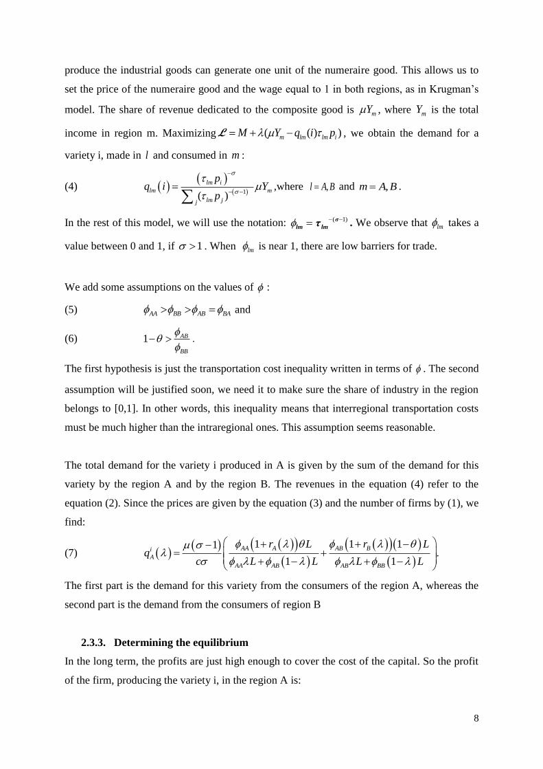
8

produce the industrial goods can generate one unit of the numeraire good. This allows us to

set the price of the numeraire good and the wage equal to 1 in both regions, as in Krugman’s

model. The share of revenue dedicated to the composite good is mY , where mY is the total

income in region m. Maximizing ( ( ) )m lm lm iM Y q i p L , we obtain the demand for a

variety i, made in l and consumed in m :

(4)

1( )   

lm i

lm m

lm jj

pq i Y

p

,where ,l A B and ,m A B .

In the rest of this model, we will use the notation: ( 1) σ

lm lm τ . We observe that lm takes a

value between 0 and 1, if 1  . When lm is near 1, there are low barriers for trade.

We add some assumptions on the values of   :

(5)    AA BB AB BA and

(6) 1 AB

BB

.

The first hypothesis is just the transportation cost inequality written in terms of . The second

assumption will be justified soon, we need it to make sure the share of industry in the region

belongs to [0,1]. In other words, this inequality means that interregional transportation costs

must be much higher than the intraregional ones. This assumption seems reasonable.

The total demand for the variety i produced in A is given by the sum of the demand for this

variety by the region A and by the region B. The revenues in the equation (4) refer to the

equation (2). Since the prices are given by the equation (3) and the number of firms by (1), we

find:

(7)

1 1 11.

1 1

AA A AB Bi

A

AA AB AB BB

r L r Lq

c L L L L

The first part is the demand for this variety from the consumers of the region A, whereas the

second part is the demand from the consumers of region B

2.3.3. Determining the equilibrium

In the long term, the profits are just high enough to cover the cost of the capital. So the profit

of the firm, producing the variety i, in the region A is:

9

(8) * *Π 0A AA AA AB AB AA AA AB ABi p i q i p i q i c q i q i fr

Let define the aggregate production as  A AA AA AB ABq i q i q i . Then we have:

(9) ( )

,( 1)

AA

cq ir

f

which can, using the demand functions defined by the equation (7), also be written as:

(10)

1 1 1.

1 1

AA A AB B

A

AA AB AB BB

r rr

f

Symmetrically, we find ( )Br :

(11)

1 1 1.

1 1

AB A BB B

B

AA AB AB BB

r rr

f

The spatial equilibrium is obtained when the returns in the two zones are the same. Therefore

we are looking for the value such that Ar and Br are equal:

1 1 .

1 1 1 1

AB BBAA AB

AA AB AB BB AA AB AB BB

After simplifications, we find (the share of industry in the central region):

(12)

,

AA AB AB BB

where Ψ 1 BB AB AB AB AA BB .

Proposition 1: If the interregional transportation cost is sufficiently large, compared to the

intraregional cost ( 1 BB AB ), there exists a unique interior equilibrium where the

industrial activity is shared between the two regions ( [0,1]  ). If the interregional cost is too

low ( 1 BB AB ), there is a corner solution and all the industrial activity is in the center

( 1 ).

The proof of this proposition is relegated to Appendix 1.

10

2.4.Comparative statics

One of the advantages of building our model on Helpman and Krugman (1985) is that we

have an analytical solution for the equilibrium. This allows comparative statics. Indeed, we

want to know the effects of improving the different types of infrastructure on the industrial

location patterns.

In this part, we modify the quality of a specific type of road and we evaluate its impact on the

distribution of industrial activity. We assume that the funds (and resources) for the realization

of this infrastructure are external. For instance, the funds could come from an international

development agency (World Bank) or be part of a federal effort to help peripheral regions

(Regional investment Fund in the EU). We show in Appendix 2 the following proposition.

Proposition 2: Both the improvement of the quality of interregional infrastructure and the

reduction of intraregional transportation costs in the center lead to a higher concentration of

industries in the center. However, lowering the peripheral intraregional transportation costs

increases the attractiveness of the periphery for firms.

Proposition 2 can be explained using the notion of market potential. As it was defined by

Harris (1954), and then extended by Head and Mayer (2004), the market potential is like a

weighted sum of the different potential sales on the national market and the surrounding

markets where a firm would like to export its product. The weights are inversely proportional

to the trade costs.

Since the center is bigger than the periphery, it has naturally a higher market potential, which

attracts firms. Reducing the interregional transportation costs will increase the market

potential of the center, because central firms will have a better access to the periphery.

Because of increasing returns, firms wish to move to the center. The reasoning is the same

with intraregional transportation cost in the center. However, a decrease of the intraregional

transportation cost in the periphery will increase the weight of the periphery in its market

potential. The market potential of the periphery will then increase, and will consequently

attract firms that will relocate from the center to the periphery.

11

3. Is this equilibrium efficient and can we improve it?

In this section, we first look for the efficiency benchmark: what geographical distribution of

industrial activity maximizes the sum of utilities in the two regions. The equilibrium we

described in the previous section is then compared to the benchmark. Next we look for

policies that could bring the equilibrium closer to the efficiency benchmark.

3.1. Computation of the indirect utility functions in the two regions

In order to maximize overall efficiency, we need an analytical expression for the utility in

both regions. Recall that 1U M A where 1 . Moreover, since A is the numeraire, then

the budget constraint reduces to: . 1P M A . Substituting into the utility function, we

obtain: 11 .( )U M PM

Maximizing the utility, with respect to M, and injecting the optimal value of M in the utility

function, we obtain the indirect utility function:

(13)

11

.VP

Moreover, we know that maximizing V is equivalent to maximizing any increasing

transformation of V . We will then rely on the following indirect utilities in this section:

(14) and .A A B BV P V P

In the new economic geography literature, the price index in the region A is given by:

(15)

1

1( .)1

A AA A AB B

cP n n

Using equation (1) for the number of firms, we obtain equation (16), which can be rewritten

as equation (17).

(16)

1

1(1 ),

1A AA AB

c L LP

f f

or

(17) ,1AA A ABKP

12

where

1

1

1

c LK

f

and

1.

1

We then have the indirect utility functions for an agent living in A ( AV ) and in B ( BV ) :

(18) ( (1 )) .A AA ABV K

Similarly, we obtain:

(19) ( (1 )) .B AB BBV K

3.2. Maximization of the total welfare in the economy

We start by looking for the maximum of the unweighted sum of utilities in the two regions.

There are two justifications for this. First one can allow for lump sum redistributive transfers

by a federal government. Second one can see the maximization of utilities as the basis for an

efficient bargaining between the two regions where the two regions share the gains of a better

equilibrium via transfers among themselves.

Since a share of the population is in the center (and 1 in the periphery), the welfare

function in the economy is then given by:

1 ,A BW V V

    1 1     1 .AA AB AB BBW K K

We look for the value o that maximizes the welfare function:

max max    1 1   1 .AA AB AB BBW W

The first order condition gives us the following value:

(20) ,o BB AB

BB AB AA AB

where

1

1

.1 BB AB

AA AB

13

We can note that 1 1 , and as a consequence: [0,1]o . The proof of these properties

is relegated to Appendix 3.

3.3. Comparison of the optimal and equilibrium values of the shares in industrial

activity

The question here is whether the concentration in the center is too high when the regulator

doesn’t intervene. To answer this question, we must compare the equilibrium value Eq and

the optimal value o . Recall that:

   ,Eq BB AB AB

BB AB AA AB

and that :

.o BB AB

AA AB BB AB AA AB BB AB

After some calculations (see Appendix 5), it can be shown that Eq o . The results are

summarized in:

Proposition 3: At equilibrium, the spatial concentration of industrial activity in the center is

too high compared to the first best optimum.

That the spatial equilibrium leads to a higher concentration than the first best optimum can

easily be understood. In fact, without any intervention, there is a kind of “snowball effect”

(the expression was first used by Myrdal in 1957). For a given level of infrastructures, the

center will attract firms. With these new firms, the market potential of the central region will

increase, attracting more firms and so on… If nothing is done by the regulator, there will be a

concentration of firms in the center that will be higher than the first-best optimum.

What would become of Prop. 3 when one gives a higher weight to peripheral citizens and

there would be no lump sum redistribution possible or no efficient bargaining between the

two regions? In Appendix 4 it is shown that a higher weight to peripheral citizens decreases

the value of the optimal share of industry in the center.. This is obvious since, giving a higher

14

importance to peripheral citizens, the concentration of firms in the center reduces the price

index in the periphery.

In order to improve total welfare, the concentration of firms in the center should be reduced.

This means that the government must intervene so as to favor the transfer of firms from the

center to the periphery.

3.4. Policies to reach the optimal location : the role of road pricing

In order to decentralize the social optimum o , we will use a set of incentives. In principle

one could use different instruments; the regulator could tax the firms in the center and/or

subsidize the firms in the periphery. Here, we focus on instruments that tax or subsidize the

use of transport infrastructures. This can be understood as a form of road pricing or as a

shadow cost used to compute the optimal size of different transport infrastructures. These

incentives will allow us to match o and Eq .

The intuition is clear from the outset, we will have to tax the use of the interregional road, tax

the use of the intraregional road in the center and/or subsidy the use of the intraregional road

in the periphery. The question is then to know the precise value of these taxes or subsidies.

3.4.1. Taxation of the use of the interregional road

We want to tax the interregional infrastructure. This is equivalent to reducing the value of

,AB which is the “freeness of trade”. To do this, we will look for the value t such that

AB AB ABt . We want to reach the value o , so we look for t , that solves :

).

1

(

AB AB ABBB AA BBo

AB ABAA BB

After some calculations, and solving the polynomial function in AB , we find :

(21) 2

21( 1) (1 ) 4 ( )( 1)

2( 1)

o o o o o o

AB AA BB BB AA AA ABo

15

Two remarks are in order:

Remark 1: From AB , we can find the value of .ABt

Remark 2: Reducing the value of AB to AB t is equivalent to increasing the iceberg cost

from AB to AB k . The value of k is then given by the following expression:

1

1 .AB AB ABk t

3.4.2. Taxation of the use of intraregional infrastructure in the center

We want to tax the use of intraregional infrastructure in the center. This is equivalent to

reducing the value of AA , which is the “freeness of trade”. To do this, we will look for the

value t such that AA AA AAt . We want to reach the value o , so we look for t , that

solves:

1.

AABB AB AB AB BBo

AA AB AB BB

After some calculations, and solving the polynomial function in AA , we find

(22) (1 )( )

.( )

BB AB ABAA AB o

AB BB BB

And the above remarks become:

Remark 1: From AA , we can deduct the value of .AAt

Remark 2: Reducing the value of AA to AA t is equivalent to increasing the iceberg cost

from AA to AA k . The value of k is then given by the following expression:

1

1 .AA AAk t

3.4.3. Subsiding of the use of the intraregional road in the periphery

16

We want to subsidize the use of the intraregional infrastructure in the periphery. This is

equivalent to increasing the value of BB , which is the “freeness of trade”. To do this, we will

look for the value of the subsidy s such that .BBB BB Bs

We want to reach the value o , so we look for 'BB , that solves:

1.

( )

BB BBAB AB AB AAo

BBAA AB AB

After some calculations, we obtain:

(23) 2 (1 )

.(1 ) ( )

o o

AA AB AB

o o

AB AA

BB

Remark 1 : From BB , we can deduct the value of BBs .

Remark 2 : Increasing the value of BB to BB s is equivalent to reducing the iceberg cost

from BB to BB k . The value of k is then given by the following expression:

1

1 .BB BB BBk s

We have developed a set of incentives such that the equilibrium will be the optimal one. To

do this, we focused on road pricing. One can reach the optimum in three different ways:

taxing the use of the interregional infrastructure; taxing the use of the intraregional

infrastructure in the center or subsidizing the use of the intraregional infrastructure in the

periphery. Note that subsidizing the intraregional infrastructure in the periphery does not

mean building a road. Indeed, the creation of the infrastructure is costly, while a subsidy is in

principle a mere transfer of resources that corrects incentives and is not consuming real

resources (except for the transaction costs). We illustrate our model below with a numerical

example.

3.4.4. A numerical example: Mozambique and Malawi

In order to illustrate the mechanisms of the model, we take a numerical example. Since

comprehensive data on interregional and intraregional transportation costs for road transport

17

are difficult to gather, we use from UNCTAD (2004). In their report, they calculate very

accurate values for transportation costs in Africa. We take the example of two countries,

instead of two regions. This choice is mainly due to the availability of data, but especially

because it does not change anything concerning the assumptions and results. The two selected

countries are Mozambique (the center) and Malawi (the periphery).

First, we must calibrate our model. To do so, we match real data with the various parameters

we use in the model. Table 1a displays values for the central country, whereas table 1b does it

for the periphery.

Table 1a. Numerical values for the parameters of Mozambique

Region A – The core Mozambique

Population 19M

Share of the population

0.6

Infrastructure quality

index

23.1

AA 0.9

Table 1b. Numerical value for the parameters of Malawi

Region B – The Periphery Malawi

Population 13M

Share of the population

1

0.4

Infrastructure quality index 20.4

BB 0.79

18

Once these parameters have been calibrated, we must set the values of other parameters, that

are not always known (for instance ). Others, like the interregional transportation cost, can

be found in UNCTAD (2004) .

Table 2. Other parameters to run the simulation

Other parameters

w wage 1

(elasticity of substitution) 6

Share of transport cost in the price

of goods sold in the other region

22%

Iceberg cost AB 1.28

AB 0.29

0.6

Note that several values have been tested for the elasticity of substitution, and they do not

change dramatically the results. We can now compute the spatial equilibrium and the spatial

optimum. It is interesting to note that the simulated spatial equilibrium ( 0.75 ) is very

close to the real value ( 0.74 ).

Table 3. Spatial equilibrium and spatial optimum

Spatial equilibrium and optimum

Spatial equilibrium Eq 0.75

Intermediate parameter 1.59

Optimal concentration o 0.69

As predicted by Proposition 3, there is a significant difference between the spatial equilibrium

and the optimal concentration. The next step is to calculate the values of the different taxes or

subsidies to reach the optimal concentration.

19

Table 4. Optimal taxes and subsidies on use of infrastructure to reach the optimum and

their impact on the transportation costs

Road pricing to reach the equilibrium

Optimal AA

Optimal tax AAt

0.74

0.16

Optimal AB

Optimal tax ABt

0.20

0.09

Optimal BB

Optimal subsidy BBs

0.91

0.12

From these new values of transportation costs, we can deduct the impact on the product

prices:

Table 5. Impact of taxes on transportation costs

Share of the transport cost in the price of a shipped

product

Before tax After tax

Interregional 22% 27%

Intraregional in the center 2% 6%

Intraregional in the periphery 4% 2%

This numerical example illustrates the different values predicted by our model. The values of

the various taxes or subsidies are not unrealistic. These numerical simulations confirm that

the predictions of our model are in line with the theoretical results. At equilibrium, the

concentration of activities in the center is too high and the use of interregional road taxes can

restore the optimum.

20

CONCLUSION

If a whole literature has studied the impact of transportation costs on the geographical

distribution of activities, this paper is among the first to analyze the specific roles of

interregional and intraregional transport costs .

Several conclusions can be drawn from this paper. First, the improvements of the different

categories (interregional/intraregional) of infrastructures have different effects on industrial

location. We confirm Martin and Rogers (1995analysis: if the decision maker whishes to use

the transport policy to reduce regional inequalities, then s/he must improve the quality of the

peripheral intraregional infrastructure. The second conclusion follows from the normative

analysis. Indeed, we show that the spatial equilibrium is far from being Pareto optimal.

Without any intervention, the spatial equilibrium will lead to a concentration of firms in the

center that is too high. The third result is that it is possible to use tax and subsidy instruments

such as road pricing to reach the optimal share of firms in the center.

Yet, this model could be improved in several ways. First, it was designed in such a way that

interregional and intraregional transportation costs were independent. In reality, mattters are

more complex and intraregional infrastructures may affect directly the interregional

transportation costs. These network effects must be taken into account if we want a more

realistic view of the effects of infrastructures on industrial location. Second, the introduction

of congestion costs within regions would probably give interesting results. As it was

explained by Lafourcade and Thisse (2011), congestion costs moderate the spatial

polarization of activities. In our model, they would affect strongly the optimal taxes and

subsidies. With these improvements, future research allows to understand more properly the

dynamics of spatial activities.

21

REFERENCES

W. Alonso (1964), Location and Land Use, ed. Harvard University Press

P. Bairoch (1989), « European Trade Policy, 1815-1914 », in Cambridge Economic

History of Europe (by Mathias and Pollard), ed. Cambridge University Press

P. Bairoch (1997), Victoires et déboires. Histoire économique et sociale du monde du

XVIe siècle à nos jours, ed. Gallimard

K. Berhens and J.-F. Thisse (2007), « Regional economics: a new economic geography

perspective », Regional Science and Urban Economics, vol. 37, n°4, pp. 457-465

J. Cavailhes, C. Gaigne, T. Tabuchi and J.-F. Thisse (2006), « Trade and the structure of

cities », Journal of Urban Economics, vol.62, n°3, pp. 383-404

D. Cohen (2004), La mondialisation et ses ennemis, ed. Grasset

C. Harris (1954), « The market as a factor in the localization of industry in the United

States », Annals of the Association of American Geographers, vol. 44, pp. 315-348

K. Head and T. Mayer (2004), « Market potential and the location of Japanese firms in the

European Union », The Review of Economics and Statistics, vol. 86, n°4, pp. 959-972

E. Helpman and P. Krugman (1985), Market structure and Foreign Trade, ed. MIT Press

P. Krugman (1980), « Scale economies, product differentiation and the pattern of trade »,

American Economic Review, vol. 70, n°5, pp. 950-959

P. Krugman (1991), «Increasing returns and economic geography », Journal of Political

Economy, vol. 99, n°3, pp. 493-499

M. Lafourcade and J-F. Thisse (2011), « New economic geography : The role of transport

costs », in A. de Palma, R. Lindsey, E. Quinet and R. Vickerman (eds) (2011), Handbook

in Transport Economics, ed. Edward Elgar

A. Marshall (1890), Principles of Economics, ed. MacMillan

P. Martin and C. Rogers (1995), « Industrial location and public infrastructure », Journal

of International Economics, vol. 39, n°3, pp. 335-351

G. Myrdal (1957), Economic Theory and Underdeveloped Regions, ed. Gerald Duckworth

D. Puga (1999), « The Rise and Fall of Regional Inequalities », European Economic

Review, vol. 43, n°2, pp. 303-334

T. Tabuchi (1998), « Urban Agglomeration and Dispersion: A synthesis of Alonso and

Krugman », Journal of Urban Economics, vol. 44, n°3, pp. 333-351

Unctad (2004), World Trade Report 2004

R. Vickerman (1991), Infrastructure and regional development, ed. Pion

22

R. Vickerman, K. Spiekermann, and M. Wegener (1999), « Accessibility and Economic

development in Europe », Regional Studies, vol.33, n°1, pp. 1-15

23

Appendix 1. Proof of Proposition 1

We want to prove that 1AB BB , then [0,1]

Proof of 0

We know that: 0AA AB AB BB . If 0 , then we must have Ψ 0 . Let’s prove it

by contradiction. If Ψ 0 , then we have

Ψ 1 0BB AB AB AB AA BB

.1 BB AB AB AA AB BB

Since 1   and BB AB AA AB and since AB BB , the previous line ca not be true.

This means that Ψ 0 , and then 0 .

Proof of 1

We know that 0AA AB AB BB . If 1 , then we must have :

1 BB AB AB AB AA BB AA AB AB BB

1 0.BB AB AB AB AA BB AB BB

Since  1 0BB AB and 0AB AA , we must have 0BB AB BB which is

true if 1 .  .AB BB

Proof that if 1AB BB , then 1

We know that: 0AA AB AB BB . If 1 , then we must have:

1 BB AB AB AB AA BB AA AB AB BB

.BB AB AA AB AA AB BB

Since   1AB BB , then   1AB BB , so we have

( ).BB AB AA AB BB AA AB

24

Moreover, we can note that:  AA AB AA AB . So we can conclude that we have:

BB AB AA AB AA AB BB , which means that if 1AB BB , then 1 .

Appendix 2. Proof of Proposition 2

Impact of AB : Improving the quality of the interregional infrastructure is like an increase in

AB .

2

1 2  Ψ[ 2 ]BB AB BB AA AB AB BB AA BB AB

AB AA AB AB BB

We have: 0 

AB

λif the condition 2AA

AB

is respected (which always holds with our

assumptions). Using this hypothesis, we observe that the improvement of the infrastructure

between regions will strengthen the concentration in the center.

Impact of AA : We measure the effects of an improvement of infrastructures in the center.

We expect that it will lead to a higher concentration in the center.

2

[ ]Ψ 

BB AA AB AB BB AB BB

AA AA AB AB BB

We obtain: 0

AA

λ. As predicted, we conclude that the higher quality of infrastructure in

the center will increase the concentration.

Impact of BB  : Since the other actions on infrastructures have led to a higher concentration,

we expect that the reduction of transport costs in the periphery will lead to a reduction of the

concentration in the center.

25

2

1 [ ]ΨAB AB AA AA AB AB BB AA AB

BB AA AB AB BB

We find that 0

BB

λ if we have  AB AA (which holds with our hypotheses) .The better

quality of infrastructure in the periphery will lead to a relocation of firms from the center to

the periphery.

Appendix 3. Remarks concerning the value of ζ

First, we want to show that 0 1

We can rewrite as:

1 1

1 1

.1

ΩBB AB BB

AA AB AA

Since 0 Ω 1 and BB AA , we can conclude than 0 1.

Second, we want to show that 1

Let’s prove it by contradiction. Then we make the hypothesis that 1 .

So we must have:

1 111 1

11

1   1  (1 )  BB AB BB AB

AA AB AA AB

11 11

1 (1 ) .AA AB

BB AB

Since 1 1

1 1

and since 0 1 1 then we have :

1 11

1 1(1 ) (1 ) .

We can then rewrite the inequality:

11 1

1(1 )   1    1 .1

AA AB AA AB AA AB

BB AB BB AB BB AB

26

And this is false. So by contradiction, we can say that 1 θ

Third, with 1 1 , then we have [0,1]o

We know that 1 . Since we have shown that 1 BB AB , we now have:

.BB AB

This allows us to say that:

[0,1].

 o BB AB

BB AB AA AB

ζλ    

ζ ζ

Appendix 4. Impact of the weights on the optimal value of industry share

We want to assess the impact of the weights in the total utility function on the optimal value

of the industry share. To do this, we normalize the weight for region A to 1 and give a weight

to region B. This way, the indirect utility function to be maximized is then:

1A BW V V

max max    1 1   1AA AB AB BBWW

The first order condition gives us the following value:

,

 o BB AB

BB AB AA AB

λ  

where

1

11 BB AB

AA AB

.

It is easy to show that 0

. Moreover, one can prove that

 

0o

. Knowing the signs of

these two derivatives, we can then conclude that an increase in will lead to a reduction of

 o .

27

Appendix 5. Proof of Proposition 3

The spatial equilibrium is given by the value Eq :

1 

( )

BB AB AB AB AA BBEq

AA AB AB BB

Eq BB AB AB

BB AB AA AB

.

We want to compare Eq with the optimal share of firms o that can be rewritten as:

( ) ( )

o BB AB

AA AB BB AB AA AB BB AB

First, we can compare the second parts of the two equations. Since   0BB AB and

0AB , then we can observe that:

( )

AB AB AB

AA AB AA AB BB AB

.

Second, we want to compare the first parts of the equations. Let’s prove by contradiction that

( )

BB BB

BB AB AA AB BB AB

To do so, we make the hypothesis that:

 ( )

BB BB

BB AB AA AB BB AB

This would mean that :

  AA AB BB AB BB AB

  1 0AA AB BB AB

1 ( )

AA AB

BB AB

1 .

28

This is a contradiction since we know that 0 1 . So this means that we have:

.( )

BB BB

BB AB AA AB BB AB

These two inequalities lead us to the conclusion that: Eq oλ λ .