the impact of capital structure on profitability. evidence
TRANSCRIPT

The impact of capital structure on profitability. Evidence from
the FTSE 100 and FTSE 250.
Serafeimidis Antonios
SCHOOL OF ECONOMICS, BUSINESS ADMINISTRATION & LEGAL STUDIES
A thesis submitted for the degree of
Master of Science (MSc) in Banking and Finance
December 2019 Thessaloniki – Greece

I hereby declare that the work submitted is mine and that where I have made use of another’s work, I have attributed the source(s) according to the Regulations set in the Student’s Handbook.
December 2019
Thessaloniki - Greece
Student Name: Antonios Serafeimidis
SID: 1103180019
Supervisor: Prof. Athanasios Fassas

iii
Abstract
This dissertation was written as part of the MSc in Banking and Finance at the
International Hellenic University.
The present study addresses the effect of capital structure on profitability of listed
non-financial firms in the London Stock Exchange and more especially in FTSE 100
and FTSE 250 Indexes. The objectives of the study are to identify the nature of the
relationship between capital structure and firm performance, as well as explore the
impact of capital structure on firm performance.
The issue is important since the capital structure is a decision that firms take
and influence all stakeholders. Models structured as having dependent variables
ROA, ROE, and Gross Profit Margin, whereas Debt (Long term debt, Short term debt
and Total debt) was the independent variable. Research models were developed for
each group of the data as well as for each independent variable. The Simple linear
regression analysis conducted using OLS, fixed effects, and random effects methods.
According to the research results, capital structure affects profitability, to a
greater or lower extent. There is not a specific rule for firms to follow since the
capital structure is also an internal decision and can be affected by several factors.
Nevertheless, the present study adds in the existing literature by confirming previous
research results as well as by revealing new relationships between the variables
selected for the research.
Keywords: capital structure, leverage, profitability, index analysis
Antonios Serafeimidis
15/12/2019

iv
Preface
This thesis is consecrate to the memory of my father Ilias.
First of all, I would like to thank my professor Athanasio Fassa for his valuable
support and contribution, but also his orientation and correspondence to all my
questions for this project. As well as my family for the patience they showed during
the difficult and demanding period of the preparation of the present study. Also, I
would like to thanks my friend Kostas for his contribution. I would also like to
acknowledge the hospitality of all the personnel of the International Hellenic
University. Last but not least I would like to thank my friends that I met during my
MSc in IHU and specifically, Stelios Grigoriadis, Aris Vaitsidis and Nikolaos
Moutzoglou.
Thank you all for your support.

v
vi
Table of Contents
Abstract ..................................................................................................................................... iii
Preface ...................................................................................................................................... iv
2.Introduction ........................................................................................................................... 1
2.1 Purpose of this Study ....................................................................................................... 1
2.2 The Structure of this Study .............................................................................................. 1
3.Literature Review .................................................................................................................. 3
3.1 The determinants of capital structure ............................................................................. 3
3.1.1 The size of a firm ...................................................................................................... 3
3.1.2 Asset tangibility ........................................................................................................ 3
3.1.3 Growth ...................................................................................................................... 4
3.1.4 Profitability ............................................................................................................... 4
3.1.5 Debt tax shields ........................................................................................................ 4
3.1.6 Non-debt-tax shield .................................................................................................. 5
3.1.7 Age ............................................................................................................................ 5
3.1.8 Risk............................................................................................................................ 5
3.2 The impact of Capital Structure on Profitability .............................................................. 6
4.Research Methodology ........................................................................................................ 23
4.1 Data ............................................................................................................................... 23
4.2 Modeling ........................................................................................................................ 24
4.3 Population ..................................................................................................................... 25
4.4 Research Hypotheses ..................................................................................................... 25
5.Empirical Results & Analysis................................................................................................ 27
5.1 FTSE 100 Period: 2002 – 2010 ....................................................................................... 27
5.2 FTSE 100 Period: 2011 – 2018 ....................................................................................... 47
5.3 FTSE 250 Period: 2002 - 2010 ........................................................................................ 65
6.4 FTSE 250 Period: 2011 – 2018 ....................................................................................... 82
6.Conclusions ........................................................................................................................ 100
6.1 Key Results ................................................................................................................... 100
6.2 Further Research ......................................................................................................... 103
Bibliography .......................................................................................................................... 104
Appendix ................................................................................................................................... 1
vii
List of Figures
Figure 1: Hypothesized Relations among the selected variables, Tailab (2015, p.56) ........... 15
Figure 2: conceptual model, source: Stekla & Grycova (2015, p. 35) ..................................... 17
Figure 3: Number of Companies for each Sector .................................................................... 27
Figure 4: Number of Companies for each Sector .................................................................... 65
List of Tables
Table 1: Descriptive statistics for FTSE100 data for the years 2002-2010 .............................. 28
Table 2: Correlation matrix for FTSE100 data for the years 2002-2010.................................. 29
Table 3: Regression Analysis Results, ROA/Short-term Debt. Method Random Effects, period
2002-2010, FTSE100 ................................................................................................................ 31
Table 4: Regression Analysis Results, ROA/Long-term Debt. Method Random Effects, period
2002-2010, FTSE100 ................................................................................................................ 33
Table 5: Regression Analysis Results, ROA/Total Debt. Method Random Effects, period 2002-
2010, FTSE100 ......................................................................................................................... 35
Table 6: Regression Analysis Results, ROE/Short-term Debt. Method Random Effects, period
2002-2010, FTSE100 ................................................................................................................ 37
Table 7: Regression Analysis Results, ROE/Long-term Debt. Method Random Effects, period
2002-2010, FTSE100 ................................................................................................................ 39
Table 8: Regression Analysis Results, ROE/Total Debt. Method Random Effects, period 2002-
2010, FTSE100 ......................................................................................................................... 41
Table 9: Regression Analysis Results, Gross Profit Margin/Short-term Debt. Method Random
Effects, period 2002-2010, FTSE100 ........................................................................................ 43
Table 10: Regression Analysis Results, Gross Margin/Long-term Debt. Method Random
Effects, period 2002-2010, FTSE100 ........................................................................................ 45
Table 11: Regression Analysis Results, Gross Margin/Total Debt. Method RE, period 2002-
2010, FTSE100 ......................................................................................................................... 46
Table12: Descriptive statistics for FTSE100 data for the years 2011-2018 ............................. 47
Table 13: Correlation matrix for FTSE100 data for the years 2011-2018................................ 48
Table15: Regression Analysis Results, ROA/Long-term Debt. Method Random Effects, period
2011-2018, FTSE100 ................................................................................................................ 51
Table 17: Regression Analysis Results, ROE/Short-term Debt. Method Random Effects, period
2011-2018, FTSE100 ................................................................................................................ 55
Table 18: Regression Analysis Results, ROE/Long-term Debt. Method Random Effects, period
2011-2018, FTSE100 ................................................................................................................ 57

viii
Table 19: Regression Analysis Results, ROE/Total Debt. Method Random Effects, period
2011-2018, FTSE100 ................................................................................................................ 59
Table 20: Regression Analysis Results, Gross Profit Margin/Short-term Debt. Method
Random Effects, period 2011-2018, FTSE100 ......................................................................... 61
Table 21: Regression Analysis Results, Gross Profit Margin/Long-term Debt. Method Random
Effects, period 2011-2018, FTSE100 ........................................................................................ 62
Table 22: Regression Analysis Results, Gross Profit Margin/Total Debt. Method Random
Effects, period 2011-2018, FTSE100 ........................................................................................ 64
Table 23: Descriptive statistics for FTSE250 data for the years 2002-2010 ............................ 65
Table 24: Correlation matrix for FTSE250 data for the years 2002-2010................................ 66
Table 25: Regression Analysis Results, ROA/Short-term Debt. Method Random Effects,
period 2002-2010, FTSE250 ..................................................................................................... 68
Table 26: Regression Analysis Results, ROA/Long-term Debt. Method Random Effects, period
2002-2010, FTSE250 ................................................................................................................ 70
Table 27: Regression Analysis Results, ROA/Total Debt. Method Random Effects, period
2002-2010, FTSE250 ................................................................................................................ 72
Table 28: Regression Analysis Results, ROE/Short-term Debt. Method Random Effects, period
2002-2010, FTSE250 ................................................................................................................ 74
Table 29: Regression Analysis Results, ROE/Long-term Debt. Method Random Effects, period
2002-2010, FTSE250 ................................................................................................................ 75
Table 30: Regression Analysis Results, ROE/Total Debt. Method Random Effects, period
2002-2010, FTSE250 ................................................................................................................ 77
Table 31: Regression Analysis Results, Gross Profit Margin/Short-term Debt. Method
Random Effects, period 2002-2010, FTSE250 ......................................................................... 78
Table 32: Regression Analysis Results, Gross Margin/Long-term Debt. Method Fixed Effects,
period 2002-2010, FTSE250 ..................................................................................................... 79
Table 33: Regression Analysis Results, Gross Profit Margin/Total Debt, Method FE, period
2002-2010, FTSE250 ................................................................................................................ 81
Table 34: Descriptive statistics for FTSE250 data for the years 2011-2018 ............................ 82
Table 35: Correlation matrix for FTSE250 data for the years 2011-2018................................ 83
Table 36: Regression Analysis Results, ROA/Short-term Debt. Method Random Effects,
period 2011-2018, FTSE250 ..................................................................................................... 85
Table 37: Regression Analysis Results, ROA/Long-term Debt, Method FE, period 2011-2018,
FTSE250 ................................................................................................................................... 86
Table 38: Regression Analysis Results, ROA/Total Debt. Method Fixed Effects, period 2011-
2018, FTSE250 ......................................................................................................................... 88

ix
Table 39: Regression Analysis Results, ROE/Short-term Debt. Method Random Effects, period
2011-2018, FTSE100 ................................................................................................................ 90
Table 40: Regression Analysis Results, ROE/Long-term Debt. Method Random Effects, period
2011-2018, FTSE250 ................................................................................................................ 92
Table 41: Regression Analysis Results, ROE/Total Debt. Method Random Effects, period
2011-2018, FTSE250 ................................................................................................................ 94
Table 42: Regression Analysis Results, Gross Profit Margin/Short-term Debt. Method Fixed
Effects, period 2011-2018, FTSE250 ........................................................................................ 95
Table 43: Regression Analysis Results, Gross Margin/Long-term Debt. Method Fixed Effects,
period 2011-2018, FTSE250 ..................................................................................................... 97
Table 44: Regression Analysis Results, Gross Profit Margin/Total Debt, Method FE, period
2011-2018, FTSE250 ................................................................................................................ 98

1
2.Introduction
2.1 Purpose of this Study
The financing decision is very important for companies since financing represents the
way that firms use to fund their operations. The basic financing decision is whether a
company will seek funding by issuing equity either by using their earnings or by
borrowing from financial institutions. There are a lot of different determinants that
firms use to choose the ideal capital structure, i.e. the proportion of debt in their
assets. Profitability is one of these determinants and examined in the present study.
Specifically, this study addresses the effect of capital structure on profitability of
listed non-financial firms in the London Stock Exchange and more especially in FTSE
100 and FTSE 250 Indexes. The objectives of the study are to:
i. Identify the nature of the relationship between capital structure and firm
performance.
ii. Explore the impact of capital structure on firm performance.
2.2 The Structure of this Study
In order to fulfill the project’s aim, the study structured as follows. First, the
literature review on the subject realized. The literature review concentrates on the
determinants of capital structure as well as previous research on the impact of
Capital Structure on profitability. The capital structure represents a very important
but also complex decision for companies because it is highly related to several other
aspects of the organizational performance, as well as external environmental factors.
As mention above, widely presented during the literature review section.
Then research methodology and results follow — the present cross-sectional
study based on secondary research data. The data from the annual financial report
and Thomson- EIKON database collection were administrated contemporaneously
for the entire selected population. The descriptive analysis used to systematize and
present the data. Panel data analysis was used, beginning with the calculation of
mean, median and standard deviation to transmit the orientation of the distribution

2
of overall data. Correlation tests were conducted to observe the correlation
coefficient of variables at significant levels (5% and 10%). Then, the simple linear
regression analysis conducted using OLS, fixed effects and random effects methods.
Furthermore, research models presented, and research analysis follows. Last,
concluding remarks follow.

3
3.Literature Review
3.1 The determinants of capital structure
Capital structure is an issue that has long occupied economists all over the world. It
is highly related to market value, and firms wish to find the best combination to
achieve the ultimate profitability and market value. Researchers have used data of
different kinds of firms in terms of volume, sector, and country in which they
operate. The theory on Capital structure based on Modigliani & Miller's (1958) work
argued that the need for making decisions on a capital structure derived by the fact
that the markets are not frictionless. Instead, there are some elements in the
markets, such as the risk of bankruptcy or the need to pay taxes, which makes the
capital structure of firms important for their value increase. Moreover, researchers
who have dealt with capital structure note that there are several factors, such as
taxation, financial distress costs or regulatory decisions, which influence a firm’s
change in value, thus an optimal degree of leverage need to be found by each
company. Research has revealed that the determinants of capital structure are the
following:
3.1.1 The size of a firm
As far as the size of the firms concerned, it would be expected – as the pecking order
theory suggests - that large firms generate more profits than small ones. Thus, they
have the resources to fund their operations.
On the other hand, there is the theory according to which large firms are
prone to leverage since the debt interest rate is deductible. Also, it is easier for large
firms to access the debt market because they are more reliable, enjoy lower
information asymmetry and are more diversified. It is obvious that, generally,
researchers tend to support the idea that large firms are probable to leveraged than
smaller ones (Sibindi, 2016).
3.1.2 Asset tangibility
Tangible assets are the assets that lenders value more in a transaction than
intangible ones. They represent assets that can be used as collaterals when firms
4
need to borrow, something that reduces the risk for lenders. Thus, according to the
trade-off theory, as firms grow and their tangible assets grow, they are more likely to
borrow more (Antoniou et al., 2008). As a result, there is a positive relationship
between debt and asset tangibility. On the other hand, some researchers support
the argument that high tangibility is related to low information asymmetry,
something that reduces equity issuance cost and leads to a negative relationship
between asset tangibility and leverage (Frank & Goyal, 2009).
3.1.3 Growth
According to the trade-off theory, growth negatively related to debt, since growth
offers greater value to shareholders, the cost of financial distress increases, and
firms prefer to reduce debt. Besides, growing firms that expect to grow further, issue
equity instead of debt (Barkley & Smith, 2005). On the other hand, some researchers
argue that growing firms are more probable to have financing needs, and –
according to the pecking order theory – they issue debt before equity (Sibindi, 2016).
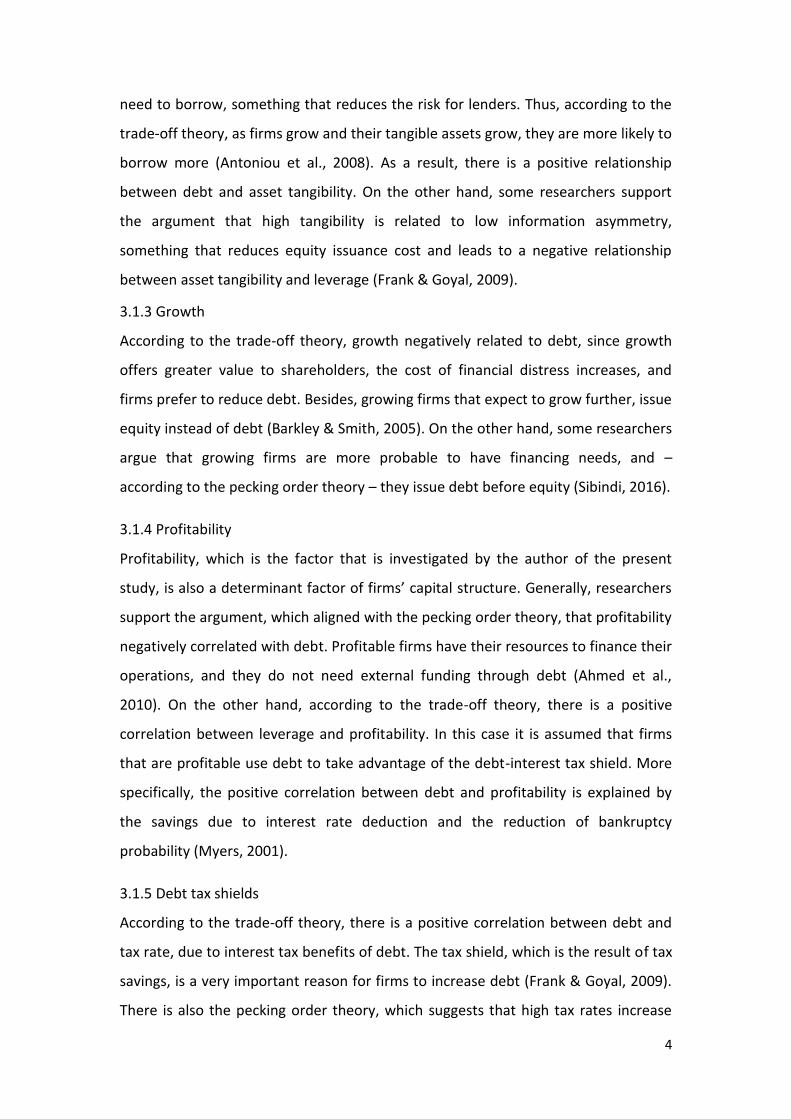
3.1.4 Profitability
Profitability, which is the factor that is investigated by the author of the present
study, is also a determinant factor of firms’ capital structure. Generally, researchers
support the argument, which aligned with the pecking order theory, that profitability
negatively correlated with debt. Profitable firms have their resources to finance their
operations, and they do not need external funding through debt (Ahmed et al.,
2010). On the other hand, according to the trade-off theory, there is a positive
correlation between leverage and profitability. In this case it is assumed that firms
that are profitable use debt to take advantage of the debt-interest tax shield. More
specifically, the positive correlation between debt and profitability is explained by
the savings due to interest rate deduction and the reduction of bankruptcy
probability (Myers, 2001).
3.1.5 Debt tax shields
According to the trade-off theory, there is a positive correlation between debt and
tax rate, due to interest tax benefits of debt. The tax shield, which is the result of tax
savings, is a very important reason for firms to increase debt (Frank & Goyal, 2009).
There is also the pecking order theory, which suggests that high tax rates increase

5
the cost of capital for firms, something that leads to a negative relationship between
tax rate and debt of a firm (Rasiah & Kim, 2011).
3.1.6 Non-debt-tax shield
Generally, researchers agree that there is negative correlation between leverage and
non-debt tax shield. According to them, tax deductions for depreciation, or other
intangible assets, substitute tax benefits from lending. Thus, firms that enjoy non-
debt tax shields have lower leverage levels (Frank & Goyal, 2009). Some researchers
support the inverse, where there is positive correlation between debt and non-debt-
tax shields. Nevertheless, this is attached to firms’ anomalous behavior (Sibindi,
2016).
3.1.7 Age
Age is a determinant factor of capital structure because it is related to characteristics
that are related to decisions on capital structure. The most important factor is
reputation, where old firms enjoy a better reputation, thus lower lending costs,
something that creates a positive relationship between age and leverage (Harris &
Raviv, 1991). On the other hand, old firms are expected to be more profitable. Thus,
it is easier for them to finance their needs by using their internal resources (Ahmed
et al., 2010).
3.1.8 Risk
Risk is a term that is related to firms’ performance. It is an indicator of the volatility
of the earning of a company. According to the trade-off theory, there is negative
correlation between risk and debt. It argued that when the risk is high, the
probability of the firm not being able to fulfill its commitments concerning debt
increased. So is the probability of bankruptcy. Thus, companies that demonstrate
volatile earnings should avoid leverage (Antoniou et al., 2008). On the other hand,
the pecking order theory supports the positiverelationship between debt and risk,
because in this way the adverse selection problem is avoided (Frank & Goyal, 2009).
Below, a literature review on the impact of one of these determinants,
profitability, on the Capital Structure presented.
6
3.2 The impact of Capital Structure on Profitability
Below, an extended literature review on the subject is presented to set the
theoretical framework for the empirical part of the present study, the impact of
Capital Structure on the Profitability of Companies listed in the London Stock
Exchange, and belonging to the FTSE 100 and the FTSE 250 index. The literature
review that follows is presented by the date, starting from the earlier research on
the subject.
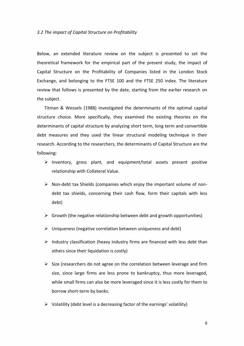
Titman & Wessels (1988) investigated the determinants of the optimal capital
structure choice. More specifically, they examined the existing theories on the
determinants of capital structure by analyzing short term, long term and convertible
debt measures and they used the linear structural modeling technique in their
research. According to the researchers, the determinants of Capital Structure are the
following:
Inventory, gross plant, and equipment/total assets present positive
relationship with Collateral Value.
Non-debt tax Shields (companies which enjoy the important volume of non-
debt tax shields, concerning their cash flow, form their capitals with less
debt)
Growth (the negative relationship between debt and growth opportunities)
Uniqueness (negative correlation between uniqueness and debt)
Industry classification (heavy industry firms are financed with less debt than
others since their liquidation is costly)
Size (researchers do not agree on the correlation between leverage and firm
size, since large firms are less prone to bankruptcy, thus more leveraged,
while small firms can also be more leveraged since it is less costly for them to
borrow short-term by banks.
Volatility (debt level is a decreasing factor of the earnings’ volatility)
7
Profitability (profitability is negatively correlated to debt since firms prefer to
use their capitals as a result of asymmetric information and transaction costs)
The variables used by Titman & Wessels (1988), as Capital structure measures
are long term debt, short term debt, and convertible debt, dividend by market and
dividend by the book value of equity. They used data from 469 firms in the USA
during the period 1974-1982. According to their linear structural modeling technique
results, debt negatively related to the uniqueness of a firm. Also, transaction costs
affect debt structure, while short term debt is negatively related to firm size.
Voulgaris et al. (2002), tried to reveal the factors that influence capital structure
of Large Size Enterprises (LSEs) in Greece, to present the implications involved after
the financial integration of Greece and the EU, under the use of the single monetary
unit, the euro. According to the researchers, there are three major theories
concerning the capital structure of companies and are based on the so call M-M
(from Modigliani & Miller) model, where only the ability of a company to generate
profit affects its market value, whereas the company’s financial structure does not
affect market value. The first theory based on the tax advantages that a company
has due to its debt. According to this theory, companies that generate high profits
should use more debt than equity, since interest rates have tax benefits. Of course,
this choice leads to a tradeoff between tax benefits and increased bankruptcy
possibility, something that may increase the cost of capital. The second theory is
known as the “agency cost” theory where firms finance their needs according to the
following order: first, they use funds that are created internally by the firm’s
operation, then they use debt and, last, they issue new equity. Thus, profitability and
debt are negatively related. The third theory is asymmetric information. According to
this theory, companies with large free cash flow and low growth opportunities tend
to have higher levels of debt. Also, according to the asymmetric information theory,
capital structure depends on the firms’ size. Consider the previous theory; there is a
positive correlation between debt and asset structure.
Voulgaris et al. (2002) used data of the Balance Sheets and the Income
Statements of 75 Greek manufacturing LSEs. They calculated twenty-two financial
ratios, which belong to the following categories:

8
Solvency
Managerial Performance
Profitability
Growth
The dependent variables of their model were Total Debt/Total Assets, Long-term
Debt/Total Debt, and Short-term Debt/Total Assets. According to the results of their
analysis, there is negative correlation between Total Debt and profitability. In other
words, LSEs prefer to use their profits to finance their activities; the higher the
profits, the lower the debt.
Furthermore, profitability was found correlated with long term debt, rather than
short-term borrowing, while total debt correlated to Total Assets turnover.
Companies with high growing ratios and financing needs seem to prefer debt to new
equity issuing. Besides, long term debt is positively affected by gross profit margins
and negatively correlated with assets productivity and growth, as well as sales.
Voulgaris et al. (2002) did not find significant correlation between capital structure
and ratios such as return on equity and asset profitability.
Pasiouras & Kosmidou (2007) examined the factors that influence profitability in
the case of foreign and domestic banks in the EU 15, for the years 1995 – 2001.
Deregulation, according to the authors, was a factor that enhanced competition
among banks in the EU15, since the official authorities permitted more freedom
concerning the establishment, operation, and control of banks. Competition
increased and banks needed to issue new, attractive financial products for their
customers. Also, mergers and acquisitions used as a strategy that helped banks
become larger and more competitive. All these changes were vital, and the authors
wished to examine the factors that affect profitability in this new environment.
Pasiouras & Kosmidou (2007) used their model’s dependent variable Return on
Average Assets (ROAA), which is an indicator of the profits earned per euro of assets.
The independent variables of their model based on both internal and external
factors. Internal factors were measured using the following:

9
Capital adequacy ratio
Cost/ Income Ratio
Liquidity Ratio
Size (accounting value of assets)
Macroeconomic factors’ measures were inflation rate, gross GDP, Total deposits
/ GDP, Stock Market Capitalization / Total Assets, Stock Market Capitalization / GDP,
Concentration (Assets of the five major banks / Total assets of banks).
The researchers used a sample of 584 commercial banks, form the EU15
countries, for the years 1995 – 2001. They further divided their sample into two sub-
categories, domestic banks (332 banks) and foreign banks (218 banks), while 34
banks not classified at this second stage. According to research results, all
independent variables, except for concentration in the case of domestic banks, were
found significant for banks’ profitability. Capital adequacy and Cost / Income Ration
seem to be the most important determinant of profitability. The cost of income has a
significant, negative correlation with profitability, especially in the case of foreign
banks. Liquidity is positively correlated with profitability, in the case of domestic
banks, whereas it negatively correlated with profitability in the case of foreign banks.
Size in negatively correlated to profitability, for domestic as well as for foreign banks.
Furthermore, all macroeconomic factors affect profitability, but in different ways
for domestic and foreign banks. Inflation positively correlated with profitability, in
the case of domestic banks, and negatively correlated with profitability in the case of
foreign banks. GDP Growth positively affects profitability for domestic banks,
whereas foreign banks not favored by GRD growth. Stock market capitalization and
Total Assets / Deposits positively correlated with profitability in both cases.
Chen & Chen (2011), wanted to explore the way profitability affects firm value,
by using the capital structure as a mediator and the firm size as well as industry as
control variables. Specifically, the researchers, based on previous literature on the
subject, developed the following hypotheses:
Profitability has a positive relationship with firm value
10
Profitability harms leverage
Leverage harms the firm value
The industry type has a moderating effect
The firm’s size has a moderating effect
The researchers, to test their hypotheses, used data of 302 Taiwanese companies
belonging to the electronic industry and 345 companies belonging to other sectors,
for the years 2005 – 2009. Profitability was measured using ROA, and leverage was
measured using debt/equity ratio and liability capitalization ratio. The firm value was
measured using the stock price per share at the end of the year. Firm size was
measured using the Log of the Total Assets. Regression analysis results revealed the
following:
Profitability is positively correlated with firm value and negatively correlated with
leverage
Leverage negatively correlated with value
Profitability has a mediating effect, which is influenced by the industry in which
the firm operates. Thus, the negative effect of profitability on non-electronic
firms is stronger
When firms have the same level of profitability, no effect on firms’ value
detected due to industry differences
When firms have the same leverage, no effect on firms’ value detected due to
profitability differences
Size has no significant effect on firm value
The negative effect of profitability on debt is stronger for large companies.
Gill et al. (2011) investigated the effect of the capital structure of firms in the
USA on their profitability. Specifically, they used a sample of 272 firms that belonged
to the services and manufacturing factors. They used the regression analysis

11
technique, and their data covered the period from 2005 to 2007. They used
profitability as their dependent variable and measured it using EBITDA, scaled by
ROE. They also used short term debt to total assets, long term debt to total assets
and total debt to total assets as independent variables. Last, they included three
control variables to their model, firm size, sales growth, and sector. The researchers
used data derived from the financial reports of the firms included in the sample. Gill
et al. (2011), regression analysis results revealed the following:
There is a positive relationship between short term debt/total assets and
profitability, for all the firms in the sample
There is no significant correlation between sales growth and firm size and
profitability for all the firms in the sample
There is positive correlation long term debt/total assets and profitability, only for
the firms belonging to the manufacturing sector
There is a positive correlation between total debt/total assets and profitability,
for all the firms of the sample
Consequently, the researchers argue that there is a positive correlation between
debt and profitability and that profitable companies tend to depend on debt, but
they also have to consider the risk entailed, so they should choose a structure were
debt represents a proportion in the capital structure.
Shubita & Maroof (2012), concentrated their research on industrial companies
listed in the Amman Stock Exchange, to reveal capital structure on profitability. They
used data from 39 companies for the years 2004 - 2009. Their dependent variable
was ROE. The variables selected as independent were Short term debt / Total Assets,
Long Term Debt /Total Assets and Total debt / Total Assets. Also, they used Firms’
Size and Growth as control variables. Regression analysis results revealed negative
relationship between profitability and all debt variables (short-term debt, long-term
debt, and total debt). Also, size and growth positively influence profitability.
Chisti et al. (2013) examined the impact of the capital structure of firms in India
on their profitability. For their study, they used a sample of ten firms that belong to
12
the automobile sector of Pakistan for the period 2007 – 2012. All the companies of
the sample listed in Stock Exchanges in India. Profitability Ratios used as
independent variables and capital structure ratios used as dependent variables.
More specifically, the independent variables used were:
Gross profit ratio
Net profit ratio
Operating profit ratio
Return on capital employed
Return on investment
Capital structure ratios used were:
Debt/Assets ratio
Debt / Equity ratio
Interest Coverage ratio
Regression analysis results revealed that there is a negative relationship between
Debt / Equity ratio and profitability ratios, and a significant positive relationship
between Debt/Assets ratio and interest coverage ratio and profitability ratios. Also,
among capital structure ratios, the following correlations were noticed: Debt/Asset
ratio, as well as theinterest coverage ratio negatively correlated with Debt / Equity
Ratio. Debt/Assets ratio is significantly correlated, in a positive way, with interest
coverage ratio.
Addae et al. (2013) examined the effects of capital structure on profitability for
34 firms listed in the Ghana Stock exchange, for the years 2005 - 2009. The
researchers had two objectives, to investigate the effect of capital structure on
profitability, and to reveal the different forms of capital structure, according to the
different industry sectors. Specifically, they included industries of twelve different
sectors, with the Banking & Finance and the manufacturing sectors being the
dominant ones. The Banking and Finance Sector is characterized by the need for
13
regulated capital structure, whereas the manufacturing sector characterized by
heavy tangible assets and may have long-term capital requirements. The researchers
used ROE as their dependent variables and capital structure ratios as their
independent variables. Capital Structure ratios used were Short term Debt, Long
term Debt/ and Total Debt to the total capital ratio. Log of sales and Sales growth
used as the regression’s control variables. Addae et al. (2013) used the Panel data
method analysis. The results of their research revealed the following:
There is a positive correlation between Short term Debt and profitability,
whereas 52% of the firms of the sample used short term debt to finance their
needs.
There is a significant negative correlation between profitability and long-term
debt. Also, companies in Ghana do not rely on long term debt, since they only
finance 11% of their operation using long-term debt.
There is a significant and negative relationship between Total debt and
profitability, while the firms in Ghana finance 63% of their operations using debt
instead of equity.
Ahmad (2014) examined the impact of capital structure on profitability for firms
in Pakistan that belong in the cement sector. They used data for 16 (out of 21)
cement manufacturing firms listed in the Karachi Stock Exchange for the years 2005
– 2010. Their model’s dependent variable was ROE, whereas they used the following
independent variables:
Debt to Equity Ratio
Debt Ratio
Interest Coverage ratio
Short Term Debt/ Total Assets
Long Term Debt / Total Assets

14
Regression analysis results revealed that there is a positive correlation between
Short term Debt and ROE, while there is negative correlation between long term
debt and ROE. These results demonstrate that companies belonging in the specific
sector should use more short-term debt to finance their operation, and they should
reduce long-term debt –by increasing equity resources utilization – since it has
negative impact on ROE.
Oino & Ukaegbu (2015), investigated non-financial firms listed in the Nigerian
Stock exchange to reveal the impact of capital structure on their performance. They
also investigated the speed of adjustment of these firms to the desired capital
structure. The researchers used panel data analysis for 30 firms for the period 2007 –
2012. According to their regression analysis results, there is negative correlation
between total leverage and profitability. Also, the size of the firms is positively
related to leverage.
Furthermore, profitability negatively correlated with both long term and total
debt. Growth was found positively correlated to leverage. Tangibility positively
correlated with long term and total debt. Taxation and leverage were also positively
correlated, and this is mainly since interest payment is tax deducted. As far as speed
of adjustment concerning leverage, Nigerian firms seem to have a speed of 47%,
which is a good percentage, compared to firms that operate in developed countries.
This percentage demonstrates the leverage target accomplishment of each firm.
De Mesquita & Lara (2015), examined the correlation between capital structure
and profitability for companies in Brazil. They used ROE as their model’s dependent
variable and the following independent variables:
Short term debt/Total liabilities
Long term debt / Total liabilities
Equity on total liabilities
Long term debt / Total equity
They used data of 70 industrial, commercial and service companies for the years
1995 – 2001. The regression analysis results showed that Long term debt was not
15
significant in the model and excluded. Also, Long term debt / total equity was found
negatively correlated to ROE, thus the larger the debt, the lower the profitability.
Short term debt was positively correlated to profitability, while equity on total
liabilities was found to have positive relationship with profitability. The Brazilian
economy is unstable, and the theoretical models are not the ideal ones for
describing the optimal capital structure for firms in the country. Specifically, the
firms demonstrate low debt levels compared to developed countries, something
indicative of the conservative management of these firms, as far as capital structure
is concerned.
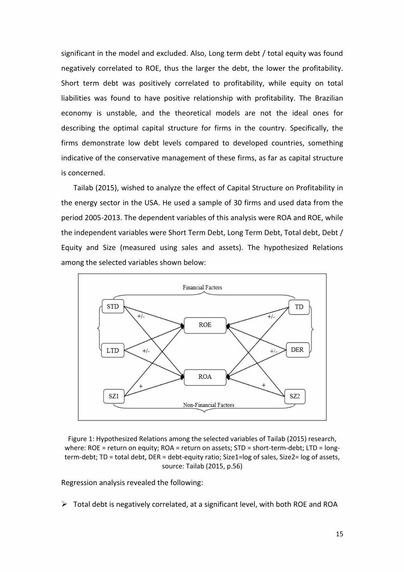
Tailab (2015), wished to analyze the effect of Capital Structure on Profitability in
the energy sector in the USA. He used a sample of 30 firms and used data from the
period 2005-2013. The dependent variables of this analysis were ROA and ROE, while
the independent variables were Short Term Debt, Long Term Debt, Total debt, Debt /
Equity and Size (measured using sales and assets). The hypothesized Relations
among the selected variables shown below:
Figure 1: Hypothesized Relations among the selected variables of Tailab (2015) research, where: ROE = return on equity; ROA = return on assets; STD = short-term-debt; LTD = long-term-debt; TD = total debt, DER = debt-equity ratio; Size1=log of sales, Size2= log of assets,
source: Tailab (2015, p.56)
Regression analysis revealed the following:
Total debt is negatively correlated, at a significant level, with both ROE and ROA
16
Size (measured using sales) harms ROE
Short-term Debt has a significant and positive impact on ROE
Sultan & Adam (2015), investigated the effect of capital structure on profitability
of listed firms in Iraq. The authors argue that capital structure decision, which is
determined by the size and composition of debt and equity, is essential for the
efficient performance and the development of companies because it helps them
become competitive and well-known and, as a result, attract investors. Sultan &
Adam (2015) study’s objectives were the following:
To specify the way capital structure and profitability are correlated
To specify the way capital structure affects profitability evaluation
To reveal the best capital structure choice
The researchers used data from companies listed in the Iraq Stock exchange for
the period 2004 – 2013. The independent variables that they used in their regression
analysis were:
Profit Margin Ratio, which is a performance and profitability ratio and it
demonstrates the net income generated by each monetary unit of sales
Return on Assets Ratio (ROA), which is an efficiency ratio that measures the
effectiveness of using available resources to generate profit
Return on Equity (ROE), which demonstrates the profit generated by equity
Capital structure was measured using the following ratios:
Financial Leverage Ratios (EL), which include Debt Ratio and Debt/Equity Ratio
and demonstrate the percentage of debt a company has, compared to its assets
or equity
Capital Turnover, which is an indicator of the company’s efficiency in using its
capital to generate profit. it is considered a long-term profitability ratio
17
According to Sultan & Adam's (2015) regression analysis results, Capital Structure
positively correlated with profitability and firms should pay attention to create a
capital structure that can make them operate efficiently. Equity is positively
correlated to profitability, while debt negatively correlated to profitability.
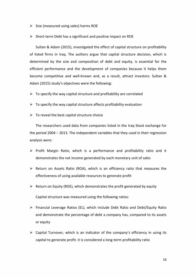
Stekla & Grycova (2015), examined the way capital structure and profitability are
interrelated, and they used data of 706 limited liability companies of the agricultural
sector in the Czech Republic, for the years 2008-2013. They used two ratios to
measure capital structure, Debt to Equity and Debt to Assets. To measure
profitability, the researchers used the following four ratios:
Interest coverage ratio
Gross profit ratio
Net profit ratio
Return on Capital employed
The researchers to test the interrelations of their variables, they developed the
following conceptual model:
Figure 2: Stekla & Grycova (2015) conceptual model, source: Stekla & Grycova (2015, p. 35)
18
According to their research results, there is a negative correlation between Debt
to equity ratio and Debt to Total Asset Ratio and the following ratios:
Return on Capital
Interest Coverage
Net Profit / Gross profit
Stekla & Grycova (2015), research took place during the years of crisis and
revealed that during that period, Debt to assets and Debt to equity ratios were lower
than the recovery period that followed. Also, the variation of profitability ratios is
higher than the variation of the debt ratios.
Hamid et al. (2015), also researched in order to reveal whether a relationship
exists between profitability and capital structure, using data of 46 Family and 46
Non-family firms listed in the Malaysian Stock Exchange, Bursa. The period of the
study was from 2009 to 2011. They used ROE as their dependent variable and
leverage ratios as independent variables (short term debt/total assets, long term
debt/total assets, total debt/total assets). Firm size, Sales growth, and industry type
used as control variables.
According to their research results, ROE for family firms is higher than that of
non-family firms something which demonstrates that family firms are more
profitable. Also, as far as the independent variables are concerned, short term Debt/
Total assets and Total debt/Total assets are higher for family firms, while, on the
other hand, non-family firms seem to finance their operation with long-term debt.
According to the regression analysis results, there is significant negative correlation
between capital structure and profitability, which refers to all independent variables
for both firm categories, except for Short term debt/Total Assets for family firms.
These results are under the pecking order theory, where firms follow a specific
pattern when they wish to finance their activities, and the first use internal funding,
then they use debt and, last, they use equity issuing. On the other hand, results are
not following the trade-off theory, where profitable firms use debt to finance their
activities, something that leads them to further profitability.
19
Mashavave & Tsaurai (2015) used data of firms listed in the Johannesburg Stock
Exchange in South Africa and examined the effect of capital structure on profitability.
The researchers used data for the years 2001 – 2013 and calculated the debt/equity
ratio and profit margin. They found no relationship between capital structure and
profitability for none of the companies of the sample. There were periods where the
ratios were positively correlated and others where they were negatively correlated,
without following a specific pattern. The authors argue that there are external
factors that influence the relationship between capital structure and profitability.
Abeywardhana (2015), investigated the correlation between capital structure
and profitability for SMEs in the United Kingdom, for the years 1998 – 2008. The
study used the dynamic model and used ROA and ROCE (Return on Capital
Employed) as dependent variables, whereas the independent variables of the model
were:
Debt/Assets
Total debt/Total Assets
Long term debt / Total Assets
Short term debt/ Total Assets
Short term Debt / Total Debt
Firm Size, Sales Growth, and Liquidity chosen as control variables. Panel data
analysis revealed a negative correlation between capital structure and profitability
for both the dependent variables. Also, a positive correlation between firm size and
profitability revealed.
Petria et al. (2015) investigated the determinants of profitability in a special
sector, that of banks in the EU27. The European Banking system has encountered a
lot of changes during the last decades, mainly due to European integration, which
took place in several stages, beginning in 1957. The authors use data of 1098
European banks for the period 2001 – 2011. They used Average ROA (ROAA) and
Average ROE (ROAE) as their model’s dependent variables, whereas the independent
variables were:
20
Business Mix Indicator (Other operating Income / Average Bank Assets
Liquidity Risk (Loans / Customer Deposits)
Management Efficiency (Cost / Income Ratio)
Credit Risk (Impaired Loans / Gross Loans
Capital Adequacy (Equity / Total Assets)
Bank Size (Log of Total Assets)
Also, Inflation, Economic Growth, and Market Concentration were the external
factors used in the model. Petria et al. (2015), research results revealed the following
correlations:
ROAE is not affected by the size of the bank, while ROAA is slightly and positively
affected by the size of the bank
Both ROAA and ROAE negatively correlated with the Cost / Income Ratio
Credit Risk is negatively correlated with ROAA and with ROAE, the latter
correlation being stronger
ROAA and ROAE are not significantly affected by Capital Adequacy
Operating Income affects both ROAA and ROAE, with the effect being much
stronger in the case of ROAE
Market concentration reduces profitability; GDP growth is positively correlated
to profitability, while inflation is not significantly correlated to profitability.
Nasimi (2016) used data from British listed companies to investigate the effect
on capital structure on firm profitability. The sample of his study consisted of 30
firms of the top 100 companies that were listed in the FTSE100 Index, in the London
Stock Exchange for the period 2005 – 2014. The researcher developed three
different models, using debt/equity and interest coverage as independent variables
and return on equity (ROE), return on assets (ROA) and return on invested capital
21
(ROIC) as dependent variables. They tested the effect on independent variables in
each of the dependent variables. Their analysis results revealed the following:
There is a positive relationship between Debt/equity and ROE and ROIC
There is a negative relationship between Debt/equity and ROA
Interest Coverage positively correlated with all three independent variables
Debt /equity negatively correlated with Interest Coverage
There is a positive correlation between the independent variables
Vaicondam & Ramakrishnan (2017), examined the effect of capital structure on
profitability for firms that registered in the Malaysian Stock Exchange. They
conducted longitudinal research between the years 2001 and 2014, using 9.912
observations. They used ROA as their dependent variable and long-term debt / total
debt and short-term debt / total debt as independent variables. They found that
short term debt is positively and significantly correlated to ROA, thus to profitability.
On the other hand, long term debt was found to negatively correlated with ROA.
Singh & Bagga (2019) studied Nifty 50 companies listed in the National Stock
Exchange of India, for the period 2008 – 2017, to reveal the effect of Capital
Structure on profitability. Specifically, they used panel data methodology, and ROA
and ROE were the dependent variables of the models they tested, while Total
Liabilities/Total Assets and Total Equity/Total Assets chosen as the independent
variables. Also, Tangibility (Fixed Assets/Total Assets), Tax (EBIT), Business Risk (%
change in EBIT and %change in Net Sales), Liquidity (Current Assets/Current
Liabilities), and Annual Inflation Rate chosen as the models’ control variables.
Singh & Bagga (2019) their regression panel data analysis resulted that there is a
significant impact of Capital structure on profitability, and specifically results
revealed the following:
Random effect model: results show that there is negative correlation between
total Debt and ROA and positive relationship between equity and ROA.

22
Fixed effects model: results reveal a positive correlation between Total Debt and
ROE and a negative correlation between equity and ROE.
After having presented extended literature on the influence of Capital Structure
on Profitability, empirical research follows, to examine, based in above-presented
theory, the impact of capital structure on profitability for companies listed in the
FTSE100 Index as well as companies listed in the FTSE250 Index, in the London Stock
Exchange.
23
4.Research Methodology
4.1 Data
In order to investigate the impact of capital structure on profitability, data of 150
non-financial listed firms were used. Specifically, the author downloaded data via
Thomson-EIKON in the IHU database as well as the London Stock exchange, for the
years 2002-2018. Data referred to 50 companies listed in the FTSE100 Index as well
as 100 companies listed in the FTSE250 Index. Financial firms were not chosen since
the Financial Sector operates with a high proportion of debt, compared to assets, as
a result, these data would not be comparable with other sectors. Furthermore, data
were divided into two sub-periods, the one from 2002 to 2010 and the other from
2011 to 2018. The variables that were included in the analysis are the following:
Dependent Variables:
ROA (Return on Assets)
Return on Assets is calculated using the following type:
ROA = Net Income / Total Assets
It is an efficiency ratio that demonstrates the proportion of profitability in
total assets. In other words, it demonstrates the ability of the company to
generate a profit using its assets.
ROE (Return on Equity)
Return on Equity is calculated using the following type:
ROE = Net Income / Shareholders’ Equity
It is also an efficiency ratio, and, in simple words, it demonstrates the profit a
company generates using each monetary unit of shareholders’ equity. In
other words, it demonstrates the ability of the company to generate profit
using shareholders’ equity.
Gross Profit Margin (%): (Revenue – Cost of Goods Sold) / Revenue
Gross Profit Margin is an indicator of the company’s profit, before costs and
taxes, and it demonstrates how successful the company is in providing
products and services in a profitable way.

24
Independent Variables:
Long-term Debt
Long-term Debt is calculated using the following type:
Long-term Debt / Total Assets
Represents the proportion of the debt the company holds - that has a
maturity of more than twelve months – compared to its total assets
Short-term Debt
Short-term Debt is calculated using the following type:
Short-term Debt / Total Assets
Short-term Debt– or current liabilities – represents the proportion of the
debt that is to be paid within a year, compared to the total assets.
Total Debt
Total Debt is calculated using the following type:
Total Debt / Total Assets
Total Debt consists of Long-Term Debt and Short-Term Debt.
Control Variable:
Sales Growth
Sales Growth was calculated by using the following formula:
(Current Year’s Sales – Previous Year’s Sales) / Previous Year’s Sales
The control variable is used as it has been demonstrated by other researchers who
had also investigated the effect of capital structure on profitability.
4.2 Modeling
The research aims at fulfilling the following objectives:
Identify the nature of the relationship between Capital Structure and Firm
Performance.
Explore the impact of Capital Structure on Firm Performance.
More specifically, the research questions that were developed in order to
fulfil the research objectives are the following:
Is there an impact of Capital structure on ROA?
Is there an impact of Capital Structure on ROE?
25
Is there an impact of Capital Structure on Gross Profit Margin?
4.3 Population
As mentioned above, the research population consists of LSE non-financial
shareholding companies listed in the FTSE100 and FTSE250 in London Stock
Exchange for the study period (2002-2010) and (2011-2018). Specifically, the sample
consists of 50 companies listed in the FTSE 100 (50% of the population) and 100
companies listed in the FTSE 250 (40% of the population).
4.4 Research Hypotheses
To fulfil the research objectives, the following hypotheses were developed:
Model 1:
H0: There is no significant impact of Independent Variables on Return on Asset
H1: There is a significant impact of Independent Variables on Return on Asset.
Model 2:
H0: There is no significant impact of Independent Variables on Return on Equity.
H1: There is significant impact of Independent Variables on Return on Equity.
Model 3:
H0: There is no significant impact of Independent Variables on Gross Profit Margin.
H1: There is significant impact of Independent Variables on Gross Profit Margin.
The above-mentioned hypotheses need to be checked for each of the three
independent variables and for the two periods of investigation (2002-2010 and 2011
– 2018). Also, companies are divided according to the database they are included
(FTSE100 or FTSE250) Thus, 9 different models were developed and regressed,
following the analysis by Abor (2005) and Gill et al. (2011). These models are the
following (which are estimated for the two different periods, 2002-2010 and 2011-
2018 as well as the two groups of companies):
26
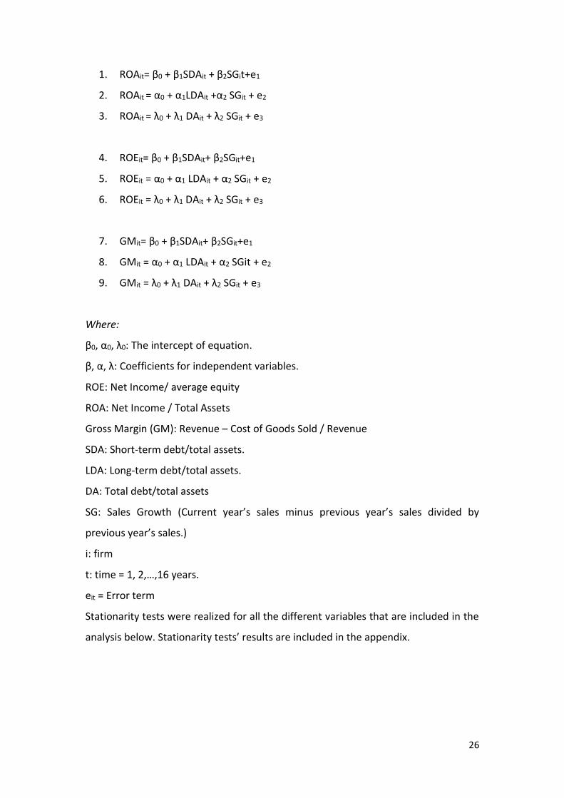
1. ROAit= β0 + β1SDAit + β2SGit+e1
2. ROAit = α0 + α1LDAit +α2 SGit + e2
3. ROAit = λ0 + λ1 DAit + λ2 SGit + e3
4. ROEit= β0 + β1SDAit+ β2SGit+e1
5. ROEit = α0 + α1 LDAit + α2 SGit + e2
6. ROEit = λ0 + λ1 DAit + λ2 SGit + e3
7. GMit= β0 + β1SDAit+ β2SGit+e1
8. GMit = α0 + α1 LDAit + α2 SGit + e2
9. GMit = λ0 + λ1 DAit + λ2 SGit + e3
Where:
β0, α0, λ0: The intercept of equation.
β, α, λ: Coefficients for independent variables.
ROE: Net Income/ average equity
ROA: Net Income / Total Assets
Gross Margin (GM): Revenue – Cost of Goods Sold / Revenue
SDA: Short-term debt/total assets.
LDA: Long-term debt/total assets.
DA: Total debt/total assets
SG: Sales Growth (Current year’s sales minus previous year’s sales divided by
previous year’s sales.)
i: firm
t: time = 1, 2,…,16 years.
eit = Error term
Stationarity tests were realized for all the different variables that are included in the
analysis below. Stationarity tests’ results are included in the appendix.

27
5.Empirical Results & Analysis
5.1 FTSE 100 Period: 2002 – 2010
Results concerning the 50 companies of the FTSE100 Index, for the years 2002-2010
are listed below. The 50 companies of the sample belong to the following sectors:
.
Figure 3: Number of Companies for each Sector FTSE100
Basic Materials, 8%
Consumer Discretionary,
14%
Consumer Staples , 16%
Energy, 8%General
Retailers, 0
Health Care , 6%
Industrials, 34%
Oil Exploration&P
roduction, 0
Real Estate, 4%
Technology, 4% Telecommunications, 4%
Utilities, 2%

28
First descriptive statistics for the variables were calculated and are demonstrated on
table1 below:
Table 1: Descriptive statistics for FTSE100 data for the years 2002-2010
Table 1 demonstrates the descriptive statistics for the variables that are used
for all the models, for the companies that belong to the FTSE Index, for the years
2002 – 2010. It seems that there is important deviation among the Gross Profit
Margins and ROE for the companies of the sample. Nevertheless, the average Gross
Profit Margin as well as ROE is high, something indicative of the effectiveness with
which the companies of the sample were operating during the period 2002 – 2010.
As far as Short-term Debt and Long-term Debt are concerned, there is also
substantial difference between the minimum and maximum values; nevertheless,
standard deviation is not high. It is also important to note that 449 observations
were included.
29
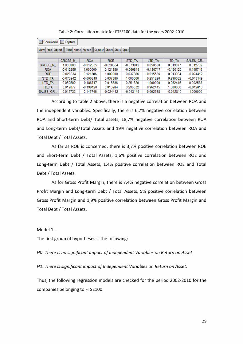
Table 2: Correlation matrix for FTSE100 data for the years 2002-2010
According to table 2 above, there is a negative correlation between ROA and
the independent variables. Specifically, there is 6,7% negative correlation between
ROA and Short-term Debt/ Total assets, 18,7% negative correlation between ROA
and Long-term Debt/Total Assets and 19% negative correlation between ROA and
Total Debt / Total Assets.
As far as ROE is concerned, there is 3,7% positive correlation between ROE
and Short-term Debt / Total Assets, 1,6% positive correlation between ROE and
Long-term Debt / Total Assets, 1,4% positive correlation between ROE and Total
Debt / Total Assets.
As for Gross Profit Margin, there is 7,4% negative correlation between Gross
Profit Margin and Long-term Debt / Total Assets, 5% positive correlation between
Gross Profit Margin and 1,9% positive correlation between Gross Profit Margin and
Total Debt / Total Assets.
Model 1:
The first group of hypotheses is the following:
H0: There is no significant impact of Independent Variables on Return on Asset
H1: There is significant impact of Independent Variables on Return on Asset.
Thus, the following regression models are checked for the period 2002-2010 for the
companies belonging to FTSE100:
30
1.1 ROAit= β0 + β1SDAit+ β2SGit+e1
First, the method OLS was applied to estimate the regression function. The results
are included in the appendix. Short-term Debt is not statistically important in the
95% significance level, something that indicates that there is not significant
correlation between ROA and Short-term Debt, or in other words, there is not
significant impact of Short-term Debt on ROA. The lack of significance is also
indicated by the “t-statistics” value, which demonstrates the statistical importance
of the co-efficient. Also, in this case, t-statistics for Short-term Debt is -1,3, which is
lower than 1,96, thus not statistically important (UCLA, 2015).
Next, the method Fixed Effects (FE) was applied, to obtain better results since
the bias is minimized (the regression is realized for each data group separately).
Results are included in the appendix. According to FE method, Short-term Debt is not
statistically important in the 95% significance level, p=0,06 something that indicates
that there is not significant correlation between ROA and Short-term Debt, or in
other words, there is not significant impact of Short-term Debt on ROA. The lack of
significance is also indicated by the “t-statistics” value, which demonstrates the
statistical importance of the co-efficient. Also, in this case, t-statistics for Short-term
Debt is -1,85, which is lower than 1,96, thus not statistically important (UCLA, 2015).
Then, the Random Effects method was applied. The results of this method, and
specifically the coefficients, take into account the differences among the companies
as well as the differences among the years for a specific company. Thus, results show
the average impact of the independent variable (Short-term Debt) on the dependent
variable (ROA), when the independent variable changes one unit, through time and
among companies. The results are shown in Table 3 below.
31
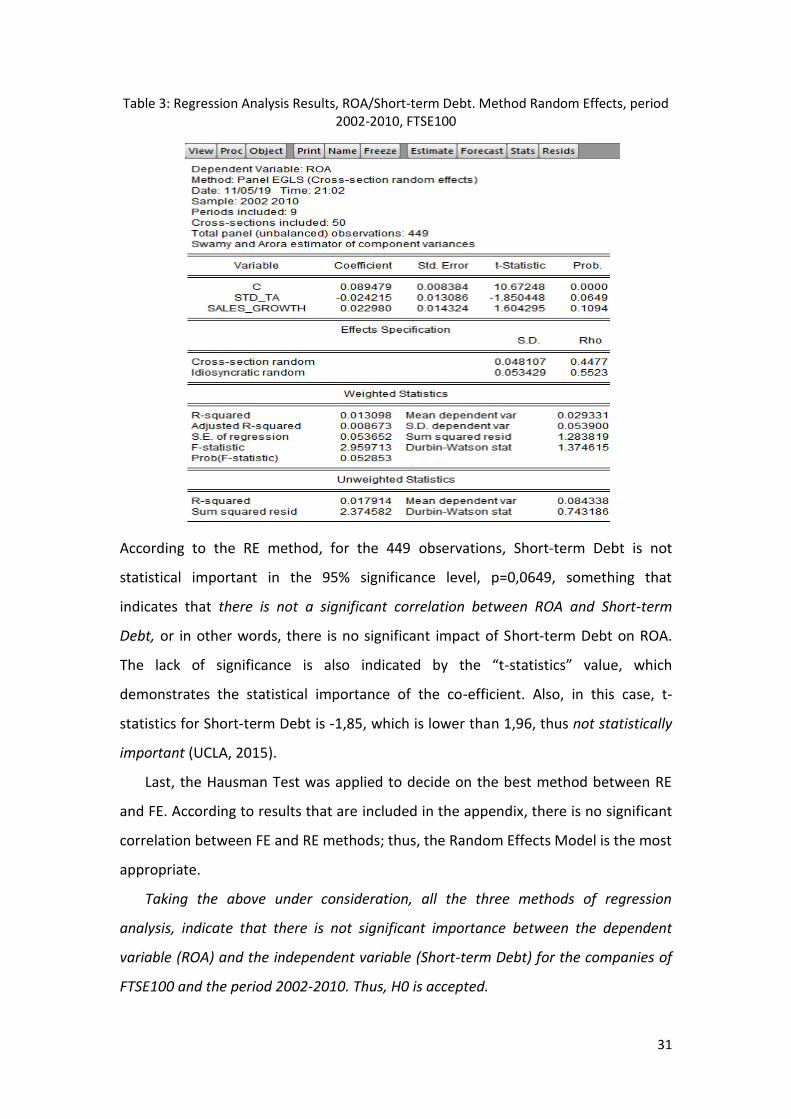
Table 3: Regression Analysis Results, ROA/Short-term Debt. Method Random Effects, period 2002-2010, FTSE100
According to the RE method, for the 449 observations, Short-term Debt is not
statistical important in the 95% significance level, p=0,0649, something that
indicates that there is not a significant correlation between ROA and Short-term
Debt, or in other words, there is no significant impact of Short-term Debt on ROA.
The lack of significance is also indicated by the “t-statistics” value, which
demonstrates the statistical importance of the co-efficient. Also, in this case, t-
statistics for Short-term Debt is -1,85, which is lower than 1,96, thus not statistically
important (UCLA, 2015).
Last, the Hausman Test was applied to decide on the best method between RE
and FE. According to results that are included in the appendix, there is no significant
correlation between FE and RE methods; thus, the Random Effects Model is the most
appropriate.
Taking the above under consideration, all the three methods of regression
analysis, indicate that there is not significant importance between the dependent
variable (ROA) and the independent variable (Short-term Debt) for the companies of
FTSE100 and the period 2002-2010. Thus, H0 is accepted.
32
1.2. ROAit = α0 + α1LDAit +α2 SGit + e2
First, the method OLS was applied in order to estimate the regression function.
Results are shown in appendix. For the 449 observations, Long-term Debt is
statistical important in the 95% significance level, something that indicates that there
is significant correlation between ROA and Long-term Debt, or in other words, there
is significant impact of Long-term Debt on ROA.
Next, the method Fixed Effects (FE) was applied, in order to obtain better results
since the bias is minimized (the regression is realized for each data group
separately). Results are shown in appendix.According to FE method, Long-term Debt
is statistical important in the 95% significance level, p=0,0013, something that
indicates that there is significant correlation between ROA and Long-term Debt, or in
other words, there is significant impact of Long-term Debt on ROA.
Then, the Random Effects method is applied. The results of this method, and
specifically the coefficients, take into account the differences among the companies
as well as the differences among the years for a specific company. Thus, results show
the average impact of the independent variable (Long-term Debt) on the dependent
variable (ROA), when the independent variable changes one unit, through time and
among companies. Results are demonstrated on table 4, below.

33
Table 4: Regression Analysis Results, ROA/Long-term Debt. Method Random Effects, period 2002-2010, FTSE100
According to RE method, for the 449 observations Long-term Debt is statistical
important in the 95% significance level, p=0,0004, something that indicates that
there is significant correlation between ROA and Long-term Debt. The model that can
be developed according to Random Effects Method is the following:
Last, the Hausman Test was applied in order to decide on the best method
between RE and FE. According to results that are shown in appendix, there is not
significant correlation between FE and RE methods; thus, the Random Effects Model
is the most appropriate.
Taking the above under consideration, all the three methods of regression
analysis, indicate that there is significant correlation between the dependent variable
(ROA) and the independent variable (Long-term Debt). Thus, H0 is rejected. Also,
since the RE Method is the most appropriate, the equation that explains the
correlation between the variables is the following:
ROA = 0, 095635 - 0, 060248 LDAit + 0,023671 SGit + e1

34
The equation above shows that 1% increase in Long-term Debt (Ceteris paribus),
results to an average decrease of 6,02% of ROA.
1.3 ROAit = λ0 + λ1 DAit + λ2 SGit + e3
First, the method OLS is applied in order to estimate the regression function. Results
are shown in appendix. For the 449 observations R-squared is 5,7%, something that
indicates that 5,7% of the variation of the dependent variable is explained by the
independent variables. Also, Total Debt is statistical important in the 95%
significance level, p=0,0001, something that indicates that there is significant
correlation between ROA and Total Debt, or in other words, there is significant
impact of Total Debt on ROA. Also, there is negative correlation between the
dependent and the independent variable.
Next, the method Fixed Effects (FE) was applied, in order to obtain better results
since the bias is minimized (the regression is realized for each data group
separately). Results are shown in appendix.According to FE method, Total Debt is
statistical important in the 95% significance level, p=0,0017, something that
indicates that there is significant correlation between ROA and Total Debt.
Then, the Random Effects method is applied. The results of this method, and
specifically the coefficients, take into account the differences among the companies
as well as the differences among the years for a specific company. Thus, results show
the average impact of the independent variable (Total Debt) on the dependent
variable (ROA), when the independent variable changes one unit, through time and
among companies. Results are demonstrated on table 5, below.

35
Table 5: Regression Analysis Results, ROA/Total Debt. Method Random Effects, period 2002-2010, FTSE100
According to RE method, for the 449 observations R-squared is 3,2%, something that
indicates that 3,2% of the variation of the dependent variable is explained by the
independent variables. Also, Total Debt is statistical important in the 95%
significance level, p=0,0005, something that indicates that there is significant
correlation between ROA and Total Debt.
Last, the Hausman Test was applied in order to decide on the best method
between RE and FE. According to results that are shown in appendix, there is not
significant correlation between FE and RE methods; thus, the Random Effects Model
is the most appropriate.
All the three methods of regression analysis indicate that there is significant
correlation between the dependent variable (ROA) and the independent variable
(Total Debt). Thus, H0 is rejected. Also, since the RE Method is the most appropriate,
the equation that explains the correlation between the variables is the following:
ROA = 0, 097357 - 0, 053173 DAit + 0,023260 SGit + e1

36
The equation above shows that 1% increase in Total Debt (Ceteris paribus),
results to an average decrease of 5,3% of ROA.
As far as the first Model is concerned, the regression analysis results revealed
that there is significant negative correlation between ROA and two of the three
independent variables (Long-term Debt and Total Debt).
Model 2:
H0: There is no significant impact of Independent Variables on Return on Equity.
H1: There is significant impact of Independent Variables on Return on Equity.
2.1 ROEit= β0 + β1SDAit+ β2SGit+e1
First, the method OLS is applied in order to estimate the regression function. Results
are shown in appendix. Short-term Debt is not statistical important in the 95%
significance level, something that indicates that there is not significant correlation
between ROE and Short-term Debt, p=0,4424, or in other words, there is not
significant impact of Short-term Debt on ROA.
Next, the method Fixed Effects (FE) was applied, in order to obtain better results
since the bias is minimized (the regression is realized for each data group
separately). Results are shown in appendix. According to FE method, for the 449
observations R-squared is 21,8%, something that indicates that 21,8% of the
variation of the dependent variable is explained by the independent variables. Also,
Short-term Debt is not statistical important in the 95% significance level, p=0,1470,
something that indicates that there is not significant correlation between ROE and
Short-term Debt.
Then, the Random Effects method is applied. The results of this method, and
specifically the coefficients, take into account the differences among the companies
as well as the differences among the years for a specific company. Thus, results show
the average impact of the independent variable (Short-term Debt) on the dependent
variable (ROE), when the independent variable changes one unit, through time and
among companies. Results are demonstrated on table 6, below.

37
Table 6: Regression Analysis Results, ROE/Short-term Debt. Method Random Effects, period 2002-2010, FTSE100
According to RE method, Short-term Debt is not statistical important in the 95%
significance level, p=0,8215, something that indicates that there is not significant
correlation between ROE and Short-term Debt.
Last, the Hausman Test was applied in order to decide on the best method
between RE and FE. According to results that are shown in appendix, there is not
significant correlation between FE and RE methods; thus, the Random Effects Model
is the most appropriate.
Taking the above under consideration, all the three methods of regression
analysis, indicate that there is not significant correlation between the dependent
variable (ROE) and the independent variable (Short-term Debt). Thus, H0 is accepted.
38
2.2 ROEit = α0 + α1 LDAit + α2 SGit + e2
First, the method OLS is applied in order to estimate the regression function. Results
are shown in appendix. For the 449 observations Long-term Debt is not statistical
important in the 95% significance level, p=0,7419, something that indicates that
there is not significant correlation between ROE and Long-term Debt, or in other
words, there is not significant impact of Long-term Debt on ROE.
Next, the method Fixed Effects (FE) was applied, in order to obtain better results
since the bias is minimized (the regression is realized for each data group
separately). Results are shown in appendix. According to FE method, Long-term Debt
is not statistical important in the 95% significance level, p=0,8582, something that
indicates that there is not significant correlation between ROE and Long-term Debt.
Then, the Random Effects method is applied. The results of this method, and
specifically the coefficients, take into account the differences among the companies
as well as the differences among the years for a specific company. Thus, results show
the average impact of the independent variable (Long-term Debt) on the dependent
variable (ROE), when the independent variable changes one unit, through time and
among companies. Results are demonstrated on table7, below.
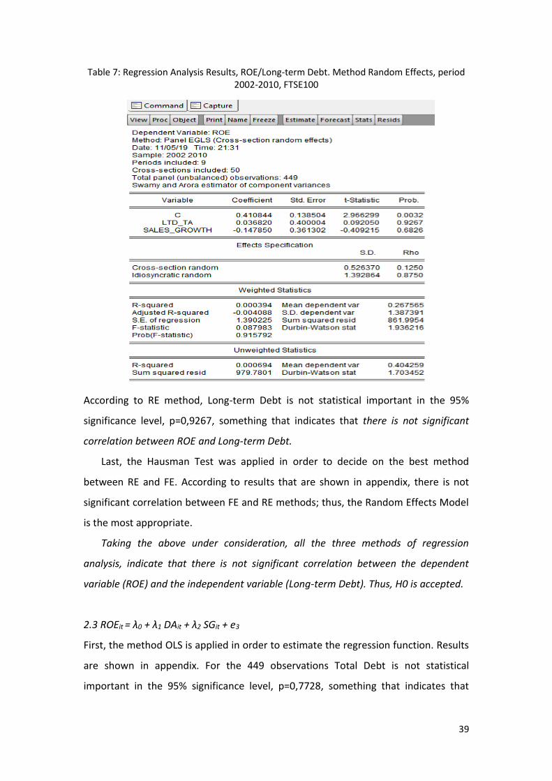
39
Table 7: Regression Analysis Results, ROE/Long-term Debt. Method Random Effects, period 2002-2010, FTSE100
According to RE method, Long-term Debt is not statistical important in the 95%
significance level, p=0,9267, something that indicates that there is not significant
correlation between ROE and Long-term Debt.
Last, the Hausman Test was applied in order to decide on the best method
between RE and FE. According to results that are shown in appendix, there is not
significant correlation between FE and RE methods; thus, the Random Effects Model
is the most appropriate.
Taking the above under consideration, all the three methods of regression
analysis, indicate that there is not significant correlation between the dependent
variable (ROE) and the independent variable (Long-term Debt). Thus, H0 is accepted.
2.3 ROEit = λ0 + λ1 DAit + λ2 SGit + e3
First, the method OLS is applied in order to estimate the regression function. Results
are shown in appendix. For the 449 observations Total Debt is not statistical
important in the 95% significance level, p=0,7728, something that indicates that
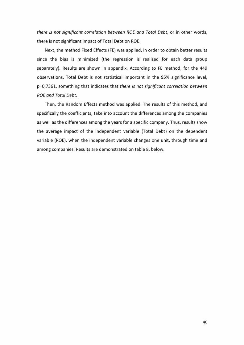
40
there is not significant correlation between ROE and Total Debt, or in other words,
there is not significant impact of Total Debt on ROE.
Next, the method Fixed Effects (FE) was applied, in order to obtain better results
since the bias is minimized (the regression is realized for each data group
separately). Results are shown in appendix. According to FE method, for the 449
observations, Total Debt is not statistical important in the 95% significance level,
p=0,7361, something that indicates that there is not significant correlation between
ROE and Total Debt.
Then, the Random Effects method was applied. The results of this method, and
specifically the coefficients, take into account the differences among the companies
as well as the differences among the years for a specific company. Thus, results show
the average impact of the independent variable (Total Debt) on the dependent
variable (ROE), when the independent variable changes one unit, through time and
among companies. Results are demonstrated on table 8, below.
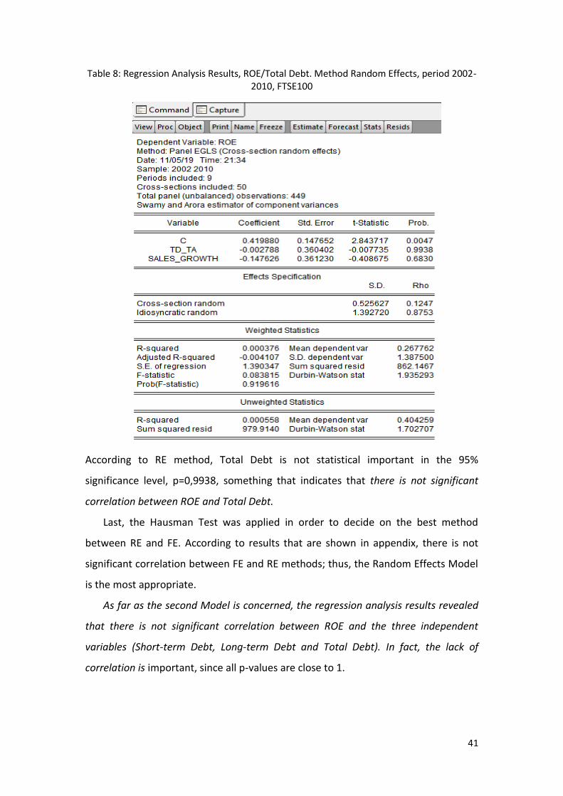
41
Table 8: Regression Analysis Results, ROE/Total Debt. Method Random Effects, period 2002-2010, FTSE100
According to RE method, Total Debt is not statistical important in the 95%
significance level, p=0,9938, something that indicates that there is not significant
correlation between ROE and Total Debt.
Last, the Hausman Test was applied in order to decide on the best method
between RE and FE. According to results that are shown in appendix, there is not
significant correlation between FE and RE methods; thus, the Random Effects Model
is the most appropriate.
As far as the second Model is concerned, the regression analysis results revealed
that there is not significant correlation between ROE and the three independent
variables (Short-term Debt, Long-term Debt and Total Debt). In fact, the lack of
correlation is important, since all p-values are close to 1.
42
Model 3:
H0: There is no significant impact of Independent Variables on Gross Profit Margin
H1: There is significant impact of Independent Variables on Gross Profit Margin
3.1 GMit= β0 + β1SDAit+ β2SGit+e1
First, the method OLS is applied in order to estimate the regression function. Results
are shown in appendix. Short-term Debt is not statistical important in the 95%
significance level, p=0,1205, something that indicates that there is not significant
correlation between Gross Profit Margin and Short-term Debt.
Next, the method Fixed Effects (FE) was applied, in order to obtain better results
since the bias is minimized (the regression is realized for each data group
separately). Results are shown in appendix. According to FE method, Short-term
Debt is not statistical important in the 95% significance level, p=0,9310, something
that indicates that there is not significant correlation between Gross Profit Margin
and Short-term Debt.
Then, the Random Effects method is applied. The results of this method, and
specifically the coefficients, take into account the differences among the companies
as well as the differences among the years for a specific company. Thus, results show
the average impact of the independent variable (Short-term Debt) on the dependent
variable (Gross Profit Margin), when the independent variable changes one unit,
through time and among companies. Results are demonstrated on table9, below.

43
Table 9: Regression Analysis Results, Gross Profit Margin/Short-term Debt. Method Random Effects, period 2002-2010, FTSE100
According to RE method, Short-term Debt is not statistical important in the 95%
significance level, p=0,9045, something that indicates that there is not significant
correlation between Gross Profit Margin and Short-term Debt.
Last, the Hausman Test was applied in order to decide on the best method
between RE and FE. According to results that are shown in appendix, there is not
significant correlation between FE and RE methods; thus, the Random Effects Model
is the most appropriate.
Taking the above under consideration, all the three methods of regression
analysis, indicate that there is not significant correlation between the dependent
variable (Gross Profit Margin) and the independent variable (Short-term Debt). Thus,
H0 is accepted.
44
3.2 GMit = α0 + α1 LDAit + α2 SGit + e2
First, the method OLS is applied in order to estimate the regression function. Results
are shown in appendix. Long-term Debt is not statistical important in the 95%
significance level, p=0,2864, something that indicates that there is not significant
correlation between Gross Profit Margin and Long-term Debt, or in other words,
there is not significant impact of Long-term Debt on Gross Profit Margin.
Next, the method Fixed Effects (FE) was applied. Long-term Debt is not statistical
important in the 95% significance level, p=0,4330, something that indicates that
there is not significant correlation between Gross Profit Margin and Long-term Debt.
Then, the Random Effects method is applied. The results of this method, and
specifically the coefficients, take into account the differences among the companies
as well as the differences among the years for a specific company. Thus, results show
the average impact of the independent variable (Long-term Debt) on the dependent
variable (Gross Profit Margin), when the independent variable changes one unit,
through time and among companies. Results are demonstrated on table 10, below.

45
Table 10: Regression Analysis Results, Gross Margin/Long-term Debt. Method Random Effects, period 2002-2010, FTSE100
According to RE method, Long-term Debt is not statistical important in the 95%
significance level, p=0,3937, something that indicates that there is not significant
correlation between Gross profit Margin and Long-term Debt.
Last, the Hausman Test was applied in order to decide on the best method
between RE and FE. According to results that are shown in appendix, there is not
significant correlation between FE and RE methods; thus, the Random Effects Model
is the most appropriate.
Taking the above under consideration, all the three methods of regression
analysis, indicate that there is not significant correlation between the dependent
variable (Gross Profit Margin) and the independent variable (Long-term Debt). Thus,
H0 is accepted.
3.3 GMit = λ0 + λ1 DAit + λ2 SGit + e3
First, the method OLS is applied in order to estimate the regression function. Results
are shown in appendix. Total Debt is not statistical important in the 95% significance
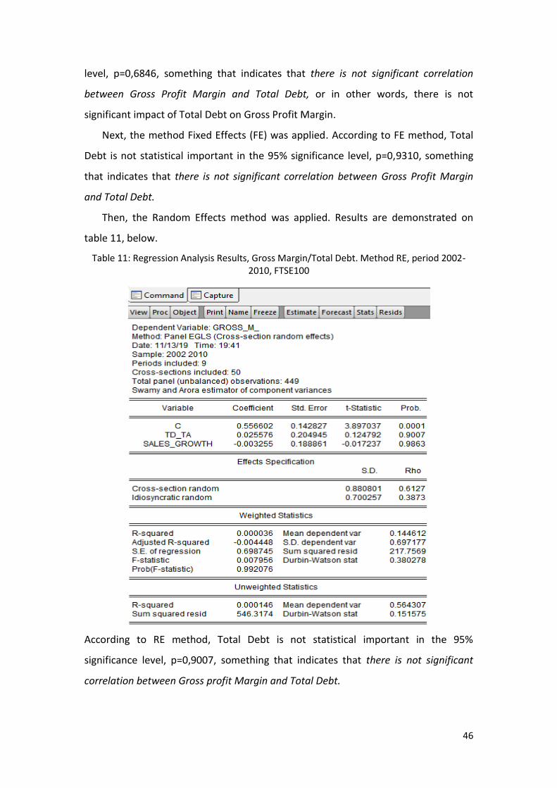
46
level, p=0,6846, something that indicates that there is not significant correlation
between Gross Profit Margin and Total Debt, or in other words, there is not
significant impact of Total Debt on Gross Profit Margin.
Next, the method Fixed Effects (FE) was applied. According to FE method, Total
Debt is not statistical important in the 95% significance level, p=0,9310, something
that indicates that there is not significant correlation between Gross Profit Margin
and Total Debt.
Then, the Random Effects method was applied. Results are demonstrated on
table 11, below.
Table 11: Regression Analysis Results, Gross Margin/Total Debt. Method RE, period 2002-2010, FTSE100
According to RE method, Total Debt is not statistical important in the 95%
significance level, p=0,9007, something that indicates that there is not significant
correlation between Gross profit Margin and Total Debt.
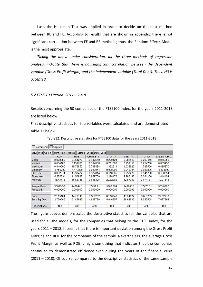
47
Last, the Hausman Test was applied in order to decide on the best method
between RE and FE. According to results that are shown in appendix, there is not
significant correlation between FE and RE methods; thus, the Random Effects Model
is the most appropriate.
Taking the above under consideration, all the three methods of regression
analysis, indicate that there is not significant correlation between the dependent
variable (Gross Profit Margin) and the independent variable (Total Debt). Thus, H0 is
accepted.
5.2 FTSE 100 Period: 2011 – 2018
Results concerning the 50 companies of the FTSE100 Index, for the years 2011-2018
are listed below.
First descriptive statistics for the variables were calculated and are demonstrated in
table 12 below:
Table12: Descriptive statistics for FTSE100 data for the years 2011-2018
The figure above, demonstrates the descriptive statistics for the variables that are
used for all the models, for the companies that belong to the FTSE Index, for the
years 2011 – 2018. It seems that there is important deviation among the Gross Profit
Margins and ROE for the companies of the sample. Nevertheless, the average Gross
Profit Margin as well as ROE is high, something that indicates that the companies
continued to demonstrate efficiency even during the years of the financial crisis
(2011 – 2018). Of course, compared to the descriptive statistics of the same sample
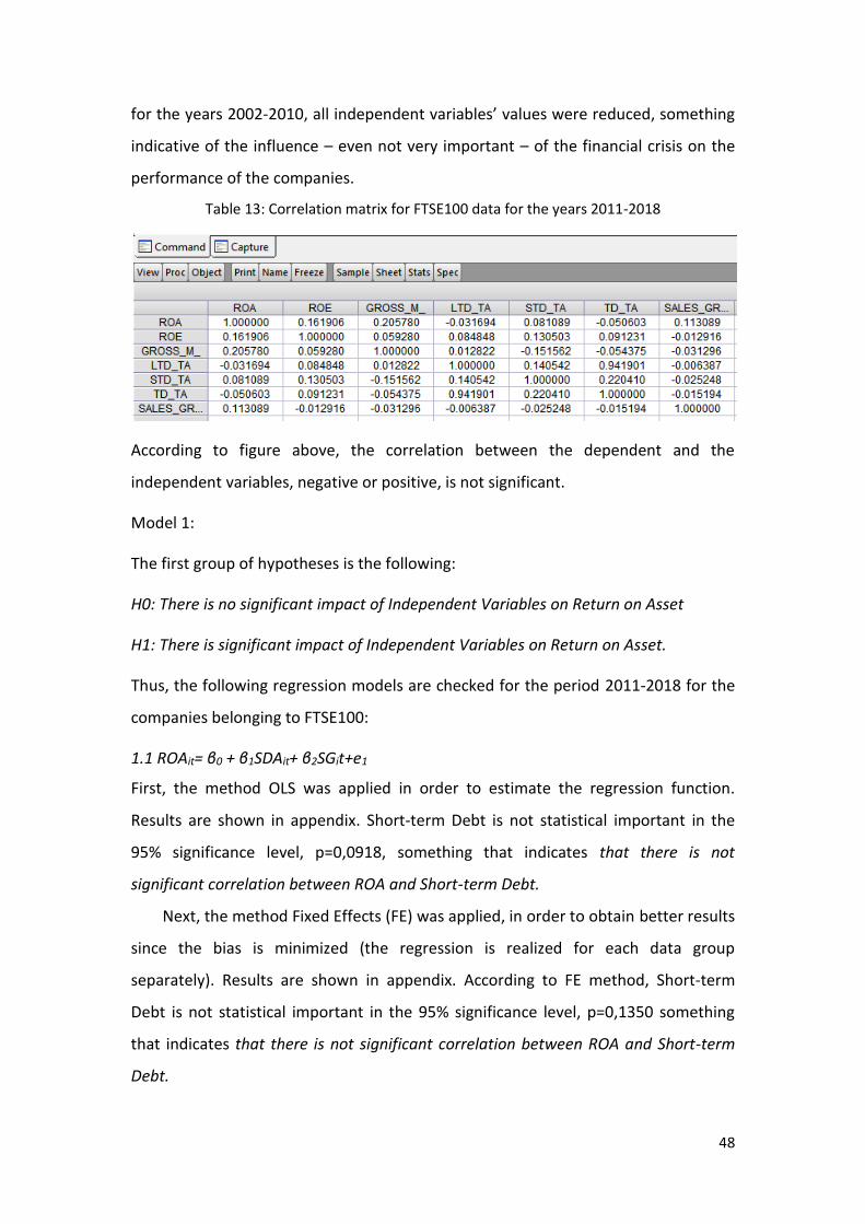
48
for the years 2002-2010, all independent variables’ values were reduced, something
indicative of the influence – even not very important – of the financial crisis on the
performance of the companies.
Table 13: Correlation matrix for FTSE100 data for the years 2011-2018
According to figure above, the correlation between the dependent and the
independent variables, negative or positive, is not significant.
Model 1:
The first group of hypotheses is the following:
H0: There is no significant impact of Independent Variables on Return on Asset
H1: There is significant impact of Independent Variables on Return on Asset.
Thus, the following regression models are checked for the period 2011-2018 for the
companies belonging to FTSE100:
1.1 ROAit= β0 + β1SDAit+ β2SGit+e1
First, the method OLS was applied in order to estimate the regression function.
Results are shown in appendix. Short-term Debt is not statistical important in the
95% significance level, p=0,0918, something that indicates that there is not
significant correlation between ROA and Short-term Debt.
Next, the method Fixed Effects (FE) was applied, in order to obtain better results
since the bias is minimized (the regression is realized for each data group
separately). Results are shown in appendix. According to FE method, Short-term
Debt is not statistical important in the 95% significance level, p=0,1350 something
that indicates that there is not significant correlation between ROA and Short-term
Debt.

49
Then, the Random Effects method is applied. The results of this method, and
specifically the coefficients, take into account the differences among the companies
as well as the differences among the years for a specific company. Thus, results show
the average impact of the independent variable (Short-term Debt) on the dependent
variable (ROA), when the independent variable changes one unit, through time and
among companies. Results are demonstrated on table14, below.
Table 14: Regression Analysis Results, ROA/Short-term Debt. Method Random Effects, period 2011-2018, FTSE100
According to RE method, for the 400 observations Short-term Debt is not statistical
important in the 95% significance level, p=0,0917, something that indicates that
there is not significant correlation between ROA and Short-term Debt.
Last, the Hausman Test was applied in order to decide on the best method
between RE and FE. According to results that are shown in appendix, there is not
significant correlation between FE and RE methods; thus, the Random Effects Model
is the most appropriate.
50
Taking the above under consideration, all the three methods of regression
analysis, indicate that there is not significant importance between the dependent
variable (ROA) and the independent variable (Short-term Debt) for the companies of
FTSE100 and for the period 2011-2018. Thus, H0 is accepted.
1.2. ROAit = α0 + α1 LDAit + α2 SGit + e2
First, the method OLS was applied in order to estimate the regression function.
Results are shown in appendix. Long-term Debt is not statistical important in the
95% significance level, something that indicates that there is not significant
correlation between ROA and Long-term Debt.
Next, the method Fixed Effects (FE) was applied, in order to obtain better results
since the bias is minimized (the regression is realized for each data group
separately). Results are shown in appendix. For the 400 observations, Long-term
Debt is not statistical important in the 95% significance level, p=0,5348, something
that indicates that there is not significant correlation between ROA and Long-term
Debt.
Then, the Random Effects method is applied. The results of this method, and
specifically the coefficients, take into account the differences among the companies
as well as the differences among the years for a specific company. Thus, results show
the average impact of the independent variable (Long-term Debt) on the dependent
variable (ROA), when the independent variable changes one unit, through time and
among companies. Results are demonstrated on table15, below.

51
Table15: Regression Analysis Results, ROA/Long-term Debt. Method Random Effects, period 2011-2018, FTSE100
According to RE method, for the 400 observations, Long-term Debt is not statistical
important in the 95% significance level, p=0,5344, something that indicates that
there is not significant correlation between ROA and Long-term Debt.
Last, the Hausman Test was applied in order to decide on the best method
between RE and FE. According to results that are shown in appendix, there is not
significant correlation between FE and RE methods; thus, the Random Effects Model
is the most appropriate.
Taking the above under consideration, all the three methods of regression
analysis, indicate that there is not significant correlation between the dependent
variable (ROA) and the independent variable (Long-term Debt). Thus, H0 is accepted.
52
1.3 ROAit = λ0 + λ1 DAit + λ2 SGit + e3
First, the method OLS is applied in order to estimate the regression function. Results
are shown in appendix. Total Debt is not statistical important in the 95% significance
level, p=0,3269, something that indicates that there is not significant correlation
between ROA and Total Debt.
Next, the method Fixed Effects (FE) was applied, in order to obtain better results
since the bias is minimized (the regression is realized for each data group
separately). Results are shown in appendix. According to FE method, Total Debt is
not statistical important in the 95% significance level, p=0,3104, something that
indicates that there is not significant correlation between ROA and Total Debt.
Then, the Random Effects method is applied. The results of this method, and
specifically the coefficients, take into account the differences among the companies
as well as the differences among the years for a specific company. Thus, results show
the average impact of the independent variable (Total Debt) on the dependent
variable (ROA), when the independent variable changes one unit, through time and
among companies. Results are demonstrated on table16, below.
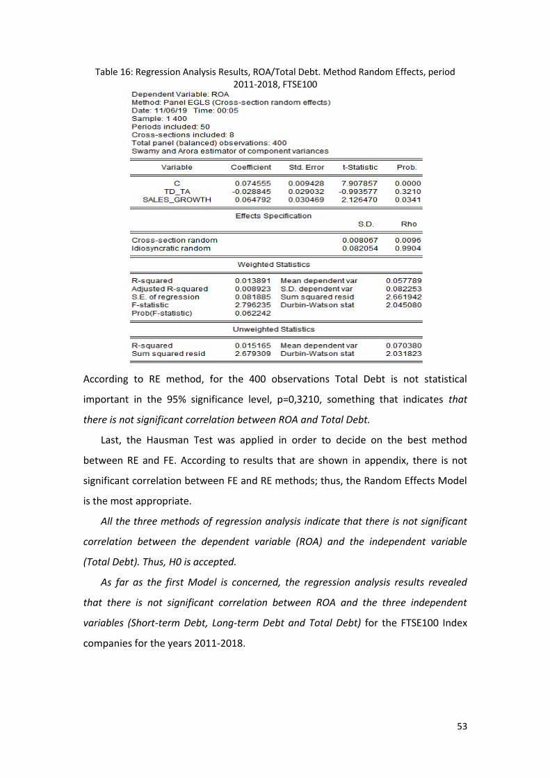
53
Table 16: Regression Analysis Results, ROA/Total Debt. Method Random Effects, period 2011-2018, FTSE100
According to RE method, for the 400 observations Total Debt is not statistical
important in the 95% significance level, p=0,3210, something that indicates that
there is not significant correlation between ROA and Total Debt.
Last, the Hausman Test was applied in order to decide on the best method
between RE and FE. According to results that are shown in appendix, there is not
significant correlation between FE and RE methods; thus, the Random Effects Model
is the most appropriate.
All the three methods of regression analysis indicate that there is not significant
correlation between the dependent variable (ROA) and the independent variable
(Total Debt). Thus, H0 is accepted.
As far as the first Model is concerned, the regression analysis results revealed
that there is not significant correlation between ROA and the three independent
variables (Short-term Debt, Long-term Debt and Total Debt) for the FTSE100 Index
companies for the years 2011-2018.
54
Model 2:
H0: There is no significant impact of Independent Variables on Return on Equity.
H1: There is significant impact of Independent Variables on Return on Equity.
2.1 ROEit= β0 + β1SDAit+ β2SGit+e1
First, the method OLS was applied in order to estimate the regression function.
Results are shown in appendix. Short-term Debt is statistical important in the 95%
significance level, p=0,0092, something that indicates that there is significant
correlation between ROE and Short-term Debt, or in other words, there is significant
impact of Short-term Debt on ROA.
Next, the method Fixed Effects (FE) was applied, in order to obtain better results
since the bias is minimized (the regression is realized for each data group
separately). Results are shown in appendix. According to FE method, Short-term
Debt is statistical important in the 95% significance level, p=0,0069, something that
indicates that there is significant correlation between ROE and Short-term Debt.
Then, the Random Effects method is applied. The results of this method, and
specifically the coefficients, take into account the differences among the companies
as well as the differences among the years for a specific company. Thus, results show
the average impact of the independent variable (Short-term Debt) on the dependent
variable (ROE), when the independent variable changes one unit, through time and
among companies. Results are demonstrated on table 17, below.

55
Table 17: Regression Analysis Results, ROE/Short-term Debt. Method Random Effects, period 2011-2018, FTSE100
According to RE method, for the 400 observations Short-term Debt is statistically
important in the 95% significance level, p=0,0094, something that indicates that
there is significant correlation between ROE and Short-term Debt.
Last, the Hausman Test was applied in order to decide on the best method
between RE and FE. According to results that are shown in appendix, there is not
significant correlation between FE and RE methods; thus, the Random Effects Model
is the most appropriate.
Taking the above under consideration, all the three methods of regression
analysis, indicate that there is not significant correlation between the dependent
variable (ROE) and the independent variable (Short-term Debt). Thus, H0 is accepted.
Also, since the RE method is the most appropriate the model that is derived by the
regression analysis is the following:
ROE = 0,191935 + 0,624611 SDAit - 0,086181 SGit + e1
56
The equation above shows that there is positive correlation between the
variables and that 1% increase in Short-term Debt (Ceteris paribus), results to an
average increase of 62,5% of ROE.
2.2 ROEit = α0 + α1 LDAit + α2 SGit + e2
First, the method OLS was applied in order to estimate the regression function.
Results are shown in appendix. For the 400 observations Long-term Debt is not
statistical important in the 95% significance level, p=0,0908, but it is statistically
important in the 90% significance level. Something that indicates that there is
significant correlation between ROE and Long-term Debt, or in other words, there is
significant impact of Long-term Debt on ROE. The regression is the following:
ROEit = 0,175859 + 0,882476 LDAit – 0,110775 SGit + e2
Next, the method Fixed Effects (FE) was applied, in order to obtain better results
since the bias is minimized (the regression is realized for each data group
separately). Results are shown in appendix. According to FE method, of which the
results are shown on figure above, Long-term Debt is not statistical important in the
95% significance level, p=0,1110, something that indicates that there is not
significant correlation between ROE and Long-term Debt.
Then, the Random Effects method is applied. The results of this method, and
specifically the coefficients, take into account the differences among the companies
as well as the differences among the years for a specific company. Thus, results show
the average impact of the independent variable (Long-term Debt) on the dependent
variable (ROE), when the independent variable changes one unit, through time and
among companies. Results are demonstrated on Table 18, below.
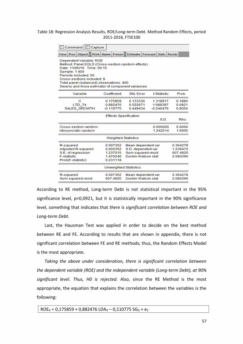
57
Table 18: Regression Analysis Results, ROE/Long-term Debt. Method Random Effects, period 2011-2018, FTSE100
According to RE method, Long-term Debt is not statistical important in the 95%
significance level, p=0,0921, but it is statistically important in the 90% significance
level, something that indicates that there is significant correlation between ROE and
Long-term Debt.
Last, the Hausman Test was applied in order to decide on the best method
between RE and FE. According to results that are shown in appendix, there is not
significant correlation between FE and RE methods; thus, the Random Effects Model
is the most appropriate.
Taking the above under consideration, there is significant correlation between
the dependent variable (ROE) and the independent variable (Long-term Debt), at 90%
significant level. Thus, H0 is rejected. Also, since the RE Method is the most
appropriate, the equation that explains the correlation between the variables is the
following:
ROEit = 0,175859 + 0,882476 LDAit – 0,110775 SGit + e2
58
The equation above shows that there is positive correlation between the variables
and that 1% increase in Long-term Debt (Ceteris paribus), results to an average
increase of 88,25% of ROE.
2.3 ROEit = λ0 + λ1 DAit + λ2 SGit + e3
First, the method OLS is applied in order to estimate the regression function. Results
are shown in appendix. Total Debt is not statistically important in the 95%
significance level, p=0,0692, but it is statistically important in at 90% significance
level, something that indicates that there is significant correlation between ROE and
Total Debt.
Next, the method Fixed Effects (FE) was applied, in order to obtain better results
since the bias is minimized (the regression is realized for each data group
separately). Results are shown in appendix.
According to FE method, of which the results are shown on figure above, Total
Debt is not statistically important in the 95% significance level, p=0,0811, but it is
statistically important in at 90% significance level, something that indicates that
there is significant correlation between ROE and Total Debt.
Then, the Random Effects method is applied. The results of this method, and
specifically the coefficients, take into account the differences among the companies
as well as the differences among the years for a specific company. Thus, results show
the average impact of the independent variable (Total Debt) on the dependent
variable (ROE), when the independent variable changes one unit, through time and
among companies. Results are demonstrated on table 19, below.

59
Table 19: Regression Analysis Results, ROE/Total Debt. Method Random Effects, period 2011-2018, FTSE100
According to RE method, Total Debt is not statistical important in the 95%
significance level, p=0,0703, but it is statistically important in the 90% significance
level. something that indicates that there is significant correlation between ROE and
Total Debt.
Last, the Hausman Test was applied in order to decide on the best method
between RE and FE. According to results that are shown in appendix, there is not
significant correlation between FE and RE methods; thus, the Random Effects Model
is the most appropriate.
Taking the above under consideration, there is significant correlation between
the dependent variable (ROE) and the independent variable (Total Debt), at 90%
significant level. Thus, H0 is rejected. Also, since the RE Method is the most
appropriate, the equation that explains the correlation between the variables is the
following:
ROEit = 0,156472 + 0,795286 DAit – 0,103236 SGit + e2
The equation above shows that there is positive correlation between the
variables and that 1% increase in Total Debt (Ceteris paribus), results to an average
increase of 79,53% of ROE.
60
As far as the second Model is concerned, the regression analysis results revealed
that there is significant correlation between ROE and the three independent variables
(Short-term Debt, Long-term Debt and Total Debt), at the 95% and the 90%
significance level.
Model 3:
H0: There is no significant impact of Independent Variables on Gross Profit Margin
H1: There is significant impact of Independent Variables on Gross Profit Margin
3.1 GMit= β0 + β1SDAit+ β2SGit+e1
First, the method OLS was applied in order to estimate the regression function.
Results are shown in appendix. According to figure above, Short-term Debt is
statistically important in the 95% significance level, p=0,0023, something that
indicates that there is significant negative correlation between Gross Profit Margin
and Short-term Debt.
Next, the method Fixed Effects (FE) was applied, in order to obtain better results
since the bias is minimized (the regression is realized for each data group
separately). Results are shown in appendix. According to FE method, for the 400
observations, Short-term Debt is statistically important in the 95% significance level,
p=0,0019, something that indicates that there is significant correlation between
Gross Profit Margin and Short-term Debt.
Then, the Random Effects method is applied. The results of this method, and
specifically the coefficients, take into account the differences among the companies
as well as the differences among the years for a specific company. Thus, results show
the average impact of the independent variable (Short-term Debt) on the dependent
variable (Gross Profit Margin), when the independent variable changes one unit,
through time and among companies. Results are demonstrated on table20, below.
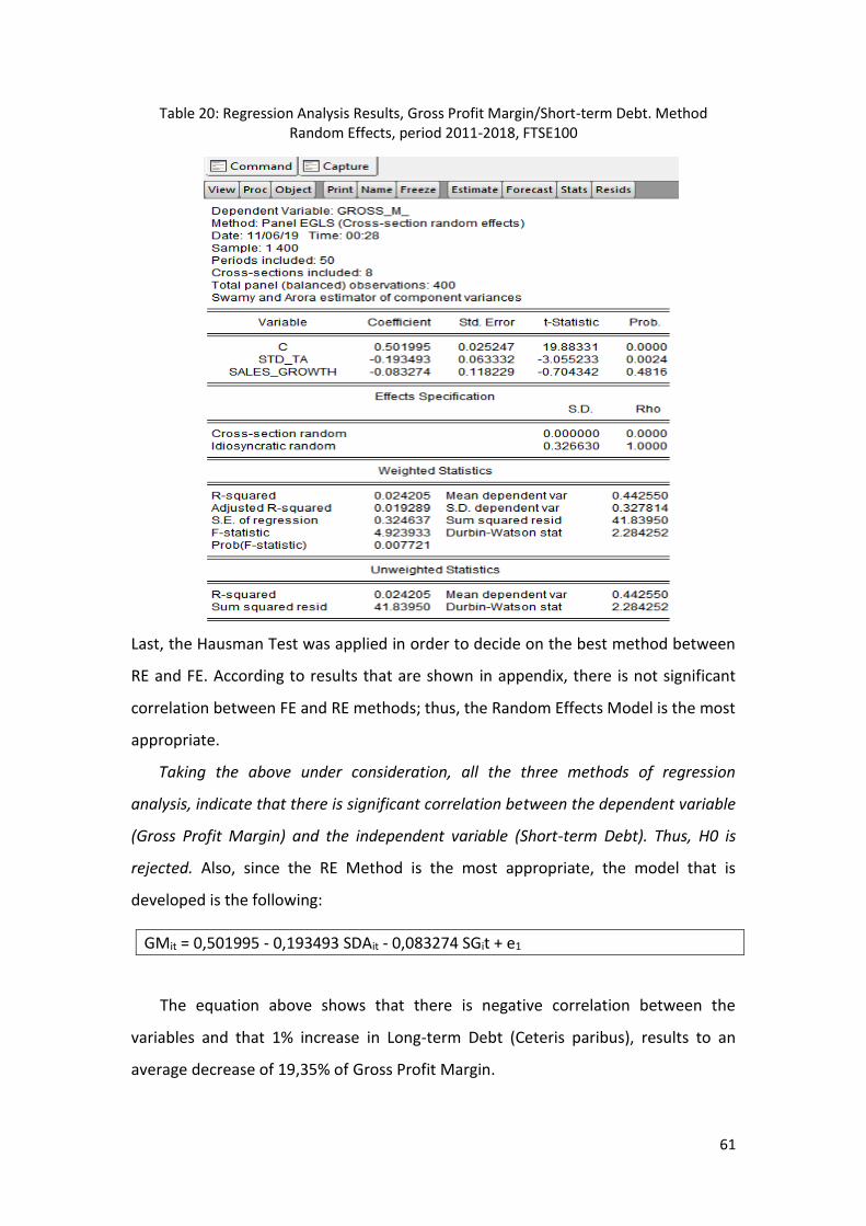
61
Table 20: Regression Analysis Results, Gross Profit Margin/Short-term Debt. Method Random Effects, period 2011-2018, FTSE100
Last, the Hausman Test was applied in order to decide on the best method between
RE and FE. According to results that are shown in appendix, there is not significant
correlation between FE and RE methods; thus, the Random Effects Model is the most
appropriate.
Taking the above under consideration, all the three methods of regression
analysis, indicate that there is significant correlation between the dependent variable
(Gross Profit Margin) and the independent variable (Short-term Debt). Thus, H0 is
rejected. Also, since the RE Method is the most appropriate, the model that is
developed is the following:
GMit = 0,501995 - 0,193493 SDAit - 0,083274 SGit + e1
The equation above shows that there is negative correlation between the
variables and that 1% increase in Long-term Debt (Ceteris paribus), results to an
average decrease of 19,35% of Gross Profit Margin.

62
3.2 GMit = α0 + α1 LDAit + α2 SGit + e2
First, the method OLS is applied in order to estimate the regression function. Results are shown in appendix. For the 400 observations Long-term Debt is not statistical important in the 95% significance level, p=0,8014, something that indicates that there is not significant correlation between Gross Profit Margin and Long-term Debt, or in other words, there is not significant impact of Long-term Debt on Gross Profit Margin.
Next, the method Fixed Effects (FE) was applied, in order to obtain better results since the bias is minimized (the regression is realized for each data group separately). Results are shown in appendix. According to FE method, Long-term Debt is not statistical important in the 95% significance level, p=0,7717, something that indicates that there is not significant correlation between Gross Profit Margin and Long-term Debt.
Then, the Random Effects method is applied. The results of this method, and specifically the coefficients, take into account the differences among the companies as well as the differences among the years for a specific company. Thus, results show the average impact of the independent variable (Long-term Debt) on the dependent variable (Gross Profit Margin), when the independent variable changes one unit, through time and among companies. Results are demonstrated on table 21, below.
Table 21: Regression Analysis Results, Gross Profit Margin/Long-term Debt. Method Random Effects, period 2011-2018, FTSE100

63
According to RE method, Long-term Debt is not statistical important in the 95%
significance level, p=0,8028, something that indicates that there is not significant
correlation between Gross Profit Margin and Long-term Debt.
Last, the Hausman Test was applied in order to decide on the best method
between RE and FE. According to results that are shown in appendix, there is not
significant correlation between FE and RE methods; thus, the Random Effects Model
is the most appropriate.
Taking the above under consideration, all the three methods of regression
analysis, indicate that there is not significant correlation between the dependent
variable (Gross Profit Margin) and the independent variable (Long-term Debt). Thus,
H0 is accepted.
3.3 GMit = λ0 + λ1 DAit + λ2 SGit + e3
First, the method OLS is applied in order to estimate the regression function. Results
are shown in appendix. Total Debt is not statistical important in the 95% significance
level, p=0,2741, something that indicates that there is not significant correlation
between Gross Profit Margin and Total Debt.
Next, the method Fixed Effects (FE) was applied, in order to obtain better results
since the bias is minimized (the regression is realized for each data group
separately). Results are shown in appendix.
According to FE method, Total Debt is not statistically important in the 95%
significance level, p=0,2803, something that indicates that there is not significant
correlation between Gross Profit Margin and Total Debt.
Then, the Random Effects method is applied. The results of this method, and
specifically the coefficients, take into account the differences among the companies
as well as the differences among the years for a specific company. Thus, results show
the average impact of the independent variable (Total Debt) on the dependent
variable (Gross Profit Margin), when the independent variable changes one unit,
through time and among companies. Results are demonstrated on table 22, below.
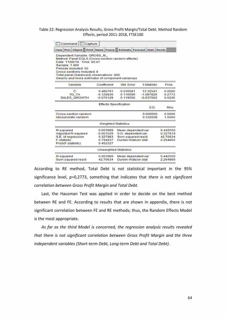
64
Table 22: Regression Analysis Results, Gross Profit Margin/Total Debt. Method Random Effects, period 2011-2018, FTSE100
According to RE method, Total Debt is not statistical important in the 95%
significance level, p=0,2773, something that indicates that there is not significant
correlation between Gross Profit Margin and Total Debt.
Last, the Hausman Test was applied in order to decide on the best method
between RE and FE. According to results that are shown in appendix, there is not
significant correlation between FE and RE methods; thus, the Random Effects Model
is the most appropriate.
As far as the third Model is concerned, the regression analysis results revealed
that there is not significant correlation between Gross Profit Margin and the three
independent variables (Short-term Debt, Long-term Debt and Total Debt).
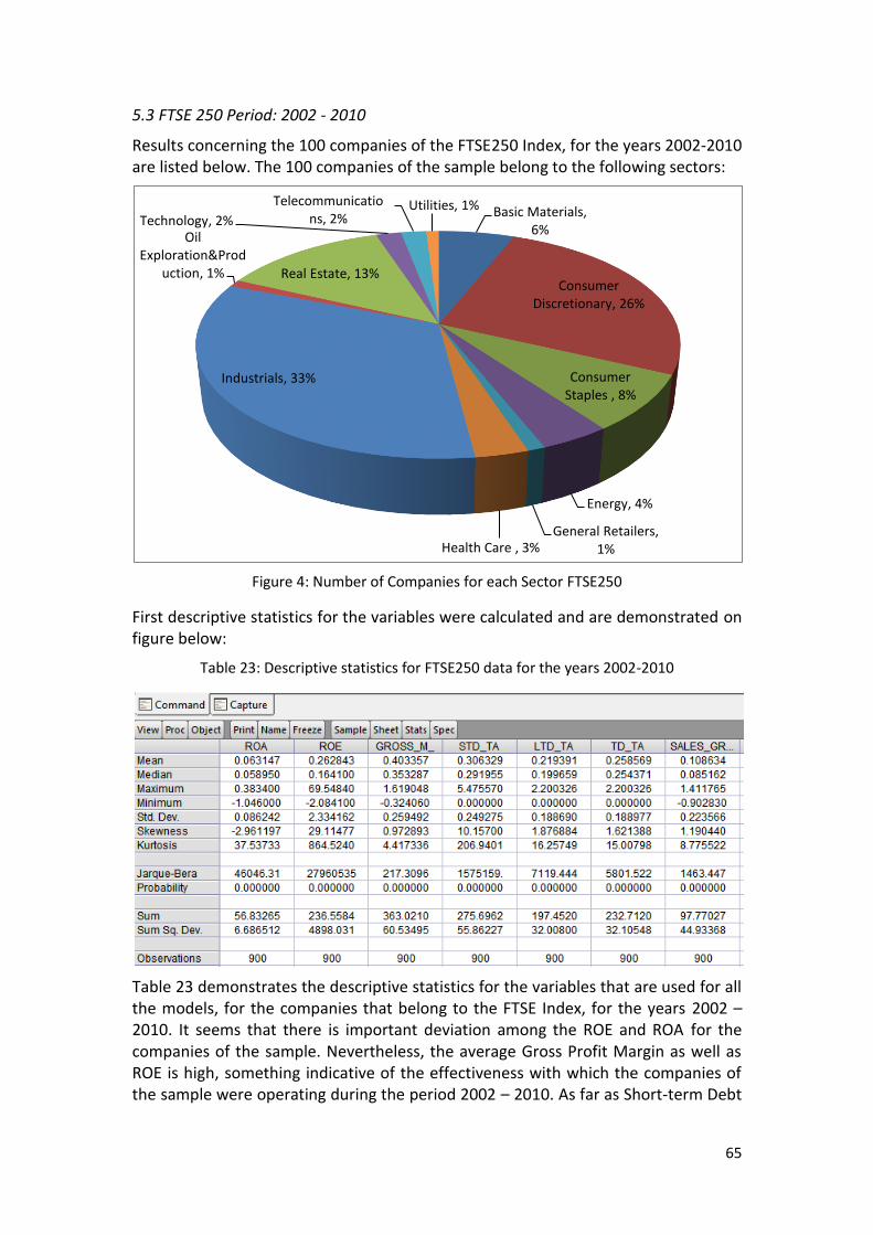
65
5.3 FTSE 250 Period: 2002 - 2010
Results concerning the 100 companies of the FTSE250 Index, for the years 2002-2010 are listed below. The 100 companies of the sample belong to the following sectors:
Figure 4: Number of Companies for each Sector FTSE250
First descriptive statistics for the variables were calculated and are demonstrated on figure below:
Table 23: Descriptive statistics for FTSE250 data for the years 2002-2010
Table 23 demonstrates the descriptive statistics for the variables that are used for all the models, for the companies that belong to the FTSE Index, for the years 2002 – 2010. It seems that there is important deviation among the ROE and ROA for the companies of the sample. Nevertheless, the average Gross Profit Margin as well as ROE is high, something indicative of the effectiveness with which the companies of the sample were operating during the period 2002 – 2010. As far as Short-term Debt
Basic Materials, 6%
Consumer Discretionary, 26%
Consumer Staples , 8%
Energy, 4%
General Retailers, 1%Health Care , 3%
Industrials, 33%
Oil Exploration&Prod
uction, 1% Real Estate, 13%
Technology, 2%
Telecommunications, 2%
Utilities, 1%
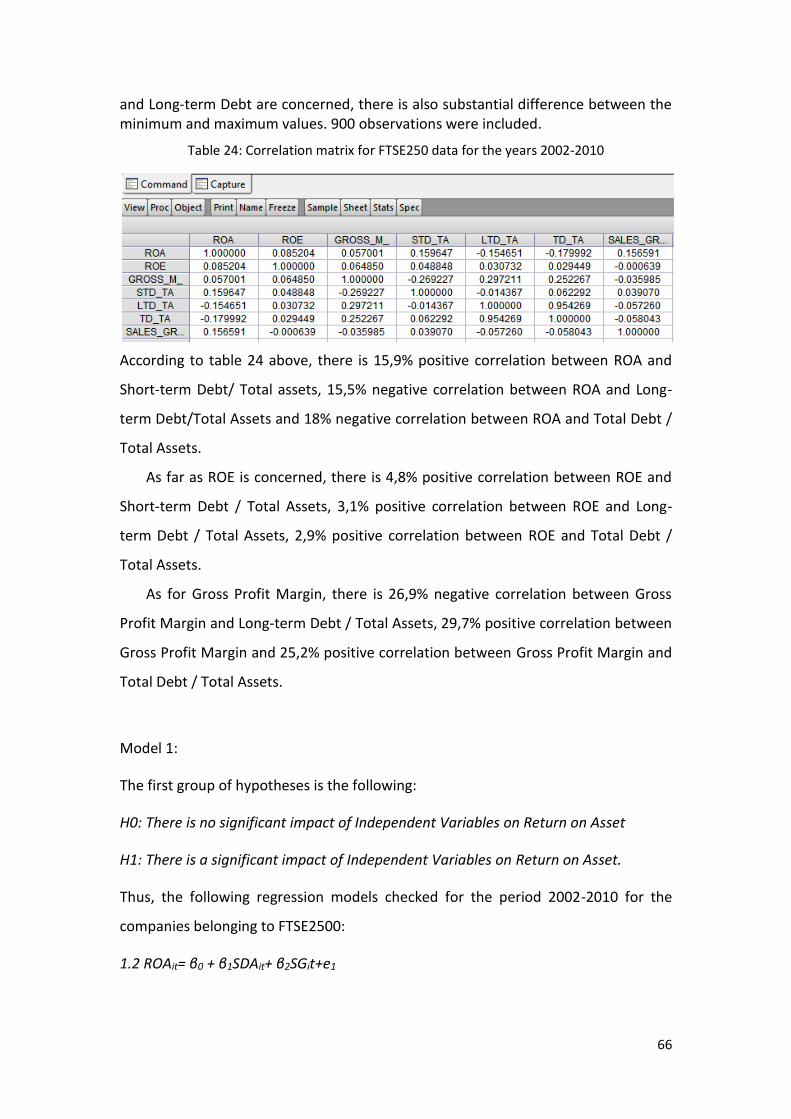
66
and Long-term Debt are concerned, there is also substantial difference between the minimum and maximum values. 900 observations were included.
Table 24: Correlation matrix for FTSE250 data for the years 2002-2010
According to table 24 above, there is 15,9% positive correlation between ROA and
Short-term Debt/ Total assets, 15,5% negative correlation between ROA and Long-
term Debt/Total Assets and 18% negative correlation between ROA and Total Debt /
Total Assets.
As far as ROE is concerned, there is 4,8% positive correlation between ROE and
Short-term Debt / Total Assets, 3,1% positive correlation between ROE and Long-
term Debt / Total Assets, 2,9% positive correlation between ROE and Total Debt /
Total Assets.
As for Gross Profit Margin, there is 26,9% negative correlation between Gross
Profit Margin and Long-term Debt / Total Assets, 29,7% positive correlation between
Gross Profit Margin and 25,2% positive correlation between Gross Profit Margin and
Total Debt / Total Assets.
Model 1:
The first group of hypotheses is the following:
H0: There is no significant impact of Independent Variables on Return on Asset
H1: There is a significant impact of Independent Variables on Return on Asset.
Thus, the following regression models checked for the period 2002-2010 for the
companies belonging to FTSE2500:
1.2 ROAit= β0 + β1SDAit+ β2SGit+e1

67
First, the method OLS was applied. The results included in the appendix. Short-term
Debt is statistically important in the 95% significance level, p=0,00, something that
indicates that there is a significant correlation between ROA and Short-term Debt.
Next, the method Fixed Effects (FE) was applied, to obtain better results since
the bias is minimized (the regression is realized for each data group separately). The
results are included in the appendix. According to FE method, Short-term Debt is
statistically important in the 95% significance level, p=0,04, something that indicates
that there is a significant correlation between ROA and Short-term Debt, or in other
words, there is not the significant impact of Short-term Debt on ROA.
Then, the Random Effects method was applied. The results of this method, and
specifically the coefficients, take into account the differences among the companies
as well as the differences among the years for a specific company. Thus, results show
the average impact of the independent variable (Short-term Debt) on the dependent
variable (ROA), when the independent variable changes one unit, through time and
among companies. Results are shown on table25, below.

68
Table 25: Regression Analysis Results, ROA/Short-term Debt. Method Random Effects, period 2002-2010, FTSE250
According to RE method, for the 900 observations, Short-term Debt is not statistical
important in the 95% significance level, p=0,00, something that indicates that there
is a significant correlation between ROA and Short-term Debt.
Last, the Hausman test applied in order to decide on the best method between
RE and FE. According to results that included in the appendix, there is not a
significant correlation between FE and RE methods; thus, the Random Effects Model
is the most appropriate.
Taking the above under consideration, all the three methods of regression
analysis, indicate that there is significant importance between the dependent
variable (ROA) and the independent variable (Short-term Debt) for the companies of
FTSE250 and for the period 2002-2010. Thus, H0 is rejected. The model developed is
the following:

69
ROAit= 0,044403 + 0,042990 SDAit+ 0,051320 SGit+e1
The equation above shows that there is positive correlation between the
variables and that 1% increase in Short-term Debt (Ceteris paribus), results to an
average decrease of 4,3% of ROA.
1.2. ROAit = α0 + α1 LDAit + α2 SGit + e2
First, the method OLS applied to estimate the regression function. The results are
shown in the appendix. Long-term Debt is statistical important in the 95%
significance level, p=0,00, something that indicates that there is a significant
correlation between ROA and Long-term Debt, or in other words, there is a
significant impact of Long-term Debt on ROA.
Next, the method Fixed Effects (FE) was applied, in order to obtain better results
since the bias is minimized (the regression is realized for each data group
separately). The results are shown in the appendix. According to FE method, Long-
term Debt is statistical important in the 95% significance level, p=0,00, something
that indicates that there is significant correlation between ROA and Long-term Debt,
or in other words, there is significant impact of Long-term Debt on ROA.
Then, the Random Effects method is applied. The results of this method, and
specifically the coefficients, take into account the differences among the companies
as well as the differences among the years for a specific company. Thus, results show
the average impact of the independent variable (Long-term Debt) on the dependent
variable (ROA), when the independent variable changes one unit, through time and
among companies. Results are demonstrated on table 26, below.

70
Table 26: Regression Analysis Results, ROA/Long-term Debt. Method Random Effects, period 2002-2010, FTSE250
According to RE method, for the 900 observations Long-term Debt is statistical
important in the 95% significance level, p=0,00, something that indicates that there
is a significant correlation between ROA and Long-term Debt.
Last, the Hausman Test applied to decide on the best method between RE and
FE. According to results that are shown in the appendix, there is no significant
correlation between FE and RE methods; thus, the Random Effects Model is the most
appropriate.
Taking the above under consideration, all three methods of regression analysis
indicate that there is a significant correlation between the dependent variable (ROA)
and the independent variable (Long-term Debt). Thus, H0 rejected. Also, since the RE
Method is the most appropriate, the equation that explains the correlation between
the variables is the following:

71
ROA = 0, 073044 - 0, 071040 LDAit + 0,052365 SGit + e1
The equation above shows that 1% increase in Long-term Debt (Ceteris paribus)
results in an average decrease of 7,1% of ROA.
1.3 ROAit = λ0 + λ1 DAit + λ2 SGit + e3
First, the method OLS is applied in order to estimate the regression function. The
results are shown in the appendix. For the 900 observations, Total Debt is statistical
important in the 95% significance level, p=0,00, something that indicates that there
is a significant correlation between ROA and Total Debt, or in other words, there is a
significant impact of Total Debt on ROA. Also, there is a negative correlation
between the dependent and the independent variable.
Next, the method Fixed Effects (FE) applied, to obtain better results since the
bias minimized (the regression is realized for each data group separately). The
results are shown in the appendix. According to FE method, Total Debt is statistical
important in the 95% significance level, p=0,00, something that indicates that there
is a significant correlation between ROA and Total Debt.
Then, the Random Effects method is applied. The results of this method, and
specifically the coefficients, take into account the differences among the companies
as well as the differences among the years for a specific company. Thus, results show
the average impact of the independent variable (Total Debt) on the dependent
variable (ROA), when the independent variable changes one unit, through time and
among companies. Results are demonstrated on figure 27, below.
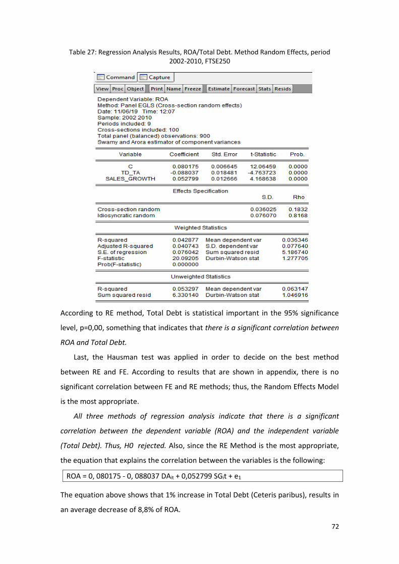
72
Table 27: Regression Analysis Results, ROA/Total Debt. Method Random Effects, period 2002-2010, FTSE250
According to RE method, Total Debt is statistical important in the 95% significance
level, p=0,00, something that indicates that there is a significant correlation between
ROA and Total Debt.
Last, the Hausman test was applied in order to decide on the best method
between RE and FE. According to results that are shown in appendix, there is no
significant correlation between FE and RE methods; thus, the Random Effects Model
is the most appropriate.
All three methods of regression analysis indicate that there is a significant
correlation between the dependent variable (ROA) and the independent variable
(Total Debt). Thus, H0 rejected. Also, since the RE Method is the most appropriate,
the equation that explains the correlation between the variables is the following:
ROA = 0, 080175 - 0, 088037 DAit + 0,052799 SGit + e1
The equation above shows that 1% increase in Total Debt (Ceteris paribus), results in
an average decrease of 8,8% of ROA.
73
As far as the first Model is concerned, the regression analysis results revealed
that there is a significant negative correlation between ROA and two of the three
independent variables (Long-term Debt and Total Debt), whereas there is a
significant positive correlation between ROA and Short-term Debt.
Model 2:
H0: There is no significant impact of Independent Variables on Return on Equity.
H1: There is a significant impact of Independent Variables on Return on Equity.
2.1 ROEit= β0 + β1SDAit+ β2SGit+e1
First, the method OLS is applied to estimate the regression function. The results are
shown in the appendix. Short-term Debt is not statistical important in the 95%
significance level, something that indicates that there is no significant correlation
between ROE and Short-term Debt, p=0,1428, or in other words, there is no
significant impact of Short-term Debt on ROA.
Next, the method Fixed Effects (FE) was applied to obtain better results since the
bias is minimized (the regression is realized for each data group separately). The
results are shown in the appendix. According to FE method, Short-term Debt is not
statistical important in the 95% significance level, p=0,7513, something that
indicates that there is no significant correlation between ROE and Short-term Debt.
Then, the Random Effects method is applied. The results of this method, and
specifically the coefficients, take into account the differences among the companies
as well as the differences among the years for a specific company. Thus, results show
the average impact of the independent variable (Short-term Debt) on the dependent
variable (ROE), when the independent variable changes one unit, through time and
among companies. Results are demonstrated on Table28, below.
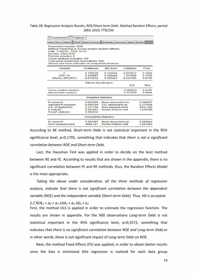
74
Table 28: Regression Analysis Results, ROE/Short-term Debt. Method Random Effects, period 2002-2010, FTSE250
According to RE method, Short-term Debt is not statistical important in the 95%
significance level, p=0,1705, something that indicates that there is not a significant
correlation between ROE and Short-term Debt.
Last, the Hausman Test was applied in order to decide on the best method
between RE and FE. According to results that are shown in the appendix, there is no
significant correlation between FE and RE methods; thus, the Random Effects Model
is the most appropriate.
Taking the above under consideration, all the three methods of regression
analysis, indicate that there is not significant correlation between the dependent
variable (ROE) and the independent variable (Short-term Debt). Thus, H0 is accepted.
2.2 ROEit = α0 + α1 LDAit + α2 SGit + e2 First, the method OLS is applied in order to estimate the regression function. The
results are shown in appendix. For the 900 observations Long-term Debt is not
statistical important in the 95% significance level, p=0,3572, something that
indicates that there is no significant correlation between ROE and Long-term Debt,or
in other words, there is not significant impact of Long-term Debt on ROE.
Next, the method Fixed Effects (FE) was applied, in order to obtain better results
since the bias is minimized (the regression is realized for each data group

75
separately). Results are shown in appendix. According to FE method, Long-term Debt
is not statistical important in the 95% significance level, p=0,2711, something that
indicates that there is not significant correlation between ROE and Long-term Debt.
Then, the Random Effects method is applied. The results of this method, and
specifically the coefficients, take into account the differences among the companies
as well as the differences among the years for a specific company. Thus, results show
the average impact of the independent variable (Long-term Debt) on the dependent
variable (ROE), when the independent variable changes one unit, through time and
among companies. The results are demonstrated in table29, below.
Table 29: Regression Analysis Results, ROE/Long-term Debt. Method Random Effects, period 2002-2010, FTSE250
According to RE method, Long-term Debt is not statistical important in the 95%
significance level, p=0,3503, something that indicates that there is not significant
correlation between ROE and Long-term Debt.
Last, the Hausman Test was applied in order to decide on the best method
between RE and FE. According to results that are shown in appendix, there is not
76
significant correlation between FE and RE methods; thus, the Random Effects Model
is the most appropriate.
Taking the above under consideration, all the three methods of regression
analysis, indicate that there is not significant correlation between the dependent
variable (ROE) and the independent variable (Long-term Debt). Thus, H0 is accepted.
2.3 ROEit = λ0 + λ1 DAit + λ2 SGit + e3
First, the method OLS is applied in order to estimate the regression function. Results
are shown in appendix. For the 900 observations Total Debt is not statistical
important in the 95% significance level, p=0,3776, something that indicates that
there is not significant correlation between ROE and Total Debt, or in other words,
there is not significant impact of Total Debt on ROE.
Next, the method Fixed Effects (FE) was applied, in order to obtain better results
since the bias is minimized (the regression is realized for each data group
separately). Results are shown in appendix. According to FE method, for the 900
observations, Total Debt is not statistical important in the 95% significance level,
p=0,6024, something that indicates that there is not significant correlation between
ROE and Total Debt.
Then, the Random Effects method was applied. The results of this method, and
specifically the coefficients, take into account the differences among the companies
as well as the differences among the years for a specific company. Thus, results show
the average impact of the independent variable (Total Debt) on the dependent
variable (ROE), when the independent variable changes one unit, through time and
among companies. Results are demonstrated on table30, below.
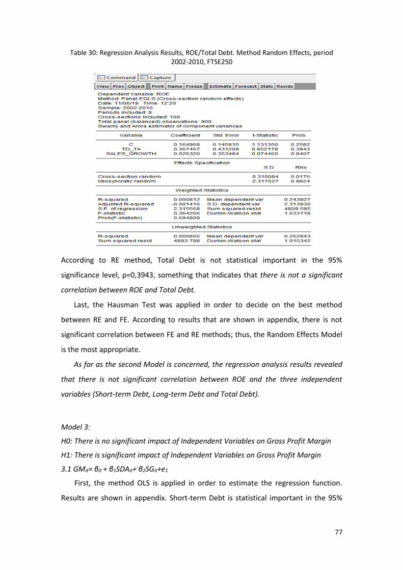
77
Table 30: Regression Analysis Results, ROE/Total Debt. Method Random Effects, period 2002-2010, FTSE250
According to RE method, Total Debt is not statistical important in the 95%
significance level, p=0,3943, something that indicates that there is not a significant
correlation between ROE and Total Debt.
Last, the Hausman Test was applied in order to decide on the best method
between RE and FE. According to results that are shown in appendix, there is not
significant correlation between FE and RE methods; thus, the Random Effects Model
is the most appropriate.
As far as the second Model is concerned, the regression analysis results revealed
that there is not significant correlation between ROE and the three independent
variables (Short-term Debt, Long-term Debt and Total Debt).
Model 3:
H0: There is no significant impact of Independent Variables on Gross Profit Margin
H1: There is significant impact of Independent Variables on Gross Profit Margin
3.1 GMit= β0 + β1SDAit+ β2SGit+e1
First, the method OLS is applied in order to estimate the regression function.
Results are shown in appendix. Short-term Debt is statistical important in the 95%

78
significance level, p=0,00, something that indicates that there is significant
correlation between Gross Profit Margin and Short-term Debt.
Next, the method Fixed Effects (FE) was applied, in order to obtain better results
since the bias is minimized (the regression is realized for each data group
separately). Results are shown in appendix. According to FE method, Short-term
Debt is not statistical important in the 95% significance level, p=0,5132, something
that indicates that there is not significant correlation between Gross Profit Margin
and Short-term Debt.
Table 31: Regression Analysis Results, Gross Profit Margin/Short-term Debt. Method Random Effects, period 2002-2010, FTSE250
Then, the Random Effects method is applied. According to RE method, Short-term
Debt is not statistical important in the 95% significance level, p=0,1704, something
that indicates that there is not significant correlation between Gross Profit Margin
and Short-term Debt.
Last, the Hausman Test was applied in order to decide on the best method
between RE and FE. According to results that are shown in appendix, there is
significant correlation between FE and RE methods; thus, the Fixed Effects Model is
the most appropriate.
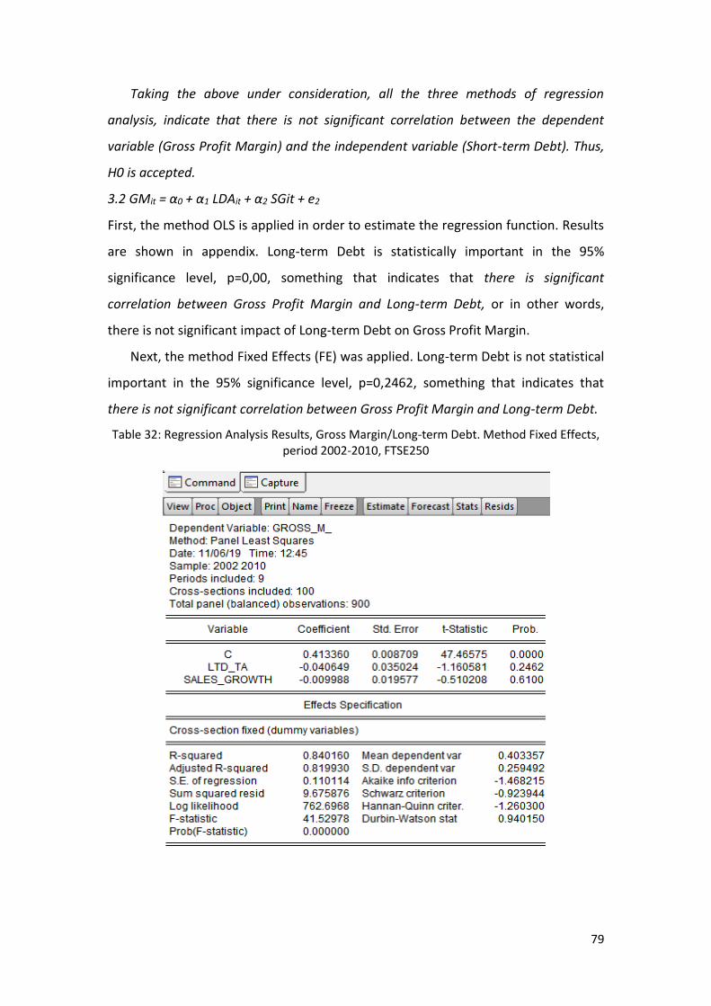
79
Taking the above under consideration, all the three methods of regression
analysis, indicate that there is not significant correlation between the dependent
variable (Gross Profit Margin) and the independent variable (Short-term Debt). Thus,
H0 is accepted.
3.2 GMit = α0 + α1 LDAit + α2 SGit + e2
First, the method OLS is applied in order to estimate the regression function. Results
are shown in appendix. Long-term Debt is statistically important in the 95%
significance level, p=0,00, something that indicates that there is significant
correlation between Gross Profit Margin and Long-term Debt, or in other words,
there is not significant impact of Long-term Debt on Gross Profit Margin.
Next, the method Fixed Effects (FE) was applied. Long-term Debt is not statistical
important in the 95% significance level, p=0,2462, something that indicates that
there is not significant correlation between Gross Profit Margin and Long-term Debt.
Table 32: Regression Analysis Results, Gross Margin/Long-term Debt. Method Fixed Effects, period 2002-2010, FTSE250
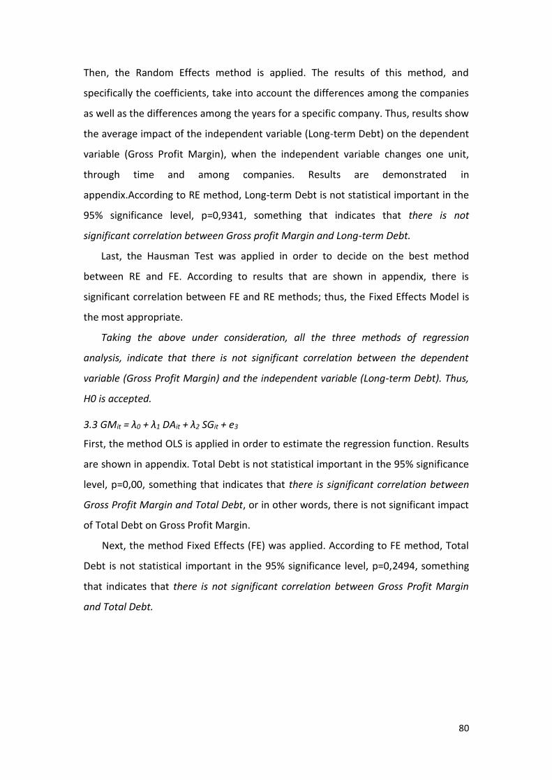
80
Then, the Random Effects method is applied. The results of this method, and
specifically the coefficients, take into account the differences among the companies
as well as the differences among the years for a specific company. Thus, results show
the average impact of the independent variable (Long-term Debt) on the dependent
variable (Gross Profit Margin), when the independent variable changes one unit,
through time and among companies. Results are demonstrated in
appendix.According to RE method, Long-term Debt is not statistical important in the
95% significance level, p=0,9341, something that indicates that there is not
significant correlation between Gross profit Margin and Long-term Debt.
Last, the Hausman Test was applied in order to decide on the best method
between RE and FE. According to results that are shown in appendix, there is
significant correlation between FE and RE methods; thus, the Fixed Effects Model is
the most appropriate.
Taking the above under consideration, all the three methods of regression
analysis, indicate that there is not significant correlation between the dependent
variable (Gross Profit Margin) and the independent variable (Long-term Debt). Thus,
H0 is accepted.
3.3 GMit = λ0 + λ1 DAit + λ2 SGit + e3
First, the method OLS is applied in order to estimate the regression function. Results
are shown in appendix. Total Debt is not statistical important in the 95% significance
level, p=0,00, something that indicates that there is significant correlation between
Gross Profit Margin and Total Debt, or in other words, there is not significant impact
of Total Debt on Gross Profit Margin.
Next, the method Fixed Effects (FE) was applied. According to FE method, Total
Debt is not statistical important in the 95% significance level, p=0,2494, something
that indicates that there is not significant correlation between Gross Profit Margin
and Total Debt.
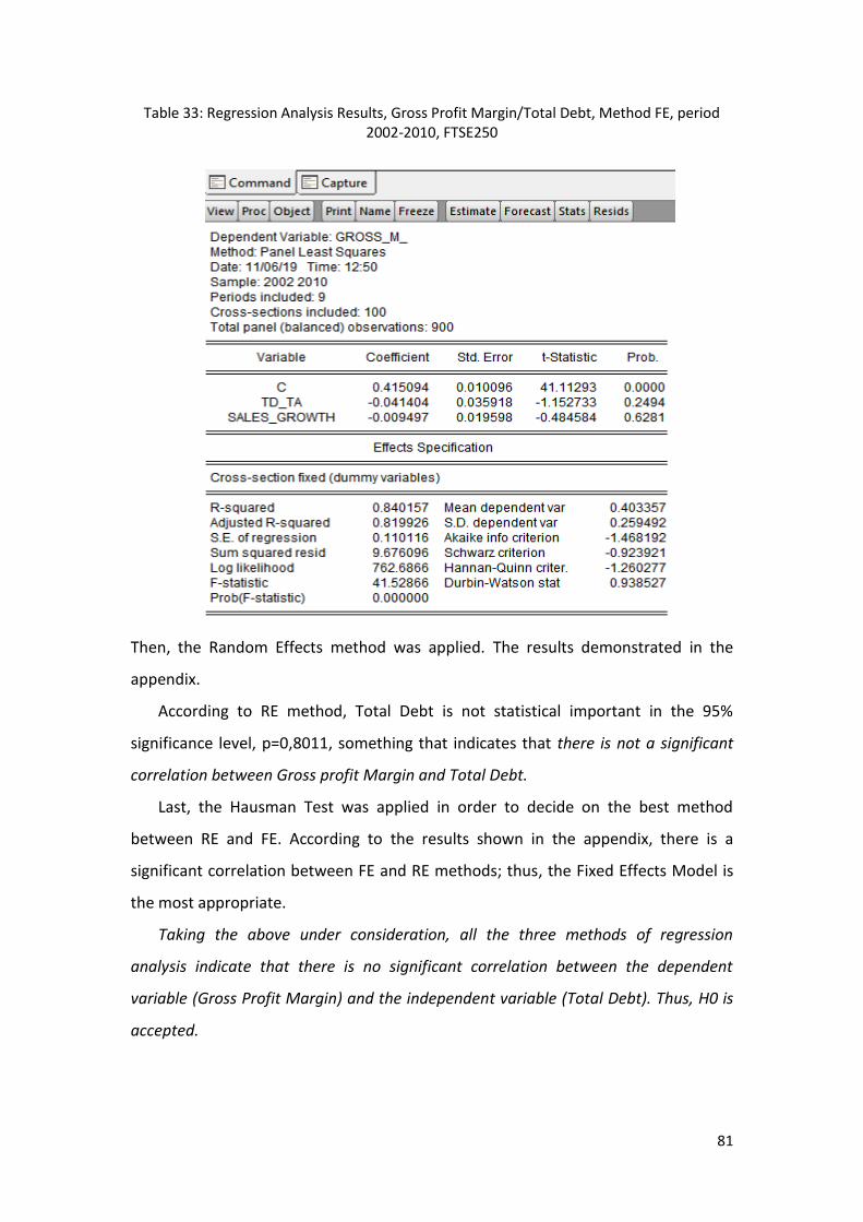
81
Table 33: Regression Analysis Results, Gross Profit Margin/Total Debt, Method FE, period 2002-2010, FTSE250
Then, the Random Effects method was applied. The results demonstrated in the
appendix.
According to RE method, Total Debt is not statistical important in the 95%
significance level, p=0,8011, something that indicates that there is not a significant
correlation between Gross profit Margin and Total Debt.
Last, the Hausman Test was applied in order to decide on the best method
between RE and FE. According to the results shown in the appendix, there is a
significant correlation between FE and RE methods; thus, the Fixed Effects Model is
the most appropriate.
Taking the above under consideration, all the three methods of regression
analysis indicate that there is no significant correlation between the dependent
variable (Gross Profit Margin) and the independent variable (Total Debt). Thus, H0 is
accepted.
82
6.4 FTSE 250 Period: 2011 – 2018
Results concerning the 100 companies of the FTSE250 Index for the years 2011-2018
are listed below.
First descriptive statistics for the variables were calculated and demonstrated in the
figure below:
Table 34: Descriptive statistics for FTSE250 data for the years 2011-2018
Table 34 demonstrates the descriptive statistics for the variables that used for all the
models, for the companies that belong to the FTSE250 Index, for the years 2011 –
2018. It seems that there is an important deviation among the ROE for the
companies of the sample.
Nevertheless, the average Gross Profit Margin, as well as ROE, is high. As far as
Short-term Debt and Long-term Debt are concerned, there is also a substantial
difference between the minimum and maximum values. 900 observations were
included.
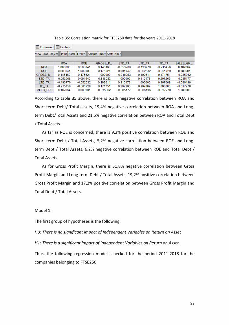
83
Table 35: Correlation matrix for FTSE250 data for the years 2011-2018
According to table 35 above, there is 5,3% negative correlation between ROA and
Short-term Debt/ Total assets, 19,4% negative correlation between ROA and Long-
term Debt/Total Assets and 21,5% negative correlation between ROA and Total Debt
/ Total Assets.
As far as ROE is concerned, there is 9,2% positive correlation between ROE and
Short-term Debt / Total Assets, 5,2% negative correlation between ROE and Long-
term Debt / Total Assets, 6,2% negative correlation between ROE and Total Debt /
Total Assets.
As for Gross Profit Margin, there is 31,8% negative correlation between Gross
Profit Margin and Long-term Debt / Total Assets, 19,2% positive correlation between
Gross Profit Margin and 17,2% positive correlation between Gross Profit Margin and
Total Debt / Total Assets.
Model 1:
The first group of hypotheses is the following:
H0: There is no significant impact of Independent Variables on Return on Asset
H1: There is a significant impact of Independent Variables on Return on Asset.
Thus, the following regression models checked for the period 2011-2018 for the
companies belonging to FTSE250:

84
1.3 ROAit= β0 + β1SDAit+ β2SGit+e1
First, the method OLS was applied. Results are included in appendix. Short-term Debt
is not statistically important in the 95% significance level, p=0,2776, something that
indicates that there is not significant correlation between ROA and Short-term Debt.
Next, the method Fixed Effects (FE) was applied, in order to obtain better results
since the bias is minimized (the regression is realized for each data group
separately). Results are included in the appendix. According to FE method, Short-
term Debt is statistically important in the 95% significance level, p=0,0458,
something that indicates that there is significant correlation between ROA and Short-
term Debt, or in other words, there is not significant impact of Short-term Debt on
ROA.
Then, the Random Effects method was applied. The results of this method, and
specifically the coefficients, take into account the differences among the companies
as well as the differences among the years for a specific company. Thus, results show
the average impact of the independent variable (Short-term Debt) on the dependent
variable (ROA), when the independent variable changes one unit, through time and
among companies. The results are shown in table 36, below.
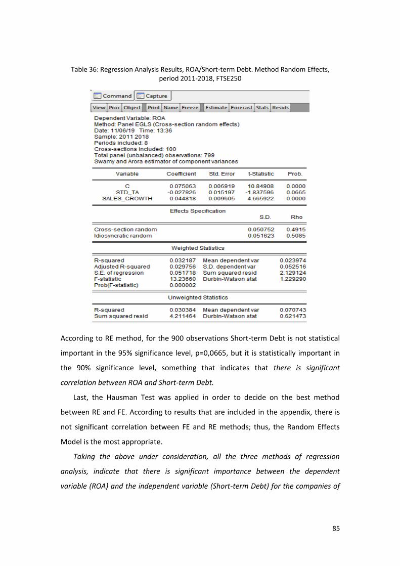
85
Table 36: Regression Analysis Results, ROA/Short-term Debt. Method Random Effects, period 2011-2018, FTSE250
According to RE method, for the 900 observations Short-term Debt is not statistical
important in the 95% significance level, p=0,0665, but it is statistically important in
the 90% significance level, something that indicates that there is significant
correlation between ROA and Short-term Debt.
Last, the Hausman Test was applied in order to decide on the best method
between RE and FE. According to results that are included in the appendix, there is
not significant correlation between FE and RE methods; thus, the Random Effects
Model is the most appropriate.
Taking the above under consideration, all the three methods of regression
analysis, indicate that there is significant importance between the dependent
variable (ROA) and the independent variable (Short-term Debt) for the companies of

86
FTSE250 and the period 2011-2018. Thus, H0 is rejected. The model developed is the
following:
ROAit= 0,075063- 0,027926 SDAit+ 0,044818 SGit+e1
The equation above shows that there is a positive correlation between the variables
and that 1% increase in Short-term Debt (Ceteris paribus) results in an average
decrease of 2,8% of ROA.
1.2. ROAit = α0 + α1 LDAit + α2 SGit + e2
First, the method OLS was applied to estimate the regression function. The results
are shown in appendix. Long-term Debt is statistical important in the 95%
significance level, p=0,00, something that indicates that there is a significant
correlation between ROA and Long-term Debt, or in other words, there is significant
impact of Long-term Debt on ROA.
Next, the method Fixed Effects (FE) applied to obtain better results since the bias
minimized (the regression is realized for each data group separately). According to
the FE method, Long-term Debt is statistical important in the 95% significance level,
p=0,1157, something that indicates that there is no significant correlation between
ROA and Long-term Debt.
Table 37: Regression Analysis Results, ROA/Long-term Debt, Method FE, period 2011-2018, FTSE250

87
Then, the Random Effects method is applied. The results of this method, and
specifically the coefficients, take into account the differences among the companies
as well as the differences among the years for a specific company. Thus, results show
the average impact of the independent variable (Long-term Debt) on the dependent
variable (ROA), when the independent variable changes one unit, through time and
among companies. The results demonstrated in the appendix. According to RE
method, Long-term Debt is statistical important in the 95% significance level,
p=0,0128, something that indicates that there is a significant correlation between
ROA and Long-term Debt.
Last, the Hausman Test applied in order to decide on the best method between
RE and FE. According to results that are shown in the appendix, there is a significant
correlation between FE and RE methods; thus, the Fixed Effects Model is the most
appropriate.
Taking the above under consideration, since the fixed effects method is the most
appropriate, there is no significant correlation between the dependent variable (ROA)
and the independent variable (Long-term Debt). Thus, H0 is accepted.
1.3 ROAit = λ0 + λ1 DAit + λ2 SGit + e3
First, the method OLS is applied to estimate the regression function. The results are
shown in the appendix. For the 900 observations, Total Debt is statistical important
in the 95% significance level, p=0,00, something that indicates that there is a
significant correlation between ROA and Total Debt, or in other words. There is a
significant impact of Total Debt on ROA. Also, there is a negative correlation
between the dependent and the independent variable.
Next, the method Fixed Effects (FE) applied, to obtain better results since the
bias minimized (the regression is realized for each data group separately). According
to FE method, Total Debt is not statistical important in the 95% significance level,
p=0,0844, but it is statistically important in the 90% significance level, something
that indicates that there is a significant correlation between ROA and Total Debt.

88
Table 38: Regression Analysis Results, ROA/Total Debt. Method Fixed Effects, period 2011-2018, FTSE250
Then, the Random Effects method is applied. According to the RE method, Total
Debt is statistical important in the 95% significance level, p=0,00, something that
indicates that there is a significant correlation between ROA and Total Debt.
Last, the Hausman Test was applied to decide on the best method between RE
and FE. According to results that are shown in the appendix, there is a significant
correlation between FE and RE methods; thus, the Fixed Effects Model is the most
appropriate.
All three methods of regression analysis indicate that there is a significant
correlation between the dependent variable (ROA) and the independent variable
(Total Debt). Thus, H0 rejected. Also, since the FE Method is the most appropriate,
the equation that explains the correlation between the variables is the following:
ROA = 0, 070633 - 0, 013573 DAit + 0,042332 SGit + e1
The equation above shows that 1% increase in Total Debt (Ceteris paribus),
results to an average decrease of 1,36% of ROA.

89
As far as the first Model is concerned, the regression analysis results revealed
that there is significant negative correlation between ROA and two of the three
independent variables (Short-term Debt and Total Debt).
Model 2:
H0: There is no significant impact of Independent Variables on Return on Equity.
H1: There is a significant impact of Independent Variables on Return on Equity.
2.1 ROEit= β0 + β1SDAit+ β2SGit+e1
First, the method OLS is applied to estimate the regression function. The results are
shown in the appendix. Short-term Debt is not statistical important in the 95%
significance level, something that indicates that there is a significant correlation
between ROE and Short-term Debt, p=0,00, or in other words, there is a significant
impact of Short-term Debt on ROA.
Next, the method Fixed Effects (FE) was applied, to obtain better results since
the bias is minimized (the regression is realized for each data group separately). The
results are shown in appendix. According to FE method, Short-term Debt is not
statistical important in the 95% significance level, p=0,4228, something that
indicates that there is not a significant correlation between ROE and Short-term
Debt.
Then, the Random Effects method is applied. The results of this method, and
specifically the coefficients, take into account the differences among the companies
as well as the differences among the years for a specific company. Thus, results show
the average impact of the independent variable (Short-term Debt) on the dependent
variable (ROE), when the independent variable changes one unit, through time and
among companies. The results are demonstrated in table39, below.
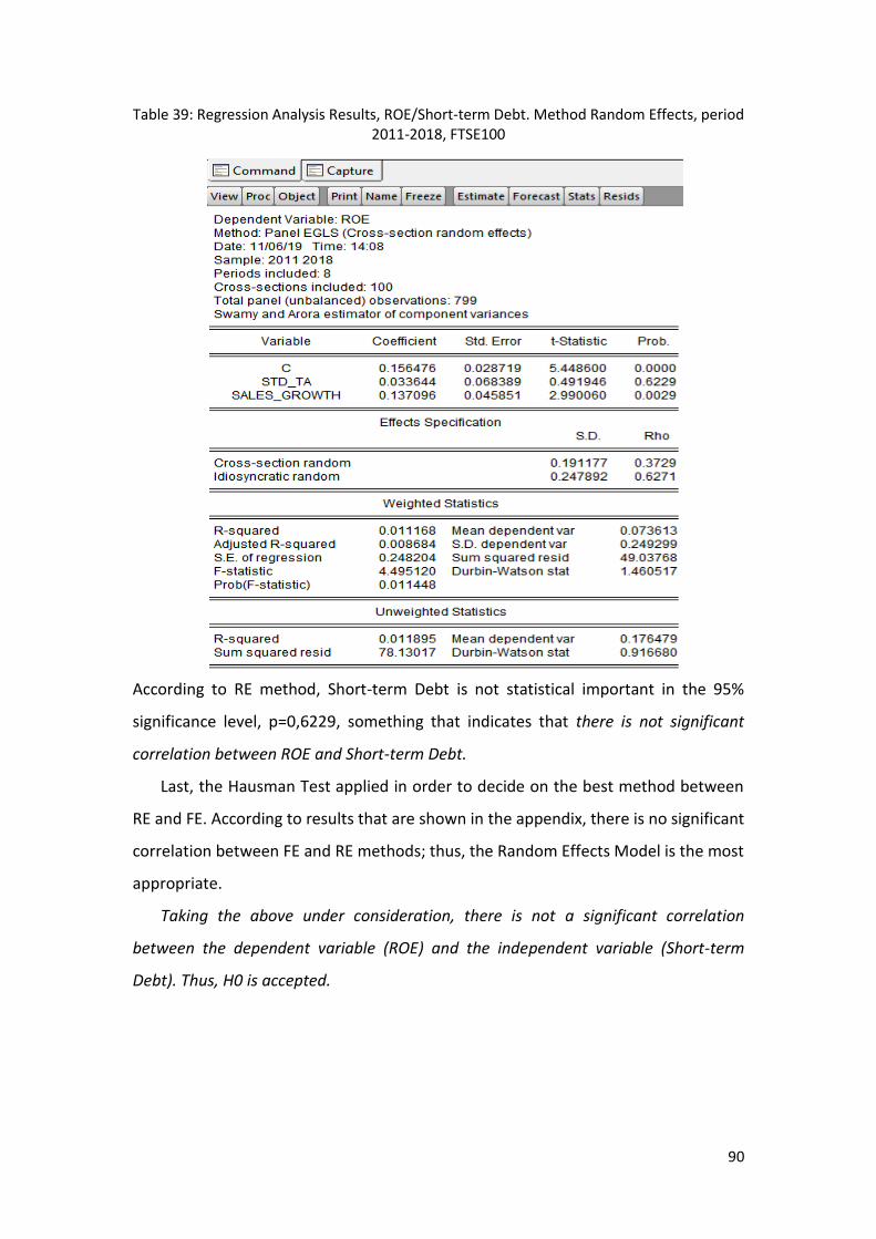
90
Table 39: Regression Analysis Results, ROE/Short-term Debt. Method Random Effects, period 2011-2018, FTSE100
According to RE method, Short-term Debt is not statistical important in the 95%
significance level, p=0,6229, something that indicates that there is not significant
correlation between ROE and Short-term Debt.
Last, the Hausman Test applied in order to decide on the best method between
RE and FE. According to results that are shown in the appendix, there is no significant
correlation between FE and RE methods; thus, the Random Effects Model is the most
appropriate.
Taking the above under consideration, there is not a significant correlation
between the dependent variable (ROE) and the independent variable (Short-term
Debt). Thus, H0 is accepted.
91
2.2 ROEit = α0 + α1 LDAit + α2 SGit + e2
First, the method OLS is applied in order to estimate the regression function. The
results are shown in the appendix. Long-term Debt is not statistical important in the
95% significance level, p=0,5068, something that indicates that there is no significant
correlation between ROE and Long-term Debt, or in other words; there is not the
significant impact of Long-term Debt on ROE.
Next, the method Fixed Effects (FE) was applied, to obtain better results since
the bias is minimized (the regression is realized for each data group separately). The
results are shown in the appendix. According to FE method, Long-term Debt is not
statistical important in the 95% significance level, p=0,6846, something that
indicates that there is not a significant correlation between ROE and Long-term Debt.
Then, the Random Effects method is applied. The results of this method, and
specifically the coefficients, take into account the differences among the companies
as well as the differences among the years for a specific company. Thus, results show
the average impact of the independent variable (Long-term Debt) on the dependent
variable (ROE), when the independent variable changes one unit, through time and
among companies. The results are demonstrated in table 40, below.

92
Table 40: Regression Analysis Results, ROE/Long-term Debt. Method Random Effects, period 2011-2018, FTSE250
According to the RE method, Long-term Debt is not statistical important in the 95%
significance level, p=0,5068, something that indicates that there is no significant
correlation between ROE and Long-term Debt.
Last, the Hausman Test was applied in order to decide on the best method
between RE and FE. According to results that are shown in the appendix, there is no
significant correlation between FE and RE methods; thus, the Random Effects Model
is the most appropriate.
Taking the above under consideration, all the three methods of regression
analysis, indicate that there is no significant correlation between the dependent
variable (ROE) and the independent variable (Long-term Debt). Thus, H0 is accepted.
2.3 ROEit = λ0 + λ1 DAit + λ2 SGit + e3
First, the method OLS is applied in order to estimate the regression function. The
results are shown in the appendix. Total Debt is not statistical important in the 95%
significance level, p=0,1307, something that indicates that there is no significant
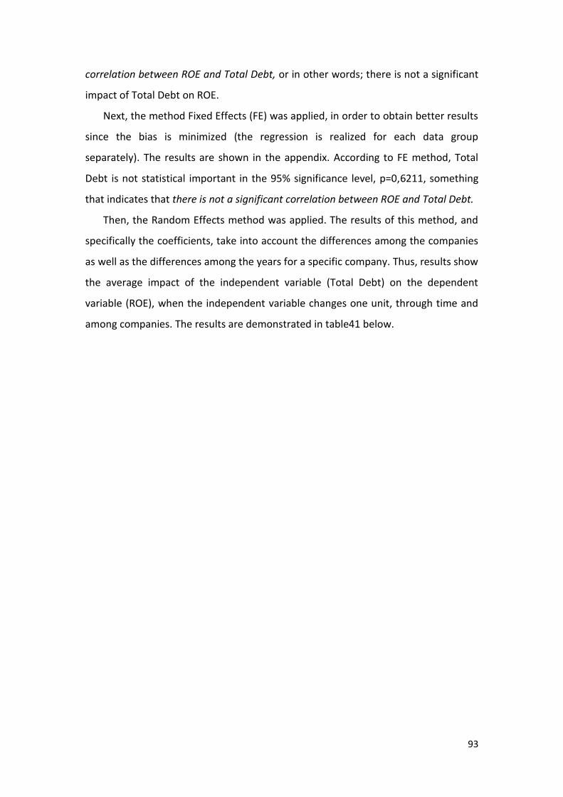
93
correlation between ROE and Total Debt, or in other words; there is not a significant
impact of Total Debt on ROE.
Next, the method Fixed Effects (FE) was applied, in order to obtain better results
since the bias is minimized (the regression is realized for each data group
separately). The results are shown in the appendix. According to FE method, Total
Debt is not statistical important in the 95% significance level, p=0,6211, something
that indicates that there is not a significant correlation between ROE and Total Debt.
Then, the Random Effects method was applied. The results of this method, and
specifically the coefficients, take into account the differences among the companies
as well as the differences among the years for a specific company. Thus, results show
the average impact of the independent variable (Total Debt) on the dependent
variable (ROE), when the independent variable changes one unit, through time and
among companies. The results are demonstrated in table41 below.
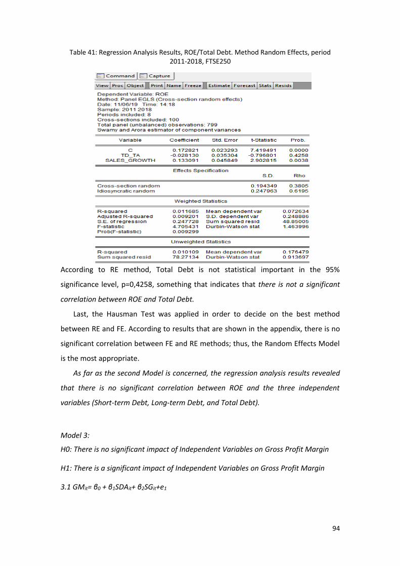
94
Table 41: Regression Analysis Results, ROE/Total Debt. Method Random Effects, period 2011-2018, FTSE250
According to RE method, Total Debt is not statistical important in the 95%
significance level, p=0,4258, something that indicates that there is not a significant
correlation between ROE and Total Debt.
Last, the Hausman Test was applied in order to decide on the best method
between RE and FE. According to results that are shown in the appendix, there is no
significant correlation between FE and RE methods; thus, the Random Effects Model
is the most appropriate.
As far as the second Model is concerned, the regression analysis results revealed
that there is no significant correlation between ROE and the three independent
variables (Short-term Debt, Long-term Debt, and Total Debt).
Model 3:
H0: There is no significant impact of Independent Variables on Gross Profit Margin
H1: There is a significant impact of Independent Variables on Gross Profit Margin
3.1 GMit= β0 + β1SDAit+ β2SGit+e1
95
First, the method OLS is applied to estimate the regression function. The results
are shown in the appendix. Short-term Debt is statistical important in the 95%
significance level, p=0,00, something that indicates that there is a significant
correlation between Gross Profit Margin and Short-term Debt.
Next, the method Fixed Effects (FE) applied, to obtain better results since the
bias is minimized (the regression is realized for each data group separately). The
results are shown in the appendix. According to FE method, Short-term Debt is not
statistical important in the 95% significance level, p=0,00, something that indicates
that there is a significant correlation between Gross Profit Margin and Short-term
Debt.
Table 42: Regression Analysis Results, Gross Profit Margin/Short-term Debt. Method Fixed Effects, period 2011-2018, FTSE250
Then, the Random Effects method is applied. According to RE method, Short-term
Debt is not statistical important in the 95% significance level, p=0,00, something that
indicates that there is no significant correlation between Gross Profit Margin and
Short-term Debt.
96
Last, the Hausman Test applied in order to decide on the best method between
RE and FE. According to results that are shown in the appendix, there is a significant
correlation between FE and RE methods; thus, the Fixed Effects Model is the most
appropriate.
Taking the above under consideration, all the three methods of regression
analysis, indicate that there is a significant correlation between the dependent
variable (Gross Profit Margin) and the independent variable (Short-term Debt). Thus,
H0 is rejected. Since the FE model is most appropriate, the equation is the following:
GMit= 0,461014 – 0,092912 SDAit- 0,024465 SGit+e1
3.2 GMit = α0 + α1 LDAit + α2 SGit + e2
First, the method OLS is applied to estimate the regression function. The results are
shown in the appendix. Long-term Debt is statistically important in the 95%
significance level, p=0,00, something that indicates that there is a significant
correlation between Gross Profit Margin and Long-term Debt, or in other words,
there is not the significant impact of Long-term Debt on Gross Profit Margin.
Next, the method Fixed Effects (FE) was applied. Long-term Debt is not statistical
important in the 95% significance level, p=0,3168, something that indicates that
there is not a significant correlation between Gross Profit Margin and Long-term
Debt.
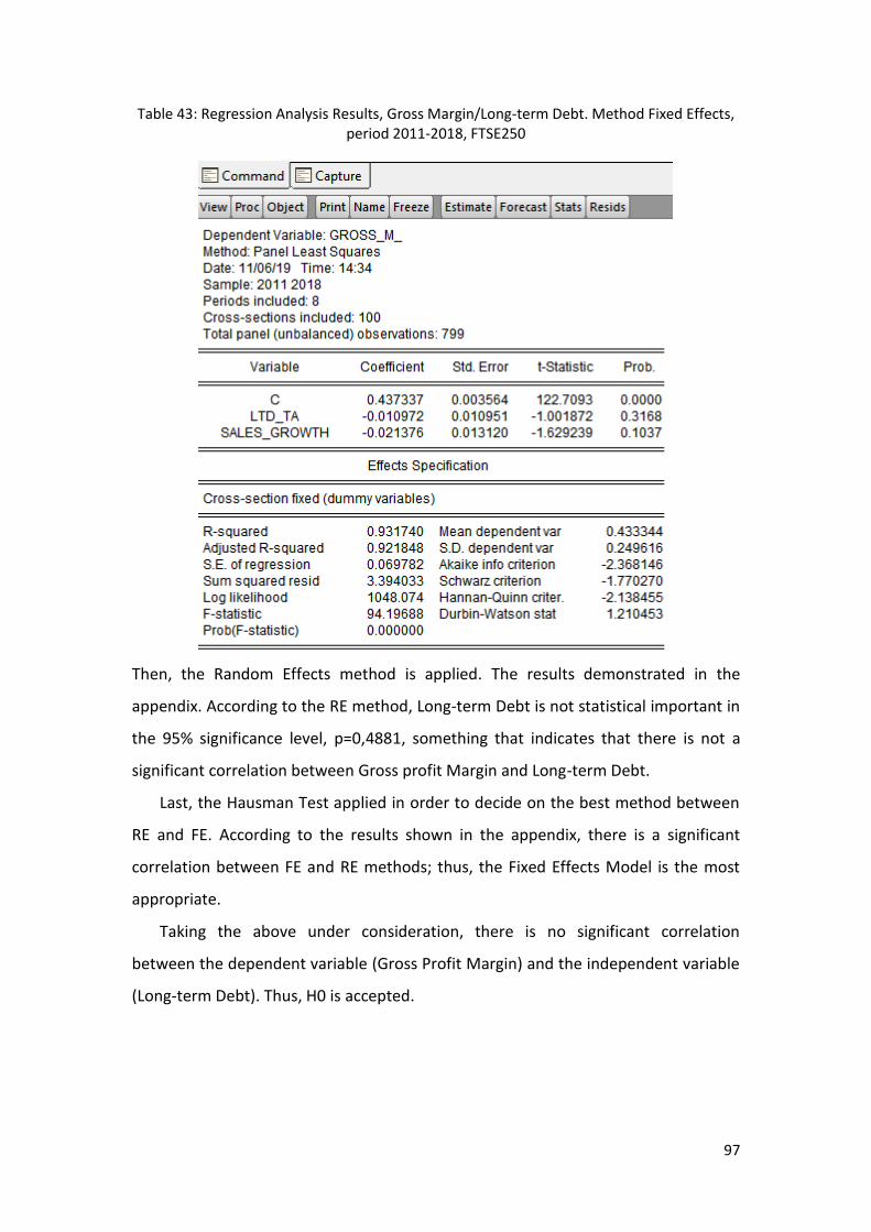
97
Table 43: Regression Analysis Results, Gross Margin/Long-term Debt. Method Fixed Effects, period 2011-2018, FTSE250
Then, the Random Effects method is applied. The results demonstrated in the
appendix. According to the RE method, Long-term Debt is not statistical important in
the 95% significance level, p=0,4881, something that indicates that there is not a
significant correlation between Gross profit Margin and Long-term Debt.
Last, the Hausman Test applied in order to decide on the best method between
RE and FE. According to the results shown in the appendix, there is a significant
correlation between FE and RE methods; thus, the Fixed Effects Model is the most
appropriate.
Taking the above under consideration, there is no significant correlation
between the dependent variable (Gross Profit Margin) and the independent variable
(Long-term Debt). Thus, H0 is accepted.

98
3.3 GMit = λ0 + λ1 DAit + λ2 SGit + e3
First, the method OLS is applied to estimate the regression function. The results are
shown in the appendix. Total Debt is not statistical important in the 95% significance
level, p=0,00, something that indicates that there is a significant correlation between
Gross Profit Margin and Total Debt, or in other words, there is no significant impact
of Total Debt on Gross Profit Margin.
Next, the method Fixed Effects (FE) was applied. According to the FE method,
Total Debt is not statistical important in the 95% significance level, p=0,17,
something that indicates that there is no significant correlation between Gross Profit
Margin and Total Debt.
Table 44: Regression Analysis Results, Gross Profit Margin/Total Debt, Method FE, period 2011-2018, FTSE250
Then, the Random Effects method was applied. The results are demonstrated in the
appendix.
According to the RE method, Total Debt is not statistical important in the 95%
significance level, p=0,2728, something that indicates that there is no significant
correlation between Gross profit Margin and Total Debt.

99
Last, the Hausman test was applied to decide on the best method between RE
and FE. According to the results shown in the appendix, there is a significant
correlation between FE and RE methods; thus, the Fixed Effects Model is the most
appropriate.
Taking the above under consideration, there is not a significant correlation
between the dependent variable (Gross Profit Margin) and the independent variable
(Total Debt). Thus, H0 is accepted.

100
6.Conclusions
6.1 Key Results
For the period 2002 – 2010, for the FTSE100 companies:
o In respect of the first model is concerned, long term debt and Total
Debt have significant, negative impact on ROA, whereas there is no
significant impact of short-term debt on ROA. Thus, H0 is partly
accepted.
o As far as the second Model is concerned, the regression analysis
results revealed that there is no significant correlation between ROE
and the three independent variables (Short-term Debt, Long-term
Debt and Total Debt). Thus, H0 is accepted.
o There is not a significant correlation between the dependent variable
(Gross Profit Margin) and the independent variables. Thus, H0 is
accepted
For the period 2010 – 2018, for the FTSE100 companies:
o Concerning the first model, all the three methods of regression
analysis indicate that there is not significant importance between the
dependent variable (ROA) and the independent variables. Thus, H0 is
accepted.
o Towards the second model concerned, there is a significant
correlation between ROE and the three independent variables (Short-
term Debt, Long-term Debt and Total Debt), at the 95% and the 90%
significance level. These results are under other researchers' findings
(Gill et al., 2011).
o As far as the third Model is concerned, the regression analysis results
revealed that there is no significant correlation between Gross Profit
Margin and the two independent variables (Long-term Debt and Total
Debt). There is a significant correlation between Short-term Debt and
Gross Profit Margin.

101
For the period 2002-2010, for FTSE250 companies:
o Because of the first Model, the regression analysis results revealed
that there is a significant negative correlation between ROA and two
of the three independent variables (Long-term Debt and Total Debt),
whereas there is a significant positive correlation between ROA and
Short-term Debt. These results are in consistence with other
researchers’ results (Chen & Chen, 2011; Tailab, 2015; Vaicondam &
Ramakrishnan, 2017).
o As far as the second Model is concerned, the regression analysis
results revealed that there is not a significant correlation between
ROE and the three independent variables (Short-term Debt, Long-
term Debt and Total Debt).
o For the third model, all three methods of regression analysis indicate
that there is not a significant correlation between the dependent
variable (Gross Profit Margin) and the independent variables. Thus,
H0 is accepted.
For the period 2011-2018, for FTSE250 companies:
o As far as the first Model is concerned, the regression analysis results
revealed that there is a significant negative correlation between ROA
and two of the three independent variables (Short-term Debt and
Total Debt).
o As far as the second Model is concerned, the regression analysis
results revealed that there is no significant correlation between ROE
and the three independent variables (Short-term Debt, Long-term
Debt and Total Debt).
o All the three methods of regression analysis indicate that there is a
significant correlation between the dependent variable (Gross Profit
Margin) and the independent variable (Short-term Debt), whereas
there is not significant correlation between Gross Profit Margin and
the other two independent variables. Previous research has revealed
an only positive correlation between gross profit margin and long-
term debt (Voulgaris, 2002).

102
These results reveal that profitable firms do not rely on debt to finance their
operations. The fact that ROA is the ratio that is correlated with profitability, maybe
since most of the companies in the sample belong to the industrial sector. On the
other hand, the positive correlation between profitability and short – term debt is
since companies, in the short term, want to borrow from banks because of the
benefits they receive since interest tax is deductible (Sibindi, 2016).
The correlation, even if it exists, it is not always important in terms of percentage.
The important correlation applies to the following cases:
i. Short term debt (62,4%), Long-term debt (88,2%), and Total debt
(79,5%) to ROE, for the period 2011-2018 for the companies of the
FTSE100 Index, something that shows that debt structure choice for
firms can alter their operating profit significantly.
ii. Short –term debt (19,3% & 38,2%) to Gross Profit Margin for the
period 2011-2018 for the companies of the FTSE100 and the FTSE250
Index respectively, something that shows that the capital structure
choice for these firms can alter their operating profit.
Also, as far as the two different periods of investigation are concerned, for
FTSE100 Index companies, results are almost the same, i.e., only ROA is correlated
with firms Capital Structure. The difference is that short-term debt is not significantly
correlated with ROA for the years before the crisis, whereas it positively correlated
with ROA during the years of crisis. This may be since during crisis, firms needed to
borrow to increase their profitability, since revenues decreased. For the FTSE250
Index, during the years of crisis, only one dependent variable, Gross Profit Margin, is
negatively correlated with one of the independent variables, Short-term debt. For
the years before the crisis, ROA correlated with long-term debt and total debt. These
results indicate that the effect of capital structure on profitability changed during the
years of crisis.
Last, between the two periods, descriptive statics reveal that all dependent
variables changed. It is indicative that the companies of the FTSE100 Index were
more affected than the companies of the FTSE250 Index.
Generally, the results indicate that capital structure affects profitability, to a
greater or lower extent. There is not a specific rule for firms to follow since the

103
capital structure is also an internal decision and can be affected by several factors.
Nevertheless, the present study adds in the existing literature by confirming previous
research results as well as by revealing new relationships between the variables
selected for the research.
6.2 Further Research
Eventually, wider research on this topic could be done by adding more independent
variables and presenting Total Assets instead of Total Debt. It would still be possible
to add additional control variables to be more stable in our sample. Moreover, the
balanced participation of all sectors in the research it would be an extra clue about
the needs of each business area separately.

104
Bibliography
1. Abeywardhana, D.K.Y. (2015). Capital Structure and Profitability: An Empirical Analysis of SMEs in the UK, Journal of Emerging Issues in Economics, Finance and Banking, 4(2), 1-14
2. Abor, J., (2005). “The effect of capital structure on profitability: empirical analysis of listed firms in Ghana”. Journal of Risk Finance, 6(5), pp. 438-45.
3. Addae, A.A., Baasi, M.N. & Hughes, D. (2013). The Effects of Capital Structure on Profitability of Listed Firms in Ghana, European Journal of Business and Management, 5 (31), 215-229
4. Ahmad, T. (2014). Impact of Capital Structure on Profitability: An Empirical Analysis of Cement Sector of Pakistan, Research Journal of Finance and Accounting, 5(17), 49-54
5. Ahmed, N., Ahmed, Z. & Ahmed, I. (2010). Determinants of Capital Structure: A Case of Life Insurance Sector of Pakistan. European Journal of Economics, Finance and Administrative Sciences, 24, 7-12
6. Al Kahtani, N. and Al Eraij, M. (2018). Does capital structure matter? Reflection on capital structure irrelevance theory: Modigliani-Miller theorem (MM 1958). International Journal of Financial Services Management, 9(1), p.39.
7. Antoniou, A., Guney, Y. & Paudyal, K. (2008). The Determinants of Capital Structure: Capital Market Oriented Versus Bank-Oriented Institutions, Journal of Financial and Quantitative Analysis, 43(01), 59-92
8. Baker, M., Wurgler, J., (2002), ‘Market Timing and Capital Structure’, The Journal of Finance, 57, pp.1-32.
9. Baltagi, B., 2008. Econometric analysis of panel data. John Wiley & Sons.
10. Barclay, M.J. & Smith, C.W. (2005). The Capital Structure Puzzle: The Evidence Revisited, Journal of Applied Corporate Finance, 17(1), 8-17
11. Bennett, M., Donnelly, R., (1993), ‘The Determinants of Capital Structure: Some UK Evidence’, The British Accounting Review, 25, pp. 43-59.
12. Bolton, Patrick, and David S Scharfstein, 1996, Optimal debt structure and the number of creditors, Journal of Political Economy, pp.1–25.
13. Chen, L.J. & Chen, S.Y. (2011). The influence of profitability on firm value with capital structure as the mediator and firm size and industry as moderators, Investment Management and Financial Innovations, 8(3), 121-129
14. Chisti, K.A., Ali, K. & Sangmi, M.D. (2013). Impact of capital structure on profitability of listed companies (evidence from India), The USV Annals of Economics and Public Administration, 13(1), 183-191
15. Chou, S. R., Yang, J. A. and Lee, C. H. (2011) Determinants of capital structure in Taiwan 50: a structure equation modeling approach, Sun Yat-Sen Management Review, 19, pp. 225–77.
16. Claver, E., Molina, J., & Tari, J. (2002). Firm and industry effects on firm profitability: a Spanish empirical analysis. European Management Journal, 20(3). pp. 321-328.

105
17. de Mesquita, J.M.C. & Lara, J.E. (2015). Capital Structure and Profitability: The Brazilian Case, [online] available at: https://www.researchgate.net/publication/265235369_CAPITAL_STRUCTURE_AND_PROFITABILITY_THE_BRAZILIAN_CASE, accessed: November 10, 2019
18. Deesomsak, R., Paudyal, K., Pescetto, G., (2004), ‘The Determinants of Capital Structure: Evidence from the Asia Pacific Region’, Journal of Multinational Financial Management, 14, pp. 387-405.
19. Eriotis, N. P., Frangouli, Z., & Ventoura-Neokosmides, Z. (2011). Profit margin and capital structure: An empirical relationship. The Journal of Applied Business Research, 18(2), pp. 85-88.
20. Fama, E. F., French, K. R., (2002), ‘Testing Trade‐Off and Pecking Order Predictions about Dividends and Debt’, Review of Financial Studies, 15, pp. 1-33.
21. Frank, M.Z. & Goyal, V.K. (2009), Capital Structure Decisions: Which Factors Are Reliably Important? Financial Management, 38(1), 1-37
22. Friend, I., & Lang, L. H. P. (1988). An empirical test of the impact of managerial self-interest on corporate capital structure. Journal of Finance, 43, pp. 271– 281.
23. Gill, A., Biger, N. & Mathur, N. (2011). The Effect of Capital Structure on Profitability: Evidence from the United States, International Journal of Management, 28(4), 3-15
24. Hamid, M.A., Abdullah, A. & Kamaruzzaman, N.A. (2015). Capital Structure and Profitability in Family and Non-Family Firms: Malaysian evidence, Procedia Economics and Finance, 31, 44-55
25. Harris, M. & Raviv, A. (1991). The Theory of Capital Structure, The Journal of Finance, 46(1), 297-355
26. Jong, A., Kabir, R., Nguyen, T. T., (2008), ‘Capital structure around the world: The roles of firm- and country-specific determinants’, Journal of Banking & Finance, Volume 32, Issue 9, September 2008, pp. 1954-1969.
27. Keith, G. (1998). Determinants of growth and profitability in small entrepreneurial firms. International Journal of Entrepreneurial Behavior & Research, 4(1), pp. 18-27
28. Leary, M. T., Roberts, M. R., (2005), ‘Do Firms Rebalance Their Capital Structures?’
29. Mashavave, F. & Tsaurai, K. (2015). Capital Structure and Porfitability, A case of JSE Listed Companies, Risk governance & control: financial markets & institutions, 5(1), 81-93
30. Modigliani, F., Miller, M. H., (1958), ‘The cost of capital, corporation finance and the theory of investment’, The American Economic Review, 261-297.
31. Modigliani, F., Miller, M. H., (1963), ‘Corporate income taxes and the cost of capital: A correction’, The American Economic Review, 53, 433-443.
32. Myers, S. C., (1984), ‘The capital structure puzzle’, The Journal of Finance, 39, pp. 575-592.
33. Myers, S.C. (2001). Capital Structure, The Journal of Economic Perspectives, 15(2), 81-102
106
34. Nasimi, A.N. (2016). Effect of Capital Structure on Firm Profitability (An Empirical Evidence from London, UK), Global Journal of management and Business research: C Finance, 16(4), 9-19
35. Nishanthini, A. and Nimalathasan, B. (2014). Determinants of profitability: a case study of listed manufacturing companies in Sri Lanka. Journal of Management, 8(1), p.42.
36. Oino, I. & Ukaegbu, B. (2015). The impact of profitability on capital structure and speed of adjustment: An empirical examination of selected firms in Nigerian Stock Exchange, Research in International Business and Finance, 35, 111-121
37. Oino, I. and Ukaegbu, B. (2015). The impact of profitability on capital structure and speed of adjustment: An empirical examination of selected firms in Nigerian Stock Exchange. Research in International Business and Finance, 35, pp.111-121.
38. Ozkan, A., (2001), ‘Determinants of Capital Structure and Adjustment to Long Run Target: Evidence from UK Company Panel Data’, Journal of Business Finance & Accounting, 28, pp.175-198.
39. Pasiouras, F. & Kosmidou, K. (2007). Factors influencing the profitability of domestic and foreign commercial banks in the European Union, Research in International Business and Finance, 21, 222-237
40. Petria, N., Capraru, B. & Ihnatov, J. (2015). Determinants of banks’ profitability: evidence from EU 27 banking systems, Procedia Economics and Finance, 20, 518-524
41. Rasiah, D. & Kim, P.K. (2011). A Theoretical Review on The Use of The Static Trade Off Theory, The Pecking Order Theory and The Agency Cost Theory of Capital Structure, International Research Journal of Finance and Economics, 63, 150-159
42. Scott, J. H., (1976), ‘A theory of optimal capital structure’, The Bell Journal of Economics, 7, pp.33-54.
43. Sharma, A. and Kumar, S. (2010). Effect of Working Capital Management on Firm Profitability. Global Business Review, 12(1), pp.159-173.
44. Shubita, M.F. & Maroof, J.A. (2012). The Relationship between Capital Structure and Profitability, International Journal of Business and Social Science, 3(16), 104-112
45. Sibindi, A.B. (2016). Determinants of Capital Structure: A Literature Review, Risk Governance & Control: Financial Markets & Institutions, 6(4), 227-238
46. Singh, N.P. & Bagga, M. (2019). The Effect of Capital Structure on Profitability: An Empirical Panel Data Study, Jindal Journal of Business Research, 1–13
47. Soultan, A.S. & Adam, M.H.M. (2015). The effect of Capital Structure on Profitability: An empirical Analysis of Listed Firms in Iraq, European Journal of Accounting, Auditing and Finance Research, 3(2), 61-78
48. Stekla, J. & Grycova, M. (2015). The Relationship between Capital Structure and profitability of the Limited Liability Companies, Acta universiatis Bohemiae Meridionalis, 18(2), 32-41
49. Tailab, M.M.K. (2014). he Effect of Capital Structure on Profitability of Energy American Firms, International Journal of Business and Management Invention, 3(12),
54-61The Journal of Finance, 60, pp. 2575-2619.
50. Titman, S. & Wessels, R. (1988). The determinants of Capital Structure Choice, The journal of finance, 43(1), 1-19

107
51. Vaicondam, Y. & Ramakrishnan, S. (2017). Capital Structure and Profitability Across Malaysian Listed Firms, Advanced Science Letters, 23, 9275-9278
52. Voulgaris, F., Asteriou, D. & Agiomirgianakis, G. (2002). Capital structure, asset utilization, profitability and growth in the Greek manufacturing sector, Applied Economics, 34(11), 1379-1388
53. Williams, R., 2015. Panel data 4: Fixed effects vs random effects models. University of Notre Dame
54. Zaid, N. A. M., Ibrahim, W. M. F. W., & Zulqernain, N. S. (2014). The Determinants of profitability: Evidence from Malaysian construction companies. Proceedings of 5th Asia-Pacific Business Research Conference. Kuala Lumpur, Malaysia
55. Information about Indexes are taken from London Stock Exchange: https://www.londonstockexchange.com/home/homepage.htm
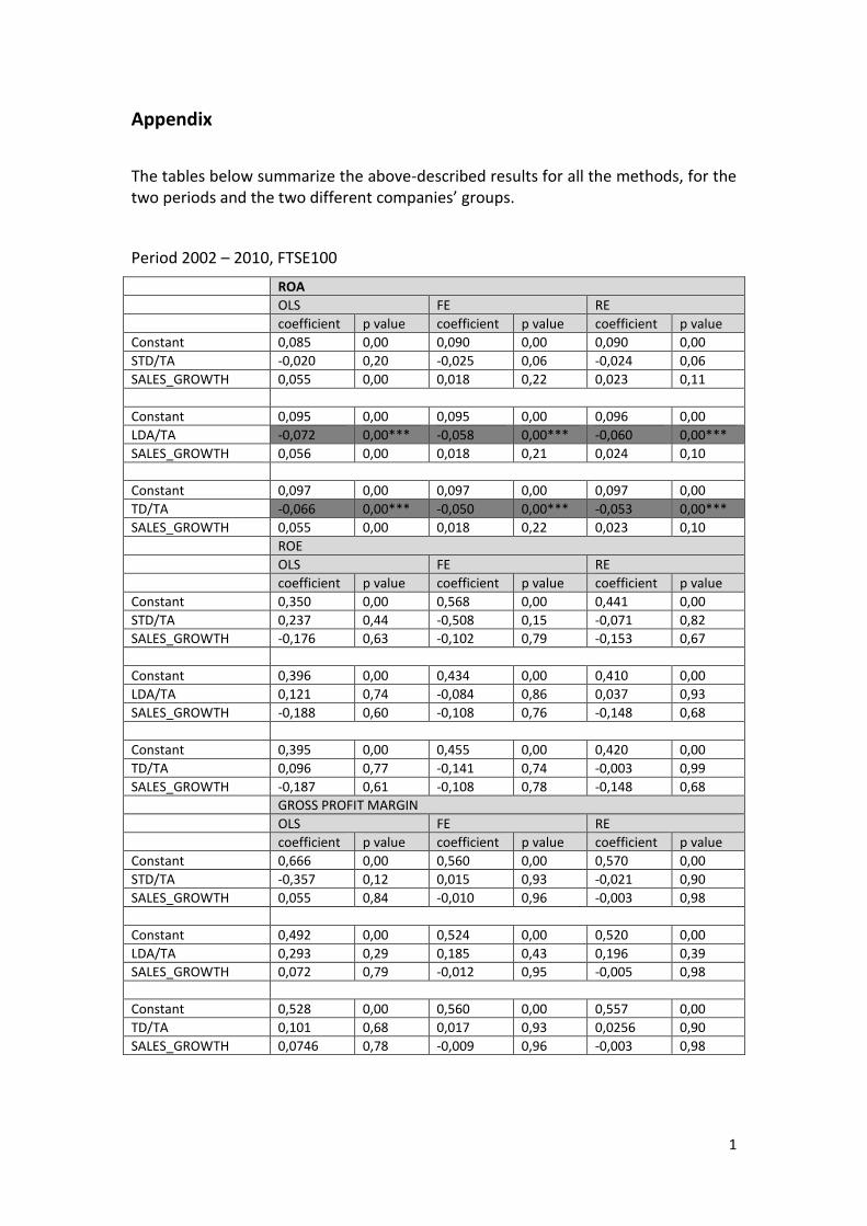
1
Appendix
The tables below summarize the above-described results for all the methods, for the two periods and the two different companies’ groups.
Period 2002 – 2010, FTSE100
ROA
OLS FE RE
coefficient p value coefficient p value coefficient p value
Constant 0,085 0,00 0,090 0,00 0,090 0,00
STD/TA -0,020 0,20 -0,025 0,06 -0,024 0,06
SALES_GROWTH 0,055 0,00 0,018 0,22 0,023 0,11
Constant 0,095 0,00 0,095 0,00 0,096 0,00
LDA/TA -0,072 0,00*** -0,058 0,00*** -0,060 0,00***
SALES_GROWTH 0,056 0,00 0,018 0,21 0,024 0,10
Constant 0,097 0,00 0,097 0,00 0,097 0,00
TD/TA -0,066 0,00*** -0,050 0,00*** -0,053 0,00***
SALES_GROWTH 0,055 0,00 0,018 0,22 0,023 0,10
ROE
OLS FE RE
coefficient p value coefficient p value coefficient p value
Constant 0,350 0,00 0,568 0,00 0,441 0,00
STD/TA 0,237 0,44 -0,508 0,15 -0,071 0,82
SALES_GROWTH -0,176 0,63 -0,102 0,79 -0,153 0,67
Constant 0,396 0,00 0,434 0,00 0,410 0,00
LDA/TA 0,121 0,74 -0,084 0,86 0,037 0,93
SALES_GROWTH -0,188 0,60 -0,108 0,76 -0,148 0,68
Constant 0,395 0,00 0,455 0,00 0,420 0,00
TD/TA 0,096 0,77 -0,141 0,74 -0,003 0,99
SALES_GROWTH -0,187 0,61 -0,108 0,78 -0,148 0,68
GROSS PROFIT MARGIN
OLS FE RE
coefficient p value coefficient p value coefficient p value
Constant 0,666 0,00 0,560 0,00 0,570 0,00
STD/TA -0,357 0,12 0,015 0,93 -0,021 0,90
SALES_GROWTH 0,055 0,84 -0,010 0,96 -0,003 0,98
Constant 0,492 0,00 0,524 0,00 0,520 0,00
LDA/TA 0,293 0,29 0,185 0,43 0,196 0,39
SALES_GROWTH 0,072 0,79 -0,012 0,95 -0,005 0,98
Constant 0,528 0,00 0,560 0,00 0,557 0,00
TD/TA 0,101 0,68 0,017 0,93 0,0256 0,90
SALES_GROWTH 0,0746 0,78 -0,009 0,96 -0,003 0,98
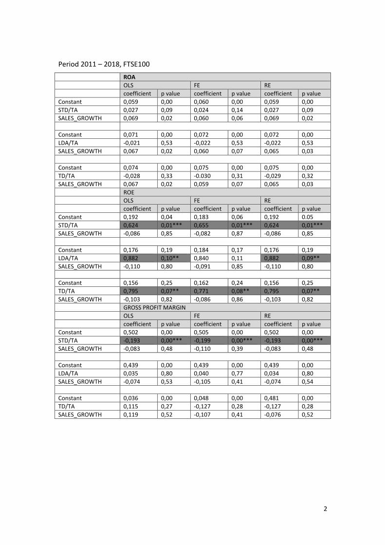
2
Period 2011 – 2018, FTSE100
ROA
OLS FE RE
coefficient p value coefficient p value coefficient p value
Constant 0,059 0,00 0,060 0,00 0,059 0,00
STD/TA 0,027 0,09 0,024 0,14 0,027 0,09
SALES_GROWTH 0,069 0,02 0,060 0,06 0,069 0,02
Constant 0,071 0,00 0,072 0,00 0,072 0,00
LDA/TA -0,021 0,53 -0,022 0,53 -0,022 0,53
SALES_GROWTH 0,067 0,02 0,060 0,07 0,065 0,03
Constant 0,074 0,00 0,075 0,00 0,075 0,00
TD/TA -0,028 0,33 -0.030 0,31 -0,029 0,32
SALES_GROWTH 0,067 0,02 0,059 0,07 0,065 0,03
ROE
OLS FE RE
coefficient p value coefficient p value coefficient p value
Constant 0,192 0,04 0,183 0,06 0,192 0.05
STD/TA 0,624 0,01*** 0,655 0,01*** 0,624 0,01***
SALES_GROWTH -0,086 0,85 -0,082 0,87 -0,086 0,85
Constant 0,176 0,19 0,184 0,17 0,176 0,19
LDA/TA 0,882 0,10** 0,840 0,11 0,882 0,09**
SALES_GROWTH -0,110 0,80 -0,091 0,85 -0,110 0,80
Constant 0,156 0,25 0,162 0,24 0,156 0,25
TD/TA 0,795 0,07** 0,771 0,08** 0,795 0,07**
SALES_GROWTH -0,103 0,82 -0,086 0,86 -0,103 0,82
GROSS PROFIT MARGIN
OLS FE RE
coefficient p value coefficient p value coefficient p value
Constant 0,502 0,00 0,505 0,00 0,502 0,00
STD/TA -0,193 0,00*** -0,199 0,00*** -0,193 0,00***
SALES_GROWTH -0,083 0,48 -0,110 0,39 -0,083 0,48
Constant 0,439 0,00 0,439 0,00 0,439 0,00
LDA/TA 0,035 0,80 0,040 0,77 0,034 0,80
SALES_GROWTH -0,074 0,53 -0,105 0,41 -0,074 0,54
Constant 0,036 0,00 0,048 0,00 0,481 0,00
TD/TA 0,115 0,27 -0,127 0,28 -0,127 0,28
SALES_GROWTH 0,119 0,52 -0,107 0,41 -0,076 0,52
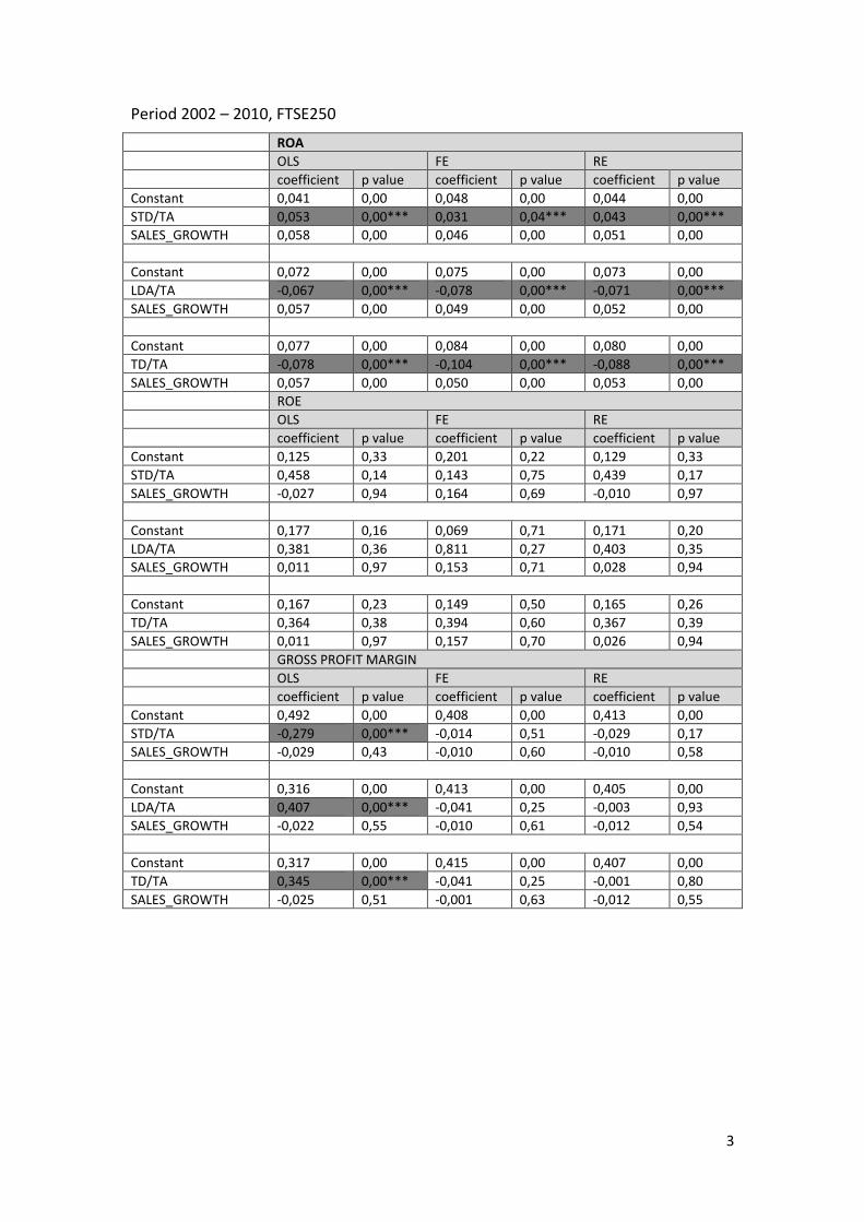
3
Period 2002 – 2010, FTSE250
ROA
OLS FE RE
coefficient p value coefficient p value coefficient p value
Constant 0,041 0,00 0,048 0,00 0,044 0,00
STD/TA 0,053 0,00*** 0,031 0,04*** 0,043 0,00***
SALES_GROWTH 0,058 0,00 0,046 0,00 0,051 0,00
Constant 0,072 0,00 0,075 0,00 0,073 0,00
LDA/TA -0,067 0,00*** -0,078 0,00*** -0,071 0,00***
SALES_GROWTH 0,057 0,00 0,049 0,00 0,052 0,00
Constant 0,077 0,00 0,084 0,00 0,080 0,00
TD/TA -0,078 0,00*** -0,104 0,00*** -0,088 0,00***
SALES_GROWTH 0,057 0,00 0,050 0,00 0,053 0,00
ROE
OLS FE RE
coefficient p value coefficient p value coefficient p value
Constant 0,125 0,33 0,201 0,22 0,129 0,33
STD/TA 0,458 0,14 0,143 0,75 0,439 0,17
SALES_GROWTH -0,027 0,94 0,164 0,69 -0,010 0,97
Constant 0,177 0,16 0,069 0,71 0,171 0,20
LDA/TA 0,381 0,36 0,811 0,27 0,403 0,35
SALES_GROWTH 0,011 0,97 0,153 0,71 0,028 0,94
Constant 0,167 0,23 0,149 0,50 0,165 0,26
TD/TA 0,364 0,38 0,394 0,60 0,367 0,39
SALES_GROWTH 0,011 0,97 0,157 0,70 0,026 0,94
GROSS PROFIT MARGIN
OLS FE RE
coefficient p value coefficient p value coefficient p value
Constant 0,492 0,00 0,408 0,00 0,413 0,00
STD/TA -0,279 0,00*** -0,014 0,51 -0,029 0,17
SALES_GROWTH -0,029 0,43 -0,010 0,60 -0,010 0,58
Constant 0,316 0,00 0,413 0,00 0,405 0,00
LDA/TA 0,407 0,00*** -0,041 0,25 -0,003 0,93
SALES_GROWTH -0,022 0,55 -0,010 0,61 -0,012 0,54
Constant 0,317 0,00 0,415 0,00 0,407 0,00
TD/TA 0,345 0,00*** -0,041 0,25 -0,001 0,80
SALES_GROWTH -0,025 0,51 -0,001 0,63 -0,012 0,55
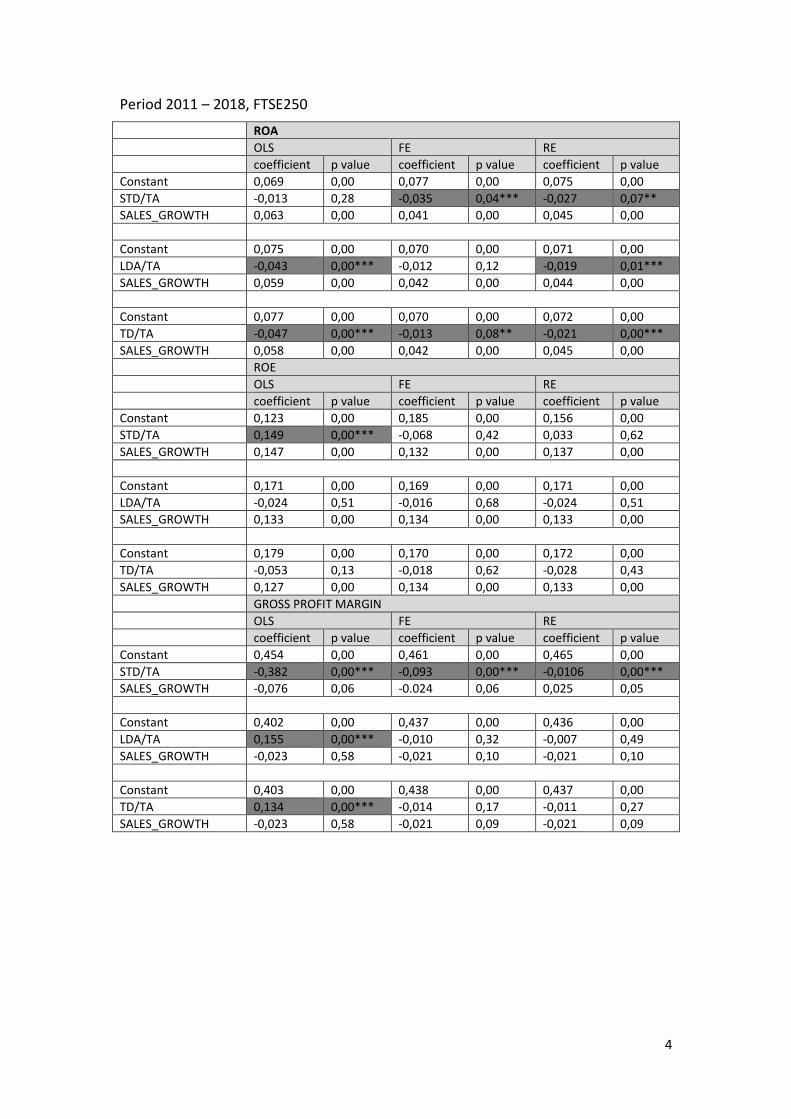
4
Period 2011 – 2018, FTSE250
ROA
OLS FE RE
coefficient p value coefficient p value coefficient p value
Constant 0,069 0,00 0,077 0,00 0,075 0,00
STD/TA -0,013 0,28 -0,035 0,04*** -0,027 0,07**
SALES_GROWTH 0,063 0,00 0,041 0,00 0,045 0,00
Constant 0,075 0,00 0,070 0,00 0,071 0,00
LDA/TA -0,043 0,00*** -0,012 0,12 -0,019 0,01***
SALES_GROWTH 0,059 0,00 0,042 0,00 0,044 0,00
Constant 0,077 0,00 0,070 0,00 0,072 0,00
TD/TA -0,047 0,00*** -0,013 0,08** -0,021 0,00***
SALES_GROWTH 0,058 0,00 0,042 0,00 0,045 0,00
ROE
OLS FE RE
coefficient p value coefficient p value coefficient p value
Constant 0,123 0,00 0,185 0,00 0,156 0,00
STD/TA 0,149 0,00*** -0,068 0,42 0,033 0,62
SALES_GROWTH 0,147 0,00 0,132 0,00 0,137 0,00
Constant 0,171 0,00 0,169 0,00 0,171 0,00
LDA/TA -0,024 0,51 -0,016 0,68 -0,024 0,51
SALES_GROWTH 0,133 0,00 0,134 0,00 0,133 0,00
Constant 0,179 0,00 0,170 0,00 0,172 0,00
TD/TA -0,053 0,13 -0,018 0,62 -0,028 0,43
SALES_GROWTH 0,127 0,00 0,134 0,00 0,133 0,00
GROSS PROFIT MARGIN
OLS FE RE
coefficient p value coefficient p value coefficient p value
Constant 0,454 0,00 0,461 0,00 0,465 0,00
STD/TA -0,382 0,00*** -0,093 0,00*** -0,0106 0,00***
SALES_GROWTH -0,076 0,06 -0.024 0,06 0,025 0,05
Constant 0,402 0,00 0,437 0,00 0,436 0,00
LDA/TA 0,155 0,00*** -0,010 0,32 -0,007 0,49
SALES_GROWTH -0,023 0,58 -0,021 0,10 -0,021 0,10
Constant 0,403 0,00 0,438 0,00 0,437 0,00
TD/TA 0,134 0,00*** -0,014 0,17 -0,011 0,27
SALES_GROWTH -0,023 0,58 -0,021 0,09 -0,021 0,09