the - iaria journals · rong zhao, detecon ... gerard damm, alcatel-lucent, france ... yu zheng,...

The International Journal on Advances in Telecommunications is Published by IARIA.

ISSN: 1942-2601

journals site: http://www.iariajournals.org

contact: [email protected]

Responsibility for the contents rests upon the authors and not upon IARIA, nor on IARIA volunteers,

staff, or contractors.

IARIA is the owner of the publication and of editorial aspects. IARIA reserves the right to update the

content for quality improvements.

Abstracting is permitted with credit to the source. Libraries are permitted to photocopy or print,

providing the reference is mentioned and that the resulting material is made available at no cost.

Reference should mention:

International Journal on Advances in Telecommunications, issn 1942-2601

vol. 2, no. 2&3, year 2009, http://www.iariajournals.org/telecommunications/

The copyright for each included paper belongs to the authors. Republishing of same material, by authors

or persons or organizations, is not allowed. Reprint rights can be granted by IARIA or by the authors, and

must include proper reference.

Reference to an article in the journal is as follows:

<Author list>, “<Article title>”

International Journal on Advances in Telecommunications, issn 1942-2601

vol. 2, no. 2&3, year 2009,<start page>:<end page> , http://www.iariajournals.org/telecommunications/

IARIA journals are made available for free, proving the appropriate references are made when their

content is used.

Sponsored by IARIA

www.iaria.org

Copyright © 2009 IARIA

International Journal on Advances in Telecommunications

Volume 2, Numbers 2&3, 2009

Editor-in-Chief

Tulin Atmaca, IT/Telecom&Management SudParis, France

Editorial Advisory Board

Michael D. Logothetis, University of Patras, Greece

Jose Neuman De Souza, Federal University of Ceara, Brazil

Eugen Borcoci, University "Politehnica" of Bucharest (UPB), Romania

Reijo Savola, VTT, Finland

Haibin Liu, Aerospace Engineering Consultation Center-Beijing, China

Advanced Telecommunications


Rui L.A. Aguiar, Universidade de Aveiro, Portugal


Symeon Chatzinotas, University of Surrey, UK

Denis Collange, Orange-ftgroup, France

Todor Cooklev, Indiana-Purdue University - Fort Wayne, USA

Jose Neuman De Souza, Federal University of Ceara, Brazil

Sorin Georgescu, Ericsson Research, Canada

Paul J. Geraci, Technology Survey Group, USA

Christos Grecos, University if Central Lancashire-Preston, UK

Manish Jain, Microsoft Research – Redmond

Michael D. Logothetis, University of Patras, Greece

Natarajan Meghanathan, Jackson State University, USA

Masaya Okada, ATR Knowledge Science Laboratories - Kyoto, Japan

Jacques Palicot, SUPELEC- Rennes, France

Gerard Parr, University of Ulster in Northern Ireland, UK

Maciej Piechowiak, Kazimierz Wielki University - Bydgoszcz, Poland

Dusan Radovic, TES Electronic Solutions - Stuttgart, Germany

Matthew Roughan, University of Adelaide, Australia

Sergei Semenov, Nokia Corporation, Finland

Carlos Becker Westphal, Federal University of Santa Catarina, Brazil

Rong Zhao, Detecon International GmbH - Bonn, Germany

Piotr Zwierzykowski, Poznan University of Technology, Poland

Digital Telecommunications

Bilal Al Momani, Cisco Systems, Ireland


Claus Bauer, Dolby Systems, USA

Claude Chaudet, ENST, France

Gerard Damm, Alcatel-Lucent, France

Michael Grottke, Universitat Erlangen-Nurnberg, Germany

Yuri Ivanov, Movidia Ltd. – Dublin, Ireland

Ousmane Kone, UPPA - University of Bordeaux, France

Wen-hsing Lai, National Kaohsiung First University of Science and Technology, Taiwan

Pascal Lorenz, University of Haute Alsace, France

Jan Lucenius, Helsinki University of Technology, Finland

Dario Maggiorini, University of Milano, Italy

Pubudu Pathirana, Deakin University, Australia

Mei-Ling Shyu, University of Miami, USA

Communication Theory, QoS and Reliability


Piotr Cholda, AGH University of Science and Technology - Krakow, Poland

Michel Diaz, LAAS, France

Ivan Gojmerac, Telecommunications Research Center Vienna (FTW), Austria

Patrick Gratz, University of Luxembourg, Luxembourg

Axel Kupper, Ludwig Maximilians University Munich, Germany

Michael Menth, University of Wuerzburg, Germany

Gianluca Reali, University of Perugia, Italy

Joel Rodriques, University of Beira Interior, Portugal

Zary Segall, University of Maryland, USA

Wireless and Mobile Communications

Tommi Aihkisalo, VTT Technical Research Center of Finland - Oulu, Finland

Zhiquan Bai, Shandong University - Jinan, P. R. China

David Boyle, University of Limerick, Ireland

Bezalel Gavish, Southern Methodist University - Dallas, USA

Xiang Gui, Massey University-Palmerston North, New Zealand

David Lozano, Telefonica Investigacion y Desarrollo (R&D), Spain

D. Manivannan (Mani), University of Kentucky - Lexington, USA

Himanshukumar Soni, G H Patel College of Engineering & Technology, India

Radu Stoleru, Texas A&M University, USA

Jose Villalon, University of Castilla La Mancha, Spain

Natalija Vlajic, York University, Canada

Xinbing Wang, Shanghai Jiaotong University, China

Ossama Younis, Telcordia Technologies, USA

Systems and Network Communications

Fernando Boronat, Integrated Management Coastal Research Institute, Spain

Anne-Marie Bosneag, Ericsson Ireland Research Centre, Ireland

Huaqun Guo, Institute for Infocomm Research, A*STAR, Singapore

Jong-Hyouk Lee, Sungkyunkwan University, Korea

Elizabeth I. Leonard, Naval Research Laboratory – Washington DC, USA

Sjouke Mauw, University of Luxembourg, Luxembourg

Reijo Savola, VTT, Finland

Multimedia

Dumitru Dan Burdescu, University of Craiova, Romania

Noel Crespi, Institut TELECOM SudParis-Evry, France

Mislav Grgic, University of Zagreb, Croatia

Christos Grecos, University of Central Lancashire, UK

Atsushi Koike, KDDI R&D Labs, Japan

Polychronis Koutsakis, McMaster University, Canada

Chung-Sheng Li, IBM Thomas J. Watson Research Center, USA

Artur R. Lugmayr, Tampere University of Technology, Finland

Parag S. Mogre, Technische Universitat Darmstadt, Germany

Chong Wah Ngo, University of Hong Kong, Hong Kong

Justin Zhan, Carnegie Mellon University, USA

Yu Zheng, Microsoft Research Asia - Beijing, China

Space Communications

Emmanuel Chaput, IRIT-CNRS, France

Alban Duverdier, CNES (French Space Agency) Paris, France

Istvan Frigyes, Budapest University of Technology and Economics, Hungary

Michael Hadjitheodosiou ITT AES & University of Maryland, USA

Mark A Johnson, The Aerospace Corporation, USA

Massimiliano Laddomada, Texas A&M University-Texarkana, USA

Haibin Liu, Aerospace Engineering Consultation Center-Beijing, China

Elena-Simona Lohan, Tampere University of Technology, Finland

Gerard Parr, University of Ulster-Coleraine, UK

Cathryn Peoples, University of Ulster-Coleraine, UK

Michael Sauer, Corning Incorporated/Corning R&D division, USA

International Journal on Advances in Telecommunications

Volume 2, Number 2&3, 2009

CONTENTS

Simple vehicle information delivery scheme for ITS networks

Katsuhiro Naito, Department of Electrical and Electronic Engineering, Mie University, Japan

Koushiro Sato, Department of Electrical and Electronic Engineering, Mie University, Japan

Kazuo Mori, Department of Electrical and Electronic Engineering, Mie University, Japan

Hideo Kobayashi, Department of Electrical and Electronic Engineering, Mie University, Japan

60 - 71

Escrow Serializability and Reconciliation in Mobile Computing using Semantic Properties

Fritz Laux, Fakultät Informatik, Reutlingen University, Germany

Tim Lessner, School of Computing, University of the West of Scotland, UK

72 - 87

A Family of Recursive Least-Squares Adaptive Algorithms Suitable for Fixed-Point

Implementation

Constantin Paleologu, Telecommunications Department, University Politehnica of Bucharest,

Romania

Silviu Ciochină, Telecommunications Department, University Politehnica of Bucharest, Romania

Andrei Alexandru Enescu, Telecommunications Department, University Politehnica of Bucharest,

Romania

88 - 97

Adaptive Rate Voice over IP Quality Management Algorithm

Eugene S. Myakotnykh, Norwegian University of Science and Technology, Norway

Richard A. Thompson, University of Pittsburgh, USA

98 - 110

60

International Journal on Advances in Telecommunications, vol 2 no 2&3, year 2009, http://www.iariajournals.org/telecommunications/

Simple vehicle information delivery scheme for ITS networks

Katsuhiro Naito, Koushiro Sato, Kazuo Mori, and Hideo KobayashiDepartment of Electrical and Electronic Engineering, Mie University,

1577 Kurimamachiya, Tsu, 514-8507, JapanEmail: {naito, kmori, koba}@elec.mie-u.ac.jp, [email protected]

Abstract— There has been significant interest and progress inthe field of vehicular ad hoc networks (VANETs) in recent years.Intelligent Transport System (ITS) is the major application ofVANETs. Vehicle-to-vehicle communication is an important fac-tor for safe driving applications such as blind crossing, preventionof collisions, and control of traffic flows. These applicationsrequire exchanges of vehicle information such as vehicle position,cruising speed, direction, and steering angle. Delivery schemes ofvehicle information require high delivery ratio, low latency, andhigh scalability. Additionally, large-size vehicles on actual roadenvironments may interrupt communication between vehicles.Therefore, adequate vehicles should forward vehicle informationto their neighbor vehicles in delivery of vehicle information. Thispaper proposes a new routing protocol for delivery of vehicleinformation to neighbor vehicles within a specified geographicalregion. The proposed protocol can deliver new vehicle informa-tion with short delay by performing temporal limited floodingbefore a route construction. Moreover, it can deliver vehicleinformation effectively with forwarding by adequate vehicles.As a result, our scheme can achieve the high delivery ratio ofvehicle information and high scalability. Finally, we assume thedifferent sizes of vehicles in the computer simulations. Then,we evaluate the proposed scheme in the more actual wirelessenvironment. The numerical results show that the proposedprotocol can achieve the high delivery ratio with short delayeven if the communication between standard-size vehicles isinterrupted by the large-size vehicle. Moreover, our protocol hasthe high scalability in case of increasing of vehicles.

Keywords— VANET, Vehicle-to-vehicle communication, ITSnetworks, Routing protocol, Vehicle information

I. I NTRODUCTION

Vehicular ad hoc networks (VANETs) are new technology tointegrate the capabilities of new wireless networks to vehicles.Intelligent Transport System (ITS) is the major application ofVANETs [2], [3], [4]. ITS includes several applications such asblind crossing, prevention of collisions, control of traffic flows,traffic monitoring, and nearby information services. Theseapplications can be divided into two major categories. Oneis called safety application, which improves vehicle safety onthe roads. The other is called user application, which providesvalue-added services such as internet access and entertainment.As for safety applications, their specification requires lowlatency, high delivery ratio, scalability, etc [5], [6]. VANETsare designed to provide drivers with real-time informationthrough vehicle-to-infrastructure communication or vehicle-to-vehicle communication.

The vehicle-to-infrastructure communication is used fordelivering of traffic information, electronic payment of high-way tolls, internet accesses, entertainment, etc [7]. Vehiclescommunicate with many base stations that are equipped alonga road. Therefore, vehicles perform handover of base stationsone after another. The vehicle-to-infrastructure communica-tion is especially important technology to achieve some userapplications in ITS. Meanwhile, vehicles communicate eachother in the vehicle-to-vehicle communication. Main serviceof vehicle-to-vehicle communication is offering vehicle infor-mation for safety applications.

The vehicle-to-vehicle communication in VANETs has spe-cial attributes that differentiate it from the other types ofnetworks such as mobile ad hoc networks (MANETs). One ofthe main different features between VANETs and MANETsis related to the behavior of nodes. Vehicles in VANETs arefaster than nodes in conventional MANETs. Moreover, themobility patterns of vehicles in VANETs are more restrictivedue to road structures. Therefore, these characteristics are veryeffective in most of the previous routing protocols [8].

Finding and maintaining routes has many difficulties in thedynamic behavior of vehicles in VANETs. Routing in VANETshas been recently studied and a variety of different protocolswere proposed [10]. These protocols can be classified into fivecategories such as pure ad-hoc routing, position-based routing,cluster-based routing, broadcast routing, and geocast routing.

VANETs and MANETs share the same principle such asself-organization, low bandwidth, and short radio transmissionrange. Therefore, most ad-hoc routing protocols are still ap-plicable. Ad-hoc on-demand distance vector (AODV) [11] anddynamic source routing (DSR) [12] are well-known routingprotocols for general purpose mobile ad-hoc networks. Theseprotocols can reduce overhead in scenarios with a small num-ber of flows. Meanwhile, VANETs differ from MANETs bytheir dynamic change of network topology. The conventionalstudies showed that most ad-hoc routing protocols suffer fromhighly dynamic nature of vehicle mobility and tend to havelow communication throughput due to poor route managementperformance [13].

Vehicle movement in VANETs is usually restricted in justbidirectional movements constrained along roads and streets[14]. Position-based routing employs routing strategies thatuse geographical information obtained from navigation system

61


on-board vehicles. Most position-based routing algorithms arebased on forwarding decision upon location information. Someprotocols exchange information of location and each vehicle’sspeed, and select a route with minimum link loss probability[15], [16], [17]. Additionally, greedy perimeter stateless rout-ing (GPSR) [18] is one of the well-known protocols. It worksbest in a free space scenario. However, direct communicationbetween vehicles may not exist due to buildings and large-sized vehicles. Connectivity-aware routing (CAR) protocolfinds paths between a source vehicle and a destination vehicle,considering vehicle traffic and movement of vehicles [19].

In cluster-based routing, each cluster can have a clusterhead, which is responsible for intra- and inter-cluster commu-nication [20]. Vehicles in a cluster communicate with neighborvehicles directly. Inter-cluster communication is performedvia the cluster-heads. Many cluster-based routing protocolshave been proposed in MANETs. However, the VANETshave different features due to constraints on mobility, highspeed movement, and driver behavior. As a result, cluster-based routing protocols can achieve good scalability for largenetworks. But, vehicles suffer from the long delay and theoverhead involved in forming and maintaining clusters inVANETs [21].

Broadcast routing is frequently used for delivering adver-tisements and announcements in VANETs. The simplest wayto implement broadcast mechanisms is flooding, in which eachvehicle re-broadcasts packets to all of its neighbors. Floodingperforms relatively well for a small number of vehicles.However, it suffers from broadcast storm problems when thenumber of vehicle in networks increases [22]. Some schemesfor the broadcast storm problems have been proposed in ad hocnetworks [23], [24], [25]. However, the investigation about thebroadcast storm problems is not enough to be considered inVANETs.

Geocast routing is a location-based multicast routing [26].Therefore, packets are delivered from a source vehicle toall other vehicles with a specified geographical region. Thegeocast routing is benefit mechanisms in many applications ofVANETs. For example, a vehicle can detect some problems inneighbor vehicles to prevent collisions. Most geocast routingschemes are based on directed flooding. In VANETs, eachvehicle can obtain its own location by using global positioningsystem (GPS). Therefore, some researchers have proposedforwarding techniques that reduce redundant transmission byusing this location information [27], [28].

However, almost all schemes do not consider intercept ofcommunication by large-size vehicle. In the actual VANETs,sizes of vehicles are also different. Therefore, VANET routingprotocols should consider the actual communication environ-ment. Another researcher considers broadcast schemes basedon IEEE 802.11 [29], [30]. In these techniques, adequatevehicles for forwarding are selected because vehicle positions

Source Vehicle

SV1

SV2

SV3 SV4

SV5

LV1

LV2

Forwarder vehicle for SV1

Forwarder vehicle for SV4 & SV5

Fig. 1. Vehicle information delivery in ITS.

are exchanged via some control packets. However, actualwireless environments in ITS networks are especially severefrom a practical standpoint. For examples, a standard-sizedvehicle comes under an influence of blocking by large-sizevehicles, and each vehicle suffers from dynamic fluctuationof signal intensity by moving so fast. In these environments,a distance can not be appropriate criteria for selection offorwarder vehicles.

We have proposed a simple delivery scheme for vehicleinformation [1]. In this paper, we evaluate packet deliveryratio and transmission delay. One characteristic of our schemeis utilizing vehicle information messages (VIMs) themselvesfor route construction. At first phase, all vehicles forward allvehicle information messages on a temporary basis. Therefore,delivery of new vehicle information can be achieved withshort delay. This characteristic will be especially important toachieve blind crossing and prevention of collisions The reasonfor this is that almost all routing protocols require several pe-riods to construct routes, and these route construction periodswill have big overhead to reduce the delay for recognizingeach vehicle. At second phase, each vehicle selects an adequateforwarder vehicle for its vehicle information forwarding. As aresult, the number of forwarded vehicle information messagescan be reduced to solve broadcast storm problems. Thischaracteristic is an important factor to achieve high scalabilitywith increasing of vehicles. Finally, our scheme utilizes vehicleinformation instead of hello messages to maintain routes.Consequently, our scheme can check a link status betweenneighbor vehicles without any control messages, and thenumber of control messages can be also reduced. We assumethe different sizes of vehicles in the computer simulations.Then, we evaluate the proposed scheme in the more actualwireless environment. The numerical results show that theproposed scheme can achieve the high delivery ratio with shortdelivery delay.

II. SYSTEM MODEL

A purpose of this paper is to achieve a vehicle-to-vehiclecommunication scheme, which delivers vehicle informationwithin a specified geographical region. Figure 1 is a di-agrammatic illustration of vehicle information delivery forsafety applications in VANETs. We assume that each vehicletransmits its vehicle information message as a source vehicle

62


Source Vehicle

SV3 SV4

SV5LV2 SV6

Delivery area of Source vehicleFRM

FRMChanges to Forwarder SV5

Fig. 2. Example procedure of forwarding request.

Source Vehicle

SV3 SV4

SV5LV2 SV6

Delivery area of Source vehicle

FSM

Distance > threshold

Temporal forwarding is acctivated

Fig. 3. Example procedure of forwarder search request.

periodically. But, we focus our attention on routes to neighborvehicles from a source vehicle in Fig. 1. VehiclesSV 2 andLV 2 are forwarder vehicles for their neighbor vehicles. Ourprotocol can support a mixed environment of standard-sizedand large-size vehicles. A vehicle information message isdelivered to some vehicles in a limited area. The limited areais defined as the delivery distance, and is determined as afixed value beforehand. Our scheme can be implemented in abidirectional road environment by using directional informa-tion of vehicles. However, we assume a one-way road in theexplanation for simplicity.

In the proposed protocol, three types of control messagesare introduced to deliver vehicle information messages; aForwarding Request Message (FRM), a Forwarder SearchMessage (FSM), and a Forwarding Abort Message (FAM). TheFRM is transmitted when vehicles request neighbor vehiclesto activate forwarding function. The FSM is transmitted whenvehicles detect link losses. The FAM is transmitted when adistance between a vehicle and its source vehicle is longer thanits delivery distance. These example procedures are shown inFigures 2, 3 and 4.

Almost all routing protocols require periodic transmissionof control packets because adequate routes may be changeddue to moving of vehicles. On the contrary, each vehicle doesnot transmit the control packets periodically in the proposedprotocol. In order to recognize neighbor vehicles, each vehicleuses vehicle information messages as substitutes for specialcontrol packets like hello messages. As a result, controlmessages are only transmitted when vehicles lose links toneighbor vehicles or change links to other neighbor vehicles.Therefore, our protocol can reduce the number of transmittedcontrol messages.

Table I shows the components of the routing table. In theproposed scheme, the routing table in Table I is constructedfor each source vehicle. In the assumed ITS networks, vehicle

Source Vehicle

SV3 SV4

SV5LV2 SV6

Delivery area of Source vehicle

FAM

Fig. 4. Example procedure of forwarding abort request.

Source Vehicle

SV1

SV2

SV3

SV4 SV5LV1

LV2 SV6

Source vehicle ID : SV2Forwarder’ s vehicle ID : SV3Forwarding requested vehicle IDs : SV5, SV6

Fig. 5. Example routing information of LV2.

information is delivered in a limited area near a source vehicle.Therefore, our assumed application is one of multicast applica-tion types and the proposed protocol is one of geocast routingprotocols. As a result, each source vehicle has a receiver groupfor vehicle information. In the proposed protocol, the sourcevehicle ID is used for determining the receiver group for thesource vehicle. The source vehicle position is used to detect thedelivery area. The final received time of vehicle informationis used to remove the routing information if the vehicle doesnot receive the vehicle information for a long time. Theforwarder’s vehicle ID is used to maintain its own forwardervehicle information. The forwarding requested vehicles IDsare an ID list of vehicles, which transmit a Forwarding RequestMessage to its own vehicle. If this list has some vehicle IDs,the vehicle should forward vehicle information from the sourcevehicle. The forwarding requested vehicle positions are listsof positions for forwarding requested vehicles. These lists areused to find vehicles that exist outside of delivery area of thesource vehicle.

Figure 5 is example routing information of large-size vehicle2. The LV2 has constructed a route to the SV3 and has beenrequested to forward vehicle information of the SV2 by theSV5 and the SV6. Therefore, the forwarder’s vehicle ID ofLV2 is the SV3, and the forwarding requested vehicles IDsare SV5 and SV6.

Figure 6 shows a flow chart of the proposed routing scheme.In this flow chart, a source vehicleS transmits a vehicleinformation message periodically, and a forwarder vehicleF

forwards the vehicle information message from the vehicleS.Finally, a destination vehicleD receives it.

63


If Vehicle D is in the delivery area of Vehicle S ?

If the vehicle information about Vehicle S is registered in

routing table of the vehicle ?

If the distance between Vehicle F and D is less than

the threshold ?

If Vehicle D is forwarding vehicle for

Vehicle S ?OR

If the counter for temporal forwarding

> 0 ?

Receive a vehicle information about Vehicle S from Vehicle F

Transmit a Forwarding Abort Messagefor vehicle information of Vehicle S

Add a vehicle ID of Vehicle F, a vehicle ID and a location of Vehicle S into the routing table

Transmit a Forwarding Request Message of Vehicle S

Transmit a Forwarder Search Messagefor vehicle information of Vehicle S

Yes

Yes

Yes

No No

No

Abort the transmission

Receive the Forwarder Search Messagefor vehicle information of Vehicle S from Vehicle D

Set the counter for temporal forwarding to the maximum transmission number

Receive the Forwarding Abort Messagefor vehicle information of Vehicle S from Vehicle D

Remove the forwarding information of Vehicle S for Vehicle D

Forward the vehicle information of Vehicle S,The counter for temporal forwarding -- ,Restart timer for maintain routing table

Receive the Forwarder Search Messagefor vehicle information of Vehicle S from Vehicle D

Add a vehicle ID of Vehicle S, a vehicle ID and a location of Vehicle D into the routing table

Vehicle Information Message

Forwarding Request Message Forwarder Search Message

Yes

No

Forwarding Abort Message

Fig. 6. Flow chart of the proposed routing protocol.

A. Forwarding Procedures

When a vehicle receives new vehicle information messagesfrom neighbor vehicles, two procedures will be performed.The first one is forwarding procedures and the second one isforwarding request procedures. In the forwarding procedures,vehicles forward the received vehicle information message toneighbor vehicles. The procedures are described as follows.

1) The vehicle calculates a distance between a previous hopvehicle and itself.

2) The vehicle calculates a forwarding delay period accord-ing to the distance in order to set priorities of forwarding.The delay period is set to a short time when the distanceis long. On the contrary, the delay period is set to along time when the distance is short. This is because the

64


TABLE I

COMPONENTS OF ROUTING TABLE.

Source vehicle IDSource vehicle positionFinal received time of vehicle information from source vehicleForwarder’s vehicle IDForwarding requested vehicle IDsForwarding requested vehicle positions

number of hops can be reduced if the distance is long. Inthe proposed procedures, every vehicle forward vehicleinformation with prioritized delay on a temporary basis.Therefore, the proposed scheme is tolerant of vehiclemovement.

3) The vehicle sets a forwarding delay period that is relatedto the distance.

4) The vehicle forwards the received vehicle informationmessage with this forwarding delay period.

B. Forwarding Request Procedures

In the forwarding request procedures, vehicles request toforward vehicle information messages to neighbor vehicles.Procedures are described as follows.

1) The vehicle calculates the distance between the sourcevehicle of the vehicle information message and itself.

2) The vehicle checks the routing table to find the sourcevehicle ID within the vehicle information message whenthe distance is shorter than the delivery distance.

3) The vehicle adds the vehicle ID and a position of thesource vehicle into the routing table when the sourcevehicle ID cannot be found in the routing table.

4) The vehicle requests the previous hop vehicle as aforwarder vehicle for itself by transmitting a ForwardingRequest Message (FRM).

5) The neighbor vehicle that receives the FRM adds avehicle ID and a vehicle position of the requestingvehicle.

6) The neighbor vehicle starts forwarding of vehicle infor-mation messages to the requesting vehicle.

Figure 2 is an example procedure when the vehiclesSV 4andSV 5 transmit FRMs. In this figure, the vehicleSV 6 doesnot transmit a FRM because it exists outside of delivery areaof the source vehicleSV 0. Finally, the vehicleLV 2 startsforwarding of new vehicle information messages.

C. Forwarder Search Procedures

Following procedures are performed when the distancebetween a forwarder vehicle and itself becomes longer than athreshold.

1) The vehicle tries to find another vehicle as a forwardervehicle because the current forwarder vehicle is far fromitself.

2) The vehicle transmits a Forwarder Search Message(FSM) to neighbor vehicles.

3) The neighbor vehicles activate each forwarding functionof vehicle information messages if each distance be-tween the vehicle transmitting the FSM and themselvesis shorter than the threshold.

4) The neighbor vehicles start forwarding their vehicleinformation messages for a while. The maximum re-transmission time of vehicle information messages is setto a counter for the temporal forwarding.

5) The vehicle transmits a new FRM to an adequate vehicleof its neighbor vehicles when it receives a new vehicleinformation message from them.

Figure 3 is an example procedure when the vehicleSV 5transmits a FSM because the distance between theLV 2 andtheSV 5 is longer than the threshold. In this figure, the vehicleSV 4 activates the temporal forwarding procedures for theSV 5. Hence, the vehicleSV 5 will transmit a FRM to thevehicleSV 4.

D. Forwarding Abort Procedures

Following procedures are performed when vehicles move tooutside of the delivery area of their source vehicle

1) The vehicle transmits a Forwarding Abort Message(FAM) to its forwarder vehicle.

2) The forwarder vehicle removes the forwarding informa-tion for it from the routing table.

Figure 4 is an example procedure when the vehicleSV 5moves to outside of the delivery area, and transmits a FAMto the vehicleSV 4. The vehicleSV 4 will inactivate theforwarding procedures for the vehicleSV 5.

III. E XAMPLE OPERATIONS

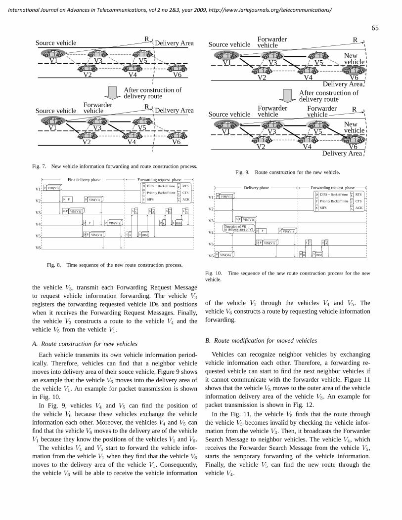
In the proposed scheme, each vehicle starts to construct aroute by receiving a new vehicle information. In this section,we explain example operations of the proposed scheme withthe vehicle layout in Fig. 7. Figure 8 shows an example ofpacket transmission in this situation. In the example, eachvehicle is assumed to deliver vehicle information within radiusR.

In Fig. 7, the vehicleV1 is regarded as a source vehicle.The vehiclesV2, V3, V4, and V5 exist in the area where thevehicle information of the vehicleV1 can be delivered. ThevehicleV1 transmits the vehicle information messages (VIMs)periodically. The neighbor vehiclesV2 and V3 register thenew vehicleV1 by checking each routing table. Then, eachvehicle calculates a forwarding delay according to relativeposition to the source vehicleV1. The vehicleV3 sets a shorterdelay than the vehicleV2 because the relative position toV3 is longer than that ofV2. This procedure reduces thehop count for vehicle information delivery. Then, vehiclesV4

and V5, which receive the vehicle information forwarded by

65


Source vehicle

V1

V2

V3

V4

V5

V6

RDelivery Area

After construction ofdelivery route

Delivery AreaRSource vehicle

Forwarder vehicle

V1

V2

V3

V4

V5

V6

Fig. 7. New vehicle information forwarding and route construction process.

V1

V2

V3

V4

V5

V6

D

FRMR

C A

P

P

D

D

PD

PD

D

D

D

S S

FRMRD S

C AS S

First delivery phase Forwarding request phase

VIM (V1)

VIM (V1)

VIM (V1)

VIM (V1)

VIM (V1)

D

P

S

DIFS + Backoff time

Priority Backoff time

SIFS

R

C

A

RTS

CTS

ACK

S

Fig. 8. Time sequence of the new route construction process.

the vehicleV3, transmit each Forwarding Request Messageto request vehicle information forwarding. The vehicleV3

registers the forwarding requested vehicle IDs and positionswhen it receives the Forwarding Request Messages. Finally,the vehicleV3 constructs a route to the vehicleV4 and thevehicleV5 from the vehicleV1.

A. Route construction for new vehicles

Each vehicle transmits its own vehicle information period-ically. Therefore, vehicles can find that a neighbor vehiclemoves into delivery area of their souce vehicle. Figure 9 showsan example that the vehicleV6 moves into the delivery area ofthe vehicleV1. An example for packet transmission is shownin Fig. 10.

In Fig. 9, vehiclesV4 and V5 can find the position ofthe vehicleV6 because these vehicles exchange the vehicleinformation each other. Moreover, the vehiclesV4 andV5 canfind that the vehicleV6 moves to the delivery are of the vehicleV1 because they know the positions of the vehiclesV1 andV6.

The vehiclesV4 and V5 start to forward the vehicle infor-mation from the vehicleV1 when they find that the vehicleV6

moves to the delivery area of the vehicleV1. Consequently,the vehicleV6 will be able to receive the vehicle information

Forwarder vehicleSource vehicle

V 1

V 2

V 3

V 4

V 5

V 6

R

Delivery AreaAfter construction ofdelivery route

Delivery Area

RSource vehicle

Forwarder vehicle

V 1

V 2

V 3

V 4

V 5

V 6

Forwarder vehicle

Newvehicle

Newvehicle

Fig. 9. Route construction for the new vehicle.

V1

V2

V3

V4

V5

V6

D VIM (V1)

PD

PD

PD

FRMRD S

C AS S

Delivery phase Forwarding request phase

D VIM (V6)

VIM (V1)

VIM (V1)

D VIM (V1)

Detection of V6in delivery area of V1

D

P

S

DIFS + Backoff time


SIFS

R

C

A

RTS

CTS

ACK

Fig. 10. Time sequence of the new route construction process for the newvehicle.

of the vehicle V1 through the vehiclesV4 and V5. ThevehicleV6 constructs a route by requesting vehicle informationforwarding.

B. Route modification for moved vehicles

Vehicles can recognize neighbor vehicles by exchangingvehicle information each other. Therefore, a forwarding re-quested vehicle can start to find the next neighbor vehicles ifit cannot communicate with the forwarder vehicle. Figure 11shows that the vehicleV5 moves to the outer area of the vehicleinformation delivery area of the vehicleV3. An example forpacket transmission is shown in Fig. 12.

In the Fig. 11, the vehicleV5 finds that the route throughthe vehicleV3 becomes invalid by checking the vehicle infor-mation from the vehicleV3. Then, it broadcasts the ForwarderSearch Message to neighbor vehicles. The vehicleV4, whichreceives the Forwarder Search Message from the vehicleV5,starts the temporary forwarding of the vehicle information.Finally, the vehicleV5 can find the new route through thevehicleV4.

66


Forwarder vehicleSource vehicle

V 1

V 2

V 3

V 4

V 5

V 6

RDelivery Area

After reconstruction ofdelivery route

Delivery AreaRSource vehicle

Forwarder vehicle

V 1

V 2

V 3

V 4

V 5

V 6

Slowvehicle

Slowvehicle

Forwarder vehicle

Fig. 11. Route modification process.

V1

V2

V3

V4

V5

V6

D VIM (V1)

FSM FRMRD S

C AS S

Delivery timeoutphase Forwarder search phase

D VIM (V1)

D

D VIM (V1)

D VIM (V1)

Forwarding request phase

D

P

S

DIFS + Backoff time


SIFS

R

C

A

RTS

CTS

ACK

Fig. 12. Time sequence of the route modification process.

C. Route discard for moved vehicles

In the proposed scheme, two procedures for route discardare considered. The first is used in a situation that vehiclesin a certain delivery area cannot receive any information of avehicle, which were in the area, and they cannot recognize itany more. The second is used in a situation that vehicles ina certain delivery area can receive information of a vehicleand can recognize it, but it is moving out to the area. Inthe situations, they discards the routes in their own routingtable. Figure 13 shows an example that the vehicleV5 movesto the outer area of the vehicle information delivery areaof the vehicleV1. Figure 14 shows an example for packettransmission in this situation.

The vehicleV5 uses the route through the vehicleV4 in Fig.13. It transmits a Forwarding Abort Message to the vehicleV4

if it exists in the outer area of delivery area for a given lengthof time. Finally, the vehicleV4 stops vehicle informationforwarding and removes the route for the vehicleV5.

IV. N UMERICAL RESULTS

In order to evaluate the feasibility of the proposed scheme,we performed computer simulations with network simulatorQualNet [31]. Qualnet is the well-known wireless network

Source vehicle

V1

V2

V3

V4

V5

V6

RDelivery Area

After elimination ofdelivery route

Delivery AreaR

Source vehicleForwarder vehicle

V1

V2

V3

V4

V5

V6

Slowvehicle

Slowvehicle

Forwarder vehicle

Forwarder vehicle

Fig. 13. Route discard process.

V1

V2

V3

V4

V5

V6

FAMRD S

C AS S

Checking phase for outer delivery area of V1

D

outer delivery area of V1VIM (V1)

D VIM (V1)

D VIM (V1)

Forwarding Abort phase

D

P

S

DIFS + Backoff time


SIFS

R

C

A

RTS

CTS

ACK

Fig. 14. Time sequence of the route discard process.

simulation software that considers the more actual wireless en-vironment. Therefore, packet errors are handled as the packeterror ratio according to the received signal-to-interference andnoise power ratio (SINR). Each results shows an average of10 trials of simulation. Our proposed protocol is one of theinformation delivery schemes by broadcast communication. Itis known that broadcast communication suffers from packetcollisions when many vehicles exist in a communication area.Therefore, we considered 50 vehicles for small number ofvehicles and 200 vehicles for large number of vehicles. Weassumed that a road shape is a loop line with a radius equalsto 1500 [m] and 2 lanes. Each vehicle is located randomly onthe road, selecting the velocity between 90 [km/h] and 110[km/h] randomly. Therefore, a distribution of vehicle velocityis uniformly between 90 [km/h] and 110 [km/h] The vehicleruns on the inside lane principally and keeps an inter-vehiculardistance as 100 [m]. If there is no vehicle on the outside lane,the vehicle moves to the outside lane from the inside laneto overtake a forward vehicle. After overtaking, the vehiclemoves to the inside lane if there is no vehicle on the insidelane. In the simulations, about 50 times of passing occur when

67


TABLE II

SIMULATION PARAMETERS.

Simulator QualNetSimulation time 150 [s]Simulation trial 10 [times]Number of vehicles 50, 200 [vehicles]Vehicle velocity 90 – 110 [km/h]Size of vehicle information message 100 [Byes]Transmission interval 250 [ms]Communication device IEEE 802.11bTransmission rates 11 [Mbps]Transmission power 15 [dBm]Antenna gain 0 [dB]Antenna type Omni directionalAntenna height 1.5 [m]Propagation path loss model Two rayWireless environment AWGNRoad shape Circle with radius = 1500 [m]Number of lanes 2 [lanes]

the number of vehicle is 50, and about 150 times of passingoccur when the number of vehicle is 200. Finally, the featureof this paper is to consider the effect of large-size vehicles.So, we define the large-size vehicle ratio that means the ratioof the large-size vehicles and the standard-size vehicles. Whenthe large-size vehicle ratio is set to 0, all vehicles are standard-size vehicles.

As the wireless propagation model, we used a two ray prop-agation model. Moreover, we consider blocking effects dueto large-size vehicles. So, we assumed that large-size vehiclesare rectangular solids. If a rectangular solid is overlapped withthe straight line between two standard-size vehicles, these twovehicles cannot communicate due to blocking.

The final purpose of this study is to fuse vehicle informationdelivery and communication networks for several networkapplications. Therefore, we employ IEEE 802.11b for a com-mon comunication device. In the simulations, the transmissionrange is about 500 [m], packet errors are determined dueto the received signal-to-interference and noise power ratio(SINR). Our packet error model can consider packet collisionsand noises. The size of a vehicle information message is 100[Byte], and is transmitted with 4 [packets/s]. The delivery areaof vehicle information messages is assumed to be 1000 [m].

Our protocol is one of the broadcast communication meth-ods. Therefore, we employ the probabilistic flooding schemefor comparison. The flooding probability is assumed to be 0,25, 50, 75, 100 [%]. Simulation parameters are shown in detailin Table II.

Figure 15 shows the delivery ratio of vehicle informationmessages with 50 vehicles. In this study, we define that thedelivery ratio is the message received ratio for vehicles in thedelivery area. From results, we can find that our proposedprotocol can achieve the highest delivery ratio. The deliveryratio of the probabilistic flooding scheme degrades when the

0

0.2

0.4

0.6

0.8

1

0 0.25 0.5 0.75 1

Del

iver

y R

atio

Large-size Vehicle Ratio

ProposedFlooding with P=100%Flooding with P=75%Flooding with P=50%Flooding with P=25%

P=25%

P=50%

P=75%

P=100%

Fig. 15. Delivery ratio of vehicle information (50 vehicles).

0

0.2

0.4

0.6

0.8

1

0 0.25 0.5 0.75 1

Del

iver

y R

atio



P=25%

P=50%

P=75%

P=100%

Fig. 16. Delivery ratio of vehicle information (200 vehicles).

flooding probability decreases. This is because several vehiclesare required to forward vehicle information messages whenthere are a small number of vehicles on the road. Moreover,the delivery ratio of all schemes degrades when the large-sizevehicle ratio increases. Especially, it degrades much when thevalue of the flooding probability is set low. The reason forthis is that large-size vehicles block communications betweenstandard-size vehicles. So, more vehicles should be requiredto forward vehicle information messages.

Figure 16 shows the delivery ratio of vehicle informationmessages with 200 vehicles. From results, our proposed pro-tocol can keep the highest delivery ratio. But, the deliveryratio of the flooding scheme degrades. This is because theflooding schemes suffer from broadcast storm problems. Wecan find that some flooding schemes can achieve good deliveryratio. However, the optimum flooding probability is alsochangeable depending on situation change. So, it is difficult toselect the optimum flooding probability in the actual system.

68


0

10

20

30

40

50

0 0.25 0.5 0.75 1

Num

ber

of fo

rwar

ded

vehi

cle

info

rmat

ion



P=25%

P=50%

P=75%

P=100%

Fig. 17. Number of forwarded vehicle information (50 vehicles).

0

10

20

30

40

50

0 0.25 0.5 0.75 1

Num

ber

of fo

rwar

ded

vehi

cle

info

rmat

ion


Proposed

Flooding with P=100%

Flooding with P=75%

Flooding with P=50%

Flooding with P=25%

Fig. 18. Number of forwarded vehicle information (200 vehicles).

Incidentally, the delivery ratio of the proposed protocol canachieve high performance even if the large-size vehicle ratio ischanged because each vehicle selects an optimum vehicle as itsforwarder vehicle in the proposed protocol. In the conventionalresearch, the objective packet delivery ratio is assumed tobe 90 [%]. In the broadcast communication, packets may becorrupted due to hidden terminal problems. Therefore, it isdifficult to achieve high delivery ratio when special mediaaccess control (MAC) method is not employed. In our deliveryratio, we evaluate packet delivery ratios at all receiver vehicles.Therefore, we think that our protocol can be used for the actualenvironments by employing the Forward Error Correction(FEC).

Figure 17 shows the number of forwarded vehicle informa-tion in the delivery area with 50 vehicles. From results, wecan find that the flooding schemes require several times offorwarding. Therefore, the flooding schemes can achieve highdelivery performance. However, these excess forwarding are

0

5

10

15

20

25

0 0.25 0.5 0.75 1

Tra

nsm

issi

on d

elay

[ms]



P=25%

P=50%

P=75%

P=100%

Fig. 19. Delay performance (50 vehicles).

0

50

100

150

200

250

0 0.25 0.5 0.75 1

Tra

nsm

issi

on d

elay

[ms]



P=25%

P=50%

P=75%

P=100%

Fig. 20. Delay performance (200 vehicles).

unreasonable from the viewpoint of the wireless resource. Theprobabilistic flooding can decrease the number of forwarding.But, the delivery ratio is also degraded. On the contrary,our proposed protocol requires small number of forwardinglike the probabilistic flooding with 25 [%]. However, theproposed protocol can achieve the high delivery ratio like thefull flooding scheme. Therefore, our protocol is a reasonablescheme from the viewpoint of wireless resources.

Figure 18 shows the number of forwarded vehicle informa-tion in the delivery area with 200 vehicles. From results, theperformance of the probabilistic flooding with 25 [%] keepssmall number of forwarded vehicle information messages.However, the delivery ratio of the probabilistic flooding with25 [%] degrades due to blocking by large-size vehicles. This isbecause it is difficult to forward vehicle information messageappropriately when the flooding probability decreases. Mean-while, the proposed protocol can keep the smallest numberof forwarded vehicle information messages. Moreover, the

69


2

4

6

8

10

12

14

16

18

20

22

0 0.2 0.4 0.6 0.8 1

Del

ay [m

s]

Large-siz e V eh ic le R atio

Large-siz e V eh ic les

Stand ard -siz e V eh ic les

Fig. 21. Delay performance of standard and large-size vehicles.

performance of the proposed protocol achieves a stable de-livery ratio and a stable forwarding performance because eachvehicle selects its forwarder vehicle by considering blockingdue to large-size vehicles.

Figure 19 shows the delay performance with 50 vehicles.The delay period starts when a source vehicle transmitsa vehicle information message, and ends when the vehicleinformation message is received at all vehicles in the deliveryarea. Therefore, the accurate delay of each vehicle is differentdue to the positions of the vehicles. So, the delay performanceaverages delays of all vehicles in the delivery area. Fromresults, the delay performance of the proposed protocol isa little shorter than that of the full flooding scheme. Thedelay performance of all schemes increases when the large-size vehicle ratio increases. The reason for this is that blockingby the large-size vehicles causes degradation of the actualtransmission range. Therefore, more forwarder vehicles arerequired to transmit the vehicle information messages.

Figure 20 shows the delay performance with 200 vehicles.From results, the delay performance of the proposed proto-col can keep short values when the large-size vehicle ratiochanges. On the contrary, the flooding schemes have especiallylong delay when the large-size vehicle ratio equals to 0 or 100[%]. The actual transmission range becomes long when there isno effect of blocking due to the large-size vehicles. Therefore,broadcast storm problems occur.

Figure 21 shows the delay performance of standard-size andlarge-size vehicles in the proposed protocol. This kind of delayis required to transmit vehicle information in MAC layer. Fromresults, we can find that delays of large-size vehicles decreaseaccording to increasing of the large-size vehicle ratio becauselarge-size vehicles block communications between standard-size vehicles and the number of vehicles in a certain communi-cation area also decreases. Therefore, each vehicle can obtainmore opportunities to transmit vehicle information. On the

0

0.2

0.4

0.6

0.8

1

50 100 150 200

De

live

ry R

atio

Number of Vehicles

Proposed

Flooding with P = 100%




Fig. 22. Delivery ratio of vehicle information (large-size vehicle:40[%].

contrary, the delay performance of large-size vehicles is alsoconstant. This is because large-size vehicles can communicatewith standard-size vehicles and large-size vehicles. Moreover,these communication are not blocked. Then, the number ofvehicles sharing the same communication is also increasing.As a result, it is difficult for large-size vehicles to obtainopportunities to transmit vehicle information.

Figure 22 shows the delivery ratio of vehicle informationwith a large-size vehicle ratio equals to 40 [%] and 200vehicles. From results, the performance of the all floodingmechanisms degraded according to increasing in the numberof vehicles. The reason for this is that it is difficult to selectadequate forwarding vehicles in the situation the large-sizevehicle ratio equals to 40 [%]. Meanwhile, the proposedprotocol has good scalability performance. The scalability isone of the most important factor in ITS. This is becausethe proposed protocol is especially simple and only a fewcontrol messages are exchanged when a vehicle joins certainnetworks, it changes its forwarding vehicle and drops outthe networks. Moreover, the proposed protocol can select anadequate forwarding vehicle, and improve effectiveness ofchannel resource.

Figure 23 shows the number of forwarded vehicle informa-tion with a large-size vehicle ratio equals to 40 [%] and 200vehicles. From results, we can find that the proposed protocolcan keep a small number of forwarded vehicle information.However, the performance of the proposed protocol is littlelarger than that of the probabilistic flooding with P = 25[%] because the proposed protocol can select the forwardingvehicles. Therefore, more vehicles are selected as a forward-ing vehicle when large-size vehicles blocks communicationbetween standard-size vehicles.

Figure 24 shows the delay performance with a large-sizevehicle ratio equals to 40 [%] and 200 vehicles. From results,the delay performance degrades according to increasing in the

70


0

5

10

15

20

25

30

35

40

45

50

50 100 150 200Nu

mb

er

of fo

rwa

rde

d v

eh

icle

in

form

atio

n

Number of Vehicles

Proposed

Flooding

Flooding with Probability : 75%



Fig. 23. Number of forwarded vehicle information (large-size vehicle:40[%].

0

20

40

60

80

100

120

140

160

50 100 150 200

De

lay [m

s]

Number of Vehicles

Proposed





Fig. 24. Delay performance (Big size vehicle:40[%]).

flooding probability. This is because broadcast storms occurand it is difficult for almost all vehicles to transmit vehicleinformation. On the contrary, the proposed protocol can keepthe short delay even if the number of vehicle increases.

Figure 25 shows the continuous drop ratio of vehicleinformation with a large-size vehicle ratio equals to 40 [%]and 200 vehicles. The continuous drop ratio means the ratiothat the vehicle cannot receive the vehicle information contin-uously. The continuous drops of vehicle information are notsuited characteristics for ITS communication because thesedrops cause temporal interruption of communication betweenneighbor vehicles. From results, we can find that the proposedprotocol has good tolerance to burst packet losses.

V. CONCLUSION

In this paper, we have proposed a new routing protocolfor delivery of vehicle information to neighbor vehicles in aspecific area. The proposed protocol can deliver new vehicleinformation with short delay by performing temporal limitedflooding before a construction of routes. Moreover, it can

0

0.1

0.2

0.3

0.4

1 2 3 4 5 6 7 8 9 10 11 12 13 14 15 16 17 18 19 20

Pro

ba

bili

ty D

en

sity F

un

ctio

n

Number of continuous packet drops

Proposed

Flooding


Fig. 25. Continuous drop ratio of vehicle information.

deliver vehicle information effectively with forwarding by anadequate vehicle. The feature of the protocol is utilizing avehicle information message itself to detect each vehicle sta-tus. Moreover, our protocol can be extended for a bidirectionalroad by using directional information. As a result, our protocoldoes not require periodic transmission of control messages. Inaddition, we have evaluated an environment with the mixedfactor of standard-size and large-size vehicles. In the actualenvironment, it is important to support this mixed factor forreal safe driving systems. Finally, we can find that our protocolcan achieve the high delivery ratio with short delay even iflarge-size vehicles influence the communication. Moreover, wecan provide required quality in communications if we employthe forward error correction (FEC) to recover the packet loss.Considering all these results mentioned above, the proposedmethod could be one of the fundamental schemes for achievingITS.

VI. FUTURE WORK

In this paper, we evaluated the performance with two sizesof vehicles in additive white gaussian noise (AWGN) envi-ronment. Therefore, our evaluation can assume more actualvehicle conditions and wireless communication environment.However, multi-path fading is also significant degradationfactor in city environment. Then, it is important to handlethe dynamic fluctuation of wireless channel. Moreover, theproposed scheme was evaluated with the IEEE 802.11b sys-tem. Therefore, it is not difficult to implement on embeddedsystem with IEEE 802.11 device. Authors has a schedule toimplement the proposed scheme on a Linux router board witha mini-PCI IEEE 802.11device.

ACKNOWLEDGMENT

This work was supported by Grant-in-Aid for Young Sci-entists (B)(20700059), Japan Society for the Promotion ofScience (JSPS).

71


REFERENCES

[1] K. Naito, K. Sato, K. Mori, and H. Kobayashi, “Proposal of DistributionScheme for Vehicle Information in ITS Networks,” IARIA The EighthInternational Conference on Networks (ICN 2009) Mar. 2009.

[2] O. Andrisano, R. Verdone, and M. Nakagawa, “Intelligent transportationsystems: the role of third generation mobile radio networks, ” IEEECommunications Magazine, vol. 38, no. 9, pp. 144–151, Sep. 2000.

[3] M. Rudack, M. Meincke, K. Jobmann, and M. Lott, “On traffic dy-namical aspects inter vehicle communication(IVC), ” IEEE VehicularTechnology Conference (VTC03 Spring), Apr. 2003.

[4] C. Dermawan and A. Sugiura, “Simulation of Bluetooth WirelessCommunication for ITS,” IEICE Transactions on Communications, vol.E86-B, no. 1, pp. 66–67, Jan. 2003.

[5] S. Y. Wang, “On the effectiveness of distributing information amongvehicles using inter-vehicle communication, ” IEEE Intelligent Trans-portation Systems 2003, vol. 2, no. 12–15, pp. 1521–1526, Oct. 2003.

[6] F. Gil-Castineira, F.J. Gonzalez-Castano, and L. Franck, “ExtendingVehicular CAN Fieldbuses With Delay-Tolerant Networks,” IEEE Trans-actions on Industrial Electronics, Vol. 55, No. 9, pp. 3307–3314, Sep.2008.

[7] C. Sommer and F. Dressler, “The DYMO Routing Protocol in VANETScenarios,” IEEE Vehicular Technology Conference, 2007 (VTC-2007Fall), pp. 16–20, Oct. 2007.

[8] Y. Toor, P. Muhlethaler, A. Laouiti, and A. de La Fortelle, “VehicleAd Hoc networks: applications and related technical issues,” IEEECommunications Surveys and Tutorials, Quarter 2008, vol. 10, no 3,p. 74–88, 2008.

[9] B. Williams and T. Camp, “Comparison of broadcasting techniques formobile ad hoc networks, ” ACM international symposium on Mobilead hoc networking & computing (MOBIHOC 2002), pp. 194–205, Jun.2002.

[10] J. Bernsen and D. Manivannan, “Unicast routing protocols for vehic-ular ad hoc networks: A critical comparison and classification,” ACMPervasive and Mobile Computing, Vol. 5 , No. 1, pp. 1–18, Feb. 2009.

[11] C. Perkins, E. Belding-Royer, and S. Das, “Ad hoc On-Demand DistanceVector (AODV) Routing,” IETF Request for Comments 3561, Jul. 2003.

[12] D. Johnson, Y. Hu, and D. Maltz, “The Dynamic Source RoutingProtocol (DSR) for Mobile Ad Hoc Networks for IPv4,” IETF Requestfor Comments 4728, Feb. 2007.

[13] F. Li and Y. Wang, “Routing in vehicular ad hoc networks: A survey,”IEEE Vehicular Technology Magazine, vol. 2, no. 2, pp. 12–22, Jun.2007.

[14] R.A. Santos, A. Edwards, R.M. Edwards, and N.L. Seed, “Performanceevaluation of routing protocols in vehicular ad-hoc networks, ” Interna-tional Journal of Ad Hoc and Ubiquitous Computing, vol. 1, no. 1-2,pp. 80–91, 2005.

[15] H. Hartenstein, B. Bochow, A. Ebner, M. Lott, M. Radimirsch, andD. Vollmer, “Position-aware ad hoc wireless networks for inter-vehiclecommunications: the Fleetnet project, ” ACM international symposiumon Mobile ad hoc networking & computing (MOBIHOC 2001), pp.259–262, Oct. 2001.

[16] Z. Mo, H. Zhu, K. Makki, and N. Pissinou, “MURU: A Multi-HopRouting Protocol for Urban Vehicular Ad Hoc Networks, ” InternationalConference on Mobile and Ubiquitous Systems: Networks and Services(MOBIQUITOUS 2006), Jul. 2006.

[17] F. Granelli, G. Boato, and D. Kliazovich, “MORA: a Movement-BasedRouting Algorithm for Vehicle Ad Hoc Networks, ” IEEE Workshop onAutomotive Networking and Applications (AutoNet 2006), Dec. 2006.

[18] B. Karp and H. T. Kung, “GPSR: greedy perimeter stateless routing forwireless networks,” ACM International Conference on Mobile Comput-ing and Networking (MobiCom), pp. 243–254, 2000.

[19] V. Naumov and T.R. Gross, “Connectivity-Aware Routing (CAR) in Ve-hicular Ad-hoc Networks, ” IEEE International Conference on ComputerCommunications (INFOCOM 2007), pp. 1919–1927, May 2007.

[20] J. Wu, “Dominating-set-based routing in ad hoc wireless networks,”Wiley Series On Parallel And Distributed Computing, pp. 425–450,2002.

[21] T.D.C. Little and A. Agarwal, “An information propagation scheme forVANETs,” IEEE Intelligent Transportation Systems (ITSC 2005), pp.155–160, Sep. 2005.

[22] Y.-C. Tseng, S.-Y. Ni, Y.-S. Chen, and J.-P. Sheu, “The broadcast stormproblem in a mobile ad hoc network, ” Wireless Networks, vol. 8, pp.153–167, 2002.

[23] W. Lou and J. Wu, “On reducing broadcast redundancy in ad hocwireless networks, ” IEEE Transactions on Mobile Computing, vol. 1,no. 2, pp. 111–122, 2002.

[24] I. Stojmenovic, M. Seddigh, J. Zunic, “Dominating sets and neighborelimination-based broadcasting algorithms in wireless networks, ” IEEETransactions on Parallel and Distributed Systems, vol. 13, no. 1 pp.14–25, 2002.

[25] Y.-C. Tseng, S.-Y. Ni, E.-Y. Shih, “Adaptive approaches to relievingbroadcast storms in a wireless multihop mobile ad hoc network, ” IEEETransactions on Computers, vol. 52, no. 5, pp. 545–557, May 2003.

[26] C. Maihofer, “Survey of Geocast Routing Protocols,” IEEE Communi-cations Surveys & Tutorials, vol. 6, no. 2, pp. 32–42, Q2 2004.

[27] M. T. Sun, W. C. Feng, T. H. Lai, K. Yamada, H. Okada, and K.Fujimura, “GPS-based message broadcasting for inter-vehicle commu-nication, ” International Conference on Parallel Processing 2000, pp.279–286, 2000.

[28] C. H. Chou, K. F. Ssu, and H. C. Jiau, “Geographic Forwarding WithDead-End Reduction in Mobile Ad Hoc Networks,”

[29] G. Korkmaz, E. Ekick, F. Ozguner, and U. Ozguner, “Urban Multi-HopBroadcast Protocol for Inter-Vehicle Communication Systems, ” ACMWorkshop on Vehicular Ad Hoc Networks (VANET 2004), Oct. 2004.

[30] E. Fasolo, A. Zanella, and M. Zorzi, “An Effective Broadcast Schemefor Alert Message Propagation in Vehicular Ad hoc Networks, ” IEEEInternational Conference on Communications (ICC ’06), pp. 3960–3965,Jun. 2006.

[31] QualNet, URL:http://www.scalable-networks.com

72


Escrow Serializability and Reconciliation in Mobile Computing using SemanticProperties

Fritz LauxFakultat Informatik

Reutlingen UniversityD-72762 Reutlingen, Germany

[email protected]

Tim LessnerSchool of Computing

University of the West of ScotlandPaisley PA1 2BE, UK

[email protected]

Abstract

Transaction processing is of growing importance for mo-bile computing. Booking tickets, flight reservation, banking,ePayment, and booking holiday arrangements are just afew examples for mobile transactions. Due to temporarilydisconnected situations the synchronisation and consistenttransaction processing are key issues. Serializability is atoo strong criteria for correctness when the semantics of atransaction is known. We introduce a transaction model thatallows higher concurrency for a certain class of transactionsdefined by its semantic. The transaction results are ”escrowserializable” and the synchronisation mechanism is non-blocking. The model copes with many mobile scenariosand is able to improve existing synchronization approachesthrough an automatic replay approach, whereas transactionmigration or transactional composition in mobile interac-tion is not considered. Rather we provide an optimistictransaction model residing at middleware layer. Experimen-tal implementation showed higher concurrency, transactionthroughput, and less resources used than common lockingor optimistic protocols.

1. Introduction

Mobile applications enable users to execute businesstransactions while being on the move. It is essential thatonline transaction processing will not be hindered by thelimited processing capabilities of mobile devices and the lowspeed communication. In addition, transactions should not beblocked by temporarily disconnected situations. Traditionaltransaction systems in LANs rely on high speed communi-cation and trained personnel so that data locking has provedto be an efficient mechanism to achieve serializability.

In the case of mobile computing neither connection qual-ity or speed is guarantied nor professional users may beassumed. A reliable end-to-end protocol (ISO/OSI level 4)like TCP is not sufficient as a user transaction (ISO/OSIlevel 7) may span multiple sessions. The communicationdelay due to retransmissions occupies resources e.g blocks

data elements. This means that a transaction will holdits resources for a longer time, causing other conflictingtransactions to wait longer for these data. If a componentfails, it is possible that the transaction blocks (is left in astate where neither a rollback nor a completion is possible).

The usual way to avoid blocking of transactions is to useoptimistic concurrency protocols.

In situations of high transaction volume the risk of abortedtransaction rises and the restarted transaction add furtherload to the database system. Also this vulnerability couldbe exploited for denial of service attacks.

In order to make mobile transaction processing reliableand efficient a transaction management is needed that doesnot only avoid the drawbacks outlined above but also fitswell into established or emerging technologies like EJB,ADO, SDO. Such technologies enable weakly coupled ordisconnected computing promoting Service Oriented Archi-tectures (SOA).

These data access technologies basically provide abstractdata structures (objects, data sets, data graphs) that encap-sulate and decouple from the database and adapt to the pro-gramming models. We propose a transaction mechanism thatshould be implemented in the middle tier between databaseand (mobile) client application. This enables to move someapplication logic from the client to the application server(middle tier) in order to relief the client from processing andstorage needs. Validation, eventual transaction rewrites, rec-onciliations or compensations are implemented in the middletier as shown in Figure 1. A client transaction T1 executesentirely locally after loading the read set RSet1 into theclient. On commit the middleware has to check RSet1 forpossible changes which happened in the mean time due toother transactions e.g. T2 using the write set WSet2. Incase of serialization conflicts the transaction manager hasto resolve the situation. If there are legacy applications notrunning through this middleware the consolidation must takeinto account the current database state Ss as well.

The present paper is an extended version of [1], andit provides more detailled information about the serverphase, the requirements for transaction splitting, and other

73


Figure 1. Three tier architecture for mobile transactionprocessing

implementation issues.

1.1. Motivation

The main differences between mobile computing andstationary computing are temporary loss of communicationand low communication bandwidth. However increased localautonomy is required at the same time. Data hoardingand local processing capability are the usual answers toachieve local autonomy. The next challenge is then thesynchronisation or reintegration of data after processing [2],[3], [4]. As pointed out above, blocking of host data is notan option.

The challenge is to find a non-blocking concurrencymechanism that works well in disconnected situations andthat is not leading to unnecessary transaction cancellations.

We need a mechanism to reconcile conflicting changeson the host database such that the result is still consideredcorrect. This is possible if the transaction semantic is knownto the transaction management. In this paper we propose toautomatically replay the transactions in case of a conflict.

We illustrate the idea by an example and defer the formaldefinition to the next Section. Assume that we have transac-tions T1 and T2 that withdraw e 100 and e 200 respectivelyfrom account a. If both transactions start reading the samevalue for a (say e 1000) and then attempt to write back a :=e 900 for T1 and a := e 800 for T2 then a serializationconflict arises for the second transaction because the finalresult would lead to a lost update of the first transaction.

However, if in this case the transaction manager aborts thetransaction, re-reads a (= e 900 now) and does the update onthe basis of this new value then the result (= e 700) would beconsidered as correct. In fact, it resulted in a serial executionfrom the host’s view. Clearly this transaction replay is onlyallowed if it is known that the second transaction’s subtractvalue does not depend on the account value (balance). This

precondition holds within certain limits for an importantclass of transactions: Booking tickets, reserving seats in aflight, bank transfers, stock management.

There are often additional constraints to obey: A bankaccount balance must not exceed the credit limit, the quantityon stock cannot be negative, etc.

We will introduce a transaction model based on this ideathat allows higher concurrency for a certain class of trans-actions defined by its semantic. The transaction results are”escrow serializable” and the synchronisation mechanism isnon-blocking.

The next section sketches out the related work and ad-dresses some drawbacks of existing approaches. Section3 and 4 introduce our model and provide the requireddefinitions for escrow serializability as well as the trans-actions’ semantics. Section 5 describes theoretically theclient and server phase in detail, whereas section 6 providesinformation about an implementation based on Service DataObjects (SDO). Section 7 focuses on an alternative conflictdetection using Row Version Verification (RVV) and theperformance of the escrow model is presented in section8. The paper’s conclusions are presented in section 9.

2. Related Work

For making transaction aborts as rare as possible essen-tially three approaches have been proposed:• Use the semantic knowledge about a transaction to

classify transactions that are compatible to interleave.• Divide a transaction into subtransactions.• Reconcile the database by rewriting the transaction in

case of a conflict.Semantic knowledge of a transaction allows non serializableschedules that produce consistent results. Garcia-Molina [5]classifies transactions into different types. Each transactiontype is divided into atomic steps with compatibility setsaccording to its semantic. Transaction types that are not inthe compatibility set are considered incompatible and arenot allowed to interleave at all. Farrag and Ozsu [6] refinethis method allowing certain interleaving for incompatibletypes and assuming fewer restrictions for compatibility.The burden with this concept is to find the compatibilitysets for each transaction step which is a O(n2) problem.Our proposed model is a O(n) problem, because for eachoperation of a transaction it has to be decided if the operationis reconcilable or not, and it is not required to define thecompatibility with every concurrent transaction.

Dividing transactions into subtransactions that are delim-ited by breakpoints does not reduce the number of conflictsfor the same schedule but a partial rollback (rollback toa subtransaction) may be sufficient to resolve the conflict.Huang and Huang [7] use semantic based subtransactionsand a compatibility matrix to achieve better concurrency

74


Table 1. Comparison of high concurrency mechanisms

Mechanism Bibliography Drawbacksuses Ta semantics to [5], [6] semantic classificationbuild compatibility set complexity is O(n2)uses subtransactions to [7], [8], [9] manual divisionbuild compatibility matrix [10] into sub-Ta, O(n2)uses multiversions and [11], [3] not performant inconflict resolution function case of hot spotsuses semantic to reconcile [13], [1] semantic dependencyTa (escrow-serializability) function required

for mobile database environments. Local autonomy of theclients may subvert the global serializability. The solutionsproposed by Georgakopoulous et al. [8] and Mehrotra etal [9] came for the prize of low concurrency and lowperformance. Huang, Kwan, and Li [10] achieved betterconcurrency by using a mixture of locking to ensure globalordering and a refined compatibility matrix based on se-mantic subtransactions. Their transaction mechanism stillneeds to be implemented in a prototype to investigate itsfeasibility. The reconciliation mechanism proposed in thispaper attempts to replay the conflicting transactions andproduce a serializable result. This method has been inves-tigated in the context of multiversion databases. Grahamand Barker [11] analysed the transactions that producedconflicting versions. Phatak and Nath [3] use a multiversionreconciliation algorithm based on snapshots and a conflictresolution function. The main idea is to compute a snapshotfor each concurrent client transaction which is consistent interms of isolation and leads to a least cost reconciliation. Thestandard conflict resolution function integrates transactionsonly if the read set RSet of the transaction is a subset ofthe snapshot version S(in) into which the result needs to beintegrated. In the case of write-write conflicts this is not thecase, as RSet * S(in).

We illustrate this by an example using the read-writemodel with Herbrand semantics (see [12]). Assume wehave two transaction: T1 = (r1(a), w1(a), r1(b), w1(b))transfers e 100 from account a to account b and T2 =(r2(b), w2(b)) withdraws e 100 from account b. If bothtransactions are executed in serial, the balance for accountb will end up with its starting value. Now assume, thatsnapshot version V (0) = {a0, b0} is used and both trans-actions start with the same value b0. Assume the scheduleS = (r1(a0), r2(b0), r1(b0), w1(a1), w2(b1), c2, w1(b1), c1).S is not serializable and no other schedule either if bothtransactions use the same version of b. The last transactionattempting to write account b will produce a lost update andshould abort.

The multiversion snapshot based reconciliation algorithmof Phatak and Nath [3] will not be able to reconcile T1

as RSet(T1) = V (0) = {a0, b0} * V (1) = {a0, b1}.V (1) is the result of transaction T2. If no snapshot would

have been taken and making sure that the update (read-write sequence) of b is not interrupted (interleaved) theresult would have been the serializable schedule R =(r1(a), w1(a), r2(b), w2(b), c2, r1(b), w1(b), c1). This showsthe limitations of snapshot isolation compared to lockingin terms of transaction rollbacks. On the other hand theschedule R leads to low performance because no interleavingoperations for the read-write sequence are allowed. Table 1gives an overview on transaction mechanisms used to reduceor resolve concurrency conflicts.

Many mobile replication and synchronization models areintroduced in literature. Some of these models could beimproved by an application of the ec - model. The Iso-lation Only (IO) [14] for example, enables disconnectedoperations in a private workspace and distinguishes between1st and 2nd class transactions, whereas only the 1st classis serializable with all committed transactions (SR). The2nd class is only local serializable with other 2nd classtransactions (LSR). SR is granted if a local transaction wassuccessfully reintegrated (LSR → SR). IO defines globalserializability (GSR) to be the next level of serializability,and the difference between LSR, SR, and GSR is that GSRis not testable during a transaction’s execution. If a testfor GSR fails, the IO model also proposes to re-executea transaction with the current DB’s state. However, theIO model doesn’t define the types of conflicts where re-execution is applicable. The ec-model is capable to extendthe IO model since our model provides a semantics basedclassification for conflicts and a mechanism to automaticallyreplay conflicting transactions. Furthermore, the IO modelis based on Kung’s OCC model to ensure SR (see [15]),and in section 5 we present how to extend an OCC withan additional reconcile phase. So the ec - model is ableto improve GSR and SR in the IO model. The idea toreplay a transaction on a stationary DBMS is referred toas transaction oriented synchronization and is described inthe Two - Tier - Replication model ([16]). Reconciliation isbased on the transaction’s semantics. Our model focuses onthe server or middleware and the transaction’s semantics hasto be made available for the server only, i.e. the TM. If localtransactions have to be aware of the semantics, because theec-model is applied to local DBMS, a ”Combat” mechanismas introduced in the Pro-Motion transaction model ([[17],[18]) is a proper solution.

Our approach is to abort a conflicting transaction andautomatically replay the operation sequentially. The isolationlevel should be read committed to avoid cascading roll-backs or compensation transactions. Our model relies on theoptimistic snapshot validation without critical section [19]algorithm or row version verifiying (RVV) [20], and to easethe reconciliation processing we classify transaction in termsof its semantics.

75


3. Transaction Model

A database D may be viewed as a finite set of entitiesor elements a, b, · · · , x, y, z (see [21]). If there exists morethan one version of an entity, we denote it with the versionnumber, e.g. x2. These entities will be read (read set RSet)and modified (write set WSet) by a set of transactions T ={T1, T2, · · · , Tn}. The database D at any given time existsin a particular state DS . A snapshot of D is a subset of adatabase state DS (see [22]).

Our mobile computing system consists of a databaseserver, an application middleware with mobile transactionmanagement, and a mobile client with storage and com-puting capabilities as sketched out in Figure 1. A mobiletransaction is a distributed application that guaranties trans-actional properties. We assume that the data communicationis handled transparently by a communication protocol thatcan detect and recover failures on the network level. Mobileclient and server have some local autonomy so that in caseof network disconnection both sites can continue their workto some extent.

The data base consists of a central data store and snapshotdata (at least the RSet) on the mobile client for eachactive transaction. From a transactional concept’s view thetransactions on the client are executed under local autonomy.The local commit is ”escrowed” along with the changes tothe server. The transaction manager tries to integrate allescrowed transactions into the central data store. In caseof serialization conflicts reconciliation can be achieved ifthe semantic of the transaction is known and all databaseconstraints are obeyed.

3.1. Escrow Serializable

For the sake of availability we want to avoid lockedtransaction as far as possible. One approach is to use opti-mistic concurrency, the other way is to relax serializability.Optimistic concurrency suffers from transaction aborts whena serialization conflicts arises [22]. The multiversion basedview maintenance could minimize that risk but it requires areliable communication at all times [3].

Much research was invested to optimize the validationalgorithms [23], [24], [25], [26] for serialization. We preferto allow non-serializable schedules that produce consistentresults for certain types of transactions similar to [27].

A transaction T transforms a consistent database stateinto another consistent state. This may be formalized byconsidering a transaction as a function operating on a subsetof consistent database states D, i.e. D2 = T (D1) withsuitable D1, D2 ∈ D, where RSet ⊆ D1 and WSet ⊆ D2.If we want to make the user input u explicit we writeD2 = T (D1, u).

Definition 1: (escrow serializable)

Let Q be a history of a set of (client) transactionsT = {T1, T2, · · · , Tn} that are executed concur-rently on a database D with initial state D0. Foreach transaction Ti the user input is denoted by ui.The history Q is called escrow serializable (ec) if

1) there exists a serial history S for T withcommitted database statesDS = (D1, D2, · · · , Dn), where

2) ∃r ∈ {1, 2, · · · , n} with D1 = Tr(D0, ur)and

3) ∃s ∈ {1, 2, · · · , n} with Dk = Ts(Dk−1, us)for each k = (2, 3, · · · , n)

Please note that this kind of serializability is descriptiveas it is not based on the operations but on the outcome(semantic) of the transactions. Escrow serializability meansthat the outcome is the same as with a serial execution usingthe same user input.

The name escrow serializable stems from the idea that amobile client ”escrows” its transaction to the server. On theserver site the transaction manager reconciles the transactionif all database constraints are fulfilled. This can be achievedby analysing the conflicting transactions and producing thesame result as a serial execution would have done. Wedemonstrate this with the following example:

Example 1: (withdraw)Let T1 and T2 be two withdraw transactions thattakes e 100 resp. e 200 from account x. We denoteby ci (resp. ai, eci) the commit (resp. abort, escrowcommit) command. The historySc = r1(x)r2(x)w2(x′ := x− 200)ec2w1(x′′ :=

x− 100)ec1

normally produces a lost update, but it is escrowserializable. The transaction manager on the serverwill detect the conflicting transaction. T1 is abortedand automatically replayed with the previous inputdata. The resulting history on the server will be

Ss = r1(x)r2(x)w2(x′ :=x− 200)c2w1(x− 100)a1r1(x′)w1(x′ − 100)c1.

Schedule Ss is equivalent to the serial execution(T2, T1).If there exists a constraint, say x > 0 any violatingtransaction has to abort. Assume that x = 300 andtake the same operation sequence as in schedule Sc

then transaction T1 has to abort because x′−100 ≯0.

3.2. Escrow Reconciliation Algorithm

Escrow serialization relies on reconciling transaction insuch a way that the outcome is serializable. This is onlypossible if the semantic of the transactions including the userinput are known. The idea is to read all data necessary for a

76


ensure: set of transactions T = {T1, T2, · · · , Tn}ensure: actual database state Ds, set of constraints C(D)ensure: only committed data in read set RSet(i) of Tiensure: Ti = (opik, i = 1, 2, · · · , ki)for ∀ eci ∈ {ec1, ec2, · · · , ecn} received do

// test if Ti conflicts with Ds

if RSet(i) ⊆ Ds and ∀ c ∈ C(D): (c = true) thencommit Ti

else // abort and replay transactionabort Tiensure: serial executionfor each opik ∈ op(Ti) do opikif ∃ c ∈ C(D) with (c = false) then // c violated

abort Tielse

commit Tiend if

end forFigure 2. Reconciliation algorithm for ec serializability

transaction and defer any write operation until commit time.If a serialization conflict arises at commit time this meansthat a concurrent transaction has already committed. In thiscase the transaction is aborted and automatically replayedwith the same input data.

Our transaction model is divided into two phases:• client phase

During the processing on the client site, data may onlybe retrieved from the server. It is important that the readrequests are served in an optimistic way. Technically aread set of data, a data graph or any other snapshotcould be delivered to the mobile client. The clienttransaction terminates with an escrow commit (ec) oran abort (a).

• server phaseWhen the server receives the ec along with the writeset and no serialization conflict exists the transactionis committed. In case of a conflict the transaction isaborted. The replay is done automatically with pes-simistic concurrency control or serial execution. Thisprevents nested transactions conflicts or the starvation[22] of a transaction. If no constraints are violated thereplayed transaction is committed.

A possible reconciliation algorithm using the abort-replaymechanism is presented in Figure 2. Section 5 describes theserver phase in detail and provides an extended version ofthis algorithm.

Care has to be taken with transactions not using the abort-replay mechanism. In this case the database should work inisolation level ”serializable”.

If the abort-replay mechanism is always used to integratethe transactions on the server there is no need for a certainisolation level as the read sets only contain consistent results.

Any competing transactions will not alter the database untilthe server integrates the result. As the transaction results areintegrated one-by-one, no read phenomena may occur andserial results are ensured.

So far we have illustrated the model with transactions thatproduce a constant change for a data item (see Example1). The model is valid for any transaction with a knownsemantic (see Theorem 1). For instance the transactionT3 = (r3(x), w3(x := 1.1x), ec3) increases the prize x of aproduct by 10%. If the first read of x and the reread differ(r′3(x) 6= r3(x)), then the replay will produce a 10% increasebased on the actual value.

For an automatic replay it is is essential to know whichtransactions are ”immune” or depend in a predicted mannerfrom the read set. These are the candidates for escrowserializability.

There is a technical issue for the banking example. Herewe do not really need the actual withdraw amount of thetransaction to replay it. It is sufficient to know three databasestates since the new value can be calculated by a := a1 +ac−a0 where a1 is the actual balance, ac is the new balancecalculated by the client transaction, and a0 is the basis onwhich the value ac was computed. This observation givesreason to find classes of transactions that are ec serializablewithout knowing the actual user input.

An implementation using SDO technology is describedlater in Section 6.

4. Semantic Classification of Transactions

To facilitate the task for the reconciliation algorithmwe shall classify the client transaction according to theirsemantic, in particular the dependency of the input from theread set.

Definition 2: (dependency function)Let T be a transaction with RSet ={x1, x2, · · · , xn} and WSet = {y1, y2, · · · , ym}on a database D. The function fi : ~x → yi with~x = (x1, x2, · · · , xn) and yi ∈ WSet is calleddependency function of yi.Let xk ∈ RSet and yi ∈ WSet be numeric datatypes for all k. If fi is a linear function then yi iscalled linear dependent and we can write

yi = fi(~x) = ~aiT~x + ci (i = 1, 2, · · · , m) (1)

with ~aiT being the transposed vector ai =

(ai1, ai2, · · · , ain).If all functions fi are linear dependent, then

~y = A~x + ~c (2)

with m× n-Matrix A = (aik) and m-dimensionalvector ~c. We call the corresponding transaction Tlinear dependent.

77


If fi(~x) = ~1T~x + ci then fi is called lineardependent with gradient 1 (~1 is the vector withmagnitude 1).If fi(~x) = ~bT~x + ci then fi is called lineardependent with gradient ~b.

In our banking example the accounts are linearly depen-dent with gradient 1. The 10% price increase is an examplefor a transaction that is linearly dependent with gradientb = 1.1.

If the values of the WSet however depend in an non-formalized user dependent manner from the RSet then thereis no way to reconcile the transaction automatically. Theescrow serializable execution of a transaction depends onthe fact that the outcome does change in a known functionalmanner.

Theorem 1: (escrow serializable)

Let T be a set of transactions where each trans-action T has known dependency functions fi (i= 1,2, ..., m). Then the concurrent execution ofT is escrow serializable using the abort-replayalgorithm of Figure 2.

Proof 1: (escrow serializable)

Let D0 be a consistent state of a database withtransactions T = {T1, T2, · · · , Tn}. Let H be ahistory of T and let w.l.o.g. the commit order bethe same as the transaction index. We construct aserial transaction order that matches the definitionsof escrow serializability using the abort-replay al-gorithm. Any write operations of the transactionsTi are postponed until commit time. The read set ofT1 is a subset of database state D0. Then we haveD1 = D0 ∪ S1 := T1(D0) after the first commitc1. When a subsequent transaction Tk tries tocommit and RSetk∩(∪κ≤k−1S

κ) = ∅ then there isno serialization conflict and the commit succeeds.In case of a conflict, the transaction is abortedand replayed with the same user data. Duringthe replay the algorithm ensures serial execution,so further commits are queued. Finally we haveDk = Dk−1 ∪ Ts(Dk−1, us) for k = 1, 2, · · · , n.QED

Let {r1, r2, · · · , rn} ⊆ Dc be the read set values of aclient transaction and let {s1, s2, · · · , sn} ⊆ Ds be the readset values on the server when the transaction tries to commit.Then the abort-replay mechanism produces WSet(T ) =T (Ds, ~u) = A~s + ~u. The value of any numerical data itemx ∈ WSet for a linear dependent transaction is computed

as

xT = ΠxT (Ds, ~u) = ~aT~s + u

= ~aT~s + (~aT~r + u)− ~aT~r

= ~aT (~s− ~r) + ΠxDc

= ΠxA(~s− ~r) + ΠxDc

(3)

From the above equation we see that the reconciliationfor transactions with a linear dependent write set may besimplified. For the transaction manager it is sufficient toknow the client state Dc, the read set Ds at commit timeand the state produced by T (Dc, u).

Corollary: A linear dependent transaction can be recon-ciled (replayed) in a generic way, if client stateDc at begin of transaction, the read set Ds atcommit time and the state produced by T (Dc, u)are known.

The corollary statement is similar to the reconciliationproposed by Holliday, Agrawal, and El Abbadi [4].

4.1. Quota Transaction

In many cases the semantic of a transaction has wellknown restrictions. We can guaranty the successful executionof certain transactions if the user input remains within acertain value range.

Assume a reservation transaction. If the transaction isgiven a quota of q reservations then the success can beguarantied for reservations within these limits. It is theresponsibility of the transaction manager to ensure thatthe quota does not violate the consistency constraints. Forexample if there are 10 tickets left and the quota is set for2 tickets, then only 5 concurrent transactions are allowed.As soon as a transaction terminates with less than tworeservations the transaction manager may allow anothertransaction to start with a quota that ensures no overbooking.

Quota transactions in this sense are similar to incrementor decrement of counter transactions with escrow locking(see [12]).

Definition 3: (quota transaction)Let T be a transaction with WSet ={y1, y2, · · · , ym} on a database D. For eachyi there is a value range I := [l, u] associated.T is called quota transaction if the success ofthe transaction can be guarantied in advance ifthe result values yi do not exceed the quota, i.e.yi(old) + l ≤ yi(new) ≤ yi(old) + u.

Setting quotas is a mean to guaranty success for a trans-action by reserving sufficient resources without locking theresources. Caution has to be taken when using quotas asresources are reserved that finally should be taken or givenback. Therefore a time out or a cancel operation is requiredon the server site.

78


4.2. A transaction’s role

We will briefly describe the idea how to apply the rolepattern on transactions. Consider the situation where atransaction has to prevail against other transactions’ mod-ifications. If validation fails (e.g. a constraint was violated)there is no chance for a transaction with a higher priorityto prevail against concurrent transactions. However, if weassign an owner or master role to that transaction, the TMis able to detect the role and adapt the transaction’s handling.In the case of an owner, he may write modifications of theowner transaction regardless of any other transactions, andconflicting transactions have to abort.

In general, roles are a well understood concept, buttransaction models do not apply this concept directly totransactions. Instead, the concept is shifted up to applicationlevel whereas our intention is to apply a role directly to thetransactions. Generally, a role is represented by a logicalidentifier, and a set of conditions reflect the roles’ intention,whereby each condition leads to activities. The role modelcould be implemented based on the ECA (Event, Condition,Activity) concept of Active Database Management Systems(see [28]). The event is thrown, if the TM detects a roleassociated with the current transaction. The conditions arevalidated, and the activities are executed. In our model anactivity, thrown by a role, affects the TM’s behaviour whichisn’t data centric as the ECA is.

Security aspects may complement, add or even contradictthe activities implied by the transaction’s role. Care has tobe taken if transactions with an identical role operate on thesame data, and they run into a deadlock situation, e.g. twoowner roles. If this is an unwanted state, the first role is asemantic lock for other identical roles.

5. Server phase of the ec-model

The sections above focus on reconcilable elements, i.e.values with a linear dependency function. But, in generala transaction consists of non-reconcilable elements (notable to get corrected), too. E.g. a customer name is non-reconcilable (provided no dependency function is found).On the other hand an account balance, as in the exampleabove, is reconcilable. Both kinds of elements may belongto the same transaction.

Reconciliation prevents only reconcilable elementsfrom unnecessary conflicts. Therefore, we will apply theescrow model to an optimistic concurrency control (OCC)algorithm in order to handle non reconcilable elements,too. Kung and Robinson [15] describe in their paper ageneral approach for an OCC algorithm with three differentphases; The read, validation, and write phase. The obstacleof this approach is the critical section namely validationand write. The indivisibility of these two phases leadstransactions in their read phase to also interrupt their work

if other transactions are validating or writing. Unland [19]suggest a validation without critical section V AL¬CS . Readtransactions together with currently writing transactions canvalidate concurrently except for a short critical section whena transaction number (counter access only) is generatedand assigned. The V AL¬CS is extended by an additionalreconcile phase in order to comply with reconcilableelements.

The V AL¬CS defines a transaction to be either in the(i) read, (ii) validation or (iii) write phase. The additionalreconcile phase is explained later (see figure 3 for anexample). During the read phase (i) a transaction has tovalidate against all transactions terminating in this phase(write). This is referred to as forward-oriented optimistcconcurrency control [12].If a transaction enters the validation phase (ii) a transactionnumber TNR is assigned (the only critical phase), and thetransaction has to validate against all transactions with asmaller transaction number not finished validation yet.In the write phase (iii) Ti’s result is published provided thewrite succeeds.The ec-model needs an additional reconcile phase for valuesnecessary to reconcile. A validation order within a transac-tion is also indispensable, since some elements need valida-tion only, and reconcilable elements need reconciliation (seelater). Generally, OCC algorithms verify that a RSet of atransaction T have no intersection with another transaction’sWSet. The intersection is determined on an entity basis,but reconciliation is on a value basis. Recall, reconciliationmeans to re-exceute an operation with the current value(s).Thus, for non reconcilable elements validation on an entitybasis is proper, whereas reconciliation is on a value basis.Therefore, a transaction may need two different validationstrategies. Furthermore, we have reconcilable values with aconstraint, e.g. an account is not allowed to fall below thecredit limit.

Based on the observations so far we define the following(Definition 5).

Definition 4: (escrow transaction)A transaction consists of 1) reconcilable ele-ments ~x = (x1, . . . , xi) (see definition 2), 2)reconcilable elements with a constraint ~cx =(cx1, . . . , cxi), and 3) non reconcilable elements~nx = (nx1, . . . , nxi).For each reconcilable valuexi and cxi the dependency function fi of yi isknown (see defintion 2). The userinput is denotedby u.• (1) (~y, ~cy, ~ny) = T (~x, ~cx, ~nx, u)• (2) Validation of ~x and ~cx is on an element

basis, whereas ~nx is on a variable basis.• (3) RSet(T ) = {~x, ~cx, ~nx}• (4) WSet(T ) = {~y, ~cy, ~ny}

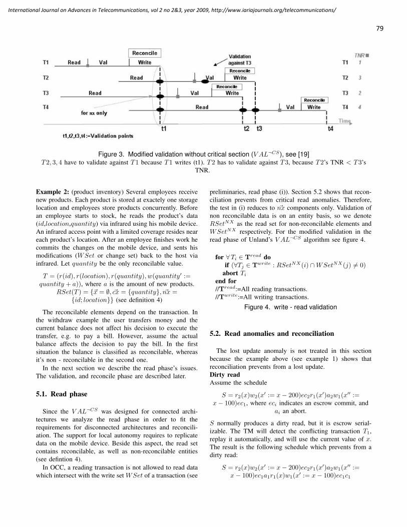
79


Figure 3. Modified validation without critical section (V AL¬CS), see [19]T2, 3, 4 have to validate against T1 because T1 writes (t1). T2 has to validate against T3, because T2’s TNR < T3’s

TNR.

Example 2: (product inventory) Several employees receivenew products. Each product is stored at exactely one storagelocation and employees store products concurrently. Beforean employee starts to stock, he reads the product’s data(id,location,quantity) via infrared using his mobile device.An infrared access point with a limited coverage resides neareach product’s location. After an employee finishes work hecommits the changes on the mobile device, and sents hismodifications (WSet or change set) back to the host viainfrared. Let quantity be the only reconcilable value.

T = (r(id), r(location), r(quantity), w(quantity′ :=quantity + a)), where a is the amount of new products.

RSet(T ) = {~x = ∅, ~cx = {quantity}, ~nx ={id; location}} (see definition 4)

The reconcilable elements depend on the transaction. Inthe withdraw example the user transfers money and thecurrent balance does not affect his decision to execute thetransfer, e.g. to pay a bill. However, assume the actualbalance affects the decision to pay the bill. In the firstsituation the balance is classified as reconcilable, whereasit’s non - reconcilable in the second one.

In the next section we describe the read phase’s issues.The validation, and reconcile phase are described later.

5.1. Read phase

Since the V AL¬CS was designed for connected archi-tectures we analyze the read phase in order to fit therequirements for disconnected architectures and reconcili-ation. The support for local autonomy requires to replicatedata on the mobile device. Beside this aspect, the read setcontains reconcilable, as well as non-reconcilable entities(see defintion 4).

In OCC, a reading transaction is not allowed to read datawhich intersect with the write set WSet of a transaction (see

preliminaries, read phase (i)). Section 5.2 shows that recon-ciliation prevents from critical read anomalies. Therefore,the test in (i) reduces to ~nx components only. Validation ofnon reconcilable data is on an entity basis, so we denoteRSetNX as the read set for non-reconcilable elements andWSetNX respectively. For the modified validation in theread phase of Unland’s V AL¬CS algorithm see figure 4.

for ∀Ti ∈ Tread doif (∀Tj ∈ Twrite : RSetNX(i) ∩WSetNX(j) 6= 0)

abort Tiend for//Tread:=All reading transactions.//Twrite:=All writing transactions.

Figure 4. write - read validation

5.2. Read anomalies and reconciliation

The lost update anomaly is not treated in this sectionbecause the example above (see example 1) shows thatreconciliation prevents from a lost update.Dirty readAssume the schedule

S = r2(x)w2(x′ := x− 200)ec2r1(x′)a2w1(x′′ :=x− 100)ec1, where eci indicates an escrow commit, and

ai an abort.

S normally produces a dirty read, but it is escrow serial-izable. The TM will detect the conflicting transaction T1,replay it automatically, and will use the current value of x.The result is the following schedule which prevents from adirty read:

S = r2(x)w2(x′ := x− 200)ec2r1(x′)a2w1(x′′ :=x− 100)ec1a1r1(x)w1(x′ := x− 100)ec1c1

80


ai indicates an abort by the TM, because a constraint x > 0was violated, and assume x was 200 at r2(x).Non repeatable readAssume the following schedule:

S = r1(x)r2(x)w2(x′ := x + 200)ec2c2r1(x′)ec1c1

As denoted in the schedule x 6= x′.The non repeatable read anomaly is predestinated to brieflysketch out the problem of read anomalies in disconnectedarchitectures. After T1 reads x, x is only present in T1’sworkspace. Each re-read in the workspace will produce thesame result and on the mobile client’s side no non repeatableread is present. But the server side handling is of interest.If the operation is replayed with x’s current value the readis still non-repeatable. Therefore only to lock x, or restrictrepeatable read to workspace level is possible. But, the pointis that the ec-model exploits a non-repeatable read for xvalues to replay the operation. Thus, the ec-model doesn’tsupport an isolation of repeatable read.Phantom readAssume the following schedule:

S = cnt11 := count1(X)insert2(x)ec2c2cnt12 :=count1(X)ec1c1

Both count(X) operations execute in the transaction’sworkspace (mobile client), and they have to produce thesame result, unless a concurrent transaction accesses thesame workspace (not provided by ec), or an explicit re -read was performed. If the count operation is able to getreconciled and a phantom read should be prevented, T1

has to be ec-aborted and replayed with the current state.The result is the following schedule which prevents from aphantom read:

S = cnt11 := count1(X)insert2(x)ec2c2ec1a1cnt11 :=count1(X ′)c1

Summarizing, escrow serializability prevents reconcilablevalues from lost update, dirty read, but phantom read ispossible.

5.3. Validation - and reconcile phase

Validation starts with an escrow commit and the associ-ated change set. As described in the phase validate (ii), eachtransaction starting validation has to validate its change setagainst each (currently) validating transaction with a lowerTNR (see figure 6).

Applying this test to transaction

Tw = (r(id), r(location), r(quantity), w(quantity))

(see example 2) means to test if ~nx = (id, location) or~x = (quantity) intersects with another transaction’s WSetwith a lower TNR. If validation succeeds the modificationsare written, and if either id, location or quantity intersects

with another transaction’s WSet the transaction aborts.But, considering that quantity is a reconcilable value anintersection of quantity does not lead to a unresolvableconflict provided no constraint is violated. According tothat, the test in (ii) is customized to fit the requirementsfor reconcilable elements (see figure 6).

There are some other conclusions. For the validation ofreconcilable elements it’s sufficient to validate the constraintonly (on a value basis). If no constraint is present, validationis unnecessary and the algorithm is directly entering thereconciliation phase, because to reconcile means just toreplay the conflicting operation with the current value.Therefore, only non reconcilable entities enter the validationand write phase, whereas constrained reconcilable elementsneed validation and reconciliation. And in contrast, recon-cilable elements enter the reconcile phase only. Recall, thatreconcile includes to write data.

Assume the validation of location fails. Under this cir-cumstance the transaction aborts due to atomicity, and toprevent from unnecessary reconciliation a validation orderfrom non-reconcile to reconcile ~nx

order→ ~x has to befollowed.

Following this order, to replay means that the operationwhich leads to a conflict is replayed only, because each writeof a non-reconcilable element was still performed, and to re-write again is unwanted due to performance reasons. Thus,the ec-model treats with transaction splitting, because foreach element of ~x a new nested sub transaction is createdand executed by the TM.Conclusions:• (1) A validation order from non-reconcilable to recon-

cilable prevents from unnecessary reconciliation. De-noted by ~nx

order→ ~x• (2) A replay will only replay the conflicting operations.• (3) The replay of an operation leads to a new nested

transaction.

Figure 5 defines the possible states and transitions of theserver phase.

Each non-reconcilable element nxi validates first (1). Ifvalidation succeeds the value of nxi is written (2) andcommitted. If validation fails, T is aborted (3).If each nxi was written successfully each cxi is validatednext (1). The transaction aborts if a constraint is violated (3).Provided a constraint is not violated cxi enters reconciliation(4). In case each nx and cx commits, each xi directly entersthe reconcile phase (5). After the reconciliation and writephase a commit is only possible, since we assume a reliableand physical error free hardware (6). If hardware fails, thisis a matter of recovery. Transactions, like the proposedQuota, try to prevent from constraint violation through pre-estimation. For such transactions a relaxed validation mightbe applicable. It could be indicated by a role, and classifiedby failure probabilities.

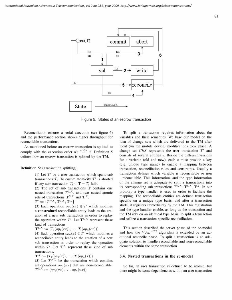
81


Figure 5. States of an escrow transaction

Reconciliation ensures a serial execution (see figure 6)and the performance section shows higher throughput forreconcilable transactions.

As mentioned before an escrow transaction is splitted tocomply with the execution order ~nx

order→ ~x. Definition 5defines how an escrow transaction is splitted by the TM.

Definition 5: (Transaction splitting)

(1) Let T ′ be a user transaction which spans subtransactions Ti. To ensure atomicity T ′ is abortedif any sub transaction Ti ∈ T = Ti fails.(2) The set of sub transactions T contains onenested transaction TNX , and two nested atomicsets of transactions TCX and TX .T ′ := {TNX ,TCX ,TX}(3) Each operation opn(cx) ∈ T ′ which modifiesa constrained reconcilable entity leads to the cre-ation of a new sub transaction in order to replaythe operation within T ′. Let TCX represent thesekind of transactions.TCX := (T1(op1(cx)), . . . , Ti(opn(cx)))(4) Each operation opn(x) ∈ T ′ which modifies areconcilable entity leads to the creation of a newsub transaction in order to replay the operationwithin T ′. Let TX represent these kind of subtransactions.TX := (T1(op1(x)), . . . , Ti(opn(x)))(5) Let TNX be the transaction which containsall operations opn(nx) that are non-reconcilable.TNX := (op1(nx), . . . , opn(nx))

To split a transaction requires information about thevariables and their semantics. We base our model on theidea of change sets which are delivered to the TM afterlocal (on the mobile device) modifications took place. Achange set ChS represents the user transaction T ′ andconsists of several entities e. Beside the different versionsfor a variable (old and new), each e must provide a key(e.g. unique type name) to enable a mapping betweentransaction, reconciliation rules and constraints. Usually atransaction defines which variable is reconcilable or non- reconcilable. This information, and the type informationof the change set is adequate to split a transactions intoits corresponding sub transactions TNX ,TCX ,TX . In ourprototyp a type handler is used in order to faciliate themapping. The reconcilable entities are defined transactionspecific on a unique type basis, and after a transactionstarts, it registers immediately by the TM. This registrationand the type handler enable, as long as the transaction andthe TM rely on an identical type basis, to split a transactionand utilize a transaction specific reconciliation.

This section described the server phase of the ec-modeland how the V AL¬CS algorithm is extended by an ad-ditional reconcile phase. To split a transaction is an ade-quate solution to handle reconcilable and non-reconcilableelements within the same transaction.

5.4. Nested transactions in the ec-model

So far, an user transaction is defined to be atomic, butthere might be some dependencies within an user transaction

82


which allow to weaken the execution order. To obtain aweakened execution order we classify sub transactions ac-cording to the open nested transaction model first (see [29],[12], [30]). Generally, the nested transaction model allowsto relax atomicity and isolation which is often required inmobile, transactional workflow scenarios, or other so calledAdvanced Transaction Models (ATM) (see [31]). In the opennested transaction model a sub transaction, or child, is:

1) open (iso = false), if the results are published toall transactions. It is closed (iso = true), if resultsare published to the parent transaction only (ISOLA-TION).

2) It is vital (vit = true), if to abort leads its parent toabort, too. And, non- vital (vit = false), if an abortdoes not affect its parent (Atomicity, abort

−−→TcTp).

3) T depends on its parent (dep = true), if the parentsabort leads T to abort, too; independent (dep = false)if not (Atomicity, abort

−−→TpTc).

By definition 5 T ′ has to be atomic, thus each T ∈ T ′

is dependent, vital, and closed in order to avoid cascadingrollback (see section 2). For independent, non-vital and openchildren however, it’s possible to change the execution order,and to execute this new class of transactions seperately (pos-sibly pooled or even delayed). E.g. in example 2 assume anadditional transaction which monitors the time an employeeneeds to complete an order. A time variable is incrementedlocally and synchronized at the location with the time of allemployees in order to calculate the average delivery time forthat product. This is an example for an independent, non -vital and open transaction on a reconcilable value.

The drawback of intra transaction dependencies is thatthe TM needs to know them. Our implementation (see 6)as well as our model requires a change set reflecting localmodifications. If the change set provides the informationneeded to classify a transaction a new execution order isapplicable. Based on the classifications for sub transactionsdefinition 6 extends definition 5.

Definition 6: (ec-independency)(1) Let TIN be the set of all independent, non-vital, and open transactions.(2) T ′ is defined as an user transaction with onenested transaction TNX , two nested atomic sets oftransactions TCX and TX , and one atomic, andec-independent set of sub transactions TIN . EachT ∈ TIN is ec-independent.T ′ := {(TNX ,TCX ,TX),TIN}(3) A transaction Tc is ec-independent if the de-pendency function dep of Tc is known for allother transactions Ti ∈ T ′ : Ti 6= Tc, and foreach Ti ∈ T ′ dep validates to true, whereas trueindicates the ec-independency of Tc.(4) ec-independency:iso = 0 ∧ vit = 0 ∧ dep = 0

Although mobile transaction models deal with (non-)substitutable, compensable, temporal, and spatial transac-tions1, none of them have been considered here. Such intratransaction dependencies often originate from the use case’ssemantics and less from the value’s or operation’s semantics.In an interaction scenario (e.g. workflow based) the stateand transition model is able to provide the informationabout such intra dependencies. In mobile computing, serviceselection and composition is context aware and an (formal)interaction model might not given. Hahn’s model [33] ex-ploits transactional properties (non-functional) defined in theinterface to determine which workflow pattern (XOR, AND,and SEQUENCE) is proper for a service interaction.

Our focus is to exploit the semantics on a data andoperations level first, and not to exploit the semantics ofcomplex interaction scenarios. The ec-model may provide areliable foundation other transaction models could rest upon.To benefit from both kinds of semantics (data & value andinteraction) seems to be a worthwhile objective.

6. Example Implementation of the ec Modelwith SDO

Service Data Objects (SDO [34], [35]) are a platformneutral specification and disconnected programming model,which enables dynamic creation, access, introspection, andmanipulation of business objects.

Our implementation (see Lessner [36]) of the transactionmanager (TM) uses SDO graphs and resides between thedata access service (DAS) and the client. This way, the TMfits well into SDO’s vision of being independent of the datasource.

A snapshot of each delivered graph is taken by the TM andeach SDO graph associates a change summary that complieswith the requirements for optimistic concurrency control(see Section 3). To assert ”escrow serializabilty” (providedby the reconciliation algorithm) an association between atransaction and the semantic of this transaction is needed2.This association results in a classification of the transaction(e.g. ”linear dependent”).

An association between a classification and a verifier (seeFigure 8) enables a semantic transaction level (e.g. quotaverifier, escrow concurrency (EC)).

Assume that we have an incoming transaction (T-Level=EC) with a changed data graph. The transactionhandler delivers the transaction to the verifier. To ensureEC, optimistic concurrency control (OCC) is checked first.If OCC is passed there is no serialization conflict. In caseof a conflict the semantic level concurrency control (T-Level=EC) is invoked. This means, two verifier implemen-

1. Temporal and spatial describe transactions subject to temporal andspatial restrictions, respectively.

2. In heterogeneous environments an additional data object could be usedto describe the semantic of a transaction, SDO uses XML as protocol

83


Figure 7. The transaction manager’s architecture

tations come into play (Step 1, Figure 7) in the executionorder ~nx→ ~x.

Each changed attribute is OCC validated against thesnapshot (Step 2, Figure 7). If an OCC conflict exists andthe attribute associates a known ”dependency function”,then reconciliation is possible and a conflict object is in-stantiated that represents the transaction rewrite (withdrawcorrection). If an OCC conflict occurs for an attribute thatis not corrigible, the transaction has to abort. In a secondstep the EC verifier tries to resolve the conflicts (e.g. toreread the balance from the latest snapshot). If any conflictsexist after the EC verifier has finished (e.g. the withdrawamount would exceed the credit limit), the transaction hasto abort, too. Each time a conflict is eventually resolvablethe modification is sent to the replay manager (Step 3,Figure 7) who handles the snapshot’s modifications and thegraph’s changes (Step 4, Figure 7). Finally all changes arewritten and committed to the database. The database requiresisolation level ”repeatable read” during steps 2 to 4.

The snapshot is data centric, which means that there existsa snapshot version of each delivered data object relatedto a transaction. Therefore the knowledge about the type’s

schema is necessary. To acquire this knowledge we decidedto implement a separate meta schema. Another possibilitywould be, to use the schema provided by the implementationof the SDO Data Access Services (DAS). The first possibilityfits better into a general usage of the TM but causes schemaredundancy. In both cases a type handler module is needed,either for accessing the schema of the SDO DAS or foraccessing the additional schema.

7. Alternative conflict detection using RVV

Another approach (not sketched out in section 6) to detectconflicts at row level is the Row Version Verification (RVV)discipline (see [20]). A version indicates a change of atuple/row and it is incremented each time the row is mod-ified. To detect conflicts the TM reads the current versionand compares the current version with the version read bythe transaction. If the two versions differ the transaction isaborted, otherwise committed. RVV’s advantage is a fastconflict detection at row level (DBMS level), and evenmodifications of non ec - transactions (connected or legacy)are detectable. Concerning the ec-model a more fine grained

84


ensure: set of transactions T = {T1, T2, · · · , Tn}ensure: actual database state Ds, set of constraints C(D)ensure: only committed data in read set RSet(i) of Tiensure: Ti = (opik, i = 1, 2, · · · , ki)ensure: T ′ := {TNX ,TCX ,TX}for ∀ eci ∈ {ec1, ec2, · · · , ecn} received doT-number: TNRi := TNC; TNC + +for ∀Tj ∈ Tval : TNRj < TNRido

// test 1 for NX onlyif(RSetNX(i) ∩WSet(j) 6= 0)

abort T ′

else// test 2 for CX onlyensure: RSet(T ′) ⊆ DS

ensure: serial executionif (∃cx:(c = false) then

abort(T’)else

for ∀Ti(opn(cx)) ∈ TCX

//reconciledo Ti(opn(x))

end forfor ∀Ti(opn(x)) ∈ TX

//reconciledo Ti(opn(x))

end forend ifend if

end forend for

Tval each validating transaction.

Figure 6. V AL¬CS with reconciliation for ec serializabil-ity

Figure 8. Abstract design of the transaction manager

detection of changes is required.Assume the row (tupel) (id, location, quantity, v), where

v is the version. Now, two transactions T1 and T2 updatequantitiy concurrently, where T1 writes first. Thus, theversion is incremented and if T2 tries to write, the TM hasto abort T2. To faciliate the TM to support a reconciliation

the TM (1) has to know the row’s current version vc in orderto compare vc with the version read by the transaction. And,(2) if a conflict is detected the TM must be able to indicatea modification of quantity only; Assumed quantity is rec-oncilable. To detect fine grained modifications if a conflictwas detected, requires to re-read the row with its currentversion and to analyze the row. Analyzing means that theTM has to correlate the changes with the matching tupel’scomponent. If such fine grained modifications are detectablereconciliation is possible. Nevertheless, the drawback of (1)and (2) is that during the phases re-reading of the versionand conflict detection, or in the case of a conflict also thephases re-read the row, analyzing it, and reconciliation, therow has to be consistent.

Now, assume the row above is divided into(id, location, ref q, v) and (quantity, vq), where ref qis a reference on quantity. Now two versions have tobe verified, but vq directly indicates modifications forquantity, and prevents the analysis of the whole row.

Another concern is, if modifications, represented by anatomic change set, belong to several rows with correspond-ing versions. Then version verifiying has to be atomic andeach version has to be compared, or another mechanismis provided (e.g. intent versioning). Furthermore, to enablereconciliation for each modified row the TM has also tore-read each conflicting row.

In general, the main difference is RVV tries to write on thedatabase in order to detect conflicts. Whereas the snapshothandler detects conflicts and ensures ec serializability beforeany data is written (sent) into the DB. The snapshot handler’sdrawback is to ensure a synchronous and consistent state be-tween middleware and DB level. Its advantage is a commonrepresentation for the change set, and the snapshots whichalleviates conflict detection. As mentioned, RVV’s advantageis a fast conflict detection at row level (DBMS level), andeven modifications of non ec - transactions are detectable.The overhead for a fine grained error detection and therequired consistence of a row have to be still analyzed.

Another solution like an event driven one, which triggersan event to notify each participating node of a modificationis also conceivable. Each solution has to break through theobstacle to keep versions or snapshots synchronous acrosslayers and during concurrent access.

In summary, RVV is an easy to understand solution andit’s generally applicable on the ec-model, especially for nxentities. RVV itself is a more architectural aspect which maybe needed in some scenarios. Versioning in principle is awell known discipline.

8. Performance of the ec-model

We ran a series of simulations of concurrent withdrawtransactions accessing the same account. The transactionconfiguration parameters were as following: Reading the

85


Figure 9. Performance of EC compared with OCC and locking

balance took less than 10 ms, the user’s thinking time wasrandomly chosen between 1 and 2 seconds, and the writetime needed about 10 ms. The throughput results for up to30 concurrent transactions is shown in Figure 9.

Running 30 transactions in parallel generated 23 seri-alization conflicts which triggered the replay mechanism.The net processing time for a transaction or a replay wasapproximately 20 ms. The total elapsed time for all 30transactions was t = 2.1 sec which is consistent with theminimum thinking time (1 sec) plus the time for processing30 transactions ((30 + 23) × 20 ms = 1.06 sec) in escrow-serialization mode. The results show that we achieved anelapsed time close to the theoretical limit considering thenumber of replays necessary.

The nearly linear growth of the throughput when usingthe escrow concurrency control indicates that we have notreached the throughput limit. Given a processing time of 20ms, the theoretical limit for this scenario (”hot spot” on thebalance) would reach 50 transactions per second.

In contrast, the traditional OCC and locking schemescould not interleave the transactions and resulted in essen-tially serial processing. Therefore the performance saturatedat 1/1.5 = 0.66 transactions per second, where 1.5 sec arethe average transaction duration.

In order to have a more complex example than thewithdraw transaction we used the popular TPC-C benchmark[37] and analysed the New Order (NOrder-Ta) and the Pay-ment (Pay-Ta) transactions. The NOrder-Ta exhibits two ”hotspots” with linear dependency semantics defined in section4. One is the update of the next order id (d next o id) in thedistrict table and the other is the update of the quantity on

stock (s quantity) for each line item. The Pay-Ta contains”hot spots” in the tables Warehouse, District, and Customer.Again, the semantics of the transaction is linear dependentwith gradient 1 (see section 4) as it deals with updatingthree balances with a fixed amount, updating the year todate payment by the same amount, and incrementing thepayment count.

In total we have identified 7 situations where the escrow-serialization mechanism could be beneficial for performance.First tests indicate a substantial improvement over traditionallocking mechanism.

9. Conclusions

Mobile transactions have special demands for the trans-action management. We propose a transaction model that isnon-blocking and is reconciling conflicting transactions byexploiting the semantic of the transaction. A simple abort-replay mechanism can produce reconciliation in the senseof escrow serializability. The abort-replay algorithm detectsconflicts by rereading the data. The mechanism is easy toimplement and can make use of update operation when read- and write set overlaps.

If all writes are postponed until the commit is issuedand the reread and write operations during reconciliationare executed serialized or serial, then no inconsistent datawill be read. A further option is to use consistent snapshots.Independent from the mechanism the read phase should beexecuted with optimistic concurrency control.

In contrast, the reconciliation phase should run in a pre-claiming locking mode. This ensures efficient sequential

86


processing of competing transactions without delays as userinput is already available and starvation is avoided. Withthis marginal condition the escrow serialization algorithmhas the potential to outperform other mechanisms.

For the class of linear dependent transactions it is suffi-cient for reconciliation to know the client state at begin oftransaction, the state produced by the client transaction onthe client site, and the database server state at commit time.

10. Future work

The following outlines some important points of futureresearch. Even if first simulations show higher transactionthroughput, they need to become re-engineered. More com-plex business scenarios with several devices involved andan implementation based at databases driver level are someaspects. Such an implementation will simplify benchmarksand ease the existing SDO-implementation. Concerning thedevelopment of software, developers should be supportedby methods to define or classify dependency functions fortransactions which intend to use escrow serializability. Ingeneral, to define and detect a transaction’s semantics man-ually is a drawback of many other transaction models usingsemantic properties. Regarding our model, an investigationof the opportunities to derive dependency functions basedon common interaction patterns or on a data type base isintended. A not mentioned, but relevant concern is recoveryin the escrow model, and more research has to be done inthis field.

Acknowledgements

This paper was inspired by discussions with the membersof the DBTech network and the ideas presented during theDBTech Pro workshops. The DBTech Project was supportedby the Leonardo da Vinci programme during the years 2002- 2005.

References

[1] Fritz Laux and Tim Lessner. Transaction processing in mobilecomputing using semantic properties. The First InternationalConference on Advances in Databases, Knowledge, and DataApplications, DBKDA, Cancun, Mexico, 169, March 2009.

[2] J.H. Abawajy and M. Mat deris. Supporting disconnectedoperations in mobile computing. Computer Systems andApplications, ACS/IEEE International Conference on, 0:911–918, 2006.

[3] Shirish Hemant Phatak and Badri Nath. Transaction-centricreconciliation in disconnected client-server databases. Mob.Netw. Appl., 9(5):459–471, 2004.

[4] Joanne Holliday, Divyakant Agrawal, and Amr El Abbadi.Disconnection modes for mobile databases. Wirel. Netw.,8(4):391–402, 2002.

[5] Hector Garcia-Molina. Using semantic knowledge for trans-action processing in a distributed database. ACM Trans.Database Syst., 8(2):186–213, 1983.

[6] Abdel Aziz Farrag and M. Tamer Ozsu. Using semanticknowledge of transactions to increase concurrency. ACMTrans. Database Syst., 14(4):503–525, 1989.

[7] Shi-Ming Huang and Chien-Ming Huang. A semantic-basedtransaction model for active heterogeneous database systems.Systems, Man, and Cybernetics, 3:2854–2859, 1998.

[8] Dimitrios Georgakopoulos, Marek Rusinkiewicz, and Amit P.Sheth. On serializability of multidatabase transactionsthrough forced local conflicts. In Proceedings of the SeventhInternational Conference on Data Engineering, pages 314–323, Washington, DC, USA, 1991. IEEE Computer Society.

[9] Sharad Mehrotra, Rajeev Rastogi, Henry F. Korth, and Abra-ham Silberschatz. Non-serializable executions in heteroge-neous distributed database systems. In PDIS ’91: Proceedingsof the first international conference on Parallel and dis-tributed information systems, pages 245–252, Los Alamitos,CA, USA, 1991. IEEE Computer Society Press.

[10] Shi Ming Huang, Irene Kwan, and Chih He Li. A studyon the management of semantic transaction for efficient dataretrieval. SIGMOD Rec., 31(3):28–33, 2002.

[11] Peter Graham and Ken Barker. Effective optimistic con-currency control in multiversion object bases. In ElisaBertino and Susan Darling Urban, editors, ISOOMS ’94: Pro-ceedings of the International Symposium on Object-OrientedMethodologies and Systems, volume 858 of Lecture Notesin Computer Science, pages 313–328, London, UK, 1994.Springer-Verlag.

[12] Gerhard Weikum and Gottfried Vossen. Transactional infor-mation systems: theory, algorithms, and the practice of con-currency control and recovery. Morgan Kaufmann PublishersInc., San Francisco, CA, USA, 2001.

[13] Fritz Laux, Tim Lessner, and Martti Laiho. Semantic trans-action processing in mobile computing. In Cherif Branki,Brian Cross, Gregorio Daz, Peter Langendrfer, Fritz Laux,Guadalupe Ortiz, Martin Randles, A. Taleb-Bendiab, FrankTeuteberg, Rainer Unland, and Gerhard Wanner, editors,TAMoCo, volume 169 of Frontiers in Artificial Intelligenceand Applications, pages 153–164. IOS Press, 2008.

[14] Qi Lu and M. Satyanaranyanan. Isolation-only transactionsfor mobile computing. Operating Systems Review, 28:81–87,1994.

[15] H. T. Kung and John T. Robinson. On optimistic methods forconcurrency control. ACM Trans. Database Syst., 6(2):213–226, 1981.

[16] Jim Gray, Pat Helland, Patrick O’Neil, and Dennis Shasha.The dangers of replication and a solution. In SIGMOD’96: Proceedings of the 1996 ACM SIGMOD internationalconference on Management of data, pages 173–182, NewYork, NY, USA, 1996. ACM.

87


[17] G. D. Walborn and P. K. Chrysanthis. Supporting semantics-based transaction processing in mobile database applications.In SRDS ’95: Proceedings of the 14TH Symposium on Re-liable Distributed Systems, page 31, Washington, DC, USA,1995. IEEE Computer Society.

[18] Gary D. Walborn and Panos K. Chrysanthis. Transactionprocessing in pro-motion. In SAC ’99: Proceedings of the1999 ACM symposium on Applied computing, pages 389–398,New York, NY, USA, 1999. ACM.

[19] Rainer Unland. Optimistic concurrency control revisited.Technical report, Department of Business Informatics, Uni-versity of Muenster, 1994.

[20] Martti Laiho and Fritz Laux. Data access using rvv disciplineand persistence middleware. e RA - 3, Greece, 2008.

[21] Hector Garcia-Molina, Jeffrey D. Ullman, and JenniferWidom. Database Systems: The Complete Book. PrenticeHall PTR, Upper Saddle River, NJ, USA, 2001.

[22] Abraham Silberschatz, Henry F. Korth, and S. Sudarshan.Database System Concepts, 5th Edition. McGraw-Hill BookCompany, 2006.

[23] K. A. Momin and K. Vidyasankar. Flexible integrationof optimistic and pessimistic concurrency control in mobileenvironments. In Julius Stuller, Jaroslav Pokorny, Bern-hard Thalheim, and Yoshifumi Masunaga, editors, ADBIS-DASFAA ’00: Proceedings of the East-European Conferenceon Advances in Databases and Information Systems HeldJointly with International Conference on Database Systemsfor Advanced Applications, volume 1884 of Lecture Notesin Computer Science, pages 346–353, London, UK, 2000.Springer-Verlag.

[24] Stefano Ceri and Susan S. Owicki. On the use of optimisticmethods for concurrency control in distributed databases. InBerkeley Workshop, pages 117–129, 1982.

[25] Ho-Jin Choi and Byeong-Soo Jeong. A timestamp-based op-timistic concurrency control for handling mobile transactions.In Marina L. Gavrilova et al., editor, ICCSA (2), volume3981 of Lecture Notes in Computer Science, pages 796–805.Springer, 2006.

[26] Adeniyi A. Akintola, G. Adesola Aderounmu, A. U. Osakwe,and Michael O. Adigun. Performance modeling of an en-hanced optimistic locking architecture for concurrency controlin a distributed database system. Journal of Research andPractice in Information Technology, 37(4), 2005.

[27] V. Krishnaswamy, D. Agrawal, J. L. Bruno, and A. ElAbbadi. Relative serializability: An approach for relaxingthe atomicity of transactions. SIGMOD/PODS 94, 1994.

[28] Klaus R. Dittrich and Stella et al. Gatziu, editors. AktiveDatenbanksysteme. dpunkt Verlag, Heidelberg, BW, GER,2000.

[29] J. E.B. Moss. Nested transactions: an approach to reliabledistributed computing. Massachusetts Institute of Technology,Cambridge, MA, USA, 1985.

[30] Kyong-I Ku and Yoo-Sung Kim. Moflex transaction model formobile heterogeneous multidatabase systems. In RIDE ’00:Proceedings of the 10th International Workshop on ResearchIssues in Data Engineering, page 39, Washington, DC, USA,2000. IEEE Computer Society.

[31] Sushil Jajodia and Larry Kerschberg, editors. AdvancedTransaction Models and Architectures. Kluwer, 1997.

[32] Jim Gray and Andreas Reuter. Transaction Processing:Concepts and Techniques. Morgan Kaufmann, 1993.

[33] Katharina Hahn and Heinz Schweppe. Exploring transactionalservice properties for mobile service composition. In MarkusBick, Martin Breunig, and Hagen Hopfner, editors, MMS,volume 146 of LNI, pages 39–52. GI, 2009.

[34] M. Adams and C. Andrei et al. Service data objects for javaspecification. OSOA (BEA Systems, IBM, et al.), 2.1, 2006.

[35] J. Beatty, S. Brodsky, M. Nally, and R. Patel. Next-generationdata programming. BEA Systems, IBM, 2003.

[36] Tim Lessner. Transaktionsverarbeitung in disconnected Ar-chitekturen am Beispiel von Service Data Objects (SDO)und prototypische Implementierung eines Transaktionsframe-works. Diploma thesis (ger), 2007.

[37] TPC. Tpc benchmark c, standard specification, revision 5.9,2007.

88


A FAMILY OF RECURSIVE LEAST-SQUARES ADAPTIVE ALGORITHMS SUITABLE FOR FIXED-POINT IMPLEMENTATION

Constantin Paleologu, Silviu Ciochină, and Andrei Alexandru Enescu

Telecommunications Department, University Politehnica of Bucharest, Romania

e-mail: {pale, silviu, aenescu}@comm.pub.ro

ABSTRACT

The main feature of the least-squares adaptive algorithms is their high convergence rate. Unfortunately, they encounter numerical problems in finite precision implementation and especially in fixed-point arithmetic. The objective of this paper is twofold. First, an analysis of the finite precision effects of the recursive least-squares (RLS) algorithm is performed, outlining some specific problems that could appear in fixed-point implementation; consequently, we present a modified version of the RLS algorithm suitable for fixed-point implementation, using an asymptotically unbiased estimator for the algorithm’s cost. Second, we extend the procedure for the case of QR-decomposition-based least-squares lattice (QRD-LSL) adaptive algorithm, a “fast” member of RLS family, with good numerical properties. The reduced dynamics of the algorithm’s parameters leads to facility for fixed-point implementation. The simulations performed on a fixed-point digital signal processor (DSP) sustain the theoretical findings. Also, as a practical aspect of this work, we illustrate the performance of the proposed QRD-LSL algorithm for noise reduction.

Index Terms— Adaptive filters, fixed-point implementation, noise reduction, QR-decomposition-based least-squares lattice (QRD-LSL) algorithm, recursive least-square (RLS) algorithm.

1. INTRODUCTION The Recursive Least Squares (RLS) algorithm is one of the most popular adaptive algorithms, mainly due to its fast convergence rate [1]. Nevertheless, there are some major drawbacks related to the high computational complexity and the large dynamic range of the algorithm’s variables. The first issue could be overcome by using a fast RLS algorithm, in the meaning that the computational cost increases linearly with the number of adjustable parameters. The last drawback is more severe and could cause unwanted effects in a fixed-point arithmetic context,

such as overflow or stalling phenomena [2]. In this paper we focus on some numerical problems of the RLS algorithm and present a modified version of this algorithm, which is more suitable for fixed-point implementation. For practical reasons, the proposed procedure is applied to the QR-decomposition-based least-squares lattice (QRD-LSL) algorithm, which is a fast member of the RLS family with robust numerical behavior.

The QRD-LSL algorithm [3] combines the good numerical properties of QR-decomposition and the desirable features of a recursive least-squares lattice. Whereas the recursive QR-decomposition-based recursive least-squares (QRD-RLS) algorithm [1] requires a high computational load on the order of L2 (where L is the filter order), in terms of both the number of processing cells and the computation per iteration, the QRD-LSL implementation is fast in the sense that these numbers are reduced to a linear dependence on L. This algorithm exploits the shifting property of serialized input data (the Toeplitz structure of the data matrix) to perform joint-process estimation in a fast manner. By virtue of this facts, the QRD-LSL algorithm is endowed with a highly desirable set of operational and implementation characteristics such as good numerical properties (inherited from QR-decomposition), good convergence properties (due to the RLS nature), and a high level of computational efficiency (resulted from the modular, lattice-like structure). The combination of these characteristics makes the QRD-LSL a powerful adaptive algorithm, suitable for a wide range of applications, e.g., echo cancellation, interference rejection, or noise reduction [4]–[10].

Another implication of the modular structure of the QRD-LSL algorithm is that it lends itself to the use of very large-scale integration (VLSI) technology for its hardware implementation. Of course, the use of this sophisticated technology can be justified only if the application of interest calls for the use of VLSI chips in large number. Otherwise, a digital signal processor (DSP) implementation represents a proper solution. In this case, an important practical aspect is related to the dynamic range of the algorithm’s parameters. It is known that in two-complement fixed-point implementation context the

This work was supported by the UEFISCSU Romania under Grants PN-II-“Idei” no. 65/01.10.2007 and no. 331/01.10.2007.

89


absolute values of all involved parameters have to be smaller than 1. In the case of the classical QRD-LSL algorithm the cost functions asymptotically increase; theoretically, they are upper bounded by 1/ (1 )λ− , where λ is the exponential weighting factor ( 0 1λ< ≤ ) [1]. When dealing with a value of λ very close to 1 (which is the case in most of the applications due to stability reasons [11]), very large values of the cost functions are expected. In order to prevent any unwanted overflow phenomenon it is necessary to scale the cost function. As a consequence, the major drawback is the precision loss because of these factors.

In the first part of this work we analyze the behavior of the RLS algorithm in fixed-point arithmetic, revealing some specific problems that could appear in this context. In order to overcome these potential issues we present a modified version of the RLS algorithm that is suitable for fixed-point implementation. The main idea is to use an asymptotically unbiased estimator for the algorithm’s cost function, in order to reduce the dynamic range of this parameter. The idea can be applied to other RLS-based algorithms. In this paper we extend the procedure for the case of QRD-LSL algorithm. Consequently, a modified version of this algorithm is obtained. The reduced dynamic of the parameters leads to facilities for fixed-point implementation.

The paper is organized as follows. Section 2 contains certain backgrounds of the classical RLS algorithm, outlining several specific problems that could appear in fixed-point implementation. In Section 3 we establish a connection between the dynamic range of variables and the initial convergence rate, and we present a modified version of the RLS algorithm suitable for fixed-point implementation. The modified version of the QRD-LSL algorithm is developed in Section 4. The simulation results are presented in Section 5. A summarized discussion of the main results is given in Section 6. Finally, Section 7 briefly concludes this work.

2. RLS ALGORITHM BACKGROUND AND

ANALYSIS

The well-known RLS adaptive algorithm [1] uses a cost function defined as an estimate of the mean square-error, i.e.,

( ) ( ) ( ) ( )2 2

11

nn i

iJ n e i J n eλ λ−

== = − +∑ n

1

, (1)

where 0 λ< ≤ is the exponential weighting factor and e(i) is the difference between the desired response d(i) and the output y(i) produced by an adaptive transversal filter. That is,

( ) ( ) ( ) ( ) ( ) ( )He i d i y i d i n i= − = −w x , (2) where x(i) is the tap-input vector at time i and w(n) is the tap-weight vector at time n. The superscript H denotes Hermitian transposition (transposition and complex conjugation).

This estimate of the cost function induces similar estimates for the correlation matrix Φ(n) and the cross-correlation vector θ(n), i.e.,

, (3) ( ) ( ) ( ) ( ) ( ) ( )1

1n

n i H H

in i i n nλ λ−

== = − +∑Φ x x Φ x x n

n

, (4) ( ) ( ) ( ) ( ) ( ) ( )* *

11

nn i

in i d i n n dλ λ−

== = − +∑θ x θ x

where superscript * denotes complex conjugation. The optimum value of the tap-weight vector w(n), for which the cost function J(n) from (1) attains its minimum value is defined by the normal equation written in matrix form:

( ) ( ) (n n n=Φ w θ ) . (5) The regular procedure is to apply the matrix inversion lemma in (3) in order to solve (5). Denoting

( ) ( )1n n−=P Φ (6) and defining the Kalman vector

( ) ( ) ( )( ) ( ) ( )

1111 1H

n nn

n n nλλ

−= ⋅

+ −

P xk

x P x (7)

the inverse of the estimate of the correlation matrix is computed in a recursive manner as [1]

( ) ( ) ( ) ( ) ( )1 11 1Hn n n n nλ λ

= − − −P P k x P . (8)

Finally, the recursive equation for updating the tap-weight vector is ( ) ( ) ( ) ( )*1n n n α= − +w w k n , (9) where α(n) is the a priori estimation error defined by ( ) ( ) ( ) ( )1Hn d n n nα = − −w x (10) The initial value of P(n) is chosen

90


( ) 10 δ −=P I , (11) where δ is the regularization parameter (a positive constant) and I is the identity matrix. This initial value assures the non-singularity of the correlation matrix Φ(n). In the case of a stationary environment or a slowly time-varying one, the parameter δ should be assigned a small value for high signal-to-noise ratio (SNR) and a large value for low SNR [12].

Next, in order to analyze the behavior of the RLS algorithm in finite precision implementation, let us examine some of its main parameters. Following (1) and (3), the expectations of the cost function J(n) and of the matrix Φ(n) are

( ){ } ( ){ }211

n

E J n E e nλλ

−≅

−, (12)

( ){ } 11

n

E n λλ

−≅

−Φ R , (13)

where R is the correlation matrix of input data. It can be noticed that J(n) is a biased estimate of E{|e(n)|2} and similarly Φ(n) is a biased estimate of R, i.e.,

( ){ } ( ){ 211n

E J n E e nλ→∞

≅− } , (14)

( ){ } 11n

E nλ→∞

≅−

Φ R . (15)

Some classes of applications, e.g., [6], [7] require a

high memory algorithm, which means that the value of the exponential weighting factor λ is very close to 1. In this case very large values for the parameters from (14) and (15) could result, causing unwanted finite precision effects in a practical implementation. Apparently, the RLS algorithm avoids this problem by using the inverse of the matrix Φ(n). Therefore, the maximum values of the elements of the matrix P(n) result in the initialization phase of the algorithm, according to (11). Nevertheless, the “reverse” problem persists because the values of the elements of the matrix P(n) decrease towards very small values close to zero, when λ is close to 1.

For example let us consider the following scenario. The fixed point two’s complement arithmetic with a word length of B + 1 bits is used and the input signal is a white Gaussian noise, so that R = σx

2I, where σx2 is the input

signal variance. We assume the input signal power upper bounded, so that

, (16) 2

x aσ ≤

where a is a positive constant. In addition, for the RLS algorithm to work, a persistent excitation condition [13] must be imposed, i.e., , (17) 2

x bσ ≥ where b is a positive constant. Following (13) results

( )2

1x

nn

σλ→∞

=−

Φ I , (18)

( ) 2

1n

x

n λσ→∞

−=P I . (19)

Consequently, the elements of the main diagonal of P(n), denoted here by P(i,i)(n), are asymptotically bounded by

( ) ( ),1 1

i i na bλ λ− −≤ ≤P . (20)

On the other hand, according to (11), it results that

( ) ( ),10i i δ

=P . (21)

Therefore, a scaling procedure is required to avoid overflow phenomenon. The scaling factor 0 < s < 1 has to be chosen such that , (22) 1sM < where

1 1max ,Mbλ

δ−⎧ ⎫= ⎨ ⎬

⎩ ⎭. (23)

Nevertheless, reducing the values of the elements of P(n) by scaling may lead to a stalling phenomenon. This phenomenon appears when P(n) becomes a zeros matrix, so that, according to (8), the RLS algorithm is “frozen”. To avoid this situation it is necessary that

1 2 Bsaλ −−> . (24)

Consequently,

21

Ba s 1Mλ

−⋅< <

− (25)

91


and that implies

21

B aMλ

>−

. (26)

In (23) the case (1 – λ)/b > 1/δ is improbable for a value of λ very close to 1, so that usually M = 1/δ and the algorithm is not sensitive to decrease of excitation.

3. MODIFIED RLS COST FUNCTION

Taking into account the previous discussion it would be very helpful to use an unbiased estimator of the matrix Φ(n). For this reason, the cost function from (1) can be modified as follows [14]:

( ) ( ) ( ) ( ) ( ) ( )2 2

11 1

nn i

i1J n e i J nλ λ λ λ−

== − = − + −∑ e n .

(27) In this case

( ){ } ( ) ( ){ }21 nE J n E e nλ≅ − (28)

is an asymptotically unbiased estimator of the mean square-error.

Following this idea we have to perform the same modification in (3) and (4) obtaining

( ) ( ) ( ) ( )

( ) ( ) ( ) (1

1

1 1

nn i H

i

H

n i i

n n

λ λ

λ λ

−

== − =

= − + −

∑Φ x x

Φ x x )n (29)

( ) ( ) ( ) ( )

( ) ( ) ( ) ( )

*

1

*

1

1 1

nn i

in i d i

n n

λ λ

λ λ

−

== − =

= − + −

∑θ x

θ x d n (30)

According, ( ){ } ( )1 nE n λ≅ −Φ R (31)

is an asymptotically unbiased estimator of the correlation matrix.

As a consequence of these modifications, the Kalman vector from (7) has to be evaluated as [14]

( ) ( ) ( )( ) ( ) ( )

1

11

H

n nn

n n nλλ

−=

+ −−

P xk

x P x, (32)

where ( )nP is the inverse of the matrix ( )nΦ . The others algorithm’s relations remain the same [i.e., equations (8), (9), and (10)].

Next, let us perform a brief convergence analysis of this modified RLS algorithm. First we assume that the desired response d(i) and the tap-input vector x(i) [see (2)] are related by the linear regression model

( ) ( )0 0

Hd i i e i= +w x ( ) , (33) where w0 is the regression parameter vector of the model and e0(i) is the measurement noise, assumed to be white with zero mean and variance σ0

2, and independent of x(i). As a result of the initialization procedure, (29) becomes

( ) ( )0nn λ δ= +Φ I Φ n , (34)

where ( )0 nΦ is a particular solution, i.e.,

( ) ( ) ( ) ( )01

1n

n i H

in λ λ −

== − ∑Φ x xi i

)i

⎫⎬ 0

. (35)

Using (34), (35), (33), and (30) in (5) we get

( ) ( ) ( ) ( ) ( )

( ) ( ) ( ) ( ) ( ) (1

*0 0

1 1

1

1 1

nn i H n

in n

n i H n i

i i

i i n n

i i i e

λ λ λ δ

λ λ λ λ

−

=

− −

= =

− + =

= − + −

∑

∑ ∑

x x w w

x x w x

(36) Taking the expectation of both sides of (36) and taking into account that

( ) ( )*0

1

nn i

iE i e iλ −

=

⎧ =⎨⎩ ⎭∑ x , (37)

( ) ( )1 1

nn i H

iE i iλ

λ−

=

⎧ ⎫ =⎨ ⎬−⎩ ⎭

∑Rx x , (38)

we obtain ( ) ( ){ } 0

n E nλ δ+R I w R= w . (39) Therefore,

( ){ } 0nE n

→∞=w w (40)

so that w(n) is an asymptotically unbiased estimator of w0. The initial convergence rate of the modified algorithm depends on how “fast” the product λnδ decreases to zero.

92


Performing the same analysis for the classical RLS algorithm we get

. (41) ( )( ) ( ){ } 01 n E nλ λ δ+ − =R I w Rw

Comparing (39) to (41) it is obvious that the classical RLS algorithm has a faster initial convergence rate than the modified algorithm for the same λ and δ. Anyway, if we use for the classical RLS algorithm a value of the regularization parameter equal to δ and for the modified algorithm the value ( )' 1δ δ λ= − (42) both RLS algorithms achieve the same initial convergence rate.

Finally, let us analyze the dynamic range of the elements of the matrix ( )nP . In a similar manner as in the case of the classical RLS algorithm we find

1 1' max ,'

Mbδ

⎧ ⎫= ⎨ ⎬⎩ ⎭

, (43)

12'

B a sM

− < < , (44)

so that . (45) 2 'B aM> For 'δ δ= , the probability of stalling phenomenon becomes significantly lower. Nevertheless, if 'M is chosen as ' 1/ 'M δ= , the probability of overflow due to small signal becomes higher.

It can be concluded that the fast initial convergence rate, being dependent on δ, is conditioned by the numerical resolution. Even in the modified version, the estimate of the mean square error is biased at the beginning of the process and similar property results for the matrix ( )nΦ . In addition, the initial value P(0) from (11) is an arbitrary starting point, without any relation with the input signal, but important for the initial convergence rate. We propose a more natural way for initialization of the cost function, suggested by the well-known averaging algorithm

( )( ) ( )

( ) ( )

2

2

1 11 , 1

1 11 ,

n J n e n nn nJ n

N

N

J n e n nN N

−⎧ − + ≤ ≤⎪⎪= ⎨ −⎪ − + >⎪⎩

N (46)

In the first N steps, ( )J n is the sample mean of |e(n)|2, i.e.,

( ) ( ) 2

1

1 n

iJ n e i

n == ∑ (47)

Alternatively, the above cost function can be written as ( ) ( ) ( ) ( )( ) ( ) 2

λ 1 1 λJ n n J n n e n= − + − (48) where

( )1 1for 1

1λ1for

1

n nnn

n

λ

λλ

−⎧ < ≤⎪⎪ −= ⎨⎪ >⎪ −⎩

(49)

For n = 1, λ(1) = 0 is not acceptable so that the iterations start from n = 2, considering the initial value ( ) ( ) 21 0x −=P I (50)

In order to agree assumption (17) the algorithm starts only when x(0) > b. The initial convergence rate depends on the starting value x2(0) but this dependence is considerably reduced because of the low memory behavior (i.e., small λ) in the initial part of the process. The main advantage of the algorithm consists of the fact that ( )nΦ is an unbiased estimator of R, almost every time.

4. QRD-LSL ALGORITHMS WITH REDUCED

DYNAMICS OF PARAMETERS The classical RLS is not very frequently used in practical application mainly due to its high computational complexity (on the order of L2). For this reason, the fast RLS algorithms are preferred in practice (e.g., [15]). Among these, the QRD-LSL algorithm represents one of the most attractive choices, mainly due to its robust numerical features [9].

In order to extend the idea of the modified cost function from Section 3 to the case of the QRD-LSL algorithm, let us consider the time series ( ) ( ) ( )1 , 2 , ,x x x… n (i.e., the input signal) that occupies the

time interval 1 i n≤ ≤ , assuming that ( ) 0x i = for 0i ≤ . Most of the notations from [1] will be involved in the following development. The data matrix used in a least-squares estimation problem can be expressed as

*

1 , 1 1 , 1* *

1

(1) 0 0( ) ( 1) ( 2) ( 2)

( ) ( 1) ( )

m f m m b mHm

xn n n n

x n n x n m

+ − − −

−

⎡ ⎤⎢ ⎥⎢ ⎥= − − −⎢ ⎥⎢ ⎥− −⎣ ⎦

A d A d

x

, (51)

93


where subscript m = 1, 2,…, L is the prediction order and 1( 2)b

mJ n−

*

* *1

* * *

(1) 0 0

(2) (1) 0( 2)

( 2) ( 1) ( )

m

x

x xn

x n x n x n m

−

⎡ ⎤⎥⎥⎥

⎥⎦

⎢⎢

− = ⎢⎢ ⎥⎢ − − −⎣

A

,

) )

⎤⎥

, (52)

[ ]1( 1) ( 1), , ( 1) Tm n x n x n m− − = − − +x … (53)

* *

, 1( 1) (2), , ( 1) ,T

f m n x x n−⎡ ⎤− = −⎣ ⎦d … (54)

*

, 1( 2) 0, , ( 1)T

b m n x n m−⎡ ⎤− = − −⎣ ⎦d … . (55)

where superscript T denotes transposition. Let us denote by

an n-by-n unitary matrix and by an -by- upper triangular matrix. The

exponential weighting matrix from the classical QR-decomposition is

( )m nQ ( )m nR( 1m + ( 1m +

(56) { }1 2 ( 1)( ) diag , , ,1

1cn n

c T

nn

λλ λ− − −⎡

= = ⎢⎢ ⎥⎣ ⎦

Λ 0Λ

0…

In order to approach the cost function from (27), a

modified form of the previous matrix will be used in our development, i.e.,

{ }1 2 ( 1)( ) (1 )diag , , ,1

1n n

T

nn

λλ λ λ

λ− − −⎡ ⎤

= − = ⎢ ⎥−⎢ ⎥⎣ ⎦

Λ 0Λ

0… .

(57) Using (57) and following the QR-decomposition we have:

1/22 1

1/2 ( 1)/2 *

1/2 1/2 1/2, 2 2 , 2

1/2 1/2, 2 , 21/2 * 1/2 1/2 *

1

1 0( 2) ( ) ( )

0 1

(1 ) (1) 0

( 1) ( 2) ( 2)

( 1) ( 2)

(1 ) ( ) (1 ) ( 1) (1 ) ( )

T

m mT

n T

f m m b m

f m b mHm

n n n

x

n n

n

n

n

x n n x n

λ λ

λ λ λ

λ λ

λ λ λ

− +

−

− − −

−

−

⎡ ⎤⎢ ⎥

−⎢ ⎥⎢ ⎥⎢ ⎥⎣ ⎦

⎡ ⎤−⎢⎢ − − −⎢=⎢ −⎢⎢ − − − − −⎣ ⎦

00 Q 0 Λ A

0

0

p R p

v 0 v

x m

− −

⎥⎥⎥⎥⎥⎥

(58) Let B(n) denote the matrix on the right-hand term of (58). We use a unitary matrix to annihilate the vector

, except for its first element, denoted by ( 2n −P

. A new element is generated, namely, −

, 1( 1)f m nπ − − , in the first column. Next, we use the unitary

matrix 2 ( 1)m n− −T to update the vectors , 2 ( 1)f m n− −p ,

, 2 ( 2b m n− )−p , and the matrix 2 ( 2m n− )−R . Angle-normalized forward and delayed backward prediction errors, , 1( )f m nε − and , 1( 1)b m nε − − , are generated in complex conjugate forms and all the elements of the vector

1( 1)Hm n− −x are annihilated, i.e.,

2

1/2 ( 1)/2 *

, 2 2 , 2

1/2 1/2, 1 1

1/2, 1

1/2 * 1/2 *, 1 , 1

( 2)1 ( )( 1) 1

(1 ) (1) 0( ) ( 1) ( 1)

( 1) ( 2)

( 1)

(1 ) ( ) (1 ) ( 1)

T

Tm

n T

f m m b m

T bf m m

f mT

f m b m

nn

n

xn n n

n J

n

n n

λ λ

λ π λ

λ

λ ε λ ε

−

−

− − −

− −

−

− −

−⎡ ⎤ ⎡ ⎤⋅ ⋅⎢ ⎥ ⎢ ⎥

− ⎢ ⎥⎢ ⎥ ⎣ ⎦⎣ ⎦

n

⎡ ⎤−⎢ ⎥

− −⎢⎢⎢ − −=⎢⎢ −⎢⎢ − − −⎣ ⎦

P 00 B0 T 0

0p R p

0

v 0 0

0

⎥⎥⎥⎥⎥⎥⎥

(59) Let C(n) denote the matrix on the right-hand term of (59). We can write:

1*

, 1 , 1

1

, 1 , 1

1/2 ( 1)/2 *

, 2 2 , 2

, 1 11/2

, 1

1 0 0

( )0 ( 1) ( 1)

0 ( 1) ( 1

(1 ) (1) 0( ) ( 1) ( 1)

( ) ( 1)

( 1)

(1 )

T T

mT T

b m b m

n mT T

b m b m

n T

f m m b m

T bf m m

f m

nc n s n

s n c n

xn n

n J

n

λ λ

π

λ

λ

−

− −

− −

− −

−

− − −

− −

−

⎡ ⎤⎢ ⎥⎢ ⎥⎢ ⎥

− −⎢ ⎥⎢ ⎥⎢ ⎥⎢ ⎥− − −⎣ ⎦

−− −

−=

−

−

0 00 I 0 0 0

C0 00 0 0 I 0

0 0

0p R p

0

v 01/2 *

, ( ) 0Tf m nε

)

n

n

0

⎡ ⎤⎢ ⎥⎢ ⎥⎢ ⎥⎢ ⎥⎢ ⎥⎢ ⎥⎢ ⎥⎢ ⎥⎣ ⎦0

(60) where I denotes identity matrices. Furthermore, the following updates result:

1/21

, 11

( 2)( 1)

( 1)

bm

b m bm

J nc n

J n

λ −−

−

−− =

−, (61)

)), 2 ( 2b m n− −v

94


1/2 *, 1

, 11

(1 ) ( 1)( 1)

( 1)

b mb m b

m

ns n

J n

λ ε −−

−

− −− =

−, (62)

2

1 1 , 1( 1) ( 2) (1 ) ( 1)b bm m b mJ n J n nλ λ ε− − −− = − + − − , (63)

, , 1 , 1

1/2* *, 1 , 1

( ) ( 1) ( )

( 1) ( 1)1

f m b m f m

b m f m

n c n n

s n n

ε ε

λπλ

− −

− −

= −

⎛ ⎞− − − ⎜ ⎟−⎝ ⎠

, (64)

(65) * 1/2 *

, 1 , 1 , 11/2

, 1 , 1

( ) ( 1) ( 1)

( 1) ( )(1 )

f m b m f m

b m f m

n c n n

s n n

π λ π

ε λ

− − −

− −

= − −

+ − −

In the same manner, another two transformations over the matrix B(n) are performed, i.e.,

( ) ( )

2

1/2 1/2, 11

, 2 2 , 21/2

, 11/2 1/2*

, 1 , 1

( 1)1 ( )( 1) 1

( 1) ( 1)

( ) ( 1) ( 1)

( 1)

1 ( ) 1 (

T

Tm

f Tb mm

f m m b m

b mT

f m b m

nn

n

J n n

n n n

n

n

λ λ

λ

λ ε λ ε

−

−−

− − −

−

−

−⎡ ⎤ ⎡ ⎤⋅ ⋅⎢ ⎥ ⎢ ⎥

− ⎢ ⎥⎢ ⎥ ⎣ ⎦⎣ ⎦

⎡ ⎤− −⎢ ⎥⎢ ⎥− −⎢ ⎥=⎢ −⎢⎢ − −⎣

K 00 B0 T 0

0

p R p

0 Ο v

0 * 1)n

π

−

⎥⎥⎥− ⎦

(66) Let D(n) denote the matrix on the right-hand term of (66). We can write:

( )

*, 1 , 1

2

, 1 , 1

, 11

, 2 2 , 21/2

, 11/2 *

,

( ) ( )

( )

( ) ( )

( ) ( )

( ) ( 1) ( 1)

( 1)

0 1

Tf m f m

nT

f m f m

f Tb mm

f m m b m

b mT

b m

c n s n

n

s n c n

J n n

n n n

n

n

π

λ

λ ε

− −

−

− −

−−

− − −

−

⎡ ⎤⎢ ⎥⎢ ⎥⎢ ⎥⎢ ⎥⎣ ⎦

⎡⎢⎢ − −⎢ ⎥=⎢ −⎢ ⎥⎢ ⎥−⎣

0

0 I 0 D

0

0

p R p

0 Ο v

0 ( )

⎤⎥⎥

⎥

⎦

(67) Similarly, a set of recursive relations for the forward prediction part of the algorithm are obtained, i.e.,

1/21

, 11

( 1)( )

( )

fm

f m fm

J nc n

J n

λ −−

−

−= , (68)

1/2 *, 1

, 11

(1 ) ( )( )

( )

f mf m f

m

ns n

J n

λ ε −−

−

−= , (69)

2

, 11 1( ) ( 1) (1 ) ( )f ff mm mJ n J n nλ λ ε −− −= − + − , (70)

, , 1 , 1

1/2* *

, 1 , 1

( ) ( ) ( 1)

( ) ( 1)1

b m f m b m

f m b m

n c n n

s n n

ε ε

λπλ

− −

− −

= −

⎛ ⎞− − ⎜ ⎟−⎝ ⎠

, (71)

. (72) * 1/2 *, 1 , 1 , 1

1/2, 1 , 1

( ) ( ) ( 1)

( ) ( 1)(1 )

b m f m b m

f m b m

n c n n

s n n

π λ π

ε λ

− − −

− −

= −

+ − −

Finally, for the joint-process estimation part of the

algorithm we have

1/2* *

1 , ,( ) ( ) ( ) ( ) ( 1)1m b m m b m mn c n n s n p n λε ε

λ+⎛ ⎞= − − ⎜ ⎟−⎝ ⎠

, (73)

* 1/2 * 1/2

, ,( ) ( ) ( 1) ( ) ( )(1 )m b m m b m mp n c n p n s n nλ ε= − + λ− .(74)

Summarizing, the proposed algorithm uses (61)–(65) for the backward prediction part, together with (68)–(72) for the forward prediction part, and (73), (74) for the joint-process estimation. Let us call this modified algorithm by QRD-LSL-m1. According to the discussion from the end of Section 3, this type of algorithm achieve a slower initial convergence rate than the classical one (for the same initialization parameters) but we may use a variable exponential weighting factor according to (49) in order to speed up the initial convergence of the algorithm. Therefore, it results a second modified algorithm, which we called QRD-LSL-m2.

The computational complexity of the proposed algorithms is similar with the complexity of the classical QRD-LSL (i.e., around 20L), while the computational amount of the RLS algorithm is around 3L2.

5. SIMULATION RESULTS For the first set of experiments we consider an adaptive “system identification” configuration [1]. In this class of applications an adaptive filter is used to provide a linear model that represents the best fit (in some sense) to an unknown system. The adaptive filter and the unknown system are driven by the same input; the unknown system output supplies the desired response for the adaptive filter. These two signals are used to compute the estimation error, in order to adjust the filter coefficients. Our input signal is

95


Fig. 1. Square errors [dB] and the cost functions of the classical QRD-LSL algorithm (column 1) and the modified versions QRD-LSL-m1 (column 2) and QRD-LSL-m2 (column 2), in a system identification setup. Row 1 – Square errors [dB]; Row 2 – J b cost functions; Row 3 – J f cost functions. a random sequence with an uniform distribution in the interval (–1;1). The order of the adaptive filter is M = 64. In Fig. 1 are presented the convergence curves and the evolution of the cost functions for the classical QRD-LSL algorithm and its modified versions, QRD-LSL-m1 and QRD-LSL-m2, using 0.9999λ = . In the case of both modified algorithms the values of the cost functions can not exceed 1 [according to (63) and (70)]. Hence, due to the reduced dynamic range of these parameters, the “effort” for scaling procedures is significantly reduced, On the other hand, the cost functions of the classical algorithm will be upper bounded (theoretical) by 1/(1 – λ), which leads to large values when λ is close to 1. Also, it can be noticed that the QRD-LSL-m2 achieve the same initial convergence rate as the classical QRD-LSL algorithm.

The previous simulation was performed using the full precision of Matlab programming environment. Next, the algorithms are implemented in fixed-point precision, using a fixed-point DSP with a word length of 16 bits (15 bits for the magnitude and one sign bit). The usage of a higher precision (e.g., 24 or 32 bits) could lead to better performances but also increases the implementation costs. As a practical aspect of this work we choose to illustrate the algorithms performance in a noise reduction scenario (Fig. 2) [1]. In this type of application, the adaptive filter is use to synthesize at its output a replica of the perturbation that corrupts the voice signal.

0 5

x 104

-300

-200

-100

0

100QRD-LSL

dB

0 5

x 104

-300

-200

-100

0

100QRD-LSL-m1

0 5

x 104

-300

-200

-100

0

100QRD-LSL-m2

0 5

x 104

0

2000

4000

0 5

x 104

0

0.2

0.4

0 5

x 104

0

0.2

0.4

0 5

x 104

0

2000

4000

0 5

x 104

0

0.2

0.4

Iterations0 5

x 104

0

0.2

0.4

voice

Source of noise

noise1

noise2

microphone 1 microphone 2

Adaptive filter

– ≈ noise1 +

≈ voice

Fig. 2. Adaptive noise reduction scheme.

In the original QRD-LSL algorithm the asymptotic value for the cost functions are 1/(1 – λ). Since λ is very close to 1, the original algorithm will certainly produce overflow and thus needs to be scaled, i.e., the cost functions must be right-shifted by a number of bits such chosen as to avoid the overflow in the convergence state. A simple calculus shows that the optimum number of bits to shift-right the cost functions is Bs = ⎡– log2(1 – λ)⎤, where ⎡•⎤ denotes superior integer round. Nevertheless, this further leads to the reduction of the effective number of bits, especially when λ is very close to 1 and eventually to a low signal to quantization noise ratio, altering the algorithm performances. For this reasons we choose to compare the QRD-LSL-m2 algorithm (since it has a faster initial converge rate as compared to QRD-LSL-m1) with the normalized least-mean-square (NLMS) algorithm [1], which is one of the most common solution for noise reduction [16], [17]. Since the computational amount of the NLMS is around 3L, this algorithm is “cheaper” (in terms of complexity) as compared with the proposed QRD-LSL algorithm. Nevertheless, the performances of the NLMS algorithm are strongly reduced when high order adaptive filters and non-stationary inputs (e.g., speech) are used. In these cases, the RLS-based algorithms rule.

The results of the noise reduction experiment are presented in Figs. 3 and 4, using two type of noise, i.e., a white Gaussian noise with SNR = 10dB (Fig. 3) and a highway noise (Fig. 4). The last one is more severe because it is a non-stationary signal. In both cases the QRD-LSL-m2 algorithm outperforms the NLMS algorithm.

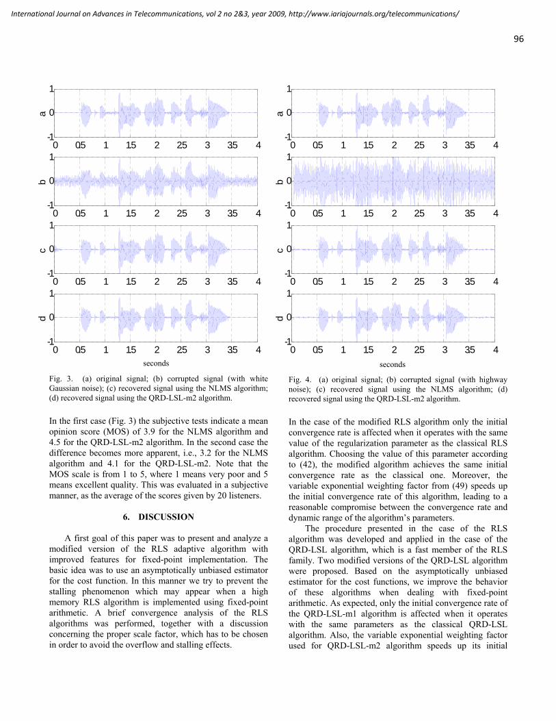
96


Fig. 3. (a) original signal; (b) corrupted signal (with white Gaussian noise); (c) recovered signal using the NLMS algorithm; (d) recovered signal using the QRD-LSL-m2 algorithm. In the first case (Fig. 3) the subjective tests indicate a mean opinion score (MOS) of 3.9 for the NLMS algorithm and 4.5 for the QRD-LSL-m2 algorithm. In the second case the difference becomes more apparent, i.e., 3.2 for the NLMS algorithm and 4.1 for the QRD-LSL-m2. Note that the MOS scale is from 1 to 5, where 1 means very poor and 5 means excellent quality. This was evaluated in a subjective manner, as the average of the scores given by 20 listeners.

6. DISCUSSION

A first goal of this paper was to present and analyze a

modified version of the RLS adaptive algorithm with improved features for fixed-point implementation. The basic idea was to use an asymptotically unbiased estimator for the cost function. In this manner we try to prevent the stalling phenomenon which may appear when a high memory RLS algorithm is implemented using fixed-point arithmetic. A brief convergence analysis of the RLS algorithms was performed, together with a discussion concerning the proper scale factor, which has to be chosen in order to avoid the overflow and stalling effects.

0 0.5 1 1.5 2 2.5 3 3.5 4-1

0

1

a

0 0.5 1 1.5 2 2.5 3 3.5 4-1

0

1

b

0 0.5 1 1.5 2 2.5 3 3.5 4-1

0

1

c

0 0.5 1 1.5 2 2.5 3 3.5 4-1

0

1

d

secundeseconds

0 0.5 1 1.5 2 2.5 3 3.5 4-1

0

1

a

0 0.5 1 1.5 2 2.5 3 3.5 4-1

0

1

b0 0.5 1 1.5 2 2.5 3 3.5 4

-1

0

1

c

0 0.5 1 1.5 2 2.5 3 3.5 4-1

0

1d

secundeseconds

Fig. 4. (a) original signal; (b) corrupted signal (with highway noise); (c) recovered signal using the NLMS algorithm; (d) recovered signal using the QRD-LSL-m2 algorithm. In the case of the modified RLS algorithm only the initial convergence rate is affected when it operates with the same value of the regularization parameter as the classical RLS algorithm. Choosing the value of this parameter according to (42), the modified algorithm achieves the same initial convergence rate as the classical one. Moreover, the variable exponential weighting factor from (49) speeds up the initial convergence rate of this algorithm, leading to a reasonable compromise between the convergence rate and dynamic range of the algorithm’s parameters.

The procedure presented in the case of the RLS algorithm was developed and applied in the case of the QRD-LSL algorithm, which is a fast member of the RLS family. Two modified versions of the QRD-LSL algorithm were proposed. Based on the asymptotically unbiased estimator for the cost functions, we improve the behavior of these algorithms when dealing with fixed-point arithmetic. As expected, only the initial convergence rate of the QRD-LSL-m1 algorithm is affected when it operates with the same parameters as the classical QRD-LSL algorithm. Also, the variable exponential weighting factor used for QRD-LSL-m2 algorithm speeds up its initial

97


convergence rate. The simulations performed in both Matlab and fixed-point DSP support the theoretical findings.

7. CONCLUSIONS

A class of RLS algorithms suitable for fixed-point implementation was presented in this paper. The proposed approach was applied in the case of the QRD-LSL algorithm. The performance of the resulted algorithm was evaluated in a noise reduction scenario, obtaining promising results.

8. REFERENCES [1] S. Haykin, Adaptive Filter Theory – Fourth Edition.

Prentice-Hall, Inc., Upper Saddle River, New Jersey, 2002.

[2] T. Adali and S. H. Ardalan, “Convergence and error

analysis of the fixed point RLS algorithm with correlated inputs,” Proc. of IEEE Int. Conf. on Acoustics, Speech, and Signal Processing, ICASSP 1990, vol. 3, pp. 1479-1482.

[3] I.K. Proudler, J.G. McWhirter, and T.J. Shepherd,

“QRD-based lattice filter algorithms,” Proc. SPIE, vol. 1152, pp. 56-67, 1989.

[4] J.-T. Yuan, “A modified QRD for smoothing and a

QRD-LSL smoothing algorithm,” IEEE Trans. Signal Processing, vol. 47, no. 5, pp. 1414-1420, May 1999.

[5] J.-T. Yuan and J.-N. Lee, “Narrow-band interference

rejection in DS/CDMA systems using adaptive (QRD-LSL)-based nonlinear ACM interpolators,” IEEE Trans. Vehicular Technology, vol. 52, no. 2, pp. 374-379, Mar. 2003.

[6] C. Paleologu, S. Ciochină, and A.A. Enescu, “A

network echo canceler based on a SRF QRD-LSL adaptive algorithm implemented on Motorola StarCore SC140 DSP,” Lecture Notes in Computer Science, Springer-Verlag, vol. 3124, pp. 560-567, June 2004.

[7] G. Rombouts and M. Moonen, “Fast QRD-lattice-

based unconstrained optimal filtering for acoustic noise reduction,” IEEE Trans. Speech and Audio Processing, vol. 13, no. 6, pp. 1130-1143, Nov. 2005.

[8] J.-T. Yuan, C.-A. Chiang, and C.-H. Wu, “A square-root-free QRD-LSL interpolation algorithm,” Proc. of IEEE Int. Conf. on Acoustics, Speech, and Signal Processing, ICASSP 2008, pp. 3813-3816, Apr. 2008.

[9] C. Paleologu, A. A. Enescu, S. Ciochină, and F. Albu,

“QRD-LSL Adaptive Algorithms Suitable for Fixed-Point Implementation,” Proc. IEEE Advanced International Conference on Telecommunications (AICT), pp. 163-167, Venice, Italy, May 2009.

[10] C. Paleologu, F. Albu, A. A. Enescu, and S. Ciochină,

“Modified SRF-QRD-LSL Adaptive Algorithm with Improved Numerical Robustness,” IARIA International Journal on Advances in Systems and Measurements, vol. 2, no. 1, pp. 56-65, 2009.

[11] J. Benesty and Y. Huang, Eds, Adaptive Signal

Processing--Applications to Real-World Problems. Springer-Verlag, Berlin, Germany, 2003.

[12] G. V. Moustakides, “Study of the Transient Phase of

the Forgetting Factor RLS,” IEEE Transactions on Signal Processing, vol. 45, no. 10, pp. 2468-2476, Oct. 1997.

[13] M. H. Verhaegen, “Round-off Error Propagation in

Four Generally-Applicable, Recursive Least-Squares Estimation Schemes,” Automatica, vol. 25, no. 3, pp. 437-444, 1989.

[14] S. Ciochină, C. Paleologu, and A.A. Enescu, “On the

Behaviour of RLS Adaptive Algorithm in Fixed-Point Implementation,” Proc. of IEEE Int. Symp. on Signals, Circuits and Systems, SCS 2003, vol. 1, pp. 57-60, July 2003.

[15] C. Paleologu, A. A. Enescu, and S. Ciochină,

“Recursive Least-Squares Lattice Adaptive Algorithm Suitable for Fixed-Point Implementation,” Proc of IEEE International Conference on Electronics, Circuits and Systems, ICECS 2006, pp.1105-1108, Dec. 2006

[16] E. Haensler and G. Schmidt, Eds., Topics in Acoustic

Echo and Noise Control. Springer-Verlag, Berlin, Germany, 2006.

[17] J. Benesty, J. Chen, Y. Huang, and I. Cohen, Noise

Reduction in Speech Processing. Springer-Verlag, Berlin, Germany, 2009.

98


Adaptive Rate Voice over IP Quality Management Algorithm

Eugene S. Myakotnykh Centre for Quantifiable Quality of Service in

Communication Systems (Q2S) 1, Norwegian University of Science and Technology,

Trondheim, Norway E-mail: [email protected]

Richard A. Thompson Telecommunications and Networking Program,

Department of Information Sciences and Telecommunications, University of Pittsburgh,

Pittsburgh, USA E-mail: [email protected]

Abstract—The quality of voice-over-IP communication relies significantly on the network that transports voice packets because this network does not usually guarantee available bandwidth, delay, and loss that are critical for real-time voice traffic. The solution proposed here is to manage a voice-over-IP stream dynamically, changing encoding parameters as needed to assure quality. The paper proposes an adaptive-rate control algorithm that establishes interaction between a VoIP sender and a receiver, and manages voice quality in real-time. Simulations demonstrate that the system provides better average communications quality than traditional fixed-rate VoIP.

Keywords-adaptive VoIP; E-model; Packetization; Speech quality; Voice-over-IP (VoIP)

I. INTRODUCTION A packet-switched network does not provide reliable

transport of real-time data: it does not guarantee available bandwidth, end-to-end delay and packet loss parameters, which are critical for real-time voice traffic. Most of the previous research in the VoIP quality has concentrated on networking issues of QoS management. Many different algorithms were developed to improve the transport of packetized voice traffic, including traffic classification (Differentiated Services technology [1, 2]), bandwidth reservation (Integrated Services architecture [3], Resource Reservation Protocol [4]), congestion avoidance, Multi-Protocol Label Switching technology [5], and others. These approaches use different techniques to decrease transmission delay and/or probability of voice packet congestion in the network and make the Internet more suitable for real-time traffic transmission. However, these methods often do not provide acceptable results nor do they solve the problem completely because (1) not all equipment and service providers support same QoS protocols and quality standards, and (2) the Internet is a dynamic media; the technologies often cannot react to changing network conditions and manage the quality of every communication session in real-time.

1 “Centre for Quantifiable Quality of Service in Communication Systems, Centre of Excellence” appointed by The Research Council of Norway, funded by the Research Council, NTNU and UNINETT. http://www.q2s.ntnu.no

The alternative approach is to adaptively manage voice encoding parameters on the sender side depending on the network conditions. A proper choice of a voice payload size or compression may enhance the quality of VoIP because it can dynamically change a configuration of a VoIP system, so that the system matches a current state of the network. This approach proposes to adjust a voice stream to the network and change parameters of the stream in real-time, depending on the network state.

This paper proposes an adaptive quality management mechanism that changes speech encoding parameters on the sender side in real-time depending on network impairments. This area is in the early stage of its development and investigation of many questions related to VoIP quality measurement and management, dependencies between multiple parameters and the resulting quality, is necessary to develop intelligent and efficient adaptive VoIP codecs.

When designing an adaptive quality management algorithm, several questions must be answered:

(1) Which factor (or factors) should be used to make a decision that a change of certain speech encoding parameters is required or not required at a given moment of time?

(2) How the end-user speech encoding parameters (packet duration and compression) affect VoIP quality under different network conditions. What encoding parameters should be changed and how to do it? How often should such a decision be made (per talkspurt, periodically, etc.)?

(3) How should feedback from the receiver be sent to the sender side?

Although this paper speaks about adaptive VoIP quality management and uses a set of narrowband voice codecs for analysis and as an example, the result and the approach can potentially be extended to a wider set of narrowband codecs, to wideband encoding and to IP-based audio in general.

This article is an extended version of paper [6] and it is organized as follows: the next Section provides an overview of related research in the area of adaptive VoIP. Section III describes network scheme and assumptions used in our simulation studies. Section IV investigates the effect of speech encoding parameters (packet size and compression/encoding variation) on quality of VoIP communications; Section V describes decision-making parameters for the proposed algorithm; Section VI shows the actual adaptive voice quality management mechanism. The results of the simulation study are presented in Section VII. Conclusion is drawn in Section VIII.

99


II. RELATED WORK

A. Adaptive Quality Management A number of studies investigating the idea of adaptive

voice quality management are available. Multiple papers (for example, Qiao et al. [7], Seo et al. [8], Matta et al. [9], and others) adopt the GSM/UMTS Adaptive Multi-Rate codec (AMR) [10] for the IP-network. The AMR codec was originally developed for wireless networks and the decision about adaptation of its encoding parameters is based on channel interference. The philosophy behind AMR is to lower a codec rate as the channel interference increases and thus enabling more error correction to be applied. Evidently, the process of adaptive quality management in the IP-network is different than that in wireless communications: there is no channel interference, there are IP packets instead of radio signals, and the threshold choice and management process will be different. The papers above present ideas of how to use the existing encoding scheme in the IP network.

A real-time change of speech encoding parameters can be achieved through variation of voice packet size or compression (encoding scheme). As the voice packet travels through the Internet, an overhead with control information is added to the voice payload. The size of overhead added to a voice packet is 40 bytes (the application layer Real-Time Transport Protocol (RTP) [11] header is 12 bytes; the transport layer UDP header is 8 bytes; and the IP header is 20 bytes), and it is significant compared to a typical voice payload size. If the G.711 codec [12] is taken as an example, the length of one 10-ms packet is 80 bytes. So, the RTP/UDP/IP overhead is 50% of the payload size and the total bandwidth required for the voice stream transmission is 96 kbps.

Changing end-user parameters may significantly affect bandwidth requirements per call and, as a result, its quality. For example, increasing a voice stream IP-rate will lead to increased quality, but the probability of quality degradation due to potential congestion may also increase because of higher channel capacity requirements. Several papers (for example, [13], [14], [15]) studied how changing of the encoding parameters affects VoIP communication quality.

Various parameters can be used to detect congestion in the network and make a decision about encoding parameters adaptation. For example, Bolot et al. [16] and Mohamed et al. [17] perform adaptive rate control based on packet loss statistics. The computational quality model called the E-model [18] is used in [9], [19] and [20]. Ngamwonwattana, [21] makes decision about codec rate adaptation based on moving average thresholds of delay and packet loss, and proposes sending control messages from the receiver “on demand”.

The recent paper of F. Sabrina and J. Valin [22] describes an adaptive mechanism using Speex codec [23]. The authors propose a novel criterion to get feedback about the network condition and a mechanism for adjusting the encoding bit rate based on the feedback and on instantaneous speech properties.

B. Voice-over-IP Quality Assessment This paper uses several metrics to estimate quality of

voice-over-IP communications. Voice quality measurement methodologies include subjective testing (involves human subjects and considered as the ultimate way of quality evaluation), and objective techniques (signals comparison or computational methods). The leading subjective criterion of voice quality measurements is the Mean Opinion Score (MOS), which is defined in the ITU-T Recommendation P.800 [24]. MOS is a score of voice quality as perceived by a large number of people listening to speech over a communication system. This Recommendation uses the scale from one to five and the MOS of some session of voice transmission is the average estimate of voice quality rates assigned by individual listeners (1 – bad, 2 – poor, 3 – fair, 4 – good, 5 – excellent). Subjective tests are usually complex and time-consuming and cannot be used for real-time quality assessment. Objective mechanisms are needed for this purpose.

Here in the project, the real-time decision about parameters adaptation is based on two computed metrics: an instantaneous quality level, which is measured per talkspurt using the computational E-model [18], and, in addition to this, a change of integral perceptual quality level, which is estimated based on a model developed by AT&T [25]. The original version of the E-model is relatively complex. It includes about 20 input parameters representing various terminal, network and environmental quality impairment factors. In the narrowband voice-over-IP area, the simplified version of this model is often used with default values for all but a few parameters - delay and packet loss. The model computes speech quality rating on a 100-point scale as:

R = R0 – Id – Ie-eff (1)

R is the resulting indicator of voice quality; R0 is the maximum score, achievable by codecs in the absence of loss and significant delay; Id is the impairment factor caused by end-to-end delay (a function of delay); Ie-eff is the effective equipment impairment factor, which depends on used codec, and also on packet loss rate and effectiveness of packet loss concealment algorithms. The E-Model is based on the concept that “psychological factors on the psychological scale are additive” [18]. It does not imply that the factors are uncorrelated, but only that their contributions to the estimated impairments are independent and each impairment factor can be computed separately. Numerical characteristics for different codecs and more details about the model can be found in [18], [26], [27]. A similar model for wideband telephony is proposed in [28].

The E-model uses a special mapping function to establish a relationship between the 100-point R-scale and the traditional MOS scale (Equation 2).

MOS =1+ 0.035R + R(R − 60)(100 − R) ·7·10-6 (2)

This model is not a perfect tool to calculate absolute quality level, but it is acceptable for measuring variations in quality.

100


Detailed investigations of this question by NTT Lab (Japan) [29] concluded that correlation coefficient of results provided by the E-model with subjective human testing results is about 80%. Since, goal of these algorithms is to achieve noticeable relative quality improvement, the E-model can be used to track changes in quality.

The E-model estimates average quality during a certain period of time. But quality, as perceived by the end-user, depends not only on significance of a quality distortion, but also when this distortion happened during a communication session. The effect, which reflects the way that a listener remembers call quality, is called “recency” effect. This effect implies that periods of low or high quality positioned at the end of a speech sample have a stronger influence on the overall session quality then when such periods are positioned in the beginning of the sample. In tests conducted by AT&T [25], a burst of noise was created and moved from the beginning to the end of a 60-second call. When the noise was at the start of the call, users reported a higher MOS score than when the noise was at the end of the call. Tests reported by France Telecom [30] showed a similar effect. The effect is believed to be due to the tendency for people to remember the most recent events or possibly due to auditory memory, which typically decays over a 15-30 second interval [30].

Further discussion about these parameters will be provided below. Using these metrics, the novel mechanism to adaptively manage speech encoding parameters is proposed.

III. SIMULATION DESIGN

A. Network Model The proposed adaptive speech quality management

algorithm is tested using a simulation implemented in Matlab. The network topology for the simulation is shown in Fig. 1. A simplified scenario with a single place of potential congestion is analyzed. The congestion may be caused by bursty background traffic through the router. The link capacity is 5 Mbps, but, actually, this number is not very important. But, a portion of voice and data traffic in the network is important: a significant difference in VoIP quality is seen over the same network, with the same total (voice plus data) average traffic load, but with different voice-to-data traffic ratios. The presence of large data packets with bursty behavior creates “instability” in the voice transmission process, which causes additional delay variation (jitter) and, as a result, higher delay and/or packet loss. The

propagation and network processing delay is assumed fixed at 50 ms (it may be noticeably higher in real networks). The bottleneck router uses FIFO queuing and the drop-tail mechanism in case of overflow. The router has a finite queue size (64 Kbyte), enough to keep packets in queue for about 100 milliseconds.

B. Voice Encoding This project uses parameters of three narrowband codecs

for developing and simulating the proposed adaptive quality management scheme: the G.711 [12] (PCM encoding with no compression), the G.726 [31] (ADPCM encoding with 2:1 compression), and the G.729a [32] (CS-ACELP encoding with 8:1 compression). While codec may have different voice payload sizes, the discrete values 10 ms, 20 ms, 30 ms will be used. So, nine different sets of encoding parameters are used. These codecs and parameters are chosen for analysis because: 1) they provide a relatively high level of quality (higher than or close to the toll-grade); 2) their quantitative characteristics are known in terms of maximum encoded speech quality in the absence of packet loss and significant delay [18]; and 3) the difference in channel capacity consumption in these codecs is significant: for example, the G.711 codec with 10 ms voice payload size requires 96 kbps per stream (64 kbps of audio bit rate and 32 kbps to send the RTP/UDP/IP overhead); the 30 ms G.729 codec needs just 18.7 kbps channel (8 kbps audio rate and 10.7 kbps overhead bit rate). Selecting one of the nine sets of encoding parameters will be based on metrics calculated on the receiver side. These codecs are chosen as examples; similar adaptive mechanisms can be used with a different set of narrowband codecs, with some set of wideband codecs or with a combination of narrowband and wideband codecs.

C. Call Characteristics It is assumed that speech codecs with variable parameters

(packet size, compression) are used. Delay and packet loss statistics is calculated on the receiver side. The E-model [18] is applied to get a quality metrics based on these parameters. The E-model parameters for the selected codecs are defined in [18] and [27]. Simulated call duration is 120 seconds. Silence suppression is not used (for simplicity). Voice stream may include a single call or a group of calls (aggregated voice traffic). All calls in the group use the same speech encoding algorithm; calls can be managed simultaneously; and all have the same behavior (the quality of all calls degrades equally).

Figure 1: Simulated network structure

101


D. Background Traffic Modeling It is desirable to generate background traffic with

characteristics similar to traffic patterns in the Internet. Studies revealed that Internet traffic exhibits properties of (1) self-similarity, (2) burstiness and (3) long-range dependency (LRD) [33]. The self-similar process shows that short-time traffic behavior patterns are close to long-time patterns. LRD means that there is a statistically significant correlation across large time-scales [34]. In [35, 36], it is suggested to use multiple Pareto aggregation sources with a Pareto index parameter a < 2. Our study uses this approach by generating Pareto On/Off traffic from 10 different sources. The traffic from each source consists of sending packets at a fixed rate only during the On periods, whereas the Off periods are idle. The packet sizes are: 64 bytes (60% of packets), 550 bytes (25% of packets) and 1500 bytes (15% of packets). The aggregated traffic will have all the required characteristics. The Network Simulator NS-2 [37] also uses this model of background traffic generation.

It is important that the model does not separate the generated traffic into TCP and UDP flows. But the approach is good to model Internet traffic behavior, even in congested networks, ignoring nonlinearities arising from the interaction of multiple traffic sources because of network resource limitations and TCP’s feedback congestion control algorithm [38]. One possible reason is that more than 90 percent of TCP sessions in the Internet are very short (1-2 seconds) and exchange less than 10 Kbytes of data [39].

According to recent research [40, 41], the nature of traffic in the Internet changes because of a significant increase of peer-to-peer traffic and assumptions used in this section may not be true in future. The proportion of peer-to-peer traffic in the network increased significantly during the last several years and achieves 50% of the total traffic. This fact may change two assumptions: a) the packet-size distribution of the Internet traffic will change; b) TCP session will exchange more data, will be longer and the TCP back-off mechanism should be simulated. This study uses the On/Off Pareto model and the TCP-based model will be analyzed in future.

E. Jitter Buffer Management Jitter is a variation in packet transit delay caused by

queuing and serialization effects on the path through the network. It is eliminated by jitter buffers, which temporarily store arriving packets and send them to a receiver in equal intervals. The buffer may have a fixed size, but if is too small, a lot of packets may be discarded because of a significant delay variation. This will negatively affect speech quality. Increasing the jitter buffer allows waiting longer for delayed packets but increases the overall end-to-end delay, which also negatively affects speech quality. A lot of research focuses on adaptive jitter buffer strategies to find some optimal point in the tradeoff between the end-to-end delay and packet loss and to optimize speech quality dynamically.

The basic adaptive playout algorithm of Ramjee et al. [42] is used in the simulation. It calculates two statistics to make a jitter buffer adaptation decision. For each arriving

packet, it computes the expected mean and variation in the end-to-end delay (di and υi. respectively). Specifically, the end-to-end delay estimate for packet i is computed as

di = α·di-1 + (1-α)·ni (3)

where ni is the i-th packet delay. The variation is: as:

υi = α·υi-1 + (1-α)·| di – ni | (4) Packet playout time in this algorithm is calculated as:

pi = ti + di + βυi (5) where ti is the time the packet was sent. α = 0.875 and β=4.

While these equations estimate di and υi for each packet, playout time pi is adjusted only in the intervals between talkspurts (periods of speech). Different papers use periods between 200 and 700 ms to describe talkspurt durations and there is no agreement about the “best” number. The ITU P.59 [43] recommendation specifies an artificial on/off model for generating human speech with the talkspurts and silence intervals of 227 ms and 596 ms. Jiang and Schulzrinne [44] reported mean spurts and gaps of 293 ms and 306 ms in experiments with the G.729 codec. The durations of 300 ms both for silence and active speech periods are used in the simulation.

IV. THE EFFECT OF END-USER PARAMETERS ON VOIP QUALITY

A. Effect of Background Traffic on VoIP Quality Before investigating the effect of the parameters on

speech quality, it is important to demonstrate that the quality is affected by not only high link utilization, but also by the proportion of voice and data traffic in the network. This hypothesis is rather evident: the data traffic is bursty and it may cause a sudden congestion in the network, which results in higher delays and/or losses of voice packets.

The simulation design is based on the network scheme and the assumptions described in the previous section. The narrowband G.711 codec with 64 kbps of audio bit rate is used in the example. Speech quality is measured in MOS depending on the total link utilization U (voice and data traffic; average during the call) and D (ratio of data traffic and total mixed traffic). Note that U is not an average ISP network utilization; this is a utilization of the bottleneck link during the considered 120-second simulation. The results and the standard deviations are presented in Fig. 2.

The results show that the behavior of voice traffic significantly depends on the presence of, and load of, the data traffic in the network. Even a relatively small volume of data traffic can cause a significant degradation of voice traffic. While this conclusion is intuitively clear, the simulation study gives numerical estimates. If the average link utilization exceeds 70%, adaptive quality management mechanisms can potentially be used and change of packet size and/or speech compression may decrease the quality degradation effect. But, this number (70%) depends on the

102


assumptions and will be slightly different with other adaptive jitter buffer algorithms, different approaches for background traffic generation, and assumptions about talkspurt duration

0 0.2 0.4 0.6 0.8 1

3

3.2

3.4

3.6

3.8

4

4.2

4.4

Data traffic / Total traffic

MO

S

U = 0.8

U = 0.9

U = 1.0

U = 0.7

Figure 2: Speech quality depending on traffic structure

It is necessary to understand that, in most cases, the structure of traffic in the network (in the congested router) is not known and not possible to measure (unless a user or a provider controls all hardware devices along a path of a given call). But the results of the study presented below still helpful in understanding of how variations of voice stream parameters affect its quality and in which scenarios the end-user codec adaptation may be beneficial.

B. Effect of Packet Size Variation on VoIP Quality The effect of packet size variation is difficult to describe

theoretically because many of the parameters affecting quality (delay, loss, jitter) are not independent and improving one parameter may cause a decline in another. Some effects of packet size on speech quality are very clear, others are less evident. Four main relationships are identified:

(1) Increasing packet size leads to an increase of end-to-end delay. If the delay is not too large, the direct impact of packet size increase is very small and not perceptually noticeable [18]. But, if the delay is significant, an additional increase of packet duration may be noticeable.

(2) Increasing packet size leads to decrease of the IP-rate per call. This may decrease congestion in the network and improve the quality of communication. The dependency is also evident and the question about the effectiveness of voice transmission was briefly discussed in Section 2.

There are two less evident, but also important effects of packet size variation on VoIP quality:

(3) A loss of one “long” packet has more significant negative effect on speech quality than a random loss of several “small” packets. Mathematical representation of this effect in the E-model can be found in [18].

(4) In presence of data traffic in the network, increase of voice packet size decreases link utilization, but increases the data-to-voice traffic ratio. As demonstrated in the previous section, this may cause additional “instability” in the

network, which may result in higher jitter, delay or loss. This factor may affect the resulting speech quality, but it is not clear how significant the effect might be.

It is seen that increasing packet size causes different effects on the speech quality. Since, the result is difficult to predict theoretically, it is investigated using simulation. The portions of voice (number of calls) and data traffic in the network were changed, and the average call quality was measured for different packet sizes. Speech quality is measured in MOS depending on the portion of voice traffic in the network V, the total link utilization U (average during the call) and the packet size PS (changes from 10 to 50 ms). For each combination of {V, U, PS}, 100 experiments were run. The standard deviation of MOS scores does not exceed 0.15 MOS. The simulation results for several specific values of V (portion of voice traffic) are shown in Fig. 3.

Figure 3: Effect of packet size on VoIP quality

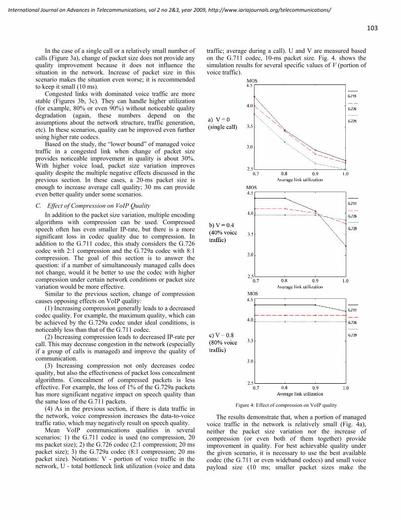
103


In the case of a single call or a relatively small number of calls (Figure 3a), change of packet size does not provide any quality improvement because it does not influence the situation in the network. Increase of packet size in this scenario makes the situation even worse; it is recommended to keep it small (10 ms).

Congested links with dominated voice traffic are more stable (Figures 3b, 3c). They can handle higher utilization (for example, 80% or even 90%) without noticeable quality degradation (again, these numbers depend on the assumptions about the network structure, traffic generation, etc). In these scenarios, quality can be improved even further using higher rate codecs.

Based on the study, the “lower bound” of managed voice traffic in a congested link when change of packet size provides noticeable improvement in quality is about 30%. With higher voice load, packet size variation improves quality despite the multiple negative effects discussed in the previous section. In these cases, a 20-ms packet size is enough to increase average call quality; 30 ms can provide even better quality under some scenarios.

C. Effect of Compression on VoIP Quality In addition to the packet size variation, multiple encoding

algorithms with compression can be used. Compressed speech often has even smaller IP-rate, but there is a more significant loss in codec quality due to compression. In addition to the G.711 codec, this study considers the G.726 codec with 2:1 compression and the G.729a codec with 8:1 compression. The goal of this section is to answer the question: if a number of simultaneously managed calls does not change, would it be better to use the codec with higher compression under certain network conditions or packet size variation would be more effective.

Similar to the previous section, change of compression causes opposing effects on VoIP quality:

(1) Increasing compression generally leads to a decreased codec quality. For example, the maximum quality, which can be achieved by the G.729a codec under ideal conditions, is noticeably less than that of the G.711 codec.

(2) Increasing compression leads to decreased IP-rate per call. This may decrease congestion in the network (especially if a group of calls is managed) and improve the quality of communication.

(3) Increasing compression not only decreases codec quality, but also the effectiveness of packet loss concealment algorithms. Concealment of compressed packets is less effective. For example, the loss of 1% of the G.729a packets has more significant negative impact on speech quality than the same loss of the G.711 packets.

(4) As in the previous section, if there is data traffic in the network, voice compression increases the data-to-voice traffic ratio, which may negatively result on speech quality.

Mean VoIP communications qualities in several scenarios: 1) the G.711 codec is used (no compression, 20 ms packet size); 2) the G.726 codec (2:1 compression; 20 ms packet size); 3) the G.729a codec (8:1 compression; 20 ms packet size). Notations: V - portion of voice traffic in the network, U - total bottleneck link utilization (voice and data

traffic; average during a call). U and V are measured based on the G.711 codec, 10-ms packet size. Fig. 4. shows the simulation results for several specific values of V (portion of voice traffic).

Figure 4: Effect of compression on VoIP quality

The results demonstrate that, when a portion of managed voice traffic in the network is relatively small (Fig. 4a), neither the packet size variation nor the increase of compression (or even both of them together) provide improvement in quality. For best achievable quality under the given scenario, it is necessary to use the best available codec (the G.711 or even wideband codecs) and small voice payload size (10 ms; smaller packet sizes make the

104


communication process very inefficient). If portion of managed voice traffic is more significant, changing packetization provides better resulting speech quality than compression variation (until a certain level of the bottleneck link utilization) despite the fact that the compressed speech uses less channel capacity (Fig. 4c). Only when the bottleneck link is very heavily congested (more than 90%), the compressed encoding provides better quality (Fig. 4b).

D. Summary The presented results are based on assumptions about

network structure, background traffic pattern, speech characteristics (talkspurt duration), which are described in the previous section. Other jitter buffer algorithms or, for example, a different model of speech representation (talkspurt and silence periods) will change numerical results, but the general conclusion will remain the same: in congested networks try to manage voice payload size first, because it may provide higher resulting quality than codecs with compression; if this does not help – change a voice stream bit rate using both higher compression and packet size variation. The results are consistent with other studies mentioned in Section 2, but provide approximate quantitative criteria when end-user variation of encoding parameters may be effective for average call quality improvement.

This study had assumed that average background traffic load in the network is known. In real networks this information is not available to the end-points, so mechanisms would be needed to estimate the effect of the network on communication quality. Monitoring a call or a group of calls on the receiver side, we do not know average link utilization and average volume of background traffic in the network. Number of simultaneously managed calls is known, but this information is not too important: the quality depends on the proportion of data traffic in the network and, even if there are many calls, often it cannot be said with high confidence whether the network is voice-only or even if voice traffic dominates in the network. For this reason, the conclusions from this part cannot be used directly.

It is important to remember that two adaptive mechanisms are going to work simultaneously: a) the proposed variable sender-based encoding mechanisms and b) the receiver’s adaptive jitter buffer. The adaptive jitter buffer mechanism is used to improve short-term quality (its fast reaction does not change the encoding characteristics, but manages the delay-loss tradeoff). Sender-based management is designed to improve long-term voice flow characteristics (to choose the encoding scheme that best matches the given network conditions).

V. DECISION-MAKING PARAMETERS FOR ADAPTIVE SPEECH QUALITY MANAGEMENT

Which parameters should be taken into account to make a decision about quality adaptation? One variant is to use, for example, the mean delay, the moving average delay, or loss statistics. This approach has already been used in several papers mentioned above. It would not be acceptable to analyze these parameters separately: high packet loss definitely means a significant degradation in quality but low

(or absence of) packet loss does not mean an absence of degradation because the adaptive jitter buffer size can be very significant and we can get high end-to-end delay instead of the loss. So, it would be better to use these parameters together. In other words, one must measure quality, which depends on end-to-end delay, loss, and codec characteristics. This project does not analyze some “less evident” parameters affecting speech quality like echo, attenuation, noise in a channel, etc. The quality can be measured using the computational E-model [18].

How can this model be used? The adaptive algorithms proposed here will measure and manage quality-per-talkspurt. Human communication consists of periods of active speech and periods of silence. The adaptive jitter buffer algorithm changes its buffer size in periods between talkspurts (during silence periods). So, it would be logical to analyze speech quality behavior, and to make decisions about adaptive quality management at the end of a talkspurt (at the end of an active speech period). The E-model can be used to calculate the quality of each talkspurt (referred to as “instantaneous quality”). Packets within a talkspurt have the same end-to-end delay; network loss and jitter buffer loss can easily be counted. The difference between instantaneous quality levels in two consecutive talkspurts can be very significant because of the bursty nature of the background traffic.

But, knowledge of instantaneous call quality is not enough to make a decision about changing the speech encoding parameters. Measurable voice quality can change significantly and immediately but it takes some time for users to understand that the quality has changed. Perceptual (real) speech quality is different from an instantaneous computational quality. Perceptual quality takes into account factors not only during the last short period of time (last second or several seconds), but all quality values and quality variation history starting at the beginning of a call [45]. So, in addition to the computational quality model, it would be useful to estimate (1) instantaneous perceptual speech quality at any moment of time during a call, and (2) integral quality at any moment of time during a call.

The E-model can also be used to measure the average call quality at a given moment of time during a conversation. This metric would probably be acceptable, but this project tries a different approach, using a metric, that describes integral (total) speech quality. Integral quality that is calculated as a mean of instantaneous qualities is not a very good metric. This model does not take into account the history of previous quality variations (frequent variations may result in a relatively high average quality but noticeably smaller real perceptual quality).

Instead of using just a mean MOS metric, integral quality is calculated from the beginning of a call using the perceptual model of Rosenbluth [25]. This model presents a call as a sequence of 8-second intervals. Quality within each interval is calculated as a mean of instantaneous qualities. Integral call quality is calculated as a weighed sum of the qualities of the longer intervals and reflects an opinion that quality levels at the end of a conversation have higher weights on the overall perceived call quality than quality

105


levels at the beginning of a session. Perceptual quality is usually lower than the average computational quality if there are frequent variations of instantaneous quality levels. This model was justified by subjective experiments performed by AT&T. It is proposed to use the weighting average with weights

{ }⎢⎣⎡

⎥⎦⎤−⋅⋅++= ⋅+ 2.1

61.096.0

68.0 )3.4()3.1038.0(1 ,1 max iLiii MOSLW (6)

∑∑ ⋅

=

ii

iii

IW

MOSW

MOS (7)

MOSI is the integral perceptual call quality; MOSi is the MOS during the shorter measurement period; Li is a location of a degradation period (measured on 0-to-1 scale; 0 indicates the beginning of a conversation, 1 is the end of a conversation; the parameter changes proportionally to time starting from the beginning of a call).

This perceptual call quality metrics will be used as one of decision parameters for adaptive speech quality management. If there are concerns about this model, it is possible to calculate the integral quality using weighted average with exponentially distributed weights described in [45]. The idea in Equations 6 and 7 is similar; the representation is a little bit more complex than just the exponentially distributed weighting.

VI. ADAPTIVE VOIP QUALITY MANAGEMENT ALGORITHM This section describes the proposed adaptive quality

management mechanism. The following section provides and example and results of a simulation study.

Step 1: Collect statistics of packet delays before the jitter buffer. If there are multiple calls, is assumed that the quality degradation pattern of all calls to be similar (this assumption is confirmed by our preliminary simulations). So, just one call from aggregated voice traffic may be chosen for analysis.

Step 2: Calculate packet playout time (Section 3E). This parameter is calculated continuously for each arrived packet but, since the jitter buffer is adjusted only in pauses between talkspurts (between active speech periods), the end-to-end delay is constant within a talkspurt.

Step 3: Calculate the quality of a talkspurt based on the E-model. This calculation includes: (1) calculating packet loss within a talkspurt (network and jitter buffer loss); (2) measuring end-to-end delay, which is constant within a talkspurt. This “quality per talkspurt” is referred as “instantaneous quality” and denoted it as QI. The difference between instantaneous quality levels in two consecutive talkspurts can be very significant because of the bursty nature of the background traffic. But, knowledge of this instantaneous call quality is not enough to make a decision about adaptation of speech encoding parameters.

Step 4: Calculate the maximum achievable quality level for a given codec under the given network conditions. This calculation is based on zero packet loss and minimum network delay (the sum of transmission delay, propagation delay and minimum queuing delay). This delay is taken from the analysis of incoming packets delays. Using this minimum network delay, calculate the maximum achievable quality under the given set of encoding characteristics:

R = R0 – Ie-eff – Id

Id = min. network delay + min. jitter buffer delay

MOS =1+ 0.035R + R(R − 60)(100 − R) ·7·10-6 (8)

MOS is a Mean Opinion Score on the 1-to-5 scale; R is the indicator of voice quality (the 100-point scale) from the computational E-model, R0 = 93.2 is the maximum achievable narrowband quality, Id is a function of delay; Ie-eff describes impairments related with encoding (codec quality) and packet loss. See the E-model standard [18] for more details about voice quality calculation. The result looks something like in Fig. 5:

Figure 5: Instantaneous speech quality measurement

Step 5: Continuously calculate the integral voice quality

level based on the model expressed by Equations 6 and 7.

Step 6: Decision. The proposed quality management scheme uses three parameters: 1) instantaneous quality level – QI; 2) integral perceptual quality – QT; and 3) maximum quality level achievable under the given set of speech encoding parameters – QM. If the number of managed calls (which is assumed to be known) is not significant (for example, one or two), voice flow is concluded to have an insignificant effect on the network, and it would be better to use the best available codec from the very beginning and not to use any quality adaptation strategies.

Similar to [7], two thresholds are used in the algorithm:

0.25 MOS and 0.5 MOS. These thresholds are used only to describe integral quality variation and these numbers are not chosen arbitrarily. A change in quality of 0.2-0.25 MOS is not too significant, but is noticeable by some people; smaller changes in quality are noticeable only by a relatively small percentage of listeners. A change in quality of about 0.5 MOS is very significant and is noticeable by almost everybody. If the best narrowband G.711 codec is used and its quality decreases by 0.5 MOS, the resulting quality will be lower than the toll-grade quality level. If the G.729 codec

106


is used and its quality degrades by 0.5 MOS, the resulting level of speech quality (about 3.4-3.5 MOS) is considered to be low by most people.

The situation with thresholds for instantaneous quality level is a little more complex. Talkspurt quality can decrease for two reasons: 1) high jitter buffer size, which results in high end-to-end delay and, usually, not significant loss, or 2) packet loss (usually not in the network but on a receiver size caused by significant delay variation and insufficient jitter buffer size). The effect of delay is generally lower: for example, with 150 ms of network and packetization delay and an additional 80 or 100 ms of jitter buffer size, the decrease in quality is about 0.3-0.4 MOS. But, if a bursty loss of packets causes a loss of, for example, only 3 out of 30 packets in a given talkspurt, the decrease in the instantaneous quality equals to 0.9 MOS. If 5 packets out of 30 are discarded, the resulting quality (for the G.711 codec) will be only 2.65 MOS (with a maximum level of 4.3-4.4 MOS). As in the case of integral quality, two thresholds are used: 0.3 and 1.0. If the difference between maximum and instantaneous quality levels does not exceed 1.0 on the MOS scale, the observed packet loss is considered reasonable.

This model does not use quality adaptation mechanisms during the first several seconds of conversation because the perceptual quality model expressed by Equations 7 and 8 is very sensitive to quality variations in the beginning of a call. In the simulation, this period is set to 8 seconds.

The details of the algorithm follow. Consider the differences between two parameters: 1) between the maximum and integral qualities (QM – QT), and 2) between the maximum and instantaneous quality levels (QM – QI). The first difference quantifies total quality variation; the second one describes instantaneous quality changes.

Condition 1:

if QM – QT > 0.5 // Low or unacceptable level of quality. Something has to be done immediately

o if QM – QI > 1.0 // Instantaneous quality level is also

very low. Not too much can be done in this situation. Switch to the G.729 codec with 30 ms packet size (the worst codec using the minimum IP-rate)

Action: switch to the G.729 codec, 30 ms packet size

o if 0.3 < QM – QI < 1.0

Action: keep current settings expecting that adaptive buffer will compensate the degradation

o if QM – QI < 0.3 // Total quality is very low, but

instantaneous quality level is close to maximum. Quality degradation is not seen, so start slowly to improve the codec quality by deceasing packet size

Action: decrease packet size by 10 ms if a current size is higher

Condition 2:

if 0.2 < QM – QT < 0.5 // Degradation of quality is noticeable, try to improve the situation

o if QM – QI > 1.0 // Have a long bursty loss of packets.

The network is significantly congested. Action: use codec with higher compression: if current codec is G.711, switch to G.726; if current codec is G.726, switch to G.729

o if 0.3< QM – QI < 1.0 // Also, the situation is not

good and bursty packet loss is observed Action: increase packet size by 10 ms or change codec if current packet size is 30 ms (maximum)

o if QM – QI < 0.3 // Instantaneous quality is

good; expect integral quality improvement Action: decrease packet size by 10 ms if a current size is higher

Condition 3:

if QM – QT < 0.2 // Degradation of quality is not significant but might be noticeable; try to improve the situation

o if QM – QI > 1.0 // Significant quality degradation.

Total quality is good but one more bursty loss can significantly drop overall quality. Try to avoid.

Action: increase packet size by 10 ms up to 30 ms

o if 0.3 < QM – QI < 1.0 // Assume that this decrease of

quality is temporal and due to single loss or increase of end-to-end delay

Action: keep current settings

o if QM – QI < 0.3 // Everything is fine: both total and instantaneous qualities are high.

Action: decrease packet size up to minimum or switch to a better codec

The algorithm is summarized in Table 1.

Step 7: To change current encoding algorithm according to the decision.

The actions defined above cannot be executed immediately. The collected information about instantaneous and integral quality levels has to be transmitted to the sender. The transmission delay can be significant in congested networks. Assume that three consecutive talkspurts on the sender side (TS1, TS2, TS3) are separated by periods of silence (S1, S2). According to assumptions in Section 3, the mean durations of the active speech and silence period are

107


TABLE I: THE ALGORITHM SUMMARY

Q(M)–Q(T) Q(M)-Q(I)

≤ 0.2 0.2 < … < 0.5 ≥ 0.5

≤ 0.3

- if current packet size is higher than 10 ms,

decrease it - if current size is 10 ms but used codec is not the G.711, switch to a better

codec

- decrease packet size up to 10 ms

- if current packet size is lower than 30 ms, increase it

0.3 < … < 1.0

- keep current settings

- if current packet size is lower than 30 ms, increase it

- if used codec is not G.729, switch

to a codec with higher

compression

≥ 1.0 - if current packet size is

lower than 30 ms, increase it

- if used codec is not G.729, switch

to a codec with higher

compression

- switch to the G.729 codec with 30 ms packet size

300 milliseconds. Assume that the receiver gets TS1 and makes a decision to send some control information to the sender. The period of time between the departure of the TS1 talkspurt and the arrival of the feedback from the receiver is equal to a round-trip delay (RTT). In congested networks this RTT might be significant and longer than the period of silence between the TS1 and TS2 talkspurts. In this case, the decision about quality adaptation will not be applied to the second talkspurt (TS2); it would be applied to TS2 only if the RTT is less than the S1 duration (300 ms). So, the receiver would not see the result of the requested changes of speech encoding parameters until the TS3 talkspurt, about one second later. The minimum reaction time of the algorithm is 300 ms (when RTT ≤ 300 ms). If the assumptions about speech/silence duration are different, these numbers will change respectively.

This fact has to be taken into account in the adaptation scheme. So, a restriction is added that, if a receiver analyzes a talkspurt (for example, TS1) and sends a control message to the sender to change speech encoding parameters, the next control message cannot be sent after the next consecutive talkspurt.(TS2); but only after analyzing of TS3, if it is required. This restriction provides more stability to the algorithm.

One more restriction is added. If a decision is made about several consecutive improvements of speech encoding parameters (for example, to decrease the voice payload size from 30 ms to 20 ms and then to 10 ms or to replace a given codec by a better codec) these changes should not be made too quickly because each change causes noticeable increase of IP-rate per call and thus, a higher probability of degradation due to congestion. The preliminary experiments showed that the system is more stable if the receiver waits for four talkspurts (about 2 seconds) between such decisions.

In sender-based control, observations about the network and resulting speech quality must be reported back to the sender. Utilizing RTCP is a common approach: packet loss

and delay variation statistics are included in RTCP reports. These packets are sent periodically, usually every 5 seconds. But, obviously, this type of control is very slow to respond to the network. If the control mechanism must make decisions more frequently, it is necessary to use a different scheme rather than RTCP. But more frequent periodic call control may introduce additional traffic in the network. The paper assumes that the adaptive quality management mechanism sends control messages, not periodically, but on demand, that is, when a change of sender parameters is required. As the simulation results will demonstrate, a decision to vary the encoding parameters is made less frequently than per talkspurt. Also, if a group of calls is managed, just one message can be sent to deliver feedback from the receiver, but not to control every call independently. This approach will not create a significant amount of additional control traffic in the network

VII. SIMULATION RESULTS

A. Example Fig. 6 demonstrates an example of the statistics collected

in one of the simulations. The first picture shows the packet delay and the jitter buffer size calculated in Step 2. If packet delay (blue line) is higher than jitter buffer size (red line), the packet is lost (discarded) and restored using a current codec’s packet loss concealment mechanism. The second figure demonstrates instantaneous (per talkspurt) speech quality (blue line, Step 3) and integral (perceptual) quality (red line, Step 5). The third picture shows the background traffic rate averaged over 10 ms intervals, and also the average long-term traffic rate.

Figure 6: Measured speech quality statistics

Figures 7 shows the quality of the VoIP stream when

exactly the same background traffic pattern exists and the stream is managed by the proposed adaptive quality

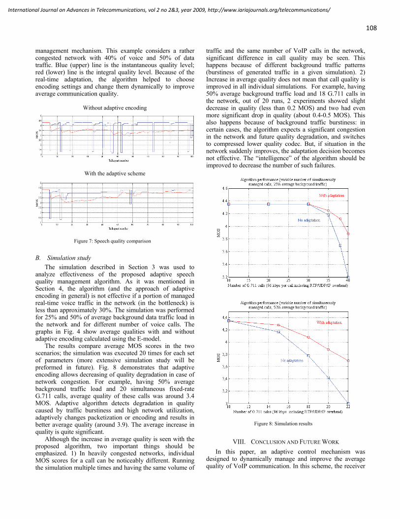
108


management mechanism. This example considers a rather congested network with 40% of voice and 50% of data traffic. Blue (upper) line is the instantaneous quality level; red (lower) line is the integral quality level. Because of the real-time adaptation, the algorithm helped to choose encoding settings and change them dynamically to improve average communication quality.

Without adaptive encoding

With the adaptive scheme

Figure 7: Speech quality comparison

B. Simulation study The simulation described in Section 3 was used to

analyze effectiveness of the proposed adaptive speech quality management algorithm. As it was mentioned in Section 4, the algorithm (and the approach of adaptive encoding in general) is not effective if a portion of managed real-time voice traffic in the network (in the bottleneck) is less than approximately 30%. The simulation was performed for 25% and 50% of average background data traffic load in the network and for different number of voice calls. The graphs in Fig. 4 show average qualities with and without adaptive encoding calculated using the E-model.

The results compare average MOS scores in the two scenarios; the simulation was executed 20 times for each set of parameters (more extensive simulation study will be preformed in future). Fig. 8 demonstrates that adaptive encoding allows decreasing of quality degradation in case of network congestion. For example, having 50% average background traffic load and 20 simultaneous fixed-rate G.711 calls, average quality of these calls was around 3.4 MOS. Adaptive algorithm detects degradation in quality caused by traffic burstiness and high network utilization, adaptively changes packetization or encoding and results in better average quality (around 3.9). The average increase in quality is quite significant.

Although the increase in average quality is seen with the proposed algorithm, two important things should be emphasized. 1) In heavily congested networks, individual MOS scores for a call can be noticeably different. Running the simulation multiple times and having the same volume of

traffic and the same number of VoIP calls in the network, significant difference in call quality may be seen. This happens because of different background traffic patterns (burstiness of generated traffic in a given simulation). 2) Increase in average quality does not mean that call quality is improved in all individual simulations. For example, having 50% average background traffic load and 18 G.711 calls in the network, out of 20 runs, 2 experiments showed slight decrease in quality (less than 0.2 MOS) and two had even more significant drop in quality (about 0.4-0.5 MOS). This also happens because of background traffic burstiness: in certain cases, the algorithm expects a significant congestion in the network and future quality degradation, and switches to compressed lower quality codec. But, if situation in the network suddenly improves, the adaptation decision becomes not effective. The “intelligence” of the algorithm should be improved to decrease the number of such failures.

Figure 8: Simulation results

VIII. CONCLUSION AND FUTURE WORK In this paper, an adaptive control mechanism was

designed to dynamically manage and improve the average quality of VoIP communication. In this scheme, the receiver

109


makes a control decision based on two parameters: 1) the computational instantaneous quality level, which is calculated per talkspurt using the E-model and 2) the perceptual metric, which estimate the integral speech quality by taking into account the fact that a decrease of communication quality depends, not only on the presence of packet delay or loss in the network, but also on the position of a quality degradation period in the call.

The algorithm works together with the adaptive jitter buffer mechanism. The adaptive jitter buffer is used to manage short-term quality; the sender-based adaptation technique tries to choose encoding parameters to improve a long-term quality by decreasing network congestion and, as a result, significant instantaneous changes in quality.

The paper uses three narrowband codecs with different packet sizes for analysis but the approach can be extended to a wider set of narrowband codecs, to wideband encoding schemes and, potentially, to IP-based audio in general.

Several questions will be addresses in the future work. First, it is necessary to work more on the algorithm and to decrease a number of cases when adaptive encoding makes a situation with quality worse. Second, according to recent research, the nature of traffic in the Internet changes because of significant increase of peer-to-peer traffic and assumptions about background traffic modeling used in Section 3 may not be true in future. Other traffic models simulating TCP backoff mechanism and/or mix of TCP and UDP traffic should be studied. Third, an adaptive change of speech encoding parameters affects perceptual quality. The proposed algorithm tried to avoid rapid changes of codecs and make adaptation as smooth as possible, but the question about what users hear when encoding parameters are changed and how this variation affects user feeling about a call, should also be investigated in more detail.

REFERENCES [1] RFC 2474, “Definition of the Differentiated Services Field (DS Field)

in the IPv4 and IPv6 Headers”, 1998 [2] RFC 2475, “An Architecture for Differentiated Service”, 1998 [3] RFC 2205, “Resource ReSerVation Protocol (RSVP)”, 1997 [4] RFC 1633, “Integrated Services in the Internet Architecture: an

Overview”, 1994 [5] RFC 3031, “Multiprotocol Label Switching Architecture”, 2002 [6] E. Myakotnykh, R. Thompson, “Adaptive Speech Quality

Management in Voice-over-IP Communications”, Fifth Advanced International Conference on Telecommunications AICT’09, Venice, Italy, May 2009

[7] Z. Qiao, L. Sun, N. Heilemann and E. Ifeachor, “A New Method for VoIP Quality of Service Control Use Combined Adaptive Sender Rate and Priority Marking”, IEEE International Conference on Communications, 2004

[8] J. Seo, S. Woo, K. Bae, “Study on the application of an AMR speech codec to VoIP”, Acoustics, Speech, and Signal Processing, 2001 Proceedings

[9] J. Matta, C.Pepin, K. Lashkari, R. Jain, “A source and channel arte adaptation algorithm for AMR in VoIP using the E-model”, Proceedings of NOSSDAV 2003

[10] 3G TS 26.071, “Mandatory Speech Codec speech processing functions; AMR Speech Codec; General Description”, 1999

[11] RFC 3550: “RTP: A Transport Protocol for Real-Time Applications”, July 2003

[12] ITU-T G.711, “Pulse code modulation (PCM) of voice frequencies”, Geneva, Switzerland, 1988

[13] H. Oouchi, T. Takenaga, H. Sugawara and M. Masugi, “Study on Appropriate Voice Data Length of IP Packets for VoIP Network Adjustment”, NTT Network Service Systems Laboratories, 2002

[14] L. Yamamoto, J. Beerends, “Impact of network performance parameters on the end-to-end perceived speech quality”, Expert ATM Traffic Symposium, Greece, 1997

[15] B. Ngamwongwattana, “Effect of packetization on VoIP performance”, in Proc. ECTI-CON, 2008

[16] J. Bolot and A. Vega-Garcia, “Control Mechanisms for Packet Audio in the Internet”, Proceedings IEEE Infocom, San Francisco, CA, pp 232-239, 1996

[17] S. Mohamed, F. Cervantes-Perez and H. Afifi, “Integrating Network Measurements and Speech Quality Subjective Scores for Control Purposes.” IEEE Infocom, 2001

[18] ITU-T G.107, “The E-model, a computational model for use in transmission planning”, Geneva, Switzerland, 2000

[19] Y. Huang, J. Korhonen, Y. Wang, “Optimization of source and channel coding for voice over IP”, IEEE International Conference on Multimedia and Expo, 2005

[20] S. Huang, P. Chang, E. Wu, “Adaptive voice smoothing with optimal E-model method for VoIP services “, IEICE transactions on communications, vol. 89, 2006

[21] B. Ngamwongwattana, “Sync & Sense Enabled Adaptive Packetization VoIP”, PhD Dissertation, University of Pittsburgh, 2007

[22] F. Sabrina, J. Valin, “Adaptive Rate Control for Aggregated VoIP Traffic”, Globecom, 2008

[23] J. Valin, “The speex codec manual”, http://www.speex.org/docs [24] ITU-T P.800, “Methods for subjective determination of transmission

quality”, Geneva, Switzerland, 1996 [25] J. H. Rosenbluth, “Testing the Quality of Connections having Time

Varying Impairment”, Committee contribution T1A1.7/98-031, 1998 [26] ITU-T Rec. G.107 Amendment 1, “Provisional impairment factor

framework for wideband speech transmission”, 2006 [27] ITU-T Rec. G.113, “Transmission impairments due to speech

processing”, Geneva, Switzerland, 2001 [28] S. Möller, A. Raake, N. Kitawaki, A. Takahashi, M.Wältermann,

“Impairment Factor Framework for Wide-Band Speech Codecs”, IEEE Transactions on Audio, Speech, and Language Processsing, Vol. 14, No. 6, November 2006

[29] A. Takahashi, H. Yoshino, “Perceptual QoS assessment technologies for VoIP”, IEEE Communications Magazine, July 2004

[30] ITU-T SG12 D.139: “France Telecom study of the relationship between instantaneous and overall subjective speech quality for time-varying quality speech sequences”, Geneva, Switzerland, 2000

[31] ITU-T G.726, “40, 32, 24, 16 kbit/s Adaptive Differential Pulse Code Modulation (ADPCM)”, Geneva, Switzerland, 1990

[32] ITU-T G.729, “Coding of speech at 8 kbit/s using conjugate-structure algebraic-code-excited linear-prediction (CS-ACELP)”, Geneva, Switzerland, 1996

[33] V. J. Ribeiro, M. Coates, R. H. Riedi, S. Sarvotham, B. Hendricks, and R. Baraniuk, “Multifractal cross-traffic estimation”, in Proc. of ITC Specialist Seminar on IP Traffic Measurement, September 2000

[34] T. Karagiannis, M. Molle, and M. Faloutsos, “Long-range dependence: Ten years of Internet traffic modeling”, IEEE Internet Computing, 2004

[35] M. S. Taqqu, W. Willinger, and R. Sherman, “Proof of a Fundamental Result in Self-Similar Traffic Modeling”, ACM Computer Communications Review, pp. 5 – 23, April 1997

[36] W. Willinger, M. S. Taqqu, R. Sherman, and D. V. Wilson, “Self-similarity through High-Variability: Statistical Analysis of Ethernet

110


LAN Traffic at the Source Level”, Proceedings of the ACM/SIGCOMM'95, Cambridge, MA, 1995

[37] The Network Simulator – ns-2, www.isi.edu/nsnam/ns/ [38] K. Park, G. Kim, M. Crovella, “On the relationship between file sizes,

transport protocols, and self-similar network traffic”, Proc. IEEE International Conference on Network Protocols, 1996

[39] C. Williamson, “Internet traffic measurement”, Internet Computing, IEEE, 2001

[40] N. Basher, Aniket Mahanti, Anirban Mahanti, C. Williamson, and M. Arlitt, “A Comparative Analysis of Web and P2P Traffic”, WWW2008. Beijing

[41] Laird Popkin (Pando Network), Doug Pasko (Verizon), “P4P: ISPs and P2P”, 2006

[42] R. Ramjee, J. Kurose, D. Towsley, and H. Schulzrinne, “Adaptive playout mechanisms for packetized audio applications in wide-area networks”, in Proc. INFOCOM, 1994

[43] ITU-T P.59, “Telephone Transmission Quality Objective Measuring Apparatus: Artificial Conversational Speech”, Geneva, Switzerland, 1996

[44] W. Jiang and H. Schulzrinne, “Analysis of On-Off Patterns in VoIP and their Effect on Voice Traffic Aggregation”, IEEE International Conference on Computer Communications and Networks, 2000

[45] A. D. Clark, “Extensions to the E Model to incorporate the effects of time varying packet loss and recency” ,Telecommunication standards contribution, Document T1A1.1/2001-037, April 2001

www.iariajournals.org

International Journal On Advances in Intelligent Systems

ICAS, ACHI, ICCGI, UBICOMM, ADVCOMP, CENTRIC, GEOProcessing, SEMAPRO,BIOSYSCOM, BIOINFO, BIOTECHNO, FUTURE COMPUTING, SERVICE COMPUTATION,COGNITIVE, ADAPTIVE, CONTENT, PATTERNS

issn: 1942-2679

International Journal On Advances in Internet Technology

ICDS, ICIW, CTRQ, UBICOMM, ICSNC, AFIN, INTERNET, AP2PS, EMERGING

issn: 1942-2652

International Journal On Advances in Life Sciences

eTELEMED, eKNOW, eL&mL, BIODIV, BIOENVIRONMENT, BIOGREEN, BIOSYSCOM,BIOINFO, BIOTECHNO

issn: 1942-2660

International Journal On Advances in Networks and Services

ICN, ICNS, ICIW, ICWMC, SENSORCOMM, MESH, CENTRIC, MMEDIA, SERVICECOMPUTATION

issn: 1942-2644

International Journal On Advances in Security

ICQNM, SECURWARE, MESH, DEPEND, INTERNET, CYBERLAWS

issn: 1942-2636

International Journal On Advances in Software

ICSEA, ICCGI, ADVCOMP, GEOProcessing, DBKDA, INTENSIVE, VALID, SIMUL, FUTURECOMPUTING, SERVICE COMPUTATION, COGNITIVE, ADAPTIVE, CONTENT, PATTERNS

issn: 1942-2628

International Journal On Advances in Systems and Measurements

ICQNM, ICONS, ICIMP, SENSORCOMM, CENICS, VALID, SIMUL

issn: 1942-261x

International Journal On Advances in Telecommunications

AICT, ICDT, ICWMC, ICSNC, CTRQ, SPACOMM, MMEDIA

issn: 1942-2601

the - iaria journals · rong zhao, detecon ... gerard damm, alcatel-lucent, france ... yu zheng,...

Documents