the genealogy of samples in models with selection · the genealogy of samples in models with...

Copyright 0 1997 by the Genetics Society of America

The Genealogy of Samples in Models With Selection

Claudia Neuhauser” and Stephen M. Kronet

*School of Mathematics, University of Minnesota, Minneapolis, Minnesota and +University of Idaho, Moscow, Idaho Manuscript received May 8, 1996

Accepted for publication November 4, 1996

ABSTRACT We introduce the genealogy of a random sample of genes taken from a large haploid population that

evolves according to random reproduction with selection and mutation. Without selection, the genealogy is described by Kingman’s well-known coalescent process. In the selective case, the genealogy of the sample is embedded in a graph with a coalescing and branching structure. We describe this graph, called the ancestral selection graph, and point out differences and similarities with Kingman’s coalescent. We present simulations for a two-allele model with symmetric mutation in which one of the alleles has a selective advantage over the other. We find that when the allele frequencies in the population are already in equilibrium, then the genealogy does not differ much from the neutral case. This is supported by rigorous results. Furthermore, we describe the ancestral selection graph for other selective models with finitely many selection classes, such as the K-allele models, infinitely-many-alleles models, DNA sequence models, and infinitely-many-sites models, and briefly discuss the diploid case.

N EUTRAL genealogical processes have been the subject of much research in recent years. The

basic structure of these processes is given by Kingman’s coalescent that arises as a robust approximation for a large class of neutral models with large population size and the usual (diffusion) scaling of the relevant parameters. This has been successfully applied in the study of a multitude of characteristics for different populations. See LUNDSTROM et al. (1992), GRIFFITHS and TAVAR~ (1994b), SLATKIN and MADDISON (1989), HUDSON (1991), TAJIMA (1993), Fu and LI (1993), and SIMONSEN et al. (1995) for a host of important applications, including inference on human evolution, gene flow in subdi- vided populations, and tests for selection. See also the review article by DONNELLY and TAVARJ? (1995) and references therein.

In KRONE and NEUHAUSER (1996), we introduced genealogical processes for a class of models with selection. Before this, almost nothing was known about genealogical processes with selection. [ Cf: HUDSON and KAPLAN (1988) and KAPLAN et al. (1988) for a few exceptions, where some information about genealogy is obtained, conditioned on knowing the allele frequencies for the entire population in ancestral generations.] ONE and NEUHAUSER (1996) showed that, under the usual scaling, as the population size gets large, this genealogical process converges to an “ancestral selection graph” which is the correct analogue of Kingman’s coalescent. As a result, this process provides a robust description for a large class of selective models (including continuous-time Moran and discrete-time Wright-Fisher mod-

Corresponding autfiw: Claudia Neuhauser, School of Mathematics, 127 Vincent Hall, 206 Church St. S.E., University of Minnesota, Min- neapolis, MN 55455. E-mail: [email protected]

Genetics 145: 519-534 (February, 1997)

els, with a number of different mutation mechanisms). The above paper studies primarily the genealogy of a population of N single-locus haploid individuals, each having one of two possible types. The population evolves according to random reproduction (rate N / 2 ) with selection (advantage sN = o / N for the favored type) and mutation (probability UN = 8/N). (The haploid case includes mitochondrial genes, which are in- herited maternally, and diploid models with genic selection.) Genealogical information is obtained by taking a sample of n individuals from the population and tracing their ancestry back in time. As time recedes into the past, two individuals in the sample will have a common ancestor and so their ancestral lines coalesce. Then, two of these n - 1 ancestors find a common ancestor at some time in the past, etc. In the neutral case (sN = 0 ) , KINCMAN (1982a,b) showed that under the above scaling of the parameters, as N -+ m, this genealogical process converges to a random rooted binary tree known as the n-coalescent. A description of the coalescent can be found, e.g., in HUDSON (1991).

In the selective case (sN > 0 ) , the genealogical process is more complicated. KRONE and NEUHAUSER (1996) showed that the genealogical information for the selective model described above (with population size N) is embedded in a graph with a branching and coalescing structure. Branching, which occurs due to selection, means that the number of “ancestors” can increase as we look into the past. The difference between this and Kingman’s coalescent is that these are only potential ancestors, and to find the true genealogical tree one must look further into the past. Taking the diffusive scaling, NsN = (T and NuN = 8, this genealogical process converges, as N + 03, to a random graph, which we call the ancestral selection graph. This process evolves

520 C. Neuhauser and S. M. Krone

as follows. Beginning with n individuals and looking backward in time, the number of ancestors can go up or down by jumps of size one. If there are currently k ancestors, the nextjump occurs at rate (:) + b / 2 . The jump will be a coalescent event, in which two of the ancestors are chosen at random to coalesce, with probability (:)/ [ (:) + b / 2 ] ; it will be a branching event, in which one of the ancestors branches into two, with probability ( b / 2 ) / [ (:) + lw/2]. Mutations occur independently along the different branches in the graph according to rate 8/2 Poisson processes.

The number of ancestors in the graph is thus a birth- death process with linear birth rates and quadratic death rates, and so the number of ancestors will reach 1 in finite time. We call this ancestor the ultimate ancestor (UA) and the time at which it is reached is denoted Tu*. One can then obtain the types of the individuals in the sample and find the true genealogical tree by assigning the ultimate ancestor its type (e.g., according to the stationary distribution of the selection/mutation process), then “running the process forward in time,” and finally extracting the true genealogy.

THEORY

In this section we study in detail the ancestral selection graph and the genealogy of a sample from a large haploid population that evolves according to a two-allele model with symmetric mutation in which one of the alleles may have a selective advantage. We assume that the population is panmictic and of fixed size. The ancestral selection graph is most easily derived from a continuous-time (overlapping generations) Moran model (MORAN 1958, 1962), but it describes correctly the genealogy for a much larger class of models such as the discrete-time Wright-Fisher model (FISHER 1930; WRIGHT 1931) or the exchangeable models introduced by CANNINGS (1974). In fact, it was shown in KRONE and NEUHAUSER (1996) that the ancestral selection graph is robust in the sense that every model that has the same diffusive limit as the Moran model has the same ancestral selection graph. That is, to compare different models, one only needs to choose the scaling in the diffusive limit so that the drift and diffusion terms of the associated diffusion process agree with the ones for the Moran model. We will illustrate this for the Wright- Fisher model below. Once the reader understands how the ancestral selection graph is used in the simple case with two alleles and symmetric mutation, it is not hard to see how to apply these ideas to more realistic models of mutation. A number of such models are treated later in the paper.

The model: The Moran model with selection and mutation is a continuous-time Markov process in which individuals from a haploid population of fixed size N produce offspring, one at a time, at rates depending on their types. The type of the offspring will be chosen

according to the mutation process, The offspring replaces an individual chosen at random from the population. The replaced individual is removed from the population, thus keeping the population size constant.

We focus on a single locus and assume that at this locus there are only two alleles, Al and A2. An individual of type A,, i = 1, 2, reproduces at rate Ai. The offspring will have the same type as the parent with probability 1 - UN and will have the other type with probability uN. That is, we assume that the mutation probabilities are symmetric. The parameter uN E [0,1] denotes the probability of mutation per gene per birth event. We assume that A2 2 A, to indicate that type A2 has a selective advantage (or at least no disadvantage). More specifically, we set

A2 = A1(1 + S N ) ,

where sN 2 0 is the selective advantage for allele A2. The state of the population at time t can be repre-

sented as a continuous-time Markov chain Z ( t ) = (21 ( t ) , &( t ) ) , where Zi( t ) , i = 1,2, denotes the number of individuals of type Ai in the population at time t. (Of course, 21 ( t ) + &( t ) = N.) The first component, 2, ( t ) , has the following transitions:

at rate A2(N - j) - (1 - j N

f o r j = 0, 1,2, . . . , N. It is often difficult to do explicit calculations with

such models when the population size is finite. Thus, one studies the diffusion process obtained by rescaling the parameters and letting N -+ m. The appropriate scaling is as follows:

N 2

A2 = A1(1 + sN), with A1 = - ,

NsN = CJ and NUN = 8, (1)

with c 2 0 and 8 2 0. We denote the fraction of genes of type Ai at time t in the limiting process (as N + a) by Xi( t ) so that X( t ) = ( X , ( t ) , X, ( t ) ) is a random vari- able in the set A2 = { ( x l , *):XI, x, 2 0, x1 + = 11. The diffusion process X,( t ) has drift a(x ) = - [ (c/2)x( 1 - x) + (8/2) (1 - 2x) and diffusion parameter b( x) = x( 1 - x) . The density of the unique stationary distribution of this process is given by

h(x1, X . L ) = K&1$18’, (XI , x,) E Az, (2)

where K is a normalizing constant. The density in (2)

Genealogies Under Selection 521

is a special case of Wright’s formula (WRIGHT 1949, p. 383) that was later verified by &MUM (1956).

For comparison, we briefly describe how the parameters in the Wright-Fisher model need to be scaled to obtain the same diffusive limit. We assume that there are two alleles at one locus and that the mutation probability is uN. One of the alleles (A2) has a selective advantage with selection parameter sN. In this model, a haploid population of size N undergoes random mating at each discrete time step according to the following rules. Let Yl (n ) denote the number of individuals of type A1 at generation n. If there are i individuals of type A1 in the population at generation n, then at generation n + 1

pry l ( , + 1) = j l Y l ( n ) = i] = & (1 - (3 where

p(1 - U N ) + (1 - P ) ( l + S N ) U N with * = - , +l =

i p + (1 - p ) ( l + SN) N

(In this formula, we are assuming “fertility selection,” which precedes mutation. A similar analysis holds with “viability selection,” which comes after mutation.) If we set 8 = 2NuN and u = 2NsN, measure time in units of N generations, and let N tend to infinity, then the drift a( x) and the diffusion parameter b( x) are the same as for the Moran model introduced above. That is, if we scale sN and uN as indicated, the limiting genealogy of the discrete-time Wright-Fisher model is the same as the one for the continuous-time Moran model with the scaling given in (1).

The ancestral selection graph We will now describe the limiting behavior (as N + w) of the genealogy of a sample of n genes that evolved according to the Moran model with NsN = 0 and NuN = 8 (or the Wright-Fisher model with 2NsN = u and 2NuN = 8). This theory was developed in KRONE and NEUHAUSER (1996) where the reader can find a rigorous derivation of the following description of the ancestral selection graph.

The limiting genealogy is given by the ancestral selection graph that has the following components: a set- valued process { . I,(t) : t ? 01, a jump process {& : m 2 l}, and a label process {(om, y m ) : m 2 l}. For each t 0, . I,(t) denotes the set of ancestors at t units of time into the past, with .-f,(O) being the original sample of n individuals. The number of ancestors goes up by one when there is a “branching” event and goes down by one when there is a “coalescence.” Let A,(t) =

I . 1,( t ) I denote the size of the process ,.,4,,( t ) . We stop the process the first time at which A,( t ) = 1. We call the ancestor at that time the ultimate ancestor and denote the time by Tu*; that is,

TuA = min{t 2 0 : A,(t) = 1).

We denote the ancestral selection graph corresponding

%”““““”””””””””””” A

FIGURE 1.-A realization of the ancestral selection graph when n = 3. UA denotes the ultimate ancestor which is defined in the text. Dots along the branches denote mutation events. The times of coalescing or branching events are denoted by &, k = 0, l , 2, 3, 4.

to a sample of size n by 9, = [ 9,( t ) : 0 5 t 5 TuA} and call the straight lines branches. The time parameter, t, in this random graph refers to how far up the graph (z.e., how far back in time) we are. An example of the ancestral selection graph with mutation is given in Figure 1.

At times &, m 2 1, a coalescing or branching event occurs. Setting & = 0, the random times {& - I L - 1 l m 2 1

are independent. If An(&-l) = k, then & - &-I is exponentially distributed with parameter (4) + a k / 2 ; at time & a coalescing event occurs with probability (;)/[(;) + ak/2] and a branching event occurs with probability ( u k / 2 ) / [ (4) + u k / 2 ] . If a branching event occurs at time &, one ancestor is chosen at random to split into two ancestors, making A,(&) = k + 1. One of the ancestors represents the original one and continues (backward in time) on a straight path through the branching point; we call this the continuing brunch. The other ancestor coming out of the branching point makes a turn to distinguish it from the first one; the corresponding branch is called the incoming branch. ( A s we will see later, the incoming branch essentially allows extra births of individuals with type A2, the favored allele, thus resulting in the desired selective advantage.) If a coalescing event occurs at time &, a pair of ancestors is chosen at random and the two ancestors coalesce; in this case we would have A,(&) = k - 1. The label process keeps track of which ancestors are chosen to coalesce or branch. That is, we set pm = j , ym = (0,O) if a branching event occurs at time R,,, and the ancestor chosen to branch is j , the offspring (i.e., the new ancestor) is labeled n + m; we set om = 0, ym = (i, j ) , i < j , if a coalescing event occurs at time & and the ancestors chosen to coalesce are i and j . The resulting ancestor is labeled z.

Mutation events occur along the branches of the ancestral selection graph according to the points of a Pois- son process with rate 8/2, independently along each branch of the graph. Mutation events do not occur at

522 C. Neuhauser and S . M. Krone

PRICnt I 1 2 3 4 5 6 7 8 9

FIGURE 2.-The graphical representation of a Moran model with mutation and selection when N = 9. See text for explanation.

points where either a branching or a coalescing event occurs. In this model with symmetric mutation, whenever we cross a mutation point on the ancestral selection graph (going forward in time), the type of the corresponding individual changes (A, + A2 or A2 + AI ).

When CJ = 0, the ancestral selection graph reduces to the familiar neutral case where it is called the n- coalescent. In the *coalescent, Coalescing occurs at rate ( 4 ) when the size of the ancestral process is k, and there is no branching. When CJ > 0, branching occurs at rate ak /2 in addition to the coalescing that happens at rate (i), as in the neutral case.

To understand how the branching comes about, we present the graphical repesentation of a Moran model with mutation and selection in Figure 2. The population in this example consists of nine individuals. In the graph, two types of arrows appear: 6-arrows and 2- arrows. The population evolves from the past (top) to the present (bottom), the vertical lines in the graph representing time lines. Along each time line, 6-arrows exit at rate X, and 2-arrows exit at rate h2 - XI. The landing site (tip) of a given arrow is chosen at random from among all the sites (individuals). Whenever an individual encounters the tail of a &arrow, it gives birth and the offspring lands on the site indicated by the tip of the arrow. The individual that was at the site where the new offspring lands is removed. In addition, individuals of type A2 give birth whenever they encounter the tail of a 2-arrow. Individuals of type A 1 ignore the tails of 2-arrows.

If we wish to determine the types of individuals in a sample taken at the present time, we need to work backward in time along the graph. Moving up the graph along the respective time lines, we encounter tips of 6- arrows and 2-arrows. Since a tip of a 6-arrow indicates that an offspring landed on this site, we follow the 6- arrow against its direction to the ancestor site. 2-arrows are more complicated since only individuals of type 2 can give birth through them. Since we do not know the types of the individuals when going backward in time,

TABLE 1

Branch labeled I is the incoming branch

I I1 I11 Keep incoming?

1 1 1 N I 2 2 N 2 1 2 Y 2 2 2 Y

we need to include both possibilities in the ancestral selection graph (hence the branching) and decide later which path was actually taken by the ancestors of the sample. In Figure 2, the thickened lines are possibk paths of ancestors of the sample. If a path jumps to a site that is already contained in the ancestral graph, the two paths coalesce. Since the population does not have any spatial structure, no information is lost if we only keep track of which individuals coalesce and when a 2-arrow (and thus a branching event) occurs. This is in fact done when we take the diffusive limit ( N + a) to obtain the ancestral selection graph (Figure 1 provides an example): the straight branches consist ofjumps caused by &arrows; the branching events correspond to 2-arrows and coalescing events occur when two paths coincide.

It is straightfornard to incorporate varying population size into the model. If N( t ) denotes the size of the population t units of time in the past with N(0) = N and if we assume that N( t ) / N + 1 / p ( t ) , then the coalescing rate in the limiting process is ( ; )p ( t ) , if there are k branches present at time t. This is the same as in the neutral case (GRIFFITHS and TAVAR~ 1994a). If NsN = CT, then branching occurs at rate b / 2 and if NuN = 8, then mutation events occur at rate 8/2 along each branch, as before.

Embedded genealogy: Our next task is to explain how to obtain the embedhd or true genealogical tree from the ancestral selection graph. As was pointed out earlier, since the size of the graph can exceed the sample size, n, not all branches necessarily correspond to ancestral lines ( i e . , not all ancestors correspond to actual ancestors). Rather, we will see that the true genealogy is embedded in the ancestral selection graph and has a tree-like structure similar to the coalescent.

It was shown in ONE and NEUHAUSER (1996) that

and

= 2(1-;) + ( n - l ) ( n + 2) 2n(n + 1) CJ + 0(a2), (4)

the last equality holding for small o. This means that with probability one, the size of the ancestral selection

Genealogies Under Selection

I II UA=l=MRCA

523

I11 FIGURE 3.-Graph accompanying Table 1.

graph will eventually reach 1, but since E,TuA increases quickly as a function of D , we might have to wait for a long time. (The subscript on the probability P, and the expectation E, refers to the sample size.)

To pick out the true genealogy, we start with the ancestral selection graph and superimpose the mutation process. We then assign a type to the ultimate ancestor and run the process forward in time ( k . , down the graph). As we pass through mutation points, the type of the corresponding individual changes. Table 1 is used to decide which type will continue through branching points. The graph in Figure 3 accompanying Table 1 shows a typical branching point. In this graph, the incoming branch is labeled I and the continuing branch is labeled 11. If the type entering the branching point from the incoming branch is A2, then the type coming (down) out of the branching point will be A2 and the incoming branch will be a part of the true genealogical tree. On the other hand, if the type entering the branching point from the incoming branch is A I , it is not allowed to pass through and the type emerg- ing from the branching point will be whatever type came in on the continuing branch. In this case, the continuing branch will be part of the true genealogical tree and the incoming branch will not.

When we get to the bottom of the graph, we obtain the types of the n individuals in the sample. We can now extract the true genealogy by going backward in time and deleting those branches that were blocked at branching points. The location where the true genealogy reaches a single ancestor corresponds to the most recent common ancestor (MRCA) of the sample.

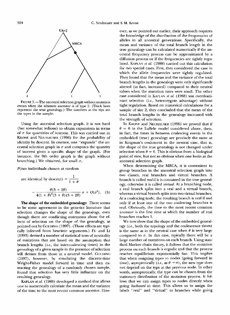
Figures 4 and 5 show realizations of the ancestral selection graph (displayed in Figure 1) with embedded true genealogies and sample outcome when assigning the two possible types to the ultimate ancestor. (In Fig- ures 4 and 5, a 1 stands for type AI and a 2 for type A*.) It should be clear from the graphs that the time to the MRCA depends on the type of the UA.

We can summarize our observations as follows. We obtain the ancestral selection graph in the selective case

1 2 2

FIGURE 4.-The ancestral selection graph without mutation events when the ultimate ancestor is of type 1. (Thick lines represent the true genealogy.) The numbers at the tips are the types in the sample.

with mutation by first selecting a graph according to the branching/coalescing process. We run this process until the first time its size is equal to 1. We then put mutation events along the branches according to the points of a Poisson process with rate 8/2, independently along each branch of the graph. Then, assigning the UA its type, we run the process forward in time and use Table 1 to see which branches are part of the true genealogical tree. We can then extract the true (embedded) genealogy.

We remark that the ancestral selection graph (more precisely, the true genealogical tree embedded in this graph) gives an approximation to the genealogical behavior of a sample from a Jinite population of size N. To do this, of course, it is necessary to interpret one unit of time in the ancestral selection graph as N / 2 units of time in the finite population model.

It is interesting to note that, at first glance, the ancestral selection graph looks like the graph one obtains in the case of recombination without selection (GRIFFITHS 1991; GRIFFITHS and MARJORAM 199’7); the way the graphs are interpreted, however, is very different in the two cases and there are basically no further similarities between the selection case and the neutral case with recombination.

The above algorithm for constructing the ancestral selection graph and extracting the embedded genealogy can be used to simulate samples. Since the state space is very large, this is not a very efficient way if one wishes to estimate the probability of a particular sample configuration. GRIFFITHS and TAV& (199413) developed a scheme using Markov chain Monte Carlo methods for approximating these sampling probabilities by simulating backward along the sample paths of the genealogy. In KRONE and NEUHAUSER (1996), we derive a recursion formula that can be used to carry out this simulation scheme.


UA=2

2 1 1

FIGURE 5.-The ancestral selection graph without mutation events when the ultimate ancestor is of type 2. (Thick lines represent the true genealogy.) The numbers at the tips are the types in the sample.

Using the ancestral selection graph, it is not hard (but somewhat tedious) to obtain expansions in terms of 0 for quantities of interest. This was carried out in KRONE and NEUHAUSER (1996) for the probability of identity by descent. In essence, one “expands” the ancestral selection graph in D and computes the quantity of interest given a specific shape of the graph. (For instance, the 0th order graph is the graph without branching.) We obtained, for small n,

P(two individuals chosen at random

1 are identical by descent) = -

1 + e

d(5 + 28) - q 1 + e)*(3 + e)(3 + 20)

ff + O(a2). (5)

The shape of the embedded genealogy: There seems to be some agreement in the genetics literature that selection changes the shape of the genealogy, even though there are conflicting statements about the effects of selection on the shape of the genealogy, as pointed out by GOLDINC (1997). (These effects are typically inferred from heuristic arguments.) FU and LI (1993) devised a number of statistical tests of neutrality of mutations that are based on the assumption that branch lengths ( i e . , the intercoalescing times) in the genealogy of a given sample in the presence of selection will deviate from those in a neutral model. GOLDINC (1997), however, by simulating the discrete-time Wright-Fisher model forward in time and then extracting the genealogy of a randomly chosen sample, found that selection has very little influence on the resulting genealogy. -LAN et al. (1988) developed a method that allows

one to numerically calculate the mean and the variance of the time to the most recent common ancestor. How-

ever, as we pointed out earlier, their approach requires the knowledge of the distribution of the frequencies of alleles in all ancestral generations. Specifically, the mean and variance of the total branch length in the true genealogy can be calculated numerically if the ancestral frequency process can be approximated by a diffusion process or if the frequencies are tightly regulated. -LAN et al. (1988) carried out this calculation for two special cases. First, they considered the case in which the allele frequencies were tightly regulated. They found that the mean and the variance of the total branch lengths in the genealogy were only significantly altered (in fact, increased) compared to their neutral values when the mutation rates were small. The other case considered in KAPLAN et al. (1988) was overdomi- nant selection ( i . e . , heterozygote advantage) without tight regulation. Based on numerical calculations for a sample of size 2, they concluded that the mean of the total branch lengths in the genealogy increased with the strength of selection.

In KRONE and NEUHAUSER (1996) we proved that if 0 = 0 in the 2-allele model considered above, then, in fact, the times in between coalescing events in the embedded (true) genealogy are precisely the same as in Kingman’s coalescent in the neutral case, that is, the shape of the true genealogy is not changed under selection when 0 = 0. This is obvious from a biological point of view, but not so obvious when one looks at the ancestral selection graph.

When determining the MRCA, it is convenient to group branches in the ancestral selection graph into two classes, real branches and virtual branches. A branch is called real if it is contained in the true genealogy, otherwise it is called virtual. At a branching node, a real branch splits into a real and a virtual branch, whereas a virtual branch splits into two virtual branches. At a coalescing node, the resulting branch is real if and only if at least one of the two coalescing branches is real. Obviously, the time to the most recent common ancestor is the first time at which the number of real branches reaches 1.

We now show that the shape of the embedded genealogy (i.e., both the topology and the coalescence times) is the same as in the neutral case when 8 is very large compared to u. In this case, typically there will be a large number of mutations on each branch. Using standard Markov chain theory, it follows that the mutation process on each branch is ergodic and that the process reaches equilibrium exponentially fast. This implies that when assigning types to nodes (going forward in time), asymptotically ( i e . , as 0 -+ m), the new type does not depend on the type at the previous node. In other words, asymptotically, the type can be chosen from the stationary distribution of the mutation process. It follows that we can assign types to nodes directly when going backward in time. This allows us to assign the labels “real” and “virtual” to branches while going


backward in time. Using the appropriate table, we can find the embedded genealogy without knowledge of the type of the ultimate ancestor. Since pairs of real branches coalesce at rate (;) if k real branches are present, it follows, as in the case 8 = 0, that the coalescence times are asymptotically the same as in the neutral case. The above argument can be applied to the case when the mutation process is asymmetric, as long as both mutation rates are large compared to a.

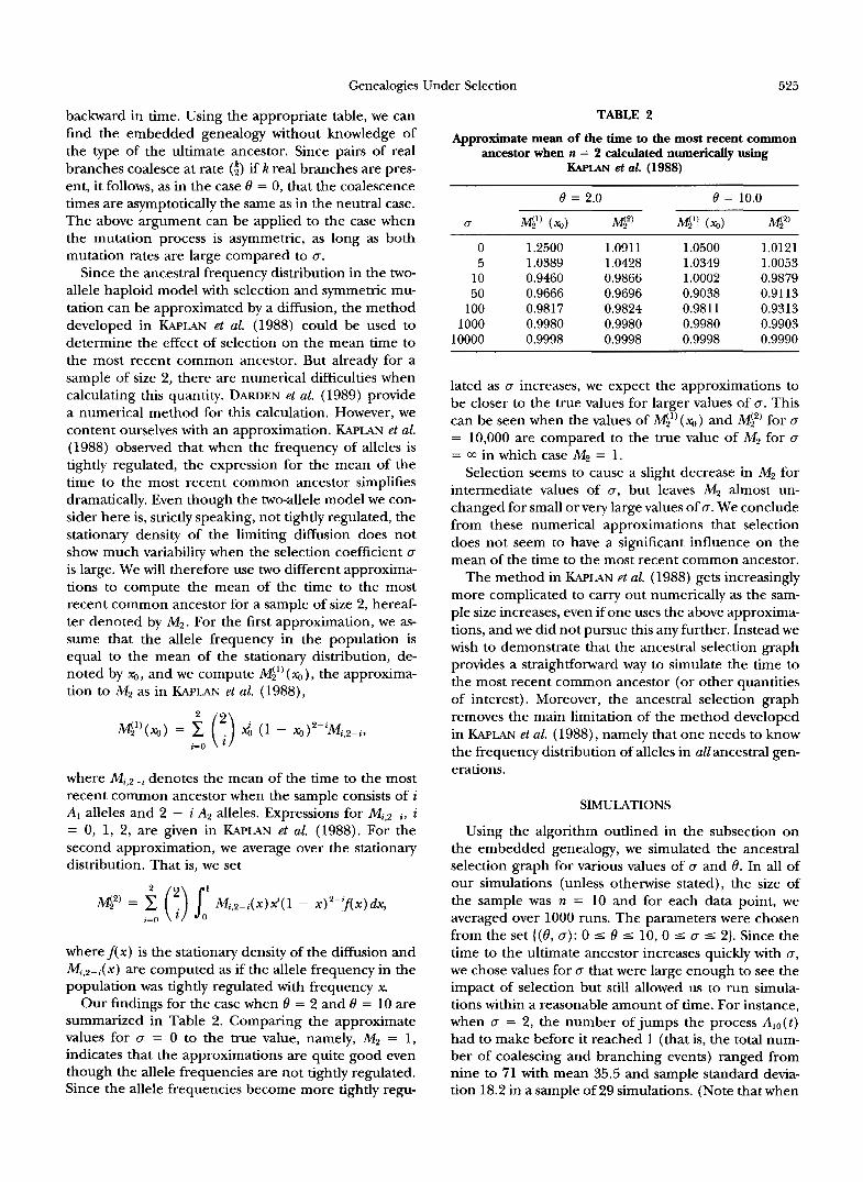
Since the ancestral frequency distribution in the two- allele haploid model with selection and symmetric mutation can be approximated by a diffusion, the method developed in KAPLAN et al. (1988) could be used to determine the effect of selection on the mean time to the most recent common ancestor. But already for a sample of size 2, there are numerical difficulties when calculating this quantity. DARDEN et al. (1989) provide a numerical method for this calculation. However, we content ourselves with an approximation. KAPLAN et al. (1988) observed that when the frequency of alleles is tightly regulated, the expression for the mean of the time to the most recent common ancestor simplifies dramatically. Even though the two-allele model we consider here is, strictly speaking, not tightly regulated, the stationary density of the limiting diffusion does not show much variability when the selection coefficient a is large. We will therefore use two different approximations to compute the mean of the time to the most recent common ancestor for a sample of size 2, hereaf- ter denoted by M2. For the first approximation, we assume that the allele frequency in the population is equal to the mean of the stationary distribution, denoted by %, and we compute “21’ (%), the approximation to M2 as in KAPLAN et al. (1988),

where Mj,2-i denotes the mean of the time to the most recent common ancestor when the sample consists of i AI alleles and 2 - i A2 alleles. Expressions for Mi,2-i, i = 0, 1, 2, are given in KAFTAN et al. (1988). For the second approximation, we average over the stationary distribution. That is, we set

where f i x ) is the stationary density of the diffusion and Mi,2- i ( x) are computed as if the allele frequency in the population was tightly regulated with frequency x.

Our findings for the case when 8 = 2 and 8 = 10 are summarized in Table 2. Comparing the approximate values for a = 0 to the true value, namely, M2 = 1, indicates that the approximations are quite good even though the allele frequencies are not tightly regulated. Since the allele frequencies become more tightly regu-

TABLE 2

Approximate mean of the time to the most recent common ancestor when n = 2 calculated numerically using

KAPLAN et al. (1988)

0 = 2.0 0 = 10.0

U “21’ (Go) “21’ (xa) M!’ 0 1.2500 1.0911 1.0500 1.0121 5 1.0389 1.0428 1.0349 1.0053

10 0.9460 0.9866 1.0002 0.9879 50 0.9666 0.9696 0.9038 0.9113

100 0.9817 0.9824 0.981 1 0.9313 1000 0.9980 0.9980 0.9980 0.9903

10000 0.9998 0.9998 0.9998 0.9990

lated as a increases, we expect the approximations to be closer to the true values for larger values of a. This can be seen when the values of (% ) and 11.1‘22’ for (T

= 10,000 are compared to the true value of M2 for a = m in which case M2 = 1.

Selection seems to cause a slight decrease in M2 for intermediate values of a, but leaves M2 almost unchanged for small or very large values of a. We conclude from these numerical approximations that selection does not seem to have a significant influence on the mean of the time to the most recent common ancestor.

The method in KAPLAN et al. (1988) gets increasingly more complicated to carry out numerically as the sample size increases, even if one uses the above approximations, and we did not pursue this any further. Instead we wish to demonstrate that the ancestral selection graph provides a straightforward way to simulate the time to the most recent common ancestor (or other quantities of interest). Moreover, the ancestral selection graph removes the main limitation of the method developed in KAPLAN et al. (1988), namely that one needs to know the frequency distribution of alleles in allancestral generations.

SIMULATIONS

Using the algorithm outlined in the subsection on the embedded genealogy, we simulated the ancestral selection graph for various values of a and 8. In all of our simulations (unless otherwise stated), the size of the sample was n = 10 and for each data point, we averaged over 1000 runs. The parameters were chosen from the set ( (8 , a): 0 5 8 I 10, 0 5 a 5 2). Since the time to the ultimate ancestor increases quickly with a, we chose values for (T that were large enough to see the impact of selection but still allowed us to run simulations within a reasonable amount of time. For instance, when o = 2, the number of jumps the process A, , ( t ) had to make before it reached 1 (that is, the total number of coalescing and branching events) ranged from nine to 71 with mean 35.5 and sample standard devia- tion 18.2 in a sample of 29 simulations. (Note that when


theta = 1.0

sigma

o = 0, the number of steps is always n - 1; that is, nine for our choice of parameters.) The value o = 2 is already large enough to see the effect of selection on the allele frequencies. If p1 (a , 0) denotes the expected frequency of the Al-allele in equilibrium, then p1(2 , 0.1) = 0.1656, p1(2, 1.0) = 0.3435 and p 1 ( 2 , 10.0) = 0.4762.

We used simulations to address the question of whether TMRcA depends on o for given 8. For 0 fixed, we varied o from 0 to 2. Based on our theoretical observations above, we do not expect T M R , to depend on o when 0 = 0 or 0 P c, This was in fact observed when 8 = 0 and 8 = 10. A linear regression analysis was performed in each case and no statistically significant de- pendence of T M R , on o was detected in either case. Furthermore, in each case, the data points are clustered around 1.8, the expected value under neutrality.

Intermediate values of 8 do not give such a clear picture. We performed simulations for 0 = 1 and o varying from 0 to 2. The results are summarized in Figure 6. A linear regression analysis showed a statistically significant decrease in TMR, as o increased. How- ever, this decrease is fairly small. In addition, we tested the hypothesis that both samples were drawn from the same distribution. For 8 = 1, we simulated 30 runs for a = 0 and for o = 2. We ranked the data and computed the Wilcoxon statistic. We did not find a statistically significant difference in the two samples ( P = 0.3844). This behavior was observed in other simulations as well. Typically, a statistically significant decrease of TMRcA occurred but the hypothesis of both samples being from the same distribution could not be refuted.

Since the embedded (true) genealogy has a coalescing structure, we can simulate the coalescing times in the embedded genealogy. We employed the Kolmo-

FIGURE 6.-TMRc;A us. a for H = 1.0. The linear regression equation is 1.82 - 0 .049~ and the correlation coefficient r = -0.76. The corresponding Fsta- tistic is F = 31.16, which is significant (F".,,,,,,, = 9.07, P < 0.010). (The dots are simulation results, the solid line is the regression curve.)

gorov-Smirnov test to see whether these times deviate from the corresponding expected distribution under neutrality. Under neutrality, the time it takes to reduce the number of ancestors from k to k - 1, is exponentially distributed with parameter (i). For n = 10 and 0 = 1, the Kolmogorov-Smirnov statistics, Dloo( k ) , k = 2, 3, . . . , 10, were computed for each of T,, T? , . . . , TI(,, based on 100 simulations for each of o = 0 and o = 2. The maximum values for 10 different runs are reported in Table 3. We were not able to detect a statistically significant change in the distribution of coalescing times.

Our conclusion, based on simulations and the numerical computation of the mean of the time to the MRCA of a sample of size 2 using the method in -LAN

et al. (1988), is that the shape of the embedded genealogy for the two-allele haploid model with selection and symmetric mutation does not change considerably under selection. It appears that intermediate values of o decrease branch lengths slightly, but for small or very large values of o (compared to e), the branch lengths are essentially unchanged compared to their neutral values. Incidentally, a similar observation of a slight de-

TABLE 3

Omax = mak=2,3 , . . . ,10 DIOO (k)

a = o L7 = 2"

0.034 0.055 0.061 0.085 0.057 0.056 0.033 0.077 0.035 0.042 0.052 0.083 0.056 0.048 0.079 0.043 0.037 0.060 0.049 0.048

Genealogies Under Selection 52’7

crease of branch lengths was made by GOLDING (1997), but he also remarked that the effect of selection on branch lengths is minor. When c is very large, almost all individuals in the population are of the advantageous type and hence comparatively neutral. It should therefore not be too surprising that the branch lengths are indistinguishable from their neutral values. In other words, at branching points, most of the time the incoming branch is contained in the true genealogy and a similar argument as for the case when 0 = 0 should hold.

Even though the shape of the embedded genealogy is similar to that of the neutral coalescent (and in some cases the shape is actually the same), this does not mean that one can simply use the coalescent to simulate the ancestry of a sample when selection is present. When extracting the embedded genealogy from the ancestral selection graph, one uses certain rules at branching nodes to decide which path to take. Even though these branching nodes are no longer visible in the embedded genealogy, they introduce a bias toward the advantageous type. One can therefore use the coalescent to simulate genealogies under selection only if one knows the distribution of the frequencies of alleles in all ancestral generations. [This was exploited in KAPLAN et al. (1988).] The ancestral selection graph allows one to simulate the genealogy of a sample without knowing the frequencies of alleles at all ancestral times; one only needs to know the type of the ultimate ancestor to obtain a sample together with its genealogy.

The ancestral selection graph can also be used to simulate allele frequencies at stationarity by simulating large samples iteratively in the following way. In the first step of the iteration, one starts with a particular type for the ultimate ancestor and obtains a sample distribution for the allele frequencies. Using this frequency distribution for choosing the ultimate ancestor in the next iteration, one obtains a (possibly) different frequency distribution. Repeating this until the frequency distribution stabilizes gives the stationary distribution.

We wish to point out that the above results apply to the limiting case of an infinite population that evolves according to the described dynamics. When the population is finite, there is positive probability that a branching event coincides with a coalescing event (simply when the 2-arrow causing the branching connects two branches that are already in the ancestral graph). This presumably causes a decrease in the coalescing times. As was mentioned earlier, the shape of the embedded genealogy can change substantially under different selection schemes (see KAPLAN et al. 1988). That is, our conclusions only apply to the particular model we used. The point we wish to make, however, is that one should proceed with caution when using statistical tests based on the assumption that branch lengths change when selection is present, such as in the test of

Fu and LI (1993). Such tests will detect deviations from neutrality only in cases where selection substantially changes the shape of the (true) ancestral tree.

OTHER MODELS

In this section, we present a number of models for which the ancestral selection graph and the embedded genealogy can be obtained. All these models necessarily have in common that there are only finitely many selection classes. The analysis of these more complicated models is very similar to that of the above symmetric 2- allele model. We present these models as versions of the continuous-time Moran model since that is the most natural setting for constructing the ancestral selection graph. However, we remind the reader that all of this works just as well for discrete-time models like Wright- Fisher. As long as the diffusion limit is the same as that of a given Moran model, the ancestral selection graphs will also be the same. The other aspect that is the same for the models below is the relative ease with which one can simulate samples and the associated genealogy. Just as for the neutral coalescent, this approach is much more efficient than simulating a large population forward in time and then extracting a sample. The genealogical approach has the advantage of keeping track only of the lines of descent that influence the sample.

The &allele model: Here, we again have a haploid population of Nindividuals evolving according to a continuous-time Moran model, but this time we allow the gene under consideration to have K 2 2 alleles, AI , . . . , AK, with respective reproduction parameters A, 5 A2 5 * - - 5 XK. For example, the gene might refer to a single site on a chromosome and the alleles could be the four nucleotides A, C, G, and T. Or, the gene might refer to a codon, thus having 43 = 64 alleles. The probability that the offspring of an individual of type A, is a mutant is denoted by pN(i), i = 1,2, . . . , K, and given that the offspring is a mutant, a mutation from type Ai to type Ai occurs with probability yi j . This defines a K X K transition matrix r = (y i j ) ls , , j sK. That is, an individual of type Ai gives birth to a new individual at rate X i and the type of the offspring will be Ajwith probability pN( i )yv . Notice that, unlike the previous model, this model allows for mutation probabilities that are not symmetric and depend on the type of the parent.

We set

Xi = A I ( 1 + sN(i)), i = 2, 3, . . . , K, (6)

with 0 5 sN( 2) 5 sN(3) 5 * * * 5 sN( K ) . With the scaling XI = N/2, NpN( i) = B i , and NsN( i) = cj, the genealogical process converges, as N - r 03, to a coalescing, branching graph similar to the one in the previous model. If K z 3, however, each incoming branch must have a label in {2, . . . , K ) that determines the types that can proceed through the branch forward in time. To explain this, let us call an incoming branch with label i, for i = 2,


TABLE 4

Rules at branching points for three-allele model


1 1 1 N 1 2 2 N 1 3 3 N 2 1 2 Y 2 2 2 Y 2 3 2 Y 3 1 3 Y 3 2 3 Y 3 3 3 Y

Branch labeled I is the type-2 incoming branch.

. . . , K, a type-i incoming brunch, and the corresponding branching point a type-i brunching point. The ancestral selection graph begins with n ancestors and, as time recedes into the past, the number of ancestors goes up and down by jumps of size 1 due to branching and coalescing. If there are currently k ancestors (going backward in time), we get coalescing at rate (i) and branching at an overall rate of kaK/2. More specifically, we get type-2 branching points at rate k(X, - X,) = ka2/2, type-3 branching points at rate k(X, - X,) = k(a3 - a2)/2, . . . , and type-K branching points at rate k(XK

- AK-l) = k ( a K - aK-1)/2. Note that 0 s a2 5 - - 5 aK < m. In general, a type-i incoming branch allows individuals with type AI to pass through the corresponding branching point (forward in time) if and only if j 2 i. If this happens, the type that emerges (forward in time) through the branch point will be AI and the incoming branch will be a part of the true genealogical tree. The continuing branch (i.e., the other branch running into the branching point) is then not a part of the true genealogy and it is removed as in the 2-allele case. On the other hand, if the type entering the branching point on the incoming branch is not allowed to pass through the branching point (i.e., if j < i), then the type on the continuing branch is the one that passes through. In this case, the incoming branch will not be part of the true genealogical tree and is removed. Note

TABLE 5

Rules at branching points for three-allele model


1 1 1 N 1 2 2 N 1 3 3 N 2 1 1 N 2 2 2 N 2 3 3 N 3 1 3 Y 3 2 3 Y 3 3 3 Y

Branch labeled I is the type-3 incoming branch.

I 11


that the selectively inferior Al individuals can never pass through a branching point from an incoming branch.

Once the ancestral selection graph is constructed, we can superimpose the mutation process on the graph as in the previous model. Mutations affecting type A, individuals occur at rate OJ2 along the branches, and the types are then chosen according to the transition matrix r defined above. In other words, mutations Ai -+ Aj occur at rate O,y,/2 along the branches of the ancestral graph. (Mutations for type A, individuals have no effect on individuals not of type A; . )

Again, the ultimate ancestor will appear in finite time. (Equations 3 and 4 hold with aK in place of a.) To determine the sample and the true genealogical tree, we start the UA with its type and run the process forward in time, as before. A look-up table similar to Table 1 tells us what happens when we pass through branching points. The look-up tables for the case of K = 3 are shown in Tables 4 and 5. Since there are two different selection coefficients, we need two tables; one for the case where the incoming branch is labeled with a 2, and one for the case where the incoming branch is labeled with a 3. The graphs accompanying Tables 4 and 5 are in Figures 7 and 8, respectively. We put the label near the end of the incoming branch (i.e., near the branching point) because it is only the type that

I I1


Genealogies I

tries to pass through the branching point (forward in time) that matters. It follows from Tables 4 and 5 that the incoming branch is kept if and only if the type entering the branching point through a type-iincoming branch is zi. Note that the types along the incoming branch can change via mutation in any way allowed by the mutation process. However, only the type that tries to cross the branching point is important for determing which type emerges from the branching point (forward in time) and whether the incoming branch is actually used in the true genealogical tree.

The infinitely-many-alleles model: Having defined the ancestral selection graph for a K-allele model, we can extend this immediately to infinitely-many-alleles models with d selection classes. This class of models was introduced in ETHIER and KURTZ (1987, 1994); see also JOYCE and TAV& (1995) for an application. In these models, each gene is assigned a type x E [0, 1). Alleles are grouped into d z 2 classes ( d finite), and the selection coefficients are constant for alleles in a given class. To do this, we define ~0 = 0, cd = 1 and numbers cI < g < * < cdPl E (0, 1) and set

We say that an allele of type x E [0, 1) falls into the jth selection class if x E 4. The reproduction rate of an individual in the jth selection class is then defined as

with 0 I sN( 1) 5 sN(2) 5 - - 5 sN( d ) . The population evolves according to a Moran model. When a reproduction occurs, the type of the offspring is chosen according to the mutation process; that is, the offspring is either of the same type as the parent if no mutation occurs, or of a type that has not been previously observed in the population. This can be done by choosing a number x E [0, 1) according to some continuous distribution. The value x will denote the new mutant type (which will be different from all previous types with probability 1) and the selection class is determined by the interval into which xfalls. One can then proceed as in the K-allele case. The ancestral selection graph again has the same coalescing, branching structure. To get the true ancestral tree, assign the UA its type and run the process forward in time using look-up tables similar to Tables 4 and 5.

DNA sequence models: Here, the type space for a gene is E = {A, C, G, T)M; i.e., sequences of length M, each element of which is one of the four nucleotides A, C, G, or T. Of course, different alphabets could also be used, depending on the application. For example, if one is interested in regions where transversions are not allowed, a binary alphabet would be appropriate. Another possibility is to use a 20-letter alphabet to model the different amino acids that can occur in a protein. In this case, a “site” in the corresponding DNA

Jnder Selection 529

sequence would refer to a codon. Let us consider the case where certain sequences are classified as (slightly) deleterious and the rest are classified as neutral. In light of recent data on DNA polymorphism ($ BROWN and CLEGG 1983; KREITMAN 1983), this is a natural model. For example, one could model the case where nucleotide substitutions resulting in amino acid changes are deleterious [$ KREITMAN’S (1983) data that suggests this type of selection for the Adh locus of Drosophila mlanogaster]. We will only give details for the case where there is only one deleterious class ( i e . , two selection classes), although this is easily extended to more than two selection classes, as we did in the K-allele model and as we will do for the infinite-sites model, below. We thus have a decomposition of the type space as a disjoint union, E = El U I$, where El denotes the deleterious sequences and denotes the neutral sequences. Sup- pose the population size is N. To model deleterious mutations, let us change our notation a bit and assume that a neutral individual reproduces at rate )b, and an individual with deleterious type reproduces at rate XI = )b(l - s N ) , 0 I sN < 1. At the time of a reproduction event, an individual is chosen at random from the population to die. The type of the new individual is the same as its parent with probability 1 - uN and is of a mutant type with probability uN. Given that a mutation occurs in the new individual, a site is selected at random from some distribution f = ( f i , . . . , fM), with f i + - - - + fM = 1. Note that this allows us to model “hot spots” for mutation along the sequence. If site 1 is chosen to mutate, then the nucleotide at this site is changed according to the lth mutation matrix rcO = (yb0); this is a 4 X 4 matrix giving the probabilities for one nucleotide changing to another. For example, given that a mutation occured, the transition

. . . (21,. . . 9 i M ) “f (21, . . . 9 Z l P l > j , k + l , . . . 9 iM)

will occur with probability fivl,“,. Note the implicit assumption that the type of the mutant nucleotide depends only on the nucleotide at the site being mutated and not on what is at nearby sites. Notice that by allowing a nucleotide to “mutate” to itself with positive probability, we can get some nucleotides mutating more slowly than others. [ Cf: BROWN and CLEGG (1983) for an example where nucleotides C and G mutate much faster than nucleotides A and T. HARTL and CLARK (pp. 115-1 16,1989) give a summary of this data.) Of course, a mutation will sometimes change the fitness of the new individual.

If we now consider the genealogy of a sample of size n from such a population with parameters scaled in the usual way ( i .e . , X. = N/2, NsN = u and NuN = e ) , then as N -+ cc we get the same ancestral selection graph structure as before; the structure of the mutation process does not affect this. Therefore, going back in time, if there are currently k ancestors in the graph, then coalescing takes place at rate (;) and branching takes


place at rate b / 2 . On the branches of the ancestral selection graph we lay down mutations according to Poisson processes that are independent on different branches. The overall mutation rate on a given branch is 8/2; the site of a mutation is chosen according to the distribution f and, once the site is chosen, the type of mutation is determined according to the appropriate mutation matrix. In other words, along each branch of the ancestral selection graph, there are mutations at site 1 from allele Ai to allele Ai at rate (B/2)flyh0. When going forward in time along a branch, such a mutation will be ignored if the individual does not have allele Ai at site 1. The form of the mutations only matters in determining which branches are actually used in the true ancestral tree (and this only depends on the selective classes of the individuals going forward in time) and, of course, in determining the actual types (DNA sequences) of the n individuals in the sample.

We remark that it is easy to alter the above model to include more than two selective classes, possibly with advantageous alleles as well. Furthermore, one can allow for a Poisson number of mutations during a reproduction event, rather than just one. We will do this for the infinite-sites model in the next section; the necessary changes for this model should then be clear.

The infinitely-many-sites model: The neutral infinite sites model was introduced by WATTERSON (1975). Such models are meant to approximate certain features of a long DNA sequence. The idea is that if the mutation rate per site is very small, then back mutations will be very rare. The infinitely-many-sites model does not allow back mutations, thus simplifying the analysis. To sim- plify things still further, one only keeps track of which sites have experienced a mutation since the MRCA of a sample; the actual type mutated to (e.g. , nucleotide substitution) is not considered. The resulting model is in some ways much more tractable than more explicit models of DNA sequences.

Suppose we have a population of size N. With the above assumptions in mind, it is natural to model the region of interest as the interval [0 , 11. For each new individual, a Poisson number of sites is chosen to mutate. Each such site is selected independently according to a density functionfconcentrated on [0,1]. For example, if is the mean for the above Poisson distribution, then given there is a reproduction event, there will be mutations at k sites located in the intervals [xl , x1 +

approximately dX, ] , [Q, % + d Q ] , . . . , [Xk, X k + d X k ] with probability

k - uN

t? "J"-f(Xl)f(Q) ' ' f ( X k ) d X l d Q ' ' * dxk. k!

It follows that all mutations will be at new sites (no back mutations). The shape off determines whether there are mutational hot spots or cold spots. A Poisson distribution for the number of sites that experience mutation during a given reproduction event is natural in light of

the assumptions of small mutation probability per site and a large number of sites. Note that the probability, uN, that there is at least one mutation is

uN = 1 - e-"X

per reproduction event per individual. The probability of getting k 2 1 new mutant sites, given that at least one mutation occurred, is

We now add selection to the model by assuming that there are parts of the interval (sequence) at which a mutation would have a deleterious effect. Mutations at other sites in the interval are considered to be neutral. Let us assume that the fitness of an individual depends only on the number of deleterious mutations it has and not on the actual types of the mutations. Neutral individuals reproduce at rate Xo. Individuals with k 5 d deleterious mutations reproduce at rate kk = &,(I - sAV( k ) ) , where 0 5 sN( 1) 5 sZV(2) 5 * - * 5 sN( d ) < 1. In addition, we assume that individuals with more than d deleterious mutations reproduce at rate X d = X,( 1 - sN( d ) ) . Thus, we have d + 1 selection classes (including neutral individuals).

Next, scale the parameters in the obvious way: X, = N/2, uaV = B/N, sAT(k) = ak /N , where 0 5 u1 a2 -= - * 5 ad < m. Note that the mean number of sites that mutate in a reproduction event is -

vhr = -ln(l - B/N) - B/N,

for large N. It follows that

(1 - B/N)(B/N)k" ~

qN(k ) k! 0 i f k z 2 ,

as N+ a. In other words, in the limiting object, we get exactly one site mutated per mutation event. So, taking N+ 00, we can describe the genealogy of a sample of n individuals with the resulting ancestral selection graph, whose structure should by now be apparent. When there are k ancestors, we get coalescing at rate ( 4 ) and, for i = 1, . . . , d - 1, we get type-i branches at rate k ( X j - Ai+,) = k(a,+l - a, ) /2 , and we get type-0 branch points at rate k(Xo - X,) = b J 2 , yielding an overall branching rate of k5$2. Only individuals with 5 i deleterious mutations can pass through a type-i branch point (forward in time) along an incoming branch. Once the ancestral selection graph has been constructed, we lay mutations along the branches in the usual way, at rate 8/2. At the time of such a mutation, the type of an individual changes by adding a single new mutant site according to the probability density6

To determine the types of the sample and the true genealogical tree, we proceed as before, starting the UA with its type and running the process forward in


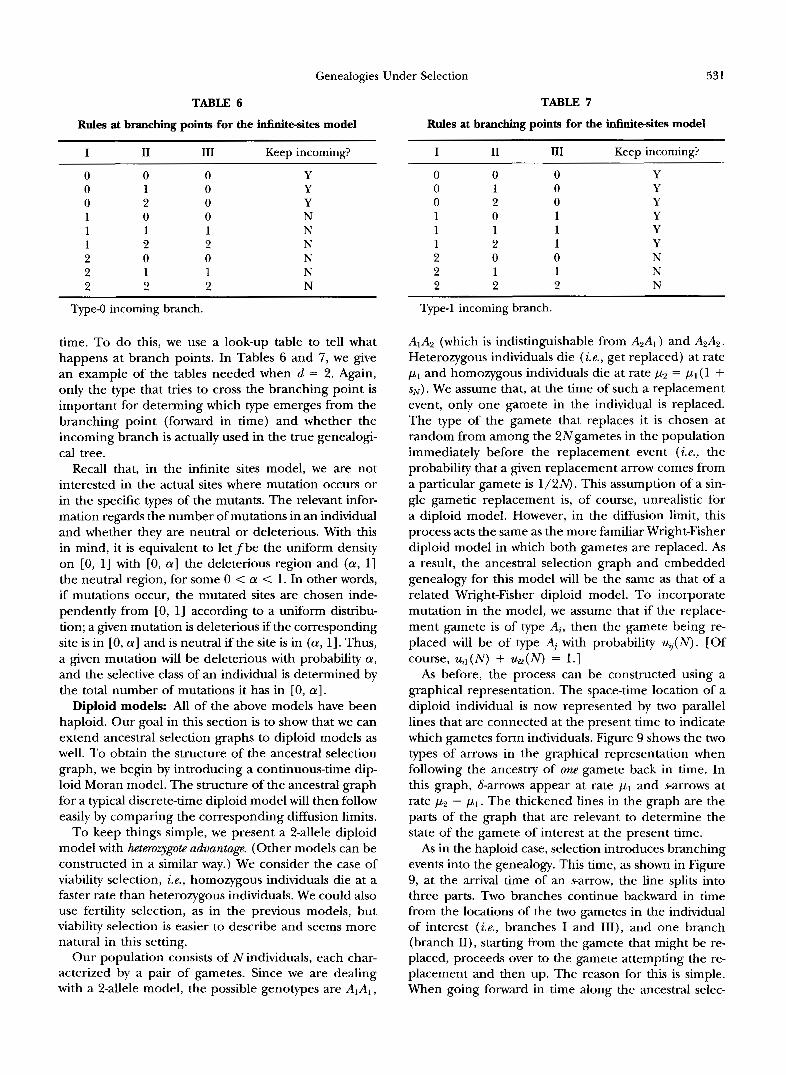
TABLE 6 Rules at branching points for the infinitesites model


0 0 0 Y 0 1 0 Y 0 2 0 Y 1 0 0 N 1 1 1 N 1 2 2 N 2 0 0 N 2 1 1 N 2 2 2 N

Type4 incoming branch.

time. To do this, we use a look-up table to tell what happens at branch points. In Tables 6 and 7, we give an example of the tables needed when d = 2. Again, only the type that tries to cross the branching point is important for determing which type emerges from the branching point (forward in time) and whether the incoming branch is actually used in the true genealogical tree.

Recall that, in the infinite sites model, we are not interested in the actual sites where mutation occurs or in the specific types of the mutants. The relevant information regards the number of mutations in an individual and whether they are neutral or deleterious. With this in mind, it is equivalent to letfbe the uniform density on [0, 11 with [0, a ] the deleterious region and (a, 11 the neutral region, for some 0 < a < 1. In other words, if mutations occur, the mutated sites are chosen independently from [0, 13 according to a uniform distribution; a given mutation is deleterious if the corresponding site is in [0, a ] and is neutral if the site is in (a, 11. Thus, a given mutation will be deleterious with probability a, and the selective class of an individual is determined by the total number of mutations it has in [0, a ] .

Diploid models: All of the above models have been haploid. Our goal in this section is to show that we can extend ancestral selection graphs to diploid models as well. To obtain the structure of the ancestral selection graph, we begin by introducing a continuous-time d i p loid Moran model. The structure of the ancestral graph for a typical discrete-time diploid model will then follow easily by comparing the corresponding diffusion limits.

To keep things simple, we present a 2-allele diploid model with heterozygote advantage. (Other models can be constructed in a similar way.) We consider the case of viability selection, i.e., homozygous individuals die at a faster rate than heterozygous individuals. We could also use fertility selection, as in the previous models, but viability selection is easier to describe and seems more natural in this setting.

Our population consists of Nindividuals, each characterized by a pair of gametes. Since we are dealing with a 2-allele model, the possible genotypes are AIAI,

TABLE 7 Rules at branching points for the infinite-sites model


0 0 0 Y 0 1 0 Y 0 2 0 Y 1 0 1 Y 1 1 1 Y 1 2 1 Y 2 0 0 N 2 1 1 N 2 2 2 N

Type-1 incoming branch.

A1A2 (which is indistinguishable from A2A1) and A2A2. Heterozygous individuals die (i .e. , get replaced) at rate pl and homozygous individuals die at rate ~2 = ~ 1 ( 1 + sN) . We assume that, at the time of such a replacement event, only one gamete in the individual is replaced. The type of the gamete that replaces it is chosen at random from among the 2Ngametes in the population immediately before the replacement event ( i e . , the probability that a given replacement arrow comes from a particular gamete is 1/2N). This assumption of a single gametic replacement is, of course, unrealistic for a diploid model. However, in the diffusion limit, this process acts the same as the more familiar Wright-Fisher diploid model in which both gametes are replaced. As a result, the ancestral selection graph and embedded genealogy for this model will be the same as that of a related Wright-Fisher diploid model. To incorporate mutation in the model, we assume that if the replacement gamete is of type Ai, then the gamete being replaced will be of type AI with probability u,(N). [Of course, utl ( N ) + ut2(N) = 1.1

As before, the process can be constructed using a graphical representation. The space-time location of a diploid individual is now represented by two parallel lines that are connected at the present time to indicate which gametes form individuals. Figure 9 shows the two types of arrows in the graphical representation when following the ancestry of one gamete back in time. In this graph, &arrows appear at rate p l and parrows at rate pup - pl . The thickened lines in the graph are the parts of the graph that are relevant to determine the state of the gamete of interest at the present time.

As in the haploid case, selection introduces branching events into the genealogy. This time, as shown in Figure 9, at the arrival time of an sarrow, the line splits into three parts. Two branches continue backward in time from the locations of the two gametes in the individual of interest ( k . , branches I and 111), and one branch (branch 11), starting from the gamete that might be replaced, proceeds over to the gamete attempting the replacement and then up. The reason for this is simple. When going forward in time along the ancestral selec-


I11

I I I I I I I I I I I I I I I

FIGURE 9.-The graphical representation for the diploid model with viability selection in the case of heterozygote advantage. See text for explanation.

tion graph, we must know the genotype of the individual who receives the incoming branch at a branching point. (For example, a homozygous individual always “accepts” the incoming branch.) This allows us to determine the gametic type that passes through the branching point as well as which branch to include in the embedded genealogy. Notice that if one of the new branches is already in the genealogy, there is no need to add it.

If we now use the scaling p1 = N, NsN = u, Nulz(N) = 012, and (N) = 021, and let N + m, the resulting diffusion process describing the proportion of Al gametes in the population has drift (0/2)x(1 - x) (1 - 2x) - (O12/2)x + (e2J2) (1 - x) and diffusion parameter x(1 - x) . This is the same as the diffusion approximation for the classical diploid Wright-Fisher model that has, for population size N, fitnesses wll = y2 = 1 - (u/2)/2N, w12 = 1, and mutation probabilities u12 =

(OlZ/2)/2N, ‘ k 1 = (02,/2)/2N [$ EWNs (1979)l. The ancestral selection graph describing the geneal-

ogy of this model as N+ 03 has the following structure. Start with a sample of n gametes. (We do not require both gametes of an individual to be in the sample.) The number of ancestors goes up and down by jumps of the following types. If there are currently k ancestor gametes (going backward in time), we get coalescing of two randomly chosen ancestors at rate (i) and branching at rate b / 2 . Branching is different in the diploid case. At the time of a branching event, one of the k ancestor gametes is chosen at random to split into three “ancestral branches,” as shown in Figure 9. It is not hard to see that, in the limiting graph, the two new

RGURE 10.-A realization of the ancestral selection graph for a sample of two gametes.

branches must always be added, i e . , they will not already be present in the genealogy (with probability one).

Figure 10 shows a realization of an ancestral selection graph for a sample of two gametes that need not be from the same individual. The branch with the label s corresponds to the branch associated with the parrow, that is, the 11-branch in Figure 9. The continuing branch corresponds to the branch labeled I in Figure 9, the third branch is the one labeled I11 in Figure 9. The rule at a branching point is that, if the types coming down branches I and I11 are the same ( ie . , the individual is homozygous), then the type coming down the I1 branch continues; otherwise, the type on the I branch continues.

Even though we now allow jumps of size 2 due to branching, the size of the ancestral selection graph still has linear growth and quadratic death rates and hence we will reach an ultimate ancestor in finite time. Muta- tion events Al + A2 (respectively, A2 + Al ) are laid down along the branches of the ancestral selection graph according to independent Poisson processes with rates 012/2 (respectively, 02J2). Assigning the ultimate ancestor its (gametic) type, we can now run the process forward in time, determining the types in the sample and the true genealogy, as before.

DISCUSSION

Statistical tests for detecting selection [such as the test by Fu and LI (1993)l or statistical quantities for nucleotide variation (such as the number of segregating sites) are frequently based on properties of the ancestral tree describing the genealogy of a random sample. The test by Fu and LI (1993) is designed to detect changes in the shape of the ancestral tree under selection; the number of segregating sites in a sample of genes is related to the total length of branches in the ancestral tree of the sample. It is therefore essential to


understand the properties of the ancestral tree not only under neutrality but also under selection.

The genealogical process for many simple genetic models under neutrality is Kingman's coalescent (KING MANN 1982a,b); its properties have been widely studied [see the review articles by TAVAR~ (1984) and by DON- NELLY and TAV& (1995) and references therein]. The genealogical process for a two-allele haploid Wright- Fisher (or Moran) model with selection has only been recently characterized in KRONE and NEUHAUSER (1996). The purpose of this investigation is to extend this characterization to other models with selection in both the haploid and the diploid case and to explore some of the properties of this ancestral process.

The genealogy of random samples from large populations that evolve according to various simple genetic models with selection are presented here. The genealogy is embedded in a branching-coalescing graph, called the ancestral selection graph. Simple look-up tables are used to extract the true ancestral tree from this graph. The true ancestral tree has a coalescing structure and interest focuses on how its distribution depends on the selection coefficient.

It is straightforward to simulate the ancestral selection graph and thus it is possible to sample from the distribution of quantities such as coalescing times or the total length of all branches in the true ancestral tree by simulating data from the ancestral process. So far, little is known rigorously about how the distribu- tions of these quantities change under selection.

KAPLAN et ul. (1988) developed a method that allows one to compute the mean and the variance of the total length of branches in the genealogy in cases where the ancestral frequency process can be approximated by a diffusion process or where the frequencies are tightly regulated. Their method, however, requires the knowledge of the distribution of allele frequencies in all ancestral generations. They found cases where selection substantially increases the total length of branches in the genealogy.

We investigated the two-allele haploid Moran model with selection and symmetric mutation and sampled from the distribution of coalescing times by simulating the corresponding ancestral selection graph. We found that the distribution does not change much under selection in this particular case. Simulations indicate that for values of the mutation rate that are comparable to the selection coefficient, the mean of the time to the most recent common ancestor decreases slightly. How- ever, this decrease was no longer statistically significant when we looked for differences in the distribution of the actual coalescing times. Furthermore, we proved rigorously that very small mutation rates or mutation rates that are very large compared to the selection coefficient yield the same distribution of the time to the most recent common ancestor as in the neutral case.

We only explored a small range of parameter values

for the selection coefficient since the size of the ancestral selection graph increases quickly with the selection coefficient. Our simulation results were substantiated by numerically approximating the time to the most recent common ancestor for a sample of size 2 using the method developed in KAPLAN et ul. (1988). The numerical a p proximations also allowed us to explore a wider range of parameter values for the selection coefficient.

The basic structure of the ancestral selection graph for other haploid models is essentially the same and we provide rules for other models that are important for practical applications. The branching mechanism is more complicated in the diploid case; we only discuss the case of heterozygote advantage with viability selection.

For very weak selection the ancestral selection graph can also be used to obtain polynomial approximations (in terms of a) for various quantities of interest. This is demonstrated in ONE and NEUHAUSER (1996) for the probability of identity by descent.

The models studied in this paper are mostly haploid. It is important to extend the analysis to diploid models and to include recombination. The ancestral selection graph allows one to explore alternative hypotheses for tests of neutrality that are based on properties of the ancestral tree; this enables one to assess the power of such tests.

C.N. is an Alfred P. Sloan Research Fellow and was partially sup ported by the National Science Foundation under grant DMS 9403644. This work was done while C.N. visited the Department of Ecology and Evolutionary Biology, Princeton University, during 1995/1996; she thanks the Department of Ecology and Evolutionary Biology at Princeton University for their warm hospitality. S.K. thanks HOLLY WICHMAN for discussions.

LITERATURE CITED

BROWN, A. H. D., and M. T. CLEGG, 1983 Analysis of variation in related DNA sequences, pp. 107-132 in StatisticalAnalysis ofDNA Sequence Data, edited by R. WEIR. Marcel Dekker, New York.

WNINGS, C., 1974 The latent roots of certain Markov chains aris-

Probab. 6: 260-290. ing in genetics: a new approach. I. Haploid models. Adv. Appl.

DARDEN, T., N. L. KAPLAN and R. R. HUDSON, 1989 A numerical method for calculating momentS of coalescent times in finite populations with selection. J. Math. Biology 27: 355-368.

DONNELLY, P., and S. TAV-, 1995 Coalescent and genealogical structure under neutrality. Annu. Rev. Genet. 2 9 401-421.

ETHIER, S. N., and T. G. KURTZ, 1987 The infinitely-many-alleles model with selection as a measure-valued diffusion. Lecture Notes in Biomaihematics 70: 72-86.

ETHIER, S. N., and T. G. KURTZ, 1994 Convergence to Fleming-Viot processes in the weak atomic topology. Stoch. Proc. Appl., 54:

EWENS, W. J., 1979 Mathematical Population Genetics. Springer, New York.

FISHER, R. A., 1930 The Genetical Theoly of Natural Selection. Clarendon Press, Oxford.

Fv, Y. X., and W. H. LI, 1993 Statistical tests of neutrality of mutations. Genetics, 133: 693-709.

GOLDING, G. B., 1997 The effect of purifying selection on genealogies, pp. 000-000 in Zh4.4 Volumes in Mathematics and its Applica- tions, vol. 87. Progress in Population Genetics and Human Evolution, edited by P. DONNELLY and S. TAV&. Springer, New York.

GRIFFITHS, R. C., 1991 The two-locus ancestral graph, pp. 100-117 in Selected Proceedings of the Symposium on Applied Probability, Shef-

1-27.


field, 1989, Vol. 18 of IMS Lecture Notes-Monograph Series. Institute of Mathematical Statistics.

G R I ~ S , R C., and P. MARJORAM, 1997 An ancestral recombination graph, pp. 000-000 in IMA Volum in Mathematics and its AppLiza- t i m , vol. 87. Progress in Population Genetics and Human Evolu- tion, edited by P. DONNELLY and S. TAVAR~. Springer, New York.

GRIFFITHS, R. C., and S. T A V ~ , 1994a Sampling theory for neutral alleles in a "y ing environment. Philos. Trans. R. SOC. London Ser. B 344: 403-410.

GRIFFITHS, R. C., and S. TAV&, 1994b Simulating probability distri- butions in the coalescent. Theor. Popul. Biol., 46: 131-159.

HAR~I., D., and A. CLARK, 1989 Princzples of Population Genetics. Si-

HUDSON, R. R., 1991 Gene genealogies and the coalescent process, nauer,

pp. 1-44 in Oxford Surueys in Evolutionaly Biology, edited by D. FUTWMA and J. ANTONOVICS. Oxford University Press, Oxford, UR

HUDSON, R R., and N. L. KAPLAN, 1988 The coalescent process in models with selection and recombination. Genetics 120 831-840.

JOYCE, P., and S. TAVAR~, 1995 The distribution of rare alleles. J. Math. Biol. 33: 602-618.

KAPLAN, N. L., T. DARDEN, and R. R. HUDSON, 1988 The coalescent process in models with selection. Genetics 120: 819-829.

KIMURA, M., 1956 Stochastic processes in population genetics, Ph.D. thesis. University of Wisconsin, Madison.

KINGMAN, J. F. C., 1982a The coalescent. Stoch. Proc. Appl., 13:

KINGMAN, J. F. C., 1982b On the genealogy of large populations. J. 235-248.

Appl. Prob., 19A 27-43.

KREITMAN, M., 1983 Nucleotide polymorphism at the alcohol dehy- drogenase locus of Drosophila melanogaster. Nature 304: 412-417.

KRONE, S., and C. NEUHAUSER, 1996 Ancestral processes with selection. Theor. Popul. Biol..

LUNDSTROM, R., S. TAV&, and R. WARD, 1992 Estimating mutation rates from molecular data using the coalescent. Proc. Natl. Acad. Sci. USA 8 9 5961-5965.

MOW, P. A. P., 1958 Random processes in genetics. Proc. Cam- bridge Phil. SOC. 5 4 60-71.

M O W , P. A. P., 1962 The Statistical Processes of Evolutionaly Theoly. Clarendon Press, Oxford.

SIMONSEN, R, G. CHUKCHII.I. and C. AQUADKO, 1995 Properties of statistical tests of neutrality for DNA polymorphism data. Genet- ics 141: 413-429.

SLATKIN, M., and W. MADDISON. 1989 A cladistic measure of gene flow inferred from the phylogenies of alleles. Genetics 123: 603-613.

TAJIMA, F., 1993 Statistical methods for testing the neutral mutation hypothesis by DNA polymorphism. Genetics 123: 585-595.

WATTERSON, G. A., 1975 On the number of segregating sites in genetical models without reC0mbindtiOn. Theor. Popul. Biol. 10:

WRIGHT, S., 1931 Evolution in Mendelian populations. Genetics 16:

WRIGHT, S., 1949 Adaptation and selection, pp. 365-389 in Genetics, Paleontology and Evolution, edited by G. L. JEPSON, G. G. SIMPSON and E. MAW. Princeton University Press, Princeton.

256-276.

97- 159.

Communicating editor: G. B. GOLDING

the genealogy of samples in models with selection · the genealogy of samples in models with...

Documents