THE EUROPEAN UNION BANANA MARKET: DEMAND ESTIMATION AND

EVALUATION OF THE NEW IMPORT REGIME

by

ADRIANA CHACÓN CASCANTE

Licenciada (B.A), Universidad de Costa Rica, 1998 MS, Kansas State University, 2004

AN ABSTRACT OF A DISSERTATION

submitted in partial fulfillment of the requirements for the degree

DOCTOR OF PHILOSOPHY

Department of Agricultural Economics

College of Agriculture

KANSAS STATE UNIVERSITY Manhattan, Kansas

2006

Abstract

The EU is one of the world’s biggest importers of bananas and, as such, import policies

enforced by this trade union are likely to have a great impact on major producers of bananas.

Aiming to protect communitarian producers and exporters from selected ex-colonies of Africa,

the Caribbean and Pacific and to honor previous agreements, the EU unified its import policy for

bananas in 1993. This policy, known as the Common Market Organization for Bananas,

generated one of the most controversial trade disputes in history. After several modifications of

the original regime, in January 2006, the EU changed its import regime to satisfy a World Trade

Organization mandate and to honor an agreement signed with the United States in 2000.

This dissertation reviews the history of the trade disputes in the EU banana market and

analyzes the effects that the new import regime will have on major suppliers. To do this, a

theoretically-consistent demand system is estimated and then the calculated parameters are used

to model the effects of the tariff-only import system in the EU banana market. Based on the

results, producers surplus are estimated and Monte Carlo simulations are performed to do a

sensitivity analysis of the results.

In the demand estimation component, the EU market is modeled as a system containing

four major suppliers using the Almost Ideal Demand System (AIDS). This estimation fills an

important gap in literature regarding the lack of well-estimated demand elasticities of bananas in

the EU.

The EU banana market is then modeled based on a equilibrium displacement model

framework. Results of this analysis are then used to calculate point estimates of producer surplus

changes as a measure of the impact of the new import policy on banana suppliers. Monte Carlo

simulations are based on parameter estimates obtained from the AIDS model. These simulations

allowed not only sensitivity analysis but also probabilistic inferences about the statistical

significance of the estimates obtained in the previous components.

Results indicate that the hypothesis that the new import regime will not affect the major

suppliers of the EU banana market cannot be rejected. This might indicate that the policy

enforced by the Common Market Organization for Bananas and the current tariff-only import

regime are statistically equivalent. In other words, the EU expertly enacted a tariff level that will

leave much as status quo.

THE EUROPEAN UNION BANANA MARKET: DEMAND ESTIMATION AND

EVALUATION OF THE NEW IMPORT REGIME

by

ADRIANA CHACÓN CASCANTE

Licenciada (B.A), Universidad de Costa Rica, 1998

MSc., Kansas State University, 2004

A DISSERTATION

submitted in partial fulfillment of the requirements for the degree

DOCTOR OF PHILOSOPHY

Department of Agricultural Economics

College of Agriculture

KANSAS STATE UNIVERSITY Manhattan, Kansas

2006

Approved by:

Major Professor John M. Crespi

Copyright

ADRIANA CHACÓN CASCANTE

2006

Abstract

The EU is one of the world’s biggest importers of bananas and, as such, import policies

enforced by this trade union are likely to have a great impact on major producers of bananas.

Aiming to protect communitarian producers and exporters from selected ex-colonies of Africa,

the Caribbean and Pacific and to honor previous agreements, the EU unified its import policy for

bananas in 1993. This policy, known as the Common Market Organization for Bananas,

generated one of the most controversial trade disputes in history. After several modifications of

the original regime, in January 2006, the EU changed its import regime to satisfy a World Trade

Organization mandate and to honor an agreement signed with the United States in 2000.

This dissertation reviews the history of the trade disputes in the EU banana market and

analyzes the effects that the new import regime will have on major suppliers. To do this, a

theoretically-consistent demand system is estimated and then the calculated parameters are used

to model the effects of the tariff-only import system in the EU banana market. Based on the

results, producers surplus are estimated and Monte Carlo simulations are performed to do a

sensitivity analysis of the results.

In the demand estimation component, the EU market is modeled as a system containing

four major suppliers using the Almost Ideal Demand System (AIDS). This estimation fills an

important gap in literature regarding the lack of well-estimated demand elasticities of bananas in

the EU.

The EU banana market is then modeled based on a equilibrium displacement model

framework. Results of this analysis are then used to calculate point estimates of producer surplus

changes as a measure of the impact of the new import policy on banana suppliers. Monte Carlo

simulations are based on parameter estimates obtained from the AIDS model. These simulations

allowed not only sensitivity analysis but also probabilistic inferences about the statistical

significance of the estimates obtained in the previous components.

Results indicate that the hypothesis that the new import regime will not affect the major

suppliers of the EU banana market cannot be rejected. This might indicate that the policy

enforced by the Common Market Organization for Bananas and the current tariff-only import

regime are statistically equivalent. In other words, the EU expertly enacted a tariff level that will

leave much as status quo.

Table of Contents

List of Figures ..................................................................................................................... x

List of Tables ..................................................................................................................... xi

Acknowledgments............................................................................................................. xii

Dedication ........................................................................................................................ xiii

CHAPTER 1 - Introduction ................................................................................................ 1

CHAPTER 2 - A Historical Overview of the European Union Banana Import Policy...... 5

EU import policy prior to 1993....................................................................................... 5

The Common Market Organization for Bananas (CMOB) ............................................ 8

CMOB related events after its approval in 1993 .......................................................... 11

EU perspective on the CMOB and the banana war ...................................................... 16

Agreement between the US and the EU ....................................................................... 18

CHAPTER 3 - Import demand for bananas in the European Union................................. 27

The Almost Ideal Demand System ............................................................................... 28

Data............................................................................................................................... 30

Results from the demand systems estimation ............................................................... 31

CHAPTER 4 - Economic effects of the new import policy.............................................. 39

Modeling of the import policy ...................................................................................... 39

Equilibrium displacement model .................................................................................. 43

Calibration of the equilibrium displacement model ..................................................... 49

Results of the equilibrium displacement model............................................................ 49

CHAPTER 5 - Welfare analysis of the import-only regime............................................. 54

Producer surplus ........................................................................................................... 54

Precision Measures of the Welfare Estimates............................................................... 57

Results........................................................................................................................... 59

Final remarks ................................................................................................................ 62

CHAPTER 6 - Summary and conclusions........................................................................ 67

CHAPTER 7 - References ................................................................................................ 69

Appendix A - Variable definition and description............................................................ 72

viii

Appendix B - Factor pattern SAS code to impose population correlation on Monte Carlo

simulated parameters ........................................................................................................ 79

ix

List of Figures

Figure 1-1 Structure of the analysis and relationship between each estimated component............ 4

Figure 4-1 Pre-2006 equilibrium in the Latin American banana market...................................... 40

Figure 4-2 Pre-2006 LAT simulated equilibrium under the absence of import quotas ................ 41

Figure 5-1 Equilibrium of major supplier regions in the EU banana market ............................... 55

x

List of Tables

Table 1-1 Summary of demand elasticities used in evaluations of the EU banana market ............ 3

Table 2-1 EU Banana Exporter Categories Prior to 1993............................................................. 20

Table 2-2 Summary of national import policies prior to the CMOB............................................ 21

Table 2-3 Overseas territories’ production subject to price compensation................................... 22

Table 2-4 Duty free import quantity limits for ACP suppliers and export levels in the period

1994-2000 ............................................................................................................................. 23

Table 2-5 Annual average exports of main Latin American banana suppliers to the EU (1980-

1999) ..................................................................................................................................... 24

Table 2-6 Austria, Finland and Sweden average banana imports (1990-2000)............................ 25

Table 2-7 Human Development Index (HDI) of the EU banana suppliers................................... 26

Table 3-1 Descriptive statistics of trade data used in demand estimation .................................... 34

Table 3-2 Parameters estimated from the AIDS model ................................................................ 35

Table 3-3 Elasticities from the 4-region AIDS model .................................................................. 37

Table 3-4 Elasticities from the 3-region AIDS model .................................................................. 38

Table 4-1 Results of supply equation calibration ......................................................................... 51

Table 4-2 Latin American banana supply: equivalent tariff calculation....................................... 52

Table 4-3 New equilibrium and relative changes in import price and quantity by region ........... 53

Table 5-1 Comparison of simulated distribution and descriptive statistics of the demand

parameter set ......................................................................................................................... 64

Table 5-2 Welfare and market effects of the tariff-only import regime ....................................... 65

Table 5-3 Welfare and market effects of three alternative tariff levels in the EU banana market 66

Table A-7-1 Observed variables in Chapter 3 (EU import demand for bananas) ........................ 72

Table A-7-2 Theoretical variables in Chapter 3 (EU import demand for bananas)...................... 74

Table A-7-3 Variables used in Chapter 4 (Equilibrium Displacement Model) ............................ 75

Table A-7-4 Variables used in Chapter 5 (Welfare Analysis)...................................................... 78

xi

Acknowledgments

I would have never pursued this dream if it had not been for the help and support I

received from many people during these years at Kansas State. I will always be thankful to

Joaquín Arias for his inspirational lessons and his support to continue my studies. I also want to

thank Dr. Bernardo for opening me the doors to Kansas State and his support at the beginning of

my graduate studies. Thanks to Drs. Fox, Peterson and Hanawa-Peterson for their personal and

financial support at the end of my studies. Special thanks to Maria, Christian and Eric for their

friendship and help. My hearth is full of happy memories and gratitude for the moments we

shared.

I want to especially thank Dr. Crespi. This journey would probably not have come to a

happy end without his support and trust. His academic and professional advice and his support as

a friend gave me strength during many weak moments. He trusted me when not even I was sure

if I could keep going. Dr. Crespi has been and will always be a role model for me to follow as a

professional and as person. Thanks forever.

There are not words to express my gratitude to my family, for their support, love and for

making me the person I am today. Mom, thanks for teaching me the value of hard work and the

art of never giving up. Dad, you always said I could be whatever I wanted to be and here I am.

We did it! Luis, Sergio and Rober thanks for been the best brothers ever. Luis thanks for always

reminding me where the real world is. Sergio, thanks for your company and serenity during hard

times. Rober, thanks a lot for always been there. I never felt alone when you were around.

Finally, I am profoundly thankful to Mario, my teammate in life. Without him, I would

not have even started this journey. Mario: thanks for your unconditional love and for giving me

the strength to continue. I am always amazed by your ability of showing love and making

sacrifices for us. Thanks for walking this road with me. And to you Marco thanks for coming to

our lives and filling it with laughter and love. You are the most precious treasure I got from this

journey.

xii

Dedication

To my dear husband and son: Mario and Marco. To my parents: Lía and Luis Paulino and

to my grandmothers Hilda and Anita. I would not be here without the love, understanding

support and encouragement you all have given me throughout my entire life.

Love forever …

xiii

CHAPTER 1 - Introduction

The European Union (EU) banana market has been of enormous interest to researchers

for more than a decade. Even prior to the policy unification brought by the Common Market

Organization for bananas (CMOB) in 1993 many authors had studied the implications of the

multi policy scheme. Between 1993 and 2000, researchers closely followed the many

developments in this market, making it one of the world’s most analyzed agricultural markets.

The keen interest was due to the constant conflicts among different groups with competing

interests. Evidence of this struggle is the several consultation processes and challenges brought

to the World Trade Organization (WTO) that resulted in three major modifications of the CMOB

between 1993 and 1999.

What made it so difficult for the EU to define an import system that pleased every party

was the fact that national interests from at least three different regions were in play. On one

hand, the EU wanted to maintain the preferred access its former colonies had historically

received. The EU also wanted to protect its own producers, mainly from Spain, Greece, Portugal

and France. On the other hand, WTO pressured the EU had to ensure certain market access and

fairer treatment to Latin American producers. Fair access to the EU market for Latin American

bananas was also in the interest of the United States, on behalf of its multinational fruit

companies.

In 2001, the EU import system for bananas received attention when the United States

(US) and the EU agreed to put an end to the so-called banana war. As part of the agreement, the

EU made a commitment to eliminating its quota-tariff import regime by 2006 and replacing it

with a tariff-only import system.

The controversy inspired authors to analyze the EU banana market extensively. However,

besides the many times the EU banana market has been studied, there are still large gaps to fill in

the literature. For example, measures of the economic impact of the CMOB differ substantially.

Divergences in the results are found not only in the magnitude of the effects but also in the way

the involved parties have been affected by the alternative import policies. One of the main

reasons for those discrepancies is that for each evaluation, a different set of demand modeling

techniques has been used. A common denominator to the estimations is that the general demand

1

restrictions necessary to make them consistent with economic theory have not been incorporated.

Table 1.1 summarizes a few of the demand elasticity set-ups and the welfare effects that some

authors have estimated for the EU banana market.

Welfare estimations are highly sensitive to the demand parameters used to parameterize

the market. Now that a new banana import agreement has emerged in the EU, an adequate

estimation of its import demand becomes relevant from a policy analysis perspective.

The objective of this project is to estimate a theoretically consistent demand system to

generate reliable parameters to facilitate welfare analysis of the new EU import regime for

bananas. Simulations, based on Monte Carlo analysis, to calculate welfare effects of the new

import regime on major banana suppliers of this market are also performed.

The study is organized as follows. Chapter two gives a detailed background of the EU

import banana market. Chapter three presents the methodology used to estimate the import

demand system of bananas in the EU, discusses the data used and presents results. Chapter four

details the equilibrium displacement model (EDM) used to estimate the welfare effects of the

new EU import system. Chapter five presents the methodology used to estimate precision

measures of welfare effects and discusses the results obtained. Chapter six concludes.

Figure 1.1 outlines the way four of the major components of this dissertation are related.

Elasticity results from the Almost Ideal Demand System model (AIDS) are used to parameterize

the equilibrium displacement model (EDM). Other parameter such as supply elasticities and

trade policy variables are taken from existent literature and calculated based on assumptions

about the two import regimes. Changes in prices and quantities obtained from solving the EDM

model are used as inputs of the welfare analysis. Afterwards, Monte Carlo simulations are

performed based on AIDS parameters and their standard deviations and variance-covariance

matrix to generate new parameter distributions. Each of those set of parameters are used to solve

for the AIDS and EDM models, which ultimately allows me to generate distributions of price,

quantity and producer surplus changes.

2

3

Table 1-1 Summary of demand elasticities used in evaluations of the EU banana market

Source Method for

calculating

Elasticities(a)

Comparison

period

Welfare cost for

EU consumers(b)

Borell and Yang (1990) Elasticities assumed Before 1993 693

Matthews (1992) Elasticities assumed

based on prior studies

Before 1993 579

Borell and Cuthbertson quoted

in Matthews 1992

Elasticities assumed Before 1993 1438

Borell and Yang (1992) Elasticities assumed Before 1993 1610

McInerney and Person (1992) Before 1993 1600

Read (1994) Unpublished Before 1993 642

Borell (1994) Elasticities assumed After 1993 2300

Euro PA (1995) Same as Borell After 1993 800-1000

Source: H. Kox. (a) Values not reported. (b) Million US$

Figure 1-1 Structure of the analysis and relationship between each estimated component

4

CHAPTER 2 - A Historical Overview of the European Union

Banana Import Policy

The economic importance of the EU banana market is evident in the history of trade

disputes that have enveloped it for years. There is such a diversity of concerns at play that

satisfying everybody’s interests has been a nearly impossible task not only for the EU, but for the

US, Latin America, Africa and the WTO. Even among the same interest groups there is often

disagreement on the way import restrictions on this market should be administered. Consider, for

example, Latin American producers who stand to gain the most from an open market. While

Costa Rica advocates for a gradual elimination of the current import tariff to avoid an immediate

overflow of the European market that would excessively decrease export prices, its neighbors

believe that immediate deregulation of Europe is the sensible course of action (La Nación, 2006).

The purpose of this chapter is to summarize the main events that have characterized the

conflict among the European Union, Latin American countries, African, Caribbean and Pacific

nations and the United States regarding banana imports into the EU. It is organized as follows.

Section 1 describes the EU policy structure prior to the establishment of the Common Market

Organization for Bananas (CMOB) in 1993. Section 2 describes the CMOB as it was originally

conceived. Section 3 discuses the various trade disputes held between 1993 and 2002 related to

the import regime brought by the CMOB. Section 4 the EU’s perspective of the so-called banana

war. Finally, section 5 details the agreement reached between the EU and the US in 2002 and the

eventual transition to the new import regime that came into effect in January of 2006.

EU import policy prior to 1993 The EU is primarily a customs union, which implies that each member nation must abide

by a common set of import and export policies. Prior to 1993 however, bananas were exempt

from the union. The 1993 policy to bring bananas under a unified tariff structure essentially lead

to an amalgamation of the variety of prior banana import policies prevalent in member countries.

Thus, in order to understand how the current regime exists, it is necessary to understand from

whence it came.

5

Prior to 1993, there were three general agreements that ruled the European banana

market: (i) a common external tariff of 20% applied to non-preferred suppliers; (ii) the Lomé

Convention1, that gave preferential treatment to the banana imports from former European

colonies; and, (iii) the Treaty of Rome2 that allowed France, Italy and the United Kingdom to

protect their preferred suppliers. Additionally, a special protocol of the Treaty of Rome permitted

Germany to import duty free bananas from any country (IICA, 1995). In addition to these

stipulations, each country was allowed to define its own banana import policy. This explains the

wide variety of import regimes among the EU prior the definition of the Common Market

Organization.

From that variety of policies, it is possible to define three categories of countries within

the policies. The first group includes the mostly closed markets that protected their traditional

suppliers from the ACP region over non-preferred producers, mainly from Latin America (see

Table 2.1). This group comprises Italy, Spain, Portugal, France and the United Kingdom. These

countries conferred preferential treatment to other favored nations and granted a minimum price

for their bananas. Additionally, they imposed a quota in order to limit imports from third

countries (Borrel, 1992). The second group comprises those countries that only applied the 20%

common tariff to non-preferred suppliers with the objective of protecting the ACP countries. The

third category includes Germany, Austria, Sweden and Finland3. These nations advocated for

free trade and gave boundless access to its market to all suppliers. For a summary of the

prevalent national policies before 1993, see Table 2.2.

France constituted one of the most protective markets. It reserved around 2/3 of the

market for its overseas departments (Martinique and Guadeloupe) and one third for French

speaking African countries, mainly Cameroon, Côte d’Ivory, and Madagascar (IICA, 1995). It is

1 The Lomé Convention is an agreement between the EU and 71 countries from Africa, The Caribbean, and Pacific first signed on February of 1975. It gives to these countries trade preferences for a group of commodities they are highly dependent on. Protocol number 5 of the Convention deals with the banana trade. It states that no ACP country will be made worse off in terms of its access to traditional markets and its preferred states. Specifically, this protocol allows ACP countries to export duty free bananas to the EU.

2 The Banana Protocol of the Treaty of Rome (March 1957) allows the European Union Commission to concede permits to its members states to restrict banana imports from other nations. The protocol states two requirements for such a restriction: (i) the good must be produced in the other nation and; (ii) the restriction must safeguard any quotas the interested nation has. 3 Austria, Finland and Sweden were not part of the EU at this time.

6

estimated that in the period 1985-1987, about 94% of the French market was reserved to its

overseas territories and former colonies (Borrel, 1992). Imports from third countries were

licensed and allowed only when import prices reached a minimum level. Latin American imports

were limited to an annual 270,000 tons and were taxed with the 20% common tariff.

The United Kingdom granted free access to Commonwealth producers such as Jamaica,

Dominica, Grenada, Saint Lucia, Saint Vincent, Suriname and Belize. Imports from other

countries were subject to a license system and were only allowed when there existed a shortage

in the favored supply. Additionally, the 20% common import tariff was applied to these imports.

After 1989, a licensed minimum level of 30,000 tons was established for Latin American

producers. Borrel estimated that three quarters of the market was granted to preferred suppliers

(1992).

Italy allowed free access to imports from EC territories and ACP countries, Somalia

being its traditional supplier. A 270,000-ton quota was established to limit imports from other

nations in 1983. This regulation remained in place until the approval of the 1993 import regime.

Portugal and Spain restricted their banana imports to protect their own producers;

Madeira, in the case of Portugal, and the Canary Islands, in the case of Spain. Both markets were

closed to Latin American bananas other than in exceptional circumstances. Greece also limited

access to its market in order to protect its domestic production setting a prohibitive import tax on

bananas from other regions (Borrel, 1992).

Denmark, Ireland, Netherlands, Belgium and Luxemburg granted free market privileges

to the traditional ACP suppliers. Although these countries did not have overseas banana

producing territories, the benefits they conceded to the ACP nations were those regulated under

the Lomé Convention.

The consequence of the EU policy structure, compared to a situation with free access for

all producers, was reductions in overall banana imports, lower world prices but increased prices

for EU consumers and preferred region producers. As a result, preferred region production

increased, which further exacerbated the problems related to lower world prices in other regions,

particularly Latin America. The way in which the EU import licenses were written generated rent

seeking behavior on the part of banana importers (Borrell, 1997).

Import restrictions were calculated to cost European consumers $1.6 billion a year.

Further, despite the fact that one justification of the import program was foreign aid, only $300

7

million (of the $1.6 billion) was paid to ACP producers. Additionally, it cost $100 million a year

to other developing countries due to the lost export opportunities (Borrell, 1997).

The cost for society has not been calculated on a world scale. Clearly, however, the

incentives encouraged less efficient producers to use resources in the production of bananas and

reduced production in some of the more efficient regions4. Removing the pre-1993 EU policy

structure would have led to welfare gains for the global economy.

The Common Market Organization for Bananas (CMOB) The EU Common Market Organization for Bananas represented the consolidation of

various efforts to regulate the market. The first attempt was in the mid seventies, when the main

Latin American exporters argued for the necessity of organizing the market in order to overcome

overproduction and low world prices. Although the implementation of a Common Market was

seen as a reinforcement of customs union doctrine, (WTO, 1997), its main goal was to balance

opposing interests of diverse groups affected by the hodgepodge of national-level import

policies. With the implementation of the 1993 Agreement, free intra-EU movement of bananas

was allowed, and the EU took a position of reaching three main importer-nation objectives

(Patiño, 2000):

1. To assure overseas territories would get higher prices to compensate their more

elevated production costs.

2. To fulfill the commitments with ACP countries made through the Lomé

Convention.

3. To ensure consumers an adequate supply with good quality bananas from third

countries (Borrell, 1997). Since prior to 1993, Latin American bananas

represented 99.36% of non-preferred production, all the rules directed at this

group referred essentially to Latin America or dollar bananas5 (CORBANA,

1993).

4 In 1998, it was estimated that a ton of bananas produced in Latinamerica cost on average $162. The production

cost of a ton of bananas produced in overseas territories of the EU reached $500 (Cascavel, 1998). 5 Since a large portion of the Latin American banana exports are dominated by US companies, bananas from this destination are also called dollar bananas.

8

During the Uruguay Round negotiations, Switzerland, Japan, Finland, Korea and New

Zealand offered to liberalize their banana market. In opposition to these initiatives, the European

Union decided not to include the banana trade in its negotiations. This position was evident with

the ratification of the 1993 regulation, which further restricted the EU banana market. However,

this new regime was not compatible with the WTO “most favored nation” clause since it

conceded trade preferences to ACP nations over the suppliers (IICA, 1995).

The 1993 Agreement defined a specific set of importing guidelines for overseas

territories and for how ACP and non-preferred suppliers would be allowed to export. A quota for

each supplier category was set. Overseas territory and ACP exports were duty free up to the

amount specified by the quota. An initial tariff of ECU 100 per ton was imposed on intra quota

imports for third suppliers, mainly Latin America. The regime also allowed free movement of

bananas among the European Union.

To protect production in overseas territories and ensure producers from those regions a

minimum income, exports up to a maximum of 854,000 tons were eligible for deficiency

payments6. The payment was defined as the difference between the market price and a reference

price determined by the EU. Exports over these quantities were not covered by the compensation

system. To guarantee that all countries benefited, a maximum import amount subject to

compensation was assigned to each one. This maximum level was allocated based on the

historical quantities exported by each country. However, the limits imposed were greater than the

1991 average export amount (see Table 2.3). Communitarian suppliers were also eligible for

additional compensatory assistance. Producers who had to abandon banana production were

subject to an indemnity. To qualify, they had to either cease all production if their plantation is

less than five hectares or at least 50% if it was greater than eight hectares (CORBANA, 1993).

ACP countries were split into two groups: traditional and non-traditional suppliers. ACP

traditional imports consisted of bananas exported by ACP countries in annual historic quantities.

The non-traditional category incorporated imports from traditional ACP suppliers over the

quantities habitually exported and imports from other ACP countries that did not produce

bananas prior to 1993. Exports from this group were treated as if they were from non-preferred

suppliers and taxed with a 750 ECU/ton tariff. Traditional ACP exporters enjoyed duty free

access up to 857,700 tons as well as any other quantity imported when unfilled quotas occurred

6 These payments were made by the EU.

9

from the non-preferred suppliers. The quota was split among the countries according to the

traditional amount exported for each (Table 2.4).

This treatment of over-quota exports was the only modification traditional ACP exporters

faced relative to their situation prior to 1993. Under the Lomé Convention Agreement, traditional

ACP countries were not restricted at all in their duty-free imports. However, with the exception

of Cameroon, the quotas imposed on each country did not limit their exports. As shown in Table

2.4, nearly all of the export levels of the ACP countries were below the maximum duty-free

quantities allowed from 1994 to 2000. One exception was Cameroon, whose banana exports

were greater than the duty free quota in 1999 and 2000.

For non-preferred exporters, the Common Market Organization introduced an aggregate

tariff-quota of 2 million tons. These imports were charged a 100 ECU/T tariff (equivalent to a

20% ad-valorem tax). Over-quota imports were subject to a levy of 850 ECU/T (comparable to a

170% ad-valorem taxation CORBANA, 1993). The quota was subject to change depending on

the projected market situation each year. This projection would be based on predicted European

consumption and preferred supplier’s production. Changes in Latin American production were

not considered however, and Latin America was the only region whose allocation was smaller

than the quantities it exported to the EU prior 1993 (see Table 2.5).

The new regime also created an import license system to distribute the non-preferred

quota among importers. The allowance was split into three categories of operators on the basis of

historical quantities imported. Category A comprised traditional banana importers from Latin

America. They were allowed to import 66.5% of the 2 million tons quota. Category B

corresponded to operators who traditionally imported bananas from preferred suppliers. They

were authorized to import 30% of the quota assigned to Latin American producers. A category C

was created to reserve import rights for new importers established in 1992. They got the last

3.5% of the import quota assigned to Latin American exporters.

Transference of import licenses was allowed between importers of the same category and

among importers of categories A and B. It was not permissible to transfer licenses from or to

category C. However, the principles that ruled the license transference were different for each

category and harmed Latin American operators. For instance, if an importer of category A, sold

its import license to a category-B operator, the seller lost its license for the next period.

10

However, if the transaction was in the opposite direction, from category B to A, this rule did not

hold and the B operator was able to make use of its license the next period.

CMOB related events after its approval in 1993 The European policy has been extremely controversial since its creation in 1993. It faced

numerous obstacles with most of the involved parts in the market, leading in most cases, to

modifications of the original policy.

Although the Latin American countries, as a region, do not enjoy the same economic

power as the European Union, they have been proactive with regard to modifications to the 1993

import system leading to three of the major adjustments. The United States, representing its

multinational firms, also had an important role in the so called banana war challenging the EU

import regime several times.

For exposition purposes, adjustments to the banana import policy are split into two

chronological periods. The first covers changes that occurred between 1993 and the 1999 WTO

declaration that the European import system was illegal. During this period, the 1993 regime was

modified, but its main guidelines stayed the same. The second period covers changes after the

WTO declaration in 1999 through 2001. The last WTO resolution urged the EU to modify its

policy. In this sub-section, the failed attempts to define a new import policy to please everybody

are presented. It also describes the background for the EU-US 2001 agreement.

The first adjustment to the regime was made in 1994 when Colombia, Costa Rica,

Venezuela and Nicaragua reached an agreement with the EU in the context of the Uruguay

Round Negotiations (GATT). In this occasion, the quota was raised to 2.1 million T. Then in

1995, with the conclusion of Uruguay Round negotiations, at the request of Costa Rica,

Colombia, Ecuador and Panama, the quota was increased to 2.2 million tons and the in-quota

tariff was reduced from 100 ECU to 75 ECU/T. Additionally, these countries negotiated a fixed

participation in the quota applied to the Latin American exporters. Costa Rica and Colombia

obtained the greater portion with 23.4% and 21% of the global quota respectively. Nicaragua got

3% and Venezuela 2% of the allowance. The parties were allowed to trade the import rights

among themselves. However, the agreement was canceled in 1998, when Germany and Belgium

requested an inquiry by the Justice Tribunal of the EU. The quota allocation was considered

illegal, since the export rights discriminated among operators.

11

An additional modification to the quota to Latin American exporters was introduced in

1995. A temporary tariff quota of 353,000 tons was added when Austria, Finland and Sweden

joined the European Union. Nonetheless, the increase in quota was not large enough to match the

imports levels these countries had prior their accessing to the European Union. As shown in

Table 2.6, total imports of this group during the period 1990-1994 were greater than the

additional quota approved. Indeed, the growth tendency shown by these countries imports

stopped once they joined the European Union. The additional allowance applied until 1997,

when the third countries quota was set back at 2,200,000 tons.

It is interesting that the EU banana regime not only caused difficulties between the EU

and the affected parties, but also divided the Latin American block. As a consequence of the

quota allocation agreement negotiated by some nations, the Latin American unit split into two

groups. One comprised those countries that accepted the new import regime: Costa Rica,

Venezuela, Nicaragua and Colombia. The other comprised nations that advocated for an

alternative system: Ecuador, México, Honduras, Guatemala and Panamá.

The US supported the later group claiming that its firms were harmed by the EU import

regime. In fact, the US multinational firms felt more threatened when Colombia, Costa Rica,

Nicaragua and Venezuela negotiated their allocations. The US firms argued that their economic

interest would be harmed if the national quotas were executed because most of their production

was not allocated in those countries.

Because of this discontent, the US government started an investigation process to

determine if the actions taken by those countries truly harmed the US firms’ interests. The US

threatened to impose economic sanctions on the nations that accepted the import regime if the

harm to its companies were proved. As a result, Nicaragua and Venezuela resigned the

agreement and did not execute the allocated quotas assigned to them. On the other hand,

Colombia and Costa Rica ratified the agreement.

The US government threatened Costa Rica and Colombia with suspending the

commercial benefits these countries enjoy as part of the Caribbean Basin Initiative (CBI). This is

a unilateral preferential treatment between the United Stares and countries from the Caribbean

Area. It allows duty free entrance to exports from the benefited countries to the United States

territory, including the Virgin Islands and Puerto Rico. The final resolution was on favor of

12

Costa Rica and Colombia. The US government understood they acted in defense of their interest,

considering the high dependence of these countries’ economies to the banana activity.

In 1997, the United States, Guatemala, Honduras and Mexico requested a hearing of the

Dispute Settlement Body (DSB) of the World Trade Organizations against the EU (Ecuador and

Panama supported the action but did not take part since they were not being WTO members at

that time). This group argued that the EU’s import policy harmed their interests and favored ACP

suppliers.

The WTO’s resolution partially favored the EU. The Dispute Settlement Body

determined that based on the Lomé Convention, the EU was right to concede preferences to the

ACP nations. However, some effects of the new import system were found to be in opposition to

WTO rules, the Agreement on Import and Licenses Procedures, and the General Agreement on

Trade and Services. The WTO affirmed that this system unfairly discriminated against some

importing and marketing firms in Latin America. As a result, the EU adopted a modified set of

import policies that entered into force in January 1999. Three principal changes were introduced:

a) The four “substantial suppliers” of the EC (Ecuador, Costa Rica, Colombia and

Panama) were allocated specific shares of tariff-quotas A and B on the basis of the

1994-1996 period.

b) The country-specific sub-quotas within the quota for countries of Africa, the

Caribbean and the Pacific (ACP countries) were abolished.

c) The complex system of import license allocation was simplified by reducing the

number of market operator types from 7 to 2 (traditional and newcomer operators).

These adjustments came in the context of a greater liberalization of the EU’s agriculture

sector and its commitment with the WTO. The adapted import system safeguarded the

commitment the EU had with the traditional ACP suppliers and, at the same time, the EU could

meet its obligations with the WTO.

In 1999, Ecuador and the US confronted the European policy again and brought another

demand to the WTO. These countries were not pleased with the modifications enforced in 1999

by the EU. This time, the case was resolved in favor of Ecuador and the US. The resolution

imposed an important precedent in the WTO since it was the first time a developing country was

authorized to execute economic sanctions on a developed block. The same resolution applied to

13

the US7. Additionally, the EU was asked to make further changes to its banana import regime, in

order to make it compatible with the WTO specifications.

After the WTO declared the European banana import system illegal in 2000, the

European Union Commission started a consultation process with the involved parts. Its goal was

to define a new WTO compatible policy generally accepted by the parties. By the end of 1999,

the Commission proposed a “tariff only” system that would be introduced in 2006. Meanwhile, it

suggested adopting a transitional tariff quota system with preferential access for ACP producers.

The proposal suggested maintaining type A and B quotas during the transitional period. The first

staying on its previous 2.2 million tons charged with a EUR75/ton. The type B quota would be

autonomous and for an amount of 353,000 tons for which the EUR75/ton tariff would also apply.

Additionally, it considered the creation of a new autonomous quota (type C) of 850.000 tons.

ACP exports would enter duty free under any quota category.

None of the parties expressed any kind of disagreement with this component of the

proposal. The conflict with the parties started when the Commission communicated its intention

of conceding the import licenses on a historical basis. A new period of consultation started.

After seven months of discussion with the parties, the Commission announced a new

import license distribution system. It was based on its initial proposal of license concessions

based on a historical reference period but also considered a proposal made by the Caribbean

countries and redefined the operators that would have access to the quotas.

The proposal was not accepted by the US operators nor by some Latin American

producers. The US opposition held even though the Commission estimated that US operators

would fall into the new definition and therefore would increase their market share. A new

dialogue process started with the objective of reaching an agreement about the historical

reference period for the license allocation. Once again, the process did not yield any agreement

between the parts (Commission of the European Communities. October, 2000).

At this point, the Commission initiated an evaluation of a quota system based on the “first

come, first served” system. It was considered the last option to define an import policy

compatible with the WTO rules and that would please the involved parts. The EU recognized

7 The US increased by 100%the import tariff on European products such as textiles, cheese, jam and cookies. The sanctions affected all Communitarian countries but Netherlands and Denmark. The US government claimed this tax would compensate for the estimated $520 million losses US firms have had as a result of the EU import banana policy (La Nación, 1999)

14

many advantages in the “first come, first served” system. First, it was a WTO compatible import

structure. In fact, the WTO defined it as a “well-suited” system for the management of tariff

quotas in its resolution of the Ecuador panel in 1999. Specifically, it represented the solution to

the quota management problem for it would imply the elimination of national quota allocations

and definition of operators. The distinction between traditional and newcomer operators would

disappear. In addition, the rent shifting originated by the trade in license would be overcome

(Commission of the European Communities. October, 2000).

However, there were some weaknesses attached to the system that required an adequate

solution by the EU. For example, the perishable character of bananas requires the period between

transportation from the production center and the arrival of the fruit to be limited. The proposed

system could delay the process. Moreover, there was the possibility of technical difficulties in

the ports because of a larger number of shipments that may congestion them. Additionally, there

were also budgetary implications for the EU. Under the new import structure, the banana supply

would increase in the market driving the price down. This would have raised the compensatory

payments to community producers (Commission of the European Communities. October, 2000).

Not surprisingly, each party claimed some kind of modification to the proposal that

would fit their interests. Some of them even advocated for a different system. For example, most

operators favored an import regime based on historical references. Their main argument was that

the proposed system would reinforce the large operators’ position to the detriment of the small

and medium sized ones. They claimed that the larger operators were more capable of negotiating

shipping arrangements (Commission of the European Communities. October, 2000).

European community producers were indifferent to the system since the compensatory

payments would have covered any decrease in their incomes. On the contrary, the ACP

producers favored the maintenance of the quota system as long as possible. However, even

though the new system did not perfectly fit their interests, the foreseen increase in the tariff

preference in one of the quotas was on their benefit (Commission of the European Communities.

October, 2000).

The system never came into effect however, primarily because of US opposition. At this

point the EU started the bilateral negotiations with the US that brought the EU-US agreement in

2001 discussed in the next section. But, before moving on to this, it is important to mention the

economics impacts some authors have estimated the CMOB had on the involved parts.

15

The 1993 policy resulted in higher priced bananas for EU consumers. Many studies have

been conducted since the introduction of this policy to determine it’s effects on European

countries’ welfare. All of them agree that German consumers were the most affected. Imports to

this country were estimated to decrease by 250 thousand tons compared to the initial free market

situation. German consumer’s welfare lost was calculated at $50 million (Kersten, 1995). On the

other hand, consumers in countries that had restrictive import policies, such as France and UK,

were made better off. In those countries, real import price of bananas decreased with the

introduction of the new regime. A similar situation occurred in Spain, Portugal, and Greece

(Kox, 1998).

However, despite the gains for some countries, total consumer welfare decreased in the

European market. Consumer’s losses for the EU (excluding Germany) were calculated at

approximately $640 million compared to the market situation that prevailed before 1993

(Kersten, 1995 and Borrel, 1997).

Additionally, the goal of protecting developing countries was inefficiently, and just

partially, reached. The 1993 regime imposed costly resource transference from one group of

underdeveloped nations to another. It is estimated that Latin American nations incurred a cost of

$0.32 ($98 million a year) for every dollar of aid reaching preferred suppliers (Kersten, 1995 and

Borrel, 1997).

EU perspective on the CMOB and the banana war In addition to the viewpoint of the third parties affected, it is important to consider the

European perception and justification for the banana regime. One of the main reasons it was

justified was the need to fulfill the requirements established by the European Single Market

(ESM). This policy intended to increase welfare through a higher level of competition and

efficiency. Therefore, defenders of the CMOB argue that this policy had a justifiable goal: to

benefit domestic producers and consumers of bananas within the EU border. Furthermore, there

is sufficiently proof that the European Single Market was indeed successful at enhancing global

welfare when considering the policy as a whole (Allen, C., M. Gasiorek and A. Smith, 1998).

Therefore, it would be valid to claim that the CMOB is an exception to the success the more

global policy had.

16

As a second goal, the policy was meant to protect the economies of the ACP nations.

These countries are alleged to be highly dependent on the banana sector and any sudden

adjustment in their productive structure would have had devastating social consequences8.

However, when analyzing the economic structure of both groups of countries, the levels of

development and the dependency on the banana sector are not valid arguments to justify the EU

policy. As discussed earlier, the 1993 regimen imposed extremely high costs for Latin American

countries, also developing nations.

Many of the ACP countries have income levels comparable or higher than European

countries as Poland, Bulgaria, Romania and most former states of the Soviet Union. Based on

their Human Development index most of them are considered among the medium developed

nations9. On the other hand, with some exceptions, most of the Latin American countries are

doing very poorly in development related matters. Large parts of these countries populations

remain in extreme poverty (see Table 2.7).

Evaluating dependency on the sector, a study performed by Kox in 1998 found that

banana exports to the EU represent only three to seven percent of total export earnings for the

poorest ACP countries. Meanwhile, banana exports contribute to domestic income in Honduras,

Costa Rica, Ecuador and Panama three to eight times more than in most ACP countries.

In addition to the economic justification of the CMOB, there are also political reasons

that, under the European point of view, made the adopted system preferable to a free trade

alternative. One of the stronger arguments is that under free trade, the EU would have had to

make direct payments to the communitarian and ACP producers. These payments would have

compensated the losses that those producers had faced for the cancellation of their preferred

treatment. The EU claimed they did not have the resources necessary to make the required direct

transference. Even if they had had the budget, none of the benefited parties felt comfortable with

the idea of getting resources in such a fashion. Additionally and maybe more important, both the

EU and the ACP nations worried about the social consequences that adjustment in their

productive structure would have (Tangermann, 1997).

8 For example, 70% Saint Vincent population’s revenue depends directly and indirectly on the banana sector. One of

every three people in Saint Lucia depends on this activity. Finally, 60% of the revenue perceived by the four EU overseas territories comes from banana production.

9 Cameroon and Cote d’Ivory constitutes the exceptions.

17

Another argument used by the CMOB defenders is that this policy was not as costly as

has been estimated. Most studies make their welfare estimations based on the situation prevalent

in 1991 and 1992, i.e. Borrel. However, this period is alleged not to be representative of the real

tendency in the market because the Latin American exporters increased their shipments

forecasting a change in the policy (Tangermann, 1997). However, defenders of this idea left an

important question unanswered: how were the Latin American exporters able to increase their

shipments if most of the European market was protected under the multi-policy situation prior to

1993? Furthermore, even if the estimated welfare effects of the 1993 policy were overestimated,

nobody can claim that the transference system imposed by this policy was highly inefficient.

European Union consumers and producers from developing countries were taxed in order to

transfer resources to another group.

Agreement between the US and the EU After eight years of controversy (1993-2000), the European Union negotiated a

settlement that would put an end to the CMOB. It involved in addition to the traditional nations

implicated in the banana dispute, the US in representation of its multinational fruit companies

operating in Latin America. Both the United States and the European Union agreed to modify

their commercial policy related to the banana dispute.

The agreement was conceived in two stages. The first phase came into effect in July

2001. It established a temporary elimination of a 100% ad valorem tariff the US had imposed on

imports of certain European goods. This tariff was applied by the US as a sanction to the EU for

the banana dispute held with the Latin American countries. Additionally, the U.S. agreed to drop

its hold to the Lomé Convention, allowing the waiver to Article I of the GATT to pass. The

European Union agreed to allocate two more 100,000 ton quotas for Latin American bananas and

to eliminate a third quota for the ACP countries. The distribution of quotas was based on

historical allocations of import licenses using the years 1994-1996 as the reference period10.

The second stage started in July 2002, when the European Parliament had to amend the

existent banana legislation. A difference of this phase respect to the first stage of the agreement

was that it did not have a definitive schedule for its implementation. However, it was established

10 This time was selected in response to the availability of data.

18

that for the elimination of US sanction imposed on the EU to be definitive, this phase had to be

fully implemented.

It was not until 2006 that the EU import regime was substituted by a tariff-only import

system. Under this regime, protected and non-preferred exporters are solely competing on the

basis of tariff differences. Quotas on Latin American bananas were eliminated and are taxed at

176 Euros per ton rate11. ACP imports are allowed duty free up to a quota level of 775.000 tons.

Imports exciding this contingent must pay the non-preferred tariff level.

Defining a tariff level was a long process for the EU and it involved two disputes brought

to the WTO by Latin American providers. The initial requisite imposed by the WTO to the EU

was that the tariff level had to ensure Latin American suppliers at least the same market access

they had enjoyed under the previous import regime. In January 2005, the EU announced that

after several months of consultation with ACP countries, they hade defined a tariff level of 230

Euros per ton to imports from non-preferred suppliers. The ACP acquiesced to his tax believing

it would let them compete against Latin American bananas. Considering this tariff level

prohibitively high, a group of Latin American exporters requested arbitration with the WTO

under the Doha Ministerial Decision. The arbitration panel determined the proposed tariff did

not grant Latin American suppliers the same market-access they had previously enjoyed.

Afterwards, the EU proposed a lower tariff of 187 Euros per ton, which still did not

please non-preferred suppliers. On this occasion, the EU requested a second arbitration to

determine whether this new tax level was satisfactory. However, the report made by the WTO

ruled out this tariff level under arguing that it still did not provide Latin American access to the

EU banana market. Finally, the EU set a tariff of 176 Euros per ton to imports from this region.

11 Compared to a 75 Euros per ton tariff under the precious import regime.

19

Table 2-1 EU Banana Exporter Categories Prior to 1993

Preferred suppliers Non preferred suppliers:

African, Caribbean

and Pacific (ACPs)

countries

EU overseas

territories

Latin American

producers and

others

Non-traditional ACP

Belize (a) Crete Brazil Belize (b)

Cameroon (a) Guadeloupe Colombia Cameroon (b)

Cape Verde Martinique Costa Rica Dominican Republic

Dominica Madeira Ecuador Ghana

Grenada The Canary Islands Guatemala Ivory Coast (b)

Ivory Coast (a) Honduras Other ACP

Jamaica Mexico

Madagascar Nicaragua

Saint Lucia Panama

Saint Vincent Philippines

Somalia Others no identified

Suriname

Windward Islands

Sources: Borrell, B. EU Bananarama III, 1994 and “Patiño, Maria I., M. Andrea. El régimen de acceso al mercado de la Unión Europea”. (a) Traditional quantities. (b) Above traditional preferred quantities.

20

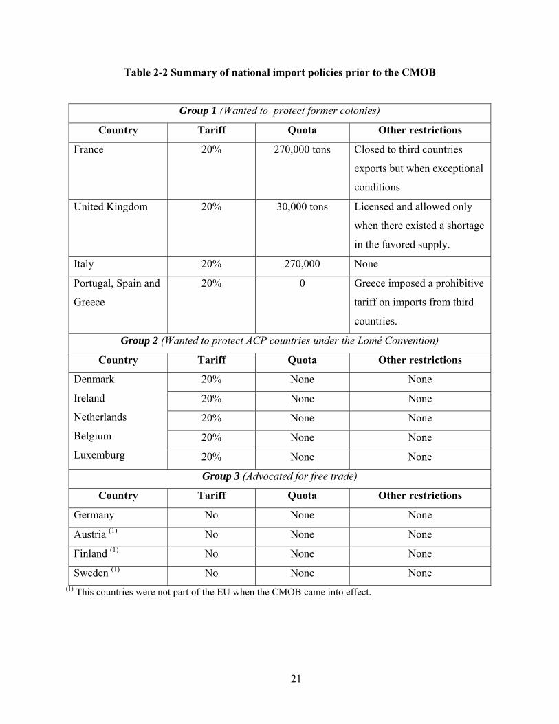
Table 2-2 Summary of national import policies prior to the CMOB

Group 1 (Wanted to protect former colonies)

Country Tariff Quota Other restrictions

France 20% 270,000 tons Closed to third countries

exports but when exceptional

conditions

United Kingdom 20% 30,000 tons Licensed and allowed only

when there existed a shortage

in the favored supply.

Italy 20% 270,000 None

Portugal, Spain and

Greece

20% 0 Greece imposed a prohibitive

tariff on imports from third

countries.

Group 2 (Wanted to protect ACP countries under the Lomé Convention)

Country Tariff Quota Other restrictions

20% None None

20% None None

20% None None

20% None None

Denmark

Ireland

Netherlands

Belgium

Luxemburg 20% None None

Group 3 (Advocated for free trade)

Country Tariff Quota Other restrictions

Germany No None None

Austria (1) No None None

Finland (1) No None None

Sweden (1) No None None (1) This countries were not part of the EU when the CMOB came into effect.

21

22

Table 2-3 Overseas territories’ production subject to price compensation

Overseas territory Maximum Production

subject to compensation

1991 production Excess (%)

Canary Islands 420,000 339,450 23.73

Guadeloupe 150,000 116,124 29.17

Martinique 219,000 181,069 20.94

Madeira 50,000 N.A N.A

Crete 15,000 N.A N.A

Total 854,000 636,643 24.00

Source: “Patiño, Maria I., M. Andrea. El régimen de acceso al mercado de la Unión Europea”.

23

Table 2-4 Duty free import quantity limits for ACP suppliers and export levels in the period 1994-2000

Actual imports (Tons) Country Duty free quota

(Tons) 1994 1995 1996 1997 1998 1999 2000

Cote d’Ivoire (2) 155,000 - - 13,684 122,045 114,664 141,924 140,916

Cameroon 155,000 148,921 113,121 109,978 170,734 191,925

Suriname(2) 38,000 27,861 33,438 22,227 24,162 17,853 28,467 28,064

Somalia (2) 60,000 - - 13,540 13,457 4,551 0 0

Jamaica (2) 105,000 75,595 82,832 66,858 67,999 55,588 41,428 30,973

Saint Lucia (2) 127,000 - - 79,877 52,602 56,861 53,579 47,692

Saint Vincent/

Grenadine

82,000 - -

Dominica (2) 71,000 - - 27,260 27,053 22,543 22,755 18,058

Belize (1) (2) 40,000 - 34,409 35,027 27,613 36,979 37,826

Cape Verde 4,800

Grenada 14,000 4,504 4,695 1,451 59 47 501 507

Madagascar 5,900 - - - -

Total 857,700 107,960 120,965 408,227 455,525 409,698 496,367 495,961

Source: CORBANA, 1993 and United Nations Statistics. (1) Remember that just part of Belize’s exports enjoys preferred treatment in the EU. (2) Exports estimated from banana imports reported by the EU.

Table 2-5 Annual average exports of main Latin American banana suppliers to the EU

(1980-1999)

Country Total

Exports

Exports to

the EU

Share of

imports to the

EU

Share into EU

total imports

Colombia 10,719.1 4,290.4 40.03 15.5

Costa Rica 13,034.4 5,730.7 43.97 20.7

Ecuador 17,567.3 3,931.9 22.38 14.2

Guatemala 4,025.6 497.1 12.35 1.8

Honduras 9,953.9 2,162.9 21.73 7.8

Nicaragua 845.0 259.0 30.65 0.9

Mexico 778.0 0.0 0.00 0.0

Panama 7,766.8 4,701.2 60.53 17.0

Dominican Republic 70.6 8.5 12.04 0.0

Total Latin America 71,951.6 27,734.4 38.55 100.0 (1) Hundred of tons. Source: United Nations. Comisión Económica para América Latina y El Caribe. Tendencias y Perspectivas de las Exportaciones de Banano de América Latina y El Caribe. 1993

24

Table 2-6 Austria, Finland and Sweden average banana imports (1990-2000)

Country 1990 1991 1992 1993 1994 1995 1996 1997 1998 1999 2000

Austria 144 154 150 146 144 111 96 94 88 102 93

Finland 70 73 86 96 169 66 58 60 58 64 62

Sweden 143 160 162 153 154 147 149 159 175 185 187

Total 357 387 398 395 466 324 303 313 321 351 341

Difference

respect to quota

-4 -34 -45 -42 -113 29 50 40 32 2 12

Hundred of tons. Source: FAO Statistics

25

Table 2-7 Human Development Index (HDI) of the EU banana suppliers

Country Region Human development

index

Rank

(1999)

GDP per capita

($US) 1

Dominica* ACP 0.873 - 3778

Grenada * ACP 0.843 - 3295

Saint Lucia * ACP 0.838 - 4505

Saint Vincent and

the Granadillas (a)

ACP 0.836 - 3018

Costa Rica LA 0.821 41 2942

Mexico LA 0.790 51 5036

Panama LA 0.784 52 3397

Belize ACP 0.776 54 3045

Colombia LA 0.765 62 2093

Suriname ACP 0.758 64 1657

Brazil LA 0.750 69 3525

Philippines Others 0.749 70 1032

Jamaica ACP 0.738 78 1487

Ecuador LA 0.726 84 1109

Cape Verde ACP 0.708 91 1400

El Salvador LA 0.701 95 2007

Nicaragua LA 0.635 106 459

Honduras LA 0.634 107 856

Guatemala LA 0.626 108 1637

Madagascar ACP 0.462 135 239

Ivory Coast ACP 0.426 144 808

Source: Human Development Reports. 1999 The HDI combines the real purchasing power per capita, life expectancy at birth, education in terms of adult literacy and school enrollment. * The index was not reported for these countries in 1999. The value shown corresponds to 1994.

26

CHAPTER 3 - Import demand for bananas in the European Union

There has been some controversy regarding whether an inverse demand system would be

more appropriate for analyzing the EU banana market than a quantity dependent demand system.

Supporters of the inverse demand base their hypothesis on the fact that banana imports in the EU

had historically been regulated by quotas on non-preferred suppliers. Therefore, quantities have

been predetermined by the quota level and prices adjusted to them. A regular demand system

assumes that quantities are determined based on the price level prevalent in the EU.

Nevertheless, two arguments can be used to justify the use of a regular demand system to

analyze the EU banana market. First, only imports from Latin America were limited by the

established quotas in the EU banana market. Consequently, only imports from this region might

be better explained by an inverse demand equation. Domestic and import demands from ACP are

properly explained based on the assumption that quantities adjust to price changes. Second, the

quota-tariff system has been substituted by a tariff-only import regime. This implies that inverse

demand equations are no longer adequate descriptions of banana demand in the EU. Since one of

the goals of this thesis is to provide policy makers with a well defined set of demand parameters

to be used on subsequent welfare and market analysis, the relevant model, the one that best

describes the most current market structure is a regular demand system.

However, following the idea that at least the demand equation for Latin America should

be inversely specified (prices adjusting to quantities), a regular and an inverse demand system

are estimated. The first corresponds to the almost ideal demand system (AIDS) and the second to

the inverse almost ideal demand system (IAIDS). The goal of estimating both models is to

determine whether the parameter estimates obtained from both of them are consistent in terms of

the way consumers in the EU consider bananas from different regions substitutes or

complementary goods.

The rest of this chapter is organized in three sections. The next one describes the

theoretical aspects of both demand systems estimated. The other details the data used on the

estimation and the last one presents and discusses the results obtained form the model estimation.

27

The Almost Ideal Demand System The Almost Ideal Demand System (AIDS) proposed by Deaton and Muellabauer in 1980

has been widely used to estimate systems of import demand equations. Two of its desirable

characteristics are that it exactly satisfies the axioms of choice and allows testing for

homogeneity and symmetry of the parameters (Deaton and Muellabauer). Those two conditions

ensure the estimation of a theoretically justifiable import demand system. The system is derived

from an indirect utility function, V(p,m), of the form shown in equation (1):

)(ln)(ln)ln(),(

pbpaMMpV −

= (1)

Where

∑ ∑∑= = =

γ+α+α=4

1

4

1

4

10 lnln5.0)ln()(ln

i i jjiiji ppppa (2)

∏= jjppb ββ0)(ln (3)

For the purpose of this study, i and j represent four different exporting regions. The first

corresponds to Latin America, the main supplier of the EU. The second is composed of the

countries from Africa, the Caribbean and Pacific that have traditionally enjoyed preferred access

to the EU market. The third region comprises the communitarian countries, which are mainly

overseas territories of Greece, Spain, France and Portugal. The last exporting region comprises

the rest of the world thus i, j = 1, …, 4 and i ≠ j. p is a price vector containing import prices from

each exporting region i; M is total expenditure in bananas in the EU, and 0α , iα , ijγ and iβ are

the parameters to be estimated.

By solving equation (1) for M, the expenditure function can be recovered as shown in

equation (4):

)()(),( papbupE U= (4)

Where b(p) and a(p) correspond to the definitions previously given and U is utility level.

By Shephard’s lemma, differentiating the log of this function with respect to the log of each

price, a set of compensated share equations ( ) is obtained. These equations represent the share

of each exporting region into total EU imports and are of the form shown in equation (5):

ciw

28

∑ ∏=

++=n

iiijiji

ci

ipUpw1

0ln βββγα (5)

After solving equation 5 for U and substituting the solution back into the compensated

share equation, uncompensated share equations are obtained:

))(ln(lnln1∑=

−++=n

iijijii paMpw βγα (6)

By estimating three of these equations simultaneously (one must be dropped to avoid

singularity of the variance-covariance matrix), a set of parameters specific for the EU banana

market are derived. To be consistent with the general demand restrictions, adding up,

homogeneity and symmetry were imposed on the system as shown in equations (7) to (9).

Adding up

(7)

0=∑n

jijγ 0,0,1

11=== ∑∑∑

==

n

iij

n

ii

n

ii γβα

Homogeneity

(8)

0=∑n

jijγ

Symmetry jiij γγ =

(9)

Price ( ijε ) and income ( imε ) elastiticies can be calculated by deriving the uncompensated

share equations with respect to the appropriate variable as depicted in equations (10) and (11)

respectively.

iji

n

ijijiiij

ij w

pδ

γαβγε −

+−=

∑=1

)ln( (10)

1−β

=εi

iiM w

(11)

Where ijδ is the Kronecker delta, taking a value of 1 when i=j and zero otherwise.

Compensated elasticities are derived from the above elasticities using the following relationship,

derived from the Slutsky identity.

iMjijcij w ε−ε=ε (12)

29

These elasticities are meaningful since they are a representation of the substitution

relationships between exporting regions, allowing us to exactly determine whether imports from

the different regions are either complements or substitutes.

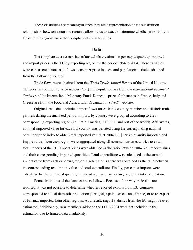
Data The complete data set consists of annual observations on per-capita quantity imported

and import prices in the EU by exporting region for the period 1964 to 2004. These variables

were constructed from trade flows, consumer price indices, and population statistics obtained

from the following sources.

Trade flows were obtained from the World Trade Annual Report of the United Nations.

Statistics on commodity price indices (CPI) and population are from the International Financial

Statistics of the International Monetary Fund. Domestic prices for bananas in France, Italy and

Greece are from the Food and Agricultural Organization (FAO) web site.

Original trade data included import flows for each EU country member and all their trade

partners during the analyzed period. Imports by country were grouped according to their

corresponding exporting region (i.e. Latin America, ACP, EU and rest of the world). Afterwards,

nominal imported value for each EU country was deflated using the corresponding national

consumer price index to obtain real imported values at 2004 US $. Next, quantity imported and

import values from each region were aggregated along all communitarian countries to obtain

total imports of the EU. Import prices were obtained as the ratio between 2004 real import values

and their corresponding imported quantities. Total expenditure was calculated as the sum of

import value from each exporting region. Each region’s share was obtained as the ratio between

the corresponding real import value and total expenditure. Finally, per capita imports were

calculated by dividing total quantity imported from each exporting region by total population.

Some limitations of the data set are as follows. Because of the way trade data are

reported, it was not possible to determine whether reported exports from EU countries

corresponded to actual domestic production (Portugal, Spain, Greece and France) or to re-exports

of bananas imported from other regions. As a result, import statistics from the EU might be over

estimated. Additionally, new members added to the EU in 2004 were not included in the

estimation due to limited data availability.

30

Descriptive statistics for the data are shown in Table 3.1. Notice that Latin America is

the main supplier of bananas to the EU. Per capita imports from this region averaged 4 kg a year

during the period 1964 – 2004. However, imports from this region were the most variable, likely

the result of the varied import regimes that have ruled the EU banana market during the analyzed

period. Average per-capita imports from ACP and the EU are very similar. Nevertheless, exports

from the ACP are more stable over time.

Bananas from Latin America are the cheapest at the border (without accounting for

tariffs) and prices from this region are less variable than import prices from other regions.

Bananas from communitarian countries are the most expensive, followed by the ACP. Import

prices from other suppliers are lower than from those two regions but still are not competitive

with respect to Latin America.

Results from the demand systems estimation Table 3.2 presents the parameter estimates obtained from the two AIDS models

estimated. The first, and the one used for further analysis, includes the four exporting regions.

The second one excludes rest of the world from the estimation. The objective of estimating this

second model was to determine how sensitive elasticitites were to the inclusion of the ROW as a

region because of its low share in the EU banana market.

In the case of the four-region model, direct estimation yielded thirteen parameters while

the other six were recovered from the theoretical restrictions imposed on the model. Eighteen out

of nineteen coefficients are significantly different from zero at the 5% confidence level and the

other at the 10%. Hence elasticitites, calculated as a function of the parameters, are likely quite

robust.

Demand elasticities obtained are shown in Table 3.3. They were calculated at each data

point and then averaged over time to obtain a single parameter value. The numbers in

parentheses are approximate t-values obtained by dividing the average elasticity by its

corresponding standard deviation.

The four own price elasticities have the expected negative sign and are significantly

different from zero at the 10% level. Import demand for bananas in the EU from all regions but

the rest of the world (ROW) is relatively inelastic. Demand for domestic product is the least

sensitive to own price changes (-0.23), followed by ACP (-0. 41) and Latin America (-0.97). On

31

the other hand, import demand from ROW is relatively elastic and therefore more sensitive to

own price changes (-1.66).

Expenditure elasticities indicate that bananas from the EU, ACP and Latin America are

normal goods. However, demand for bananas from the EU and ACP vary proportionately less

than expenditure changes. The opposite occurs to import demand from Latin America which is

relatively more sensitive to expenditure changes. The coefficients for these three regions are

significant at the 5% level. Contrary to this, income elasticity estimated for the rest of the world

is negative and not significantly different from zero. This result will be discussed in more detail

when the three-region model’s results are presented.

Compensated price elasticities are also shown and used to determine whether bananas

from the four different sources are complements or substitutes. The advantage of this procedure

is that the income (expenditure) effect is eliminated, letting us analyze the pure price effect and

categorize the goods as q-net complements or q-net substitutes. As expected, bananas from Latin

American and the other regions are substitutes. Nevertheless only parameters for ACP and ROW

are significant. Domestic and ACP bananas are also substitutes as expected but cross price

elasticities for these two regions are not significantly different from zero. Results obtained for

the ROW indicate that imports from this region are considered complementary to bananas

supplied by ACP and the EU. Even though this result is only significant for the case of the ACP,

it is worthwhile to expand on the reasons that may explain this result.

While the objective is to estimate a demand system at the consumer level, the data used is

at the wholesale level. It would be expected then that a fraction of total imports are for industrial

or processing uses, which might deviate from the consumer demand relations found in the data.

Additionally, the inclusion of ROW as a fourth region in the demand system might affect the

results because of the low share it has in the EU banana market.

This share has also decreased over time. For example, imports from this region accounted

for 12% of the total imported value in 1964 by the EU but only 0.33% in 2004. On average,

imports from this region accounted for just 2% of total banana imports in the EU during the

analyzed period. This and the questionable elasticity values obtained for this region justified the

estimation of another demand model excluding this region.

Parameter estimates are presented in Table 3.2. A total of thirteen parameters were

obtained in this case, eight of them directly from the model estimation and five more were

32

recovered from the theoretical restriction imposed on the model before its estimation. All

parameters are significant.

Conclusions drawn from own-price and expenditure elasticities are similar to those

obtained from the four-region model. Demand for bananas from Latin America is the most price

sensitive, followed by ACP and demand for communitarian bananas. Expenditure elasticities

have the same signs and are very close in value. Indeed they are the same for Latin America and

the EU. Compensated elasticities are not as robust as those obtained in the previous model.

However, some conclusions are comparable to it. For example, bananas from Latin America and

all other regions are substitutes and demands from the EU and ACP are complements. In this

case the result is significant while in the previous model it was not.

Because there are no evident gains in excluding ROW from the demand estimation, all

subsequent analysis are based on the four-region model. Nevertheless it is important to keep in

mind some of the limitations of the results, notably negative expenditure elasticity for ROW and

some questionable complementary relations in the demand for bananas from different regions.

33

Table 3-1 Descriptive statistics of trade data used in demand estimation

Variable Mean St. Deviation Minimum Maximum

Quantities (kg per capita)

Latin America 4.07 2.59 0.87 8.46

EU 1.38 0.57 0.62 2.83

ACP 1.55 0.34 0.95 2.16

Others 0.16 0.22 0.01 0.71

Prices (real 2004 $/ton)

Latin America 217.17 194.51 16.073 847.28

EU 279.14 222.53 18.012 802.89

ACP 261.81 213.72 12.314 776.33

Others 227.03 221.56 7.4721 862.38

Expenditure (real $ per capita) 2.24 2.51 0.06 9.66

The data set contains 42 observations.

34

Table 3-2 Parameters estimated from the AIDS model

AIDS (4 regions) AIDS (3 regions) Parameter Coefficient Parameter Coefficient

α0 96.66** α0 155.210*

(96.57) (2.673) α1 17.44** α1 27.280*

(19.408) (3.517) α2 -3.32** α2 -4.527*

(-3.8925) (-2.405) α3 -10.21** α3 -21.753*

(-13.485) (6.618) α4 -2.91** n/a n/a (-4.321) β1 0.17** β1 0.167*

(18.539) (9.940) β2 -0.03** β2 -0.029*

(-4.1714) (-2.854) β3 -0.1** β3 -0.137*

(-13.693) (-11.067) β4 -0.04** n/a n/a (-6.025) γ11 2.76** γ11 4.428*

(9.023) (-4.223) γ12 -0.57** γ12 -0.885*

(-3.622) (-2.847) γ13 -1.75** γ13 -3.543*

(-9.2364) (-4.090) γ14 -0.44** n/a n/a

(-3.2157) γ22 0.13** γ22 0.325*

(1.8371) (-2.847) γ23 0.34** γ23 0.560*

(4.2922) (2.438) Table continues…

35

Table continued… AIDS (4 regions) AIDS (3 regions)

Parameter Coefficient Parameter Coefficientγ24 0.1** n/a n/a

(-2.9189) γ33 1.14** γ33 2.982*

(-7.244) (3.900) γ34 0.27** n/a n/a

(-3.5116) γ44 0.07* n/a n/a

(-1.618) * Indicates significant values at the 5% level

36

Table 3-3 Elasticities from the 4-region AIDS model

Uncompensated elasticities Price/Quantity

Latin America EU ACP ROW

Latin America -0.97** -0.40** 0.09 11.18

(-6.31) (-4.28) (0.50) (1.06)

EU -0.32** -0.23* -0.10** -1.21

(-5.57) (-1.53) (-2.19) (-1.04)

ACP -0.15* -0.18** -0.41** -4.00

(-1.63) (-3.40) (-2.00) (-1.01)

Rest of the World 0.08** -0.05** -0.10** -1.66**

(2.68) (-4.09) (-3.142) (-2.51)

Expenditure elasticity 1.36** 0.86** 0.52** -0.21

(18.06) (30.52) (4.04) (-0.88)

Compensated elasticities Price/Quantity

Latin America EU ACP ROW

Latin America -0.31* 0.02 0.33** 8.98

(-1.48) (0.25) (2.03) (1.08)

EU 0.01 -0.02 0.03 -2.26

(0.29) (-0.20) (0.392) (-0.94)

ACP 0.19* 0.03 -0.27* -5.04

(1.41) (0.41) (-1.69) (-0.96)

Rest of the World 0.11* -0.03 -0.09** -1.67**

(1.43) (-1.02) (-2.34) (-2.45)

* Indicates significant at the 10% level ** Indicates significant at the 5% level

37

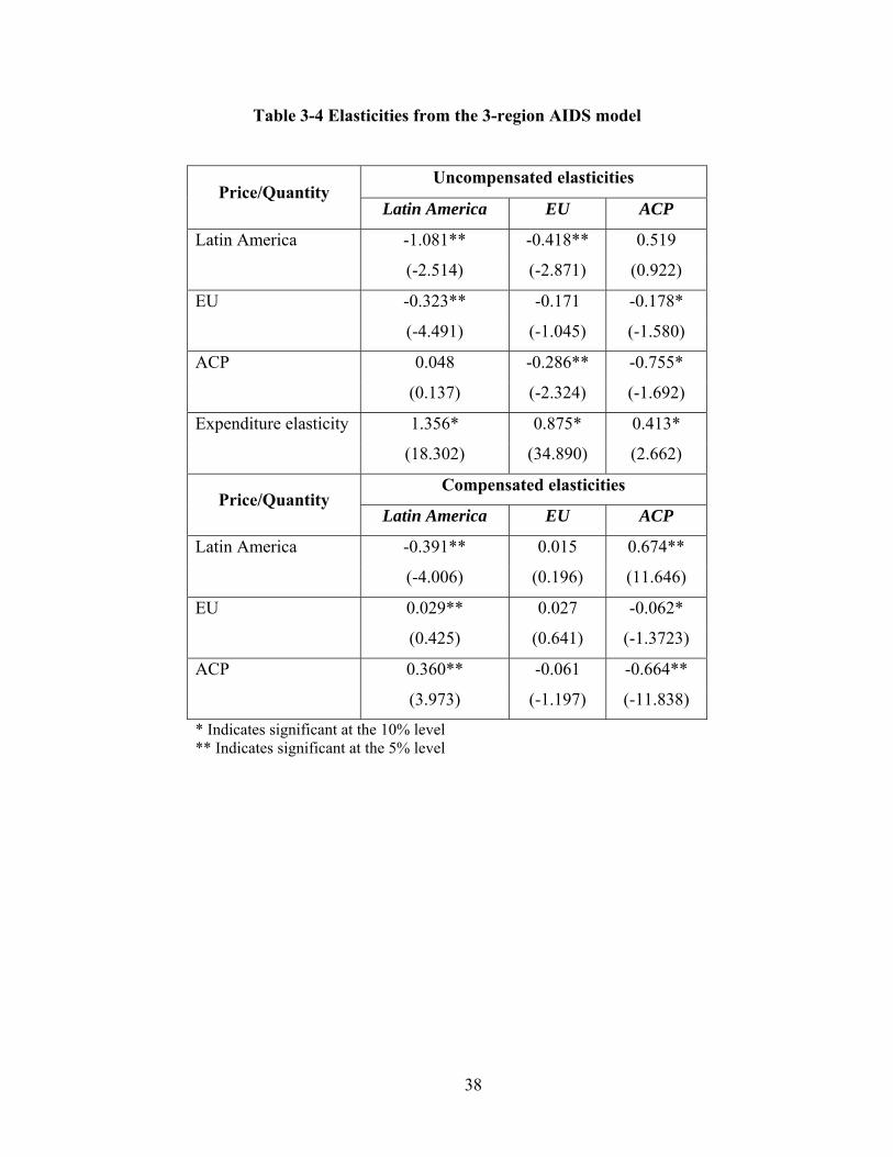
Table 3-4 Elasticities from the 3-region AIDS model

Uncompensated elasticities Price/Quantity

Latin America EU ACP

Latin America -1.081** -0.418** 0.519

(-2.514) (-2.871) (0.922)

EU -0.323** -0.171 -0.178*

(-4.491) (-1.045) (-1.580)

ACP 0.048 -0.286** -0.755*

(0.137) (-2.324) (-1.692)

Expenditure elasticity 1.356* 0.875* 0.413*

(18.302) (34.890) (2.662)

Compensated elasticities Price/Quantity

Latin America EU ACP

Latin America -0.391** 0.015 0.674**

(-4.006) (0.196) (11.646)

EU 0.029** 0.027 -0.062*

(0.425) (0.641) (-1.3723)

ACP 0.360** -0.061 -0.664**

(3.973) (-1.197) (-11.838)

* Indicates significant at the 10% level ** Indicates significant at the 5% level

38

CHAPTER 4 - Economic effects of the new import policy

Modeling of the import policy As explained in Chapter 2, prior to January 2006 the EU banana market was regulated by

a tariff-quota system designed to protect EU communitarian and ACP producers. Under this

scheme, imports from ACP countries enjoyed duty free access up to 750,000 tons. Above this

quota, imports were taxed at a 380 Euros/ton rate (approximately US $373). Additionally,

imports from non-preferred suppliers were subject to a tariff of 75 Euros/ton (approximately US

$93) within a 2,750,000 ton quota. Out-of-quota imports paid a tariff of 680 Euros/ton

(approximately 2004 US $845). This quota was increased by 100,000 tons in 2002, as part of the

second stage of an agreement signed between the EU and the US.

To summarize Chapter 2, recall that the EU defined a new import system to replace the

existing tariff-quota scheme. The new regime came into effect in January of 2006 and required

the removal of all quotas but also a higher tariff level for non-preferred suppliers. The duty-free

quota for ACP was increased to 775,000 tons in an attempt to continue to safeguard this region’s

access to the EU market. However, ACP’s exports above this quota level must abide by the same

regulations imposed on non-preferred suppliers.

The effect of the transition from one import regime to another on the major banana

suppliers of the EU is what is evaluated in the following two chapters. To model this transition it

was necessary to convert the Latin American quota level to what I refer to as an “equivalent

tariff” to avoid several complications related to the use of a non-continuous supply function as

implied by a tariff-quota situation. The tariff-quota supply equation would be as shown in

equation (13).

[ ]iip

iii quotapsMins ),,( τ= (13)

This specification indicates that export supply of region i (si) is given by the minimum

quantity between the quota imposed on the specific region (quotai) and a quantity that depends

on a export price (pip) and region-specific tariff level ( ). iτ

The obvious drawback of working with this supply specification is that it is not a

continuous function, making it cumbersome to convert it to its total differential form.

39

Additionally, the modeling issue in the simulations would have required estimation of the

elasticity of supply with respect to the quota; information that is not only unavailable, but

questionable as to its meaning as well. Estimating an equivalent tariff allow one to subsume the

quota component in the supply equation. Supply can then be solely expressed as a function of

import prices and tariff levels.

Using as a base case a pre-2006 producer surplus measure, one can calculate the tariff

level that would have made Latin American producers as well off as the quota. This equivalent

tariff was calculated as the difference between the actual price received by producers and a

hypothetical price under which they would be willing to supply a quantity equal to the quota

level, subject to achieving the same producer surplus as under the quota restriction.

Figure 4.1 represents the pre-2006 market equilibrium for Latin America. Here, Q0 and Pc

are the equilibrium quantity and price respectively. D is the demand curve faced by this region

and the line PaAS represents the supply curve that would prevail under the import quota

situation. Pa is the minimum price producers are willing to export to the EU market and A marks

the minimum price at which producers are willing to export Q0 based upon the upward-sloping

portion of the supply curve.

Figure 4-1 Pre-2006 equilibrium in the Latin American banana market

40

Under this scenario, producer surplus is given by the shaded area under the equilibrium

price (Pc) and above the supply curve. Geometrically for ease of estimation, this area can be

divided in two parts, one given by the rectangle formed by points PbAEPc and the other by the

triangle PaAPb. Producer surplus can then be estimated as the sum of those two areas as shown

in equations (14) and (15).

( ) ( ) 00 **5.0* QPPQPPPS abbc −+−= (14)

or (15) ( 0*5.05.0 QPPPPS abc −−= )

Figure 4-2 Pre-2006 LAT simulated equilibrium under the absence of import quotas

The calculated producer surplus was then used to simulate an equivalent new market

equilibrium under a non-quota scenario, as the one depicted in Figure 4.2. The shaded area

represents producer surplus and is equal to the producer surplus previously estimated under the

quota scenario. What is needed is the hypothetical price (Pd) that would make producers as well

off as under the quota while supplying quantity Q0. This price can be obtained from the producer

surplus equation for the non-quota scenario (PS).

0*)(*5.0 QPaPdPS −= (16)

41

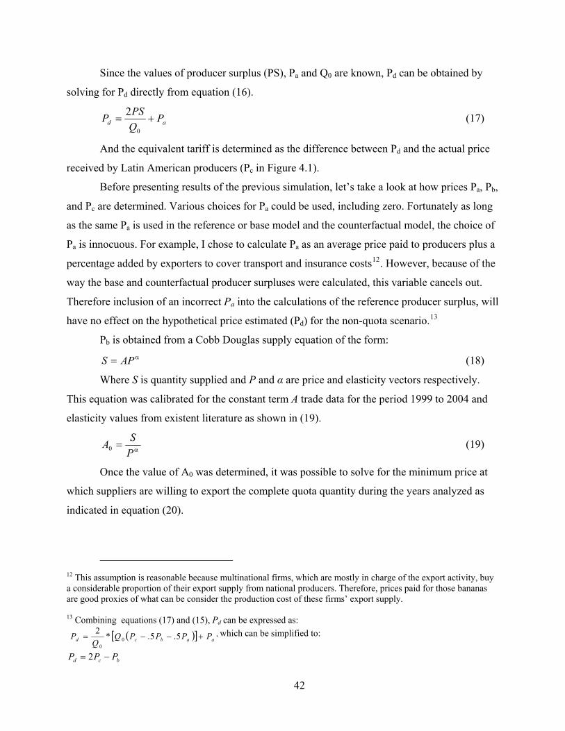
Since the values of producer surplus (PS), Pa and Q0 are known, Pd can be obtained by

solving for Pd directly from equation (16).

ad PQPSP +=

0

2 (17)

And the equivalent tariff is determined as the difference between Pd and the actual price

received by Latin American producers (Pc in Figure 4.1).

Before presenting results of the previous simulation, let’s take a look at how prices Pa, Pb,

and Pc are determined. Various choices for Pa could be used, including zero. Fortunately as long

as the same Pa is used in the reference or base model and the counterfactual model, the choice of

Pa is innocuous. For example, I chose to calculate Pa as an average price paid to producers plus a

percentage added by exporters to cover transport and insurance costs12. However, because of the

way the base and counterfactual producer surpluses were calculated, this variable cancels out.

Therefore inclusion of an incorrect Pa into the calculations of the reference producer surplus, will

have no effect on the hypothetical price estimated (Pd) for the non-quota scenario.13

Pb is obtained from a Cobb Douglas supply equation of the form: α= APS (18)

Where S is quantity supplied and P and α are price and elasticity vectors respectively.

This equation was calibrated for the constant term A trade data for the period 1999 to 2004 and

elasticity values from existent literature as shown in (19).

α=PSA0 (19)

Once the value of A0 was determined, it was possible to solve for the minimum price at

which suppliers are willing to export the complete quota quantity during the years analyzed as

indicated in equation (20).

12 This assumption is reasonable because multinational firms, which are mostly in charge of the export activity, buy a considerable proportion of their export supply from national producers. Therefore, prices paid for those bananas are good proxies of what can be consider the production cost of these firms’ export supply. 13 Combining equations (17) and (15), Pd can be expressed as: ([ aabcd PPPPQ

QP +−−= 5.5.*2

00

)] , which can be simplified to:

bcd PPP −= 2

42

α

⎟⎟⎠

⎞⎜⎜⎝

⎛=

1

0

0

AQ

Pb (20)

Where A0 is the calibrated constant term from equation (23) and Q0 is the quota level

applied to Latin American countries in the period 1999 to 2004. Results of this calculation are

presented in Table 4.1 for two alternative short-run elasticity values (0.75 and 1.5) based on the

values reported by FAO (2005).

Table 4.2 presents the equivalent per unit tariff for the previous two elasticity scenarios.

Notice that as expected the more elastic the supply is, the less “penalized” Latin American

producers are from the quota imposed on their exports to the EU banana market. These values

were used for calibrating the equilibrium displacement model presented in the next section.

Equilibrium displacement model To simulate the effects of the new EU import regime of bananas on the major producer

regions, an equilibrium displacement model (EDM) was used. The EU banana market was

decomposed, following the same criteria used for demand estimation, into four regions or

markets defined by Latin America; the African, Caribbean, Pacific countries (ACP); the EU

(representing local production) and rest of the world (ROW).

The use of this model, instead of a partial equilibrium framework, takes into account not

only the direct effects of the new import regime in the entire EU market but also the indirect

effects from the interrelations among the different exporting regions. As shown by the cross

price elasticities obtained from the AIDS model, the four exporting regions are related on the

demand side.

In this way, if the import price from a certain region changes as a result of the new import

regime, not only that region’s quantities demanded and supplied will react, but also demand and

supply from other regions. Ultimately, all import prices will react to those quantity variations,

which will have an impact on the equilibrium prices and quantities of the other markets. This

chain of events will continue until a new equilibrium has been simultaneously reached in all

markets. The model that follows presents these interactions.

The general model is initially described by the following set of equations:

),,( iii zMdd cp= Demand for bananas from region i (21)

43

),( ip

iii pss τ= Supply of bananas from region i (22)

ii sd = Market clearing condition for quantities (23)

ip

ici pp τ=− Market clearing condition for prices (24)

Where i refers to each exporting region (i.e. Latin America, ACP, EU and others); M is

total annual expenditure in bananas in the EU; represents a vector of n demand shifters for

region i’s demand; is a vector of consumer prices; is producer price in region i; and,

represents per-unit import tax for region i. Prices and quantities are endogenous in the model

while shift variables, expenditure, and import tariffs were exogenously determined outside the

model.

iz

cp pip

iτ

The system is then converted to its log differential form following the steps described

below. First, total differential of equations (21) to (24) were taken, which transformed the

previous set of equations to a system of the form:

in

N

n i

iicj

jcj

ii z

zd

MMd

ppd

d Δ∂∂

+Δ∂∂

+Δ∂∂

=Δ ∑∑== 1

4

1

(25)

ii

ipj

jpj

ii

sp

ps

s τΔτ∂∂

+Δ∂∂

=Δ ∑=

4

1

(26)

ii sd Δ=Δ (27)

ip

ici pp τΔ=Δ−Δ (28)

where indicates absolute change (i.e. ) with upper indexes 1 and 0

referring to after the shock and initial values of the variable respectively. Next, equations (25) to

(28) were rearranged to express them in terms of elasticities and log differentials. Starting with

expression (25), both sides of the equation were multiplied by 1/ to yield:

Δ 01iii ddd −=Δ

id

i

inN

n i

i

i

i

i

cj

jcj

i

i

i

dz

zd

dM

Md

dp

pd

dd Δ

∂∂

+Δ

∂∂

+Δ

∂∂

=Δ ∑∑

== 1

4

1

;

Then, the terms on the right hand side (RHS) were multiplied by j

j

pp

, MM and

i

i

zz

respectively to derive the following equation:

44

in

in

in

inN

n in

i

i

icj

cj

i

cj

jcj

i

i

i

zz

dz

zd

MM

dM

Md

pp

dp

pd

dd Δ

∂∂

+Δ

∂∂

+Δ

∂∂

=Δ ∑∑

== 1

4

1

;

Finally, terms were combined together to express this equation in terms of elasticities and

proportional changes as shown by (25’).

∑∑==

++=N

nininii

i

cjiji zMpd

1

~~4

1

~~ζμε (25’)

Where ijε represents elasticity of demand i with respect to price j; iμ is expenditure

elasticity of demand i; inζ is the elasticity of demand i with respect to variable zin; and

symbolizes the proportional change of variable x (i.e.

~

ix

0

01

i

ii

xxx −

).

A similar procedure was used to transform the three other equations of the system. For

example, the supply equation was first multiplied by 1/ and then each resulting term of the

RHS was multiplied by

is

pj

pj

pp

and i

i

ττ

respectively, to obtain the following expression:

i

i

i

i

i

ipj

pj

i

pj

jpj

i

i

i

ss

pp

sp

ps

ss

ττΔτ

τ∂∂

+Δ

∂∂

=Δ ∑

=

4

1

;

Which after grouping and re-ordering of terms can be expressed as: ~~4

1

~

iipj

jiji ps τυ+η= ∑

=

(26’)

Where ijη is the elasticity of supply i with respect to price j and iυ is the elasticity of

supply i with respect to its tariff.

The following expression was derived from equation (23) after taking the total

differential and multiplying each side by 1/ : iq

i

i

i

i

qd

qs Δ=

Δ

Making use of the fact that quantity demanded and supplied must change in the same

proportion for the market to be in equilibrium, the following identity must hold: iii sdq == this

equation (23) is equivalent to:

45

~~

ii ds = (27’)

To convert the price clearing condition (24) into relative change form, each term of the

original equation was multiplied by i

ici

ci

pp

ττ

, and di

di

pp

respectively to obtain:

pi

pip

ii

iic

i

cic

i pp

ppp

p Δ=ττ

τΔ−Δ

pi

piii

ci

ci pppp

~~~

=ττ−⇒

Then, by multiplying both sides by pip

1 and re-arranging terms, equation (24) becomes:

~~~p

ipi

iip

i

cic

i ppp

pp =

ττ−

~~~

)1( piiii

ci pp =−+⇒ πτπ (28’)

Where iπ indicates the percentage tariff on imports from region i and is calculated as the

ratio between per-unit tariff and producer price14.

To summarize, the equilibrium displacement model of the EU banana market is described

by the following set of equations:

∑∑==

++=N

ninini

ijiji zMpd

1

~~4

1

~~ζμε (25’)

~~4

1

~

iipj

jiji ps τυ+η= ∑

=

(26’)

~~

ii sd = (27’)

~~~

)1( piiii

ci pp =−+ πτπ (28’)

The system was reduced by substituting equation (28’) into (26’) as follows: ~~~4

1

~)1( iiiii

ci

jiji ps τυ+⎥

⎦

⎤⎢⎣

⎡πτ−π+η= ∑

=

(34’’)

14 From (20), . So, pii

ci pp +τ= 1+

τ= c

i

ici

ci

ppp

46

By doing so, the model was solely expressed in terms of endogenous changes in

quantities (supplied and demanded) and consumer prices ( ). Grouping these endogenous

variables in the RHS and assuming that changes in all exogenous variables but the tariff level are

zero

cjp

15, the following system of three equations was obtained:

04

1

~~=−∑

=j

cjiji pd ε (29)

iij

ijici

jiiji ps

~~

4

1

~4

1

~)1( τ

⎟⎟⎟

⎠

⎞

⎜⎜⎜

⎝

⎛πη−υ=π+η− ∑∑

==

(30)

0~~=− ii ds (31)

Equations (29) to (31) can be expressed in matrix form as M X = Y. Where M contains

all relevant price elasticities, X embodies price and quantity changes and Y comprises

information on exogenous variable changes. These matrices are defined as:

⎥⎥⎥

⎦

⎤

⎢⎢⎢

⎣

⎡

−−−

=0IIηI0ε0I

'M , ⎥⎦⎤

⎢⎣⎡=

~

i

~

i

~

i psdX and, ⎥⎥⎥

⎦

⎤

⎢⎢⎢

⎣

⎡

=B

~'

B

0τν

0Y

Where:

I 4 x 4 identity matrix

0 4 x 4 null matrix

ε 4 x 4 matrix of demand elasticities with elements εij

-η' 4 x 4 matrix with elements )1( iij π+η

η 4 x 4 matrix of supply elasticities with elements ηij

ν' 4 x 1 vector with elements ∑=

π−4

1jiiji ην

~v 1 x 4 vector of tariff level changes

0B 4 x 1 null vector

15 Under this assumption, terms and ∑ become zero. ~

iMμ=

ζN

ninin z

1

~

47

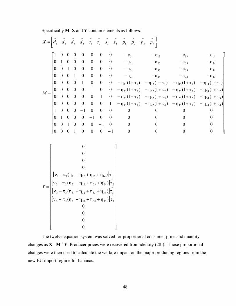
Specifically M, X and Y contain elements as follows.

⎥⎦⎤

⎢⎣⎡=

~

4

~

3

~

2

~

1

~

4

~

3

~

2

~

1

~

4

~

3

~

2

~

1 ppppssssddddX

⎥⎥⎥⎥⎥⎥⎥⎥⎥⎥⎥⎥⎥⎥⎥⎥⎥

⎦

⎤

⎢⎢⎢⎢⎢⎢⎢⎢⎢⎢⎢⎢⎢⎢⎢⎢⎢

⎣

⎡

−−

−−

τ+η−τ+η−τ+η−τ+η−τ+η−τ+η−τ+η−τ+η−τ+η−τ+η−τ+η−τ+η−τ+η−τ+η−τ+η−τ+η−

ε−ε−ε−ε−ε−ε−ε−ε−ε−ε−ε−ε−ε−ε−ε−ε−

=

000010001000000001000100000000100010000000010001

)1()1()1()1(10000000)1()1()1()1(01000000)1()1()1()1(00100000)1()1()1()1(00010000

00001000000001000000001000000001

444443442441

334333332331

224223222221

114113112111

44434241

34333231

24232221

14131211

M

[ ][ ][ ][ ]

⎥⎥⎥⎥⎥⎥⎥⎥⎥⎥⎥⎥⎥⎥⎥⎥⎥⎥

⎦

⎤

⎢⎢⎢⎢⎢⎢⎢⎢⎢⎢⎢⎢⎢⎢⎢⎢⎢⎢

⎣

⎡

τη+η+η+ηπ−ν

τη+η+η+ηπ−ν

τη+η+η+ηπ−ν

τη+η+η+ηπ−ν

=

0000

)(

)(

)(

)(0000

~

44443424144

~

33433323133

~

22423222122

~

11413121111

Y

The twelve equation system was solved for proportional consumer price and quantity

changes as X =M-1 Y. Producer prices were recovered from identity (28’). Those proportional

changes were then used to calculate the welfare impact on the major producing regions from the

new EU import regime for bananas.

48

Calibration of the equilibrium displacement model As shown by equations (29) to (31), supply and demand elasticities as well as policy

variables were needed to calibrate the equilibrium displacement model. Demand parameters were

obtained from the estimation of the Almost Ideal Demand System. Supply elasticities were taken

from existent literature and corresponded to the same values used to calculate the equivalent

tariff for Latin America.

To model policy changes from one import regime to the other, it was assumed that only

the quota imposed on Latin American imports was binding. This assumption is justified based on

the quota realities (see Chapter 2). Since this quota was converted to its equivalent tariff, only

data on tariff levels and tariff changes for all regions were required. The elasticity of supply with

respect to the tariff level (υ) was approximated by the own price supply elasticity as an increase

in the tariff level would have the same impact as a decrease in the prices paid to exporters.

Finally, the percentage tariff (π) was calculated as the ratio between total tariff revenue received

by the EU from each region and total value exported by the respective region.

Results of the equilibrium displacement model Table 4.3 shows the results of the equilibrium displacement model for two different

scenarios corresponding to the same elasticity values used in the equivalent tariff calculation. It

is important to mention that the results discussed in this section are based on Monte Carlo

simulations as will be explained in more detail in the following chapter. Briefly, the use of

Monte Carlo analysis allows bounds to be placed on the calculated point estimates of price and

quantity changes in each market in order to make probabilistic inferences about the possible

changes in the EU banana market as a means of providing a sensitive analysis.

Results indicate that under the new import regime, prices are likely to increase in all

markets. In the first scenario, where Latin American supply is relatively inelastic (η = 0.75),

there is an 88% chance that the import price for this region will increase. Price is also likely to

rise in the rest of the world, ACP and the EU. However, the probability of communitarian

producers obtaining a higher price is lower than for ROW and ACP suppliers whose probability

of a price increase is around 61% and 63% respectively versus a 54% chance for EU producers.

49

50

Quantity exported by each region on the other hand is likely to be less affected by the

import regime change. Again, Latin American exports have the greatest possibility of increasing

(77% probability). The probability of imports from the EU growing is 54% and contrary to what

happened to price increases, the chances of the ACP and ROW of augmenting their sales to the

EU market are low respect to the EU. ACP producers face the lowest odds of increasing their

export level with just a 7% chance whereas there is 31% probability that shipments from ROW

increase in the short run.

Finally, from the results it was also possible to determine the chances each region has of

increasing their share in the EU banana market. As expected by the previous results, Latin

American producers are the ones with the greatest opportunity for increasing their market share

(74% probability), followed by the EU (24%), the ACP and ROW (with 15% and 14%

respectively).

Information on the new average price and quantities are also included in Table 4.3. These

values are the average new price and quantity in each market and can be compared to their initial

levels under the previous quota-tariff import regime.

Notice that results are very stable across the two Latin American-supply scenarios. The

chance of a price increase in both cases is the same while the probabilities of quantity increases

are just slightly higher for the EU, ACP and ROW and lower for Latin America under the second

scenario. The same happens to the possibility of each region increasing its market share.

However, results still support the idea that Latin American producers are the most likely to

increase their presence in the EU banana market.

Table 4-1 Results of supply equation calibration

LAT Export Supply Elasticity = 0.75 LAT Export Supply Elasticity = 1.50 Period Import Price Quota level

Estimated constant (A0)1 Pb2 Estimated constant (A0) Pb

1999 416.43 2,750,000 34225.39 346.72 371.27 379.98

2000 361.61 2,750,000 38636.37 294.97 465.92 326.60

2001 391.72 2,750,000 36202.08 321.71 411.15 354.99

2002 436.38 2,750,000 35250.82 333.34 369.21 381.39

2003 627.36 2,850,000 27121.63 495.87 216.36 557.76

2004 820.96 2,850,000 22895.93 621.51 149.28 714.31

Average3 509.08 2,783,333 32205.00 406.32 326.74 457.29

(1) A0 corresponds to the constant term of the export supply curve of Latin America. (2) Pb represents the minimum price Latin American producers are willing to supply the quota level. (3) Aerage value was used to calculate the equivalent tariff under the two export supply elasticity scenarios.

51

Table 4-2 Latin American banana supply: equivalent tariff calculation

LAT Export Supply Elasticity = 0.75

Period Import price (pc)1 Pb2 Pa

3 Producer surplus 4 Implicit price (pd)5 Equivalent tariff

1999 416.43 346.72 310.61 241,352,300 486.14 69.71

2000 361.61 294.97 302.89 172,376,276 428.25 66.64

2001 391.72 321.71 292.73 232,356,968 461.72 70.01

2002 436.38 333.34 302.27 326,074,811 539.41 103.04

2003 627.36 495.87 296.45 658,914,924 758.84 131.48

2004 820.96 621.51 317.58 1,001,540,150 1,020.42 199.45

Average equivalent tariff 106.72

LAT Export Supply Elasticity = 1.50

Period Import price (pc) Pb Pa Producer surplus Implicit price (pd) Equivalent tariff

1999 416.43 379.98 310.61 195,621,089 452.88 36.45

2000 361.61 326.60 302.89 128,892,291 396.63 35.02

2001 391.72 354.99 292.73 186,595,251 428.44 36.72

2002 436.38 381.39 302.27 259,998,783 491.36 54.98

2003 627.36 557.76 296.45 570,734,215 696.96 69.60

2004 820.96 714.31 317.58 869,301,901 927.62 106.65

Average equivalent tariff 56.57

(1) Actual import price in constant 2004 US $. (2) Minimum price Latin American producers are willing to supply the quota level (from Table 4.1). (3) Vertical intercept of Latin America export supply curve. (4) In constant 2004 US $. (5) Simulated price that would make producers as well of as the quota.

52

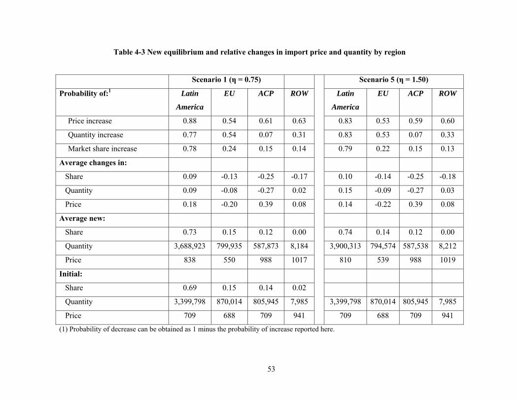
53

Table 4-3 New equilibrium and relative changes in import price and quantity by region

Scenario 1 (η = 0.75) Scenario 5 (η = 1.50)

Probability of:1 Latin

America

EU ACP ROW Latin

America

EU ACP ROW

Price increase 0.88 0.54 0.61 0.63 0.83 0.53 0.59 0.60

Quantity increase 0.77 0.54 0.07 0.31 0.83 0.53 0.07 0.33

Market share increase 0.78 0.24 0.15 0.14 0.79 0.22 0.15 0.13

Average changes in:

Share 0.09 -0.13 -0.25 -0.17 0.10 -0.14 -0.25 -0.18

Quantity 0.09 -0.08 -0.27 0.02 0.15 -0.09 -0.27 0.03

Price 0.18 -0.20 0.39 0.08 0.14 -0.22 0.39 0.08

Average new:

Share 0.73 0.15 0.12 0.00 0.74 0.14 0.12 0.00

Quantity 3,688,923 799,935 587,873 8,184 3,900,313 794,574 587,538 8,212

Price 838 550 988 1017 810 539 988 1019

Initial:

Share 0.69 0.15 0.14 0.02

Quantity 3,399,798 870,014 805,945 7,985 3,399,798 870,014 805,945 7,985

Price 709 688 709 941

709 688 709 941

(1) Probability of decrease can be obtained as 1 minus the probability of increase reported here.

54

CHAPTER 5 - Welfare analysis of the import-only regime

As has been previously stressed, the goal of this study is to determine the effect of the

new import regime on banana producers. Although consumer welfare is also important, banana

producers are more vulnerable to market changes. Whereas expenditure on bananas does not

represent a significant share of a consumer’s total expenditure, for producers, a small decrease in

their market share might imply important losses and may even force them out of the market.

Therefore, this section focuses on the estimation of the economic impact of the new import

policy on banana producers from all regions but mainly those on Latin America and the ACP.

Welfare changes are measured as the change in producer surplus as detailed in the following

section.

Producer surplus Because each region’s market equilibrium not only depends on own price but also on the

price of bananas from the competing regions, a price change in one region would affect demand

and supply in each market. The EU market and that of its suppliers is depicted in Figure 5.1 Even

though prior to 2006, the Latin American market behaved differently than the other three regions

due to the existence of a binding quota, the calculation of the equivalent tariff explained in the

previous section, enabled to analyze all four markets under the same scheme.

In the diagram, S0 and D0 represent the initial supply and demand curves respectively

(here, we have used linear curves for simple explanation). Initial market equilibrium is given by

price level p0 and quantity q0. Due to the enforcement of a new import policy, supply and

demand changes can be expected in all regions. Demand changes will be determined mostly by

the substitution or complementary relationship between the bananas from different origins. For

example, as demand for ACP and Latin America are substitutes, an increase in the price of Latin

American bananas will increase the demand for ACP produce. Changes in the supply will be

determined by how sensitive the supply from each region is to its own price changes.

Figure 5-1 Equilibrium of major supplier regions in the EU banana market

55

The new equilibrium will be given at a new point such as f, with p1 and q1 being the new

price and quantity levels. Whether these variables are higher or lower than their initial values can

not be determined a priori. The place of the new equilibrium depends on the combined effect of

the supply and demand curve movements, which ultimately depends on the cross-price demand

and own-price supply elasticities in each region.

For expositional purposes a hypothetical scenario is depicted where initial producer

surplus is given by the triangle p0bI0 and then changes to p1fI1 due to the new import regime. The

difference between those two areas is a measure of the change in producer surplus ( ), which

can be expressed as:

iPSΔ

1100 fIpbIpPSi −=Δ (32)

Defining g as the shift in the supply equation and assuming that supply and demand shifts

are parallel, the triangle ghI1 is equivalent to p0bI0. So, changes in producer surplus for each

region can be expressed as:

111 fIpghIPSi −=Δ (33)

This difference is equal to the area ghfp1, which can be decomposed into two smaller

areas: the rectangle gmfp1 and the triangle mfh. Those areas can be calculated respectively as:

111 )qp-(gdmfp = (34-a)

)q-)(qp-0.5(gmfh 011= (34-b)

Therefore, the change in producer surplus for each region i ( iPSΔ ) is given by:

))(qp-(d5.0)qp-(g 0i

1i

1ii

1i

1ii qPSi −+=Δ (35)

Where gi is the shift of region i’s supply, and are initial and new equilibrium prices

in region i respectively and and are initial and new equilibrium quantities.

0ip 1

ip0iq 1

iq

In share form (35) can be expressed as:

ii1ii qw5.0qw ΔΔ+Δ=Δ iPS (36)

Where and represent changes in region i’s share and in quantity supplied,

respectively.

iwΔ iqΔ

56

Multiplying the first and second terms of the RHS of equation (44) by i

i

ww

and

i

i

i

i

ss

ww

respectively, the change in producer surplus can be expressed in terms of relative changes

as shown by (37).

iii

i

i

iii

i

ii sw

ss

ww

swww

PSΔΔ

+Δ

=Δ 21

[ ]iiiii swsPS ~1~w 21+=Δ⇒ (37)

Total change in producer surplus for the EU market is given by the sum of the changes in

producer surplus in each region:

∑=

Δ=Δ4

1iiEU PSPS (38)

Precision Measures of the Welfare Estimates As discussed earlier, the equilibrium displacement model that solves for the parameters

necessary to calculate welfare effects of the new import regime was parameterized based, on

among other variables, demand elasticities of the EU market. These elasticities were calculated

as non-linear functions of parameters estimated from the Almost Ideal Demand System (AIDS).

Therefore, for each different set of parameters there exist a new set of elasticities that differ from

the others depending on the magnitude of the difference among the parameter sets and the way

those parameters are related within each set. Likewise, there is a solution for the EDM model and

new welfare estimations for each parameter set. Making use of these relationships, Monte Carlo

simulations based on the demand parameters obtained from the AIDS model were used to derive

measures of precision for the producer surplus estimates.

To do this, I started with the fact that each parameter obtained from the AIDS model is

characterized by its point estimate and its standard deviation. Additionally, the complete

parameter set is also described by a variance-covariance matrix that depicts the degree of

correlation between each parameter. Ignoring this correlation between coefficients would not

generate samples with exactly the same characteristic as the original multiple-variable population

(Fan et al. 2002).

57

Assuming normality of all parameters, imposing the population correlation pattern on a

sample data set was done by decomposing the covariance matrix using the procedure proposed

by Fan et .al (2002). First, to define the structure of the relationship between the demand

parameters in a way that could be imposed on the sample data, the variance-covariance matrix

generated when solving the AIDS model was decomposed using the principal component factor

extraction method. In general, this procedure generates new variables, also known as factors that

are linear combinations of the variables analyzed.

In this case, decomposition of the AIDS parameter variance-covariance matrix generated

a new pattern matrix of dimension 13 X 13 because the procedure was performed on the 13

coefficients directly generated by the demand model. The information generated here was used

to simulate coefficient values of the other six parameters that were not directly estimated by the

AIDS model but that were recovered from the economic restrictions imposed before the demand

system instead. The SAS code for this step is provided in Appendix B.

In a second step, k random variables were generated and then multiplied by the factor

pattern matrix to impose the population correlation and generate a sample of correlated variables

of size k. Finally, using data on parameters means and standard deviations in a Monte Carlo

framework, a distribution of demand parameters was generated, which enabled me to build

distributions of elasticities and hence, distributions of the solutions to the EDM and, thus, of

producer surplus.

To ensure the analysis is based on reliable coefficients, once the parameter distribution

was obtained, elasticities were calculated at each data point and then tested to ensure that each

elasticity set conformed to economic theory. In other words, each elasticity set was tested for

negativity (negative own price elasticities) and curvature16 (negative semi-definite Hessian of

compensated elasticities). If any given parameter set did not conform to any of these two

restrictions, the data point was eliminated. The goal is to obtain what is termed “truncated

distribution” of elasticities in order to perform the requisite simulations. Even with the faster

computer, the simulations are nonetheless very time consuming. When the process was

terminated, I had obtained a truncated distribution with 267 observations that was compliant with

all theoretical economic restrictions. Descriptive statistics of this parameter distribution and

estimated market shares are shown in Table 5.1.

16 Adding up, homogeneity and symmetry were imposed when calculating the AIDS model.

58

Notice that on average the parameter values of the truncated distribution are almost the

same as the point estimates of the original data set obtained from the AIDS model. However, the

truncated distribution presents lower variability, measured as the standard deviation of the

parameters. This was a result of imposing restrictions on the parameters, which eliminated

extreme data points that did not conform to economic theory. Average market shares simulated

at each data point for the four regions are also very close to their real values in 2003, the base

year used in the calculations.

Results Table 5.2 shows producer surplus changes that result from the EU switching to a new

import regime under two alternative supply elasticity values. It also includes information on

price, quantity and share changes (solution of the EDM) as well as the new equilibrium levels of

those variables for each producing region.

The difference between the two scenarios is the value of Latin American supply

elasticity, which in the first case is less elastic simulating a shorter time horizon (η = 0.75). The

second scenario models a more elastic supply for Latin America and can be viewed as a larger

time horizon where producers had more flexibility in responding to market changes by adjusting

their production levels and changing their marketing practices. For both scenarios, own price

supply elasticities for the other regions are 0.4 in the case of the European Union, 0.5 for ACP’s

and 0.8 for the rest of the world (ROW). These values are based on the estimates by Arias

(2006).

From the first scenario, based on the average changes in producer surplus, it can be

concluded that Latin American and EU producers gain from the new import regime, while ACP

suppliers are harmed and exporters from the rest of the world are not affected. However,

additional information generated from the parameter distribution, instead of just point estimates,

indicates that these results are not certain.

For example, even though mean changes in producer surplus for Latin America and the

EU are positive, the probability of producers from Latin America gaining from the new regime is

79%. This means that there is a 21% chance that producers from this region might be harmed by

59

the tariff-only import regime. This is also evident when considering the 90% confidence interval

of the producer surplus for Latin America, which ranges between -$368,247 and $816,005. 17

What is perhaps more interesting is that such high variability might be an indication that

the tariff-only import regime is statistically no different from the import policy enforced by the

Common Market Organization for bananas (CMOB). If this were the case, one could conclude

that EU has been successful in adopting an alternative import system that is consistent with

WTO regulations and at the same time maintains Latin American access to its market, at least in

the short run.

A similar analysis can be done for the EU. Simulation results indicate that producers

from this region gained an average of $57,868 as result of the new import regime. However, the

chance of producers being positively affected is only 28%. In other words, there is a probability

of 78% that suppliers from this region lose due to the import regime change. Changes in

producer surplus for this region vary between -$34,595 and $400,326, thus, again, one might

conclude that the new regime leads to no change, at least not a statistically significant one.

Additionally, even though it seems that producers from the ACP region are the net losers

from an import system change, statistics of the estimated producer surplus changes indicate that

this measure is not significantly different from zero. That is, on average producers from this

region are not really harmed by the new import system. The same result was obtained for the rest

of the world, where point estimates indicate that producers from this region gained $1 from the

import system switch. It can be concluded therefore that the tariff-only and the CMOB import

regimes are equivalent from the perspective of these two regions.

When analyzing price and quantity changes, all regions face the possibility of obtaining a

higher price for their product, with Latin America having the better odds of increasing their

equilibrium price, followed by the rest of the world, ACP and the EU in that order. Results are

not as promising for quantity increases. For example, the probability for Latin American and EU

producers of increasing their quantity supplied is 77% and 54% respectively. Meanwhile, the rest

of the world faces a probability of 31% of increasing their quantity exported to the EU while this

possibility is just 7% for the ACP region.

These results comply with the ones obtained from analyzing producer surplus changes.

Latin America has the greatest possibility of increasing its market share in the EU banana market

17 Surplus is measured in constant 2004 US $.

60

(78%), followed by the EU (24%), ACP (15%) and the ROW (14%). 18 However, there is not

certainty that any region will gain or lose from the new import regime.

For the second scenario, average gains are higher for Latin America, the EU and the

ROW and average losses are lower for the ACP. If we maintain the assumption that this scenario

models a larger time horizon (in the form of a more elastic supply for the EU), results fit the idea

that producers are less affected because they had more time to adjust to the new market

conditions in the EU banana market.

Even though Latin America still gains on average, producer surplus changes are lower

under this scenario. Additionally, changes in the producer surplus for the other regions are not

significantly different from zero. Probabilities of gaining from the switch to a tariff-only import

system are about the same for Latin America and the EU but a little bit more promising for ACP

and ROW suppliers.

Tables 5.3 to 5.5 show different scenarios maintaining the same supply elasticities used

for scenarios 1 and 2, but varying the tariff level imposed by the EU. Three alternative tariff

levels were analyzed. The first corresponds to the initial tariff proposed by the EU of 230

Euros/ton and that was ruled out by a WTO panel. The second is the lower tariff suggested by

the EU after the WTO resolution (176 Euros/ton) and the third corresponds to the tariff level

requested by the Latin American region at the beginning of the consultation process with the

WTO (75 Euros/ton).

Contrary to what one might think, a higher tariff does not harm Latin American

producers as much as it does ACP suppliers. This is most evident from scenario 3, in which a

higher tariff level (230 Euros/ton) implies a higher average producer surplus for Latin America

and higher average losses for the ACP region compared to the base scenario. This indicates that

the duty free quota conceded to producers from this region is in fact binding and that their ability

of overcoming the effects of an import tariff is limited. This result is not surprising as this has

been the argument used by ACP producers and EU policy makers to protect this region against

competition from lower cost Latin American producers.

18 The higher possibility of the ACP gaining market share with respect to the ROW derives from the higher average change in price that the first region might face.

61

The better gains for Latin America derive from a greater quantity increase. Under the 230

Euros/ton tariff scenario the new average quantity would have been around 200 thousand tons

higher than under the base scenario. ACP exported quantity is on the other hand lower.

As happened in the previous cases however, there is no certainty that Latin America

would have benefited from the adoption by the EU of such a tariff level and again, even though

changes in producer surplus for ACP are negative on average, there is no statistical evidence that

those changes are different from zero. That is, one cannot conclude that ACP producers would

have been made worse off if the EU had set its tariff level at this level.

Results from scenario 4 are qualitatively equal to the previous one. The difference is in

the magnitude of the welfare effects, especially for Latin America and the ACP. Here, a lower

tariff translates into lower average losses for the ACP and lower average gains for Latin

America. Results suggest correlation between the magnitudes of gains for Latin America and

losses for the ACP region. This idea is sustained by results from the last scenario, which

analyzed the effects of imposing a tariff of just 75 Euros/ton. Under such market conditions,

ACP average welfare reduction and Latin American gains would have been the lowest of all

possible scenarios.

Interestingly, conclusions drawn from simulations under alternative tariff levels are

opposite to the ideas expressed by most exporters and EU policy makers when trying to negotiate

the tariff level. That is, it has been shown here that the lower the tariff the less benefited Latin

America producers would have been because it would have enabled ACP producers to compete

under more favorable conditions against Latin American exports.

Final remarks Even though it is still early for exporters to determine whether they will be harmed or

helped by the import regime, as it has only been in effect for less than a year, some Latin

American countries such as Costa Rica and Panama have admitted that their exports have not

decreased as a result of the new import policy. This position is in contrast with that maintained

62

by other exporting countries, especially Ecuador, who argues that the 176 Euros/ton tariff level is

prohibitive.19

As discussed, results from the simulation analysis show that a null hypothesis of no

change for producers from the new import policy cannot be rejected. However, this does not

mean that the tariff-only import system will affect all countries in the same way. This is

especially true when considering the differences in production costs prevalent among producer

countries within a region. As Chacon (2004) showed in an analysis of the effect of the first stage

of the US-EU agreement in the main Latin American producers, even though the quota level for

these countries increased, only Costa Rican and Colombian producers benefited from it. Ecuador

and the rest of the producers from this region were made worse off by the new import policy

scheme.

This situation might be repeated again and results from the analysis are consistent with

such a prognosis. For example, it is not certain that Latin America will gain from the new import

regime. The possible losses reported by the simulation exercises might correspond to losses

faced by countries such as Ecuador. Additionally, the fact that the simulations suggest the

possibility that the old and new import regimes are equivalent, is in line with Costa Rica and

Panama confessing that during the present year their exports to the EU have not importantly

changed as a result of the import regime changing.

Finally, results are in line with some conclusions reached by other authors. Guyomard

(2004) for example indicated that ACP producers are the most vulnerable to the new import

regime and that they will be negatively affected unless they are compensated and their banana

production becomes more competitive. This situation is likewise reflected in our results.

Anania (2006) concluded that the 176 Euros/ton tariff is not high enough to maintain

Latin American access to the EU banana market. She showed that the new import regime

benefits non-preferred suppliers. Our results show that on average and in probabilistic terms this

a plausible outcome of the EU switching regimes.

19 Ecuador proposed for Latin American producers to call another WTO panel to ask for a reduction of the 176 Euros/ton tariff to their bananas. Costa Rica did not support this position as they support a gradual decrease of the quota to avoid an overflow of the market. (La Nación. August 15 and October 20, 2006)

63

64

Table 5-1 Comparison of simulated distribution and descriptive statistics of the demand

parameter set

Simulated distribution N=267 Point Estimates from AIDS

Parameter Mean St. Deviation Parameter Mean St. Deviation

α1 17.44 0.66 α1 17.42 0.90

γ12 -0.57 0.18 γ12 -0.58 0.16

γ13 -1.75 0.18 γ13 -1.73 0.19

γ14 -0.44 0.14 γ14 -0.43 0.13

β1 0.17 0.01 β1 0.17 0.01

α0 96.66 0.99 α0 96.58 1.00

α2 -3.32 0.57 α2 -3.28 0.84

α3 -10.21 0.42 α3 -10.18 0.75

γ23 0.34 0.08 γ23 0.34 0.08

γ24 0.10 0.03 γ24 0.10 0.03

γ34 0.27 0.07 γ34 0.27 0.08

β2 -0.03 0.01 β2 -0.03 0.01

β3 -0.10 0.00 β3 -0.10 0.01

Simulated market shares 2003 market shares

Region Average St. Deviation Region Average St. Deviation

Latin America 0.66 0.12 Latin America 0.69 n/a

EU 0.15 0.08 EU 0.15 n/a

ACP 0.15 0.09 ACP 0.14 n/a

ROW 0.03 0.02

ROW 0.02 n/a

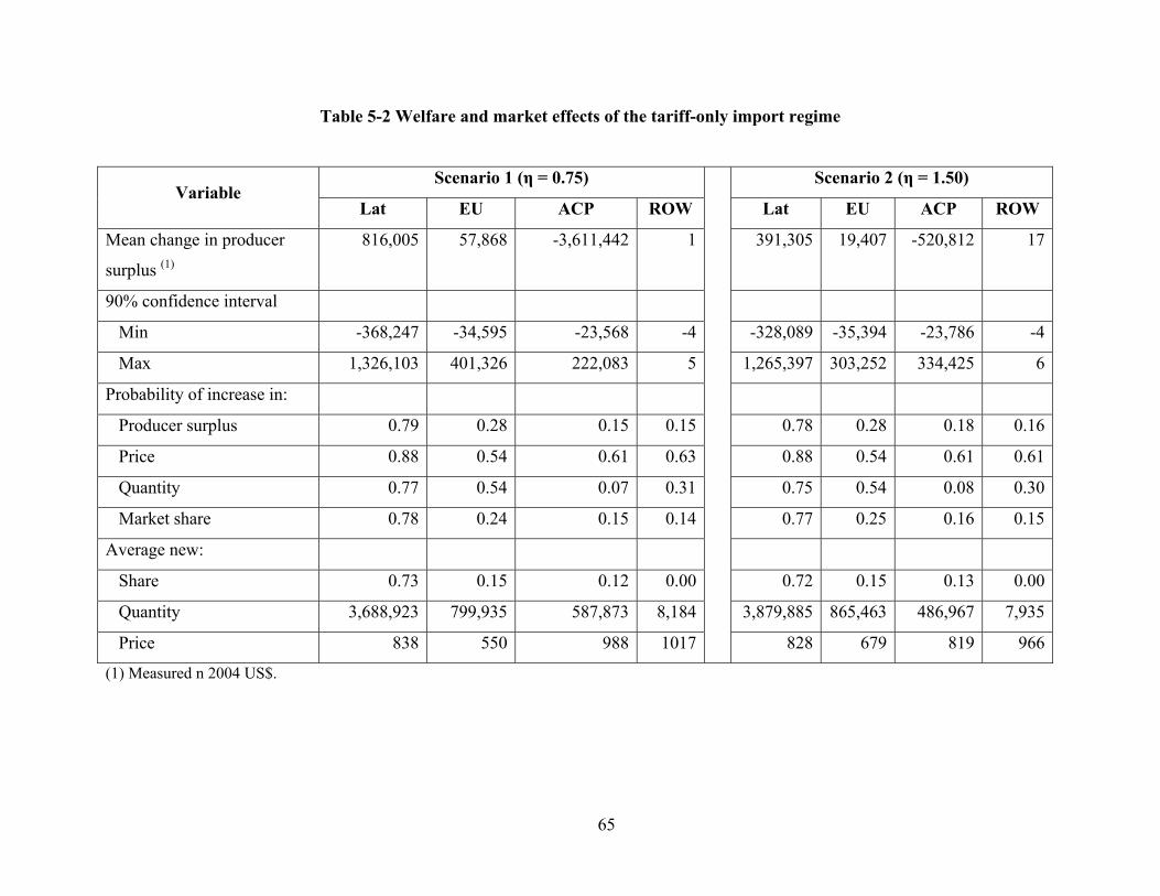
Table 5-2 Welfare and market effects of the tariff-only import regime

Scenario 1 (η = 0.75) Scenario 2 (η = 1.50) Variable

Lat EU ACP ROW Lat EU ACP ROW

Mean change in producer

surplus (1)

816,005 57,868 -3,611,442 1 391,305 19,407 -520,812 17

90% confidence interval

Min -368,247 -34,595 -23,568 -4 -328,089 -35,394 -23,786 -4

Max 1,326,103 401,326 222,083 5 1,265,397 303,252 334,425 6

Probability of increase in:

Producer surplus 0.79 0.28 0.15 0.15 0.78 0.28 0.18 0.16

Price 0.88 0.54 0.61 0.63 0.88 0.54 0.61 0.61

Quantity 0.77 0.54 0.07 0.31 0.75 0.54 0.08 0.30

Market share 0.78 0.24 0.15 0.14 0.77 0.25 0.16 0.15

Average new:

Share 0.73 0.15 0.12 0.00 0.72 0.15 0.13 0.00

Quantity 3,688,923 799,935 587,873 8,184 3,879,885 865,463 486,967 7,935

Price 838 550 988 1017

828 679 819 966

(1) Measured n 2004 US$.

65

66

Table 5-3 Welfare and market effects of three alternative tariff levels in the EU banana market

Scenario 3 (τ = 230 Euros/ton) Scenario 4 (τ = 187 Euros/ton) Scenario 5 (τ = 75 Euros/ton) Variable

Lat EU ACP ROW Lat EU ACP ROW Lat EU ACP ROW

Mean change in producer

surplus

823,844 57,236 -3,679,865 1 731,943* 64,678 -3,015,875 2 391,305* 19,407 -520,812 17

90% confidence interval

Min -358,406 -34,634 -23,581 -4 -303,605 -34,531 -23,535 -4 -328,089 -35,394 -23,786 -4

Max 1,318,597 396,765 225,856 5 1,252,070 379,093 193,657 5 1,265,397 303,252 334,425 6

Probability of increase in:

Producer surplus 0.79 0.28 0.15 0.15 0.79 0.31 0.15 0.17 0.78 0.28 0.18 0.16

Price 0.87 0.54 0.61 0.63 0.91 0.55 0.62 0.66 0.88 0.54 0.61 0.61

Quantity 0.79 0.54 0.07 0.32 0.54 0.55 0.07 0.28 0.75 0.54 0.08 0.30

Market share 0.78 0.24 0.15 0.14 0.78 0.27 0.15 0.16 0.77 0.25 0.16 0.15

Average new:

Share 0.73 0.14 0.12 0.00 0.72 0.15 0.12 0.00 0.72 0.15 0.13 0.00

Quantity 3,731,984 798,843 587,805 8,190 3,293,545 809,961 588,500 8,132 3,879,885 865,463 486,967 7,935

Price 832 547 988 1,018 889 569 990 1,014 828 679 819 966

CHAPTER 6 - Summary and conclusions

The EU is one of the world’s biggest importers of bananas and, as such import policies

enforced by this trade union are likely to have a great impact on the major producers of bananas.

Aiming to protect communitarian producers and exporters from selected ex-colonies of Africa,

the Caribbean and Pacific and to honor previous agreements, the EU unified its import policy for

bananas in 1993. This policy, known as the Common Market Organization for Bananas,

generated one of the most controversial trade disputes in history. After several modifications of

the original regime, in January 2006, the EU changed its import regime to satisfy a World Trade

Organization mandate and to honor an agreement signed with the United States in 2000.

The controversy generated during and after the enforcement of both import regimes has

inspired authors to analyze this market extensively. However, there are still many gaps to fill in

the literature that are addressed in this study, especially the lack of adequate estimation of

demand parameters and of statistical simulation analysis to test for the significance of the results

obtained from the analysis.

The objectives of this project were to provide a detailed overview of the history of the

trade dispute, to estimate a theoretically consistent demand system to generate reliable

parameters and then to use these parameters in a system-wide welfare analysis of the EU banana

market. The latter focused on the impact of the new import policy in the major producing areas

as these are the agents that are most likely to be affected by the new import regime.

Additionally, Monte Carlo analysis was used to derive sensitivity measures of the welfare and

market change estimates.

Analysis of results indicates that on average Latin American and EU communitarian

producers benefit from the new regime while ACP exporters will be harmed. However, the

sensitivity analysis, which allowed making probabilistic inferences about the statistical

significance of these point estimates, indicates that those results are not certain. The hypothesis

that the new import regime will not affect the major suppliers of the EU banana market was not

rejected. This might indicate that the policy enforced by the Common Market Organization for

Bananas and the current tariff-only import regime are statistically equivalent. In other words, the

EU expertly forced a tariff level that will leave much as status quo.

67

Another interesting result is that the duty –free quota allowed to ACP producers is not

enough to safeguard the market interests of this region. A higher tariff level, such as that initially

proposed by the EU, will no better protect ACP exporters from Latin American competition.

Indeed, higher import taxes benefit the through market share losses of the ACP region in the EU

banana market.

Based on opinions recently expressed by some Latin American countries regarding their

support of the new import regime and on conclusions drawn from the simulation analysis, it

seems likely that not all countries will be affected in the same way by the change in import

regimes. It would be important for future analysis to determine country-specific effects of the

new import regime. This can be achieved by estimating a demand system disaggregated by

country to generate country-specific demand elasticitites. This would enable solving a modified

equilibrium displacement model where markets are defined as individual countries and not as

regions as was done here. Finally, results of the equilibrium displacement model indicate that EU

consumers are likely to lose from the new regime due to higher prices and lower quantities. So,

future research should also address this issue.

68

CHAPTER 7 - References

Alston, J.M., Norton G.W., Pardey P.G. Science Under Scarcity: Principles and Practice for Agricultural Research Evaluation and Priority Setting. Ithaca, NY: Cornell University Press.

Anania G. “The 2005 episodes of the “banana war” serial. An empirical assessment of the

introduction by the European Union of a tariff-only import regime for bananas” University of Calabria. Working paper 06-02. www.bananalink.org.uk/index.php?option=com_content&task=view&id=168&Itemid=120

Allen, C., M. Gasiorek and A. Smith. (1998). ‘The competition Effects of the Single Market in

Europe’. European Single Market. Economic Policy. October 1998.

Arias, P. D. Hallam, L. Hubbard, L. Pascal. “The elusive tariff equivalent for the EU banana market.” FAO. Commodity Market Review 2005-2006. http://www.fao.org/docrep/008/a0334e/a0334e0g.htm

Borrell, B. “Policy Making in the EU: the bananarama story, the WTO and policy transparency” The Australian Journal of Agricultural Economics 41:2 (1997): 263-276.

Borrell, B. and K. Hanslow. “Banana Supply Elasticity.” Briefing Notes. Centre for International Economics. December 2004.

Borrell, B. and Y. Maw-Cheng. “EC Bananarama 1992: The Squeal.” The Developing Economies XXX-3 (1992): 259-283.

Borrel, B. “EU Bananarama III”. The World Bank International Economics Department International Trade Division and Latin American and the Caribbean Regional Office. Policy Research Working Paper 1386 (1994).

Cambrón, A.C. Borrador de la Carta Bananera Internacional. Banana Link. April 1998. http://members.tripod.com/alianzacoord/apm/banasust.rtf

Cascavel. Para un Régimen Bananero Sostenible. Banana Link. April 1998. http://members.tripod.com/alianzacoord/apm/cartabana.rtf

Chacón-Cascante, A. and J.M. Crespi.. “An Overview of the European Union Banana Import Policy” Revista de Agronomía Costarricense (forthcoming).

69

Chacón-Cascante, A. “Estimation of the Welfare Effects of the Banana Import Agreement between the EU and the US” Master thesis. Kansas State University. 2004.

Commission of the European Communities, “Communication from the Commission to the

Council on the ‘First Come, First Served’ Method for the banana regime and the implications of a ‘tariff only’ system. Bruselas, October, 2000.

Commodities and Trade Division, FAO. “Partial equilibrium model of the world banana market.” Working document.

Corporación Bananera Nacional (CORBANA). “Repercusiones para Costa Rica de la Aplicación de Cuotas en el Mercado Bananero de la C.E.” 1993.

De Arce, R., G. Escribano, R. Mahía. “Estimation of a tariff only level to replace the current European protection system for the banana market.” Asociación grupo de estudios Europeos y Mediterráneos (AGREEM). July 2004.

Deaton, A., Muellbauer, J. “An Almost Ideal Demand System”. The American Economic Review. 70 (1980): 312-326.

Eales, J. and L. Unnevehr. “The inverse almost ideal demand system” European Economics Review. 38 (1994): 1001-115.

Food and Agriculture Organization of the United Nations. FAOSTAT. http://faostat.fao.org/site/352/DesktopDefault.aspx?PageID=352 August 28, 2006.

Guyomard, H., Ch. Le Mouël. “The New Banana Import Regime in the European Union: A Quantitaive Assesemnt” Insitut National de la recherche Agronomique. Working paper 02-04. www.rennes.inra.fr/economie/pdf/WP02-04.pdf

Human Development Report 1999. http://hdr.undp.org/

IICA. Centro para la Integración y el Desarrollo Agroempresarial. Perfil de la actividad y del Comercio Bananero 1994. Serie de Publicaciones Miseláneas. San José, Costa Rica. Abril, 1995.

International Monetary Fund. International Financial Statistics Yearbook. Various issues.

Kersten, Lutz. “Impacts of the EU banana market regulation on international competition, trade and welfare.” European Review of Agricultural Economics 22 (1995): 321- 335.

70

71

Kox, Henk L.M. “Welfare gains from liberalized banana trade and the new international banana agreement”. Faculteit der Economische Wetenschapper en Econometrics. Serie Research Memoranda #1998-12. April 1998.

La Nación. “País lucha por baja gradual del arancel bananero en la UE.” August 15, 2006. San

José, Costa Rica. La Nación. “Costa Rica descarta apoyar a Ecuador en panel ante OMC por banano.” October 20,

2006. San José, Costa Rica. http://www.nacion.com/ln_ee/2006/octubre/20/ultima-sr867862.html

Patiño, María I., M. Andrea. El régimen de acceso al mercado de la Unión Europea. Revista

Augura. 20, no.1 (2000): 4-111. Piggott, N. “Measures of Precision for Estiamted Welfare Effects for Producers from Generic

Advertising.” Agribussiness: An International Journal. 19 (3) (Summer 2003): 379 – 391.

Tangermann, Stefan. Banana Policy: a European Perspective. The Australian Journal of Agricultural and Resource Economics. 41, no. 2 (1997): 277-282.

United Nations. World Trade Annual Report of the United Nations. Various issues.

World Trade Organization. “Hong Kong WTO Ministerial 2005: Briefing Notes Bananas Discussions continue on a long-standing issue” http://www.wto.org/english/thewto_e/minist_e/min05_e/brief_e/brief22_e.htm

World Trade Organization. Trade Policy Review: First Press Release, Secretariat and

Government Summaries. European Union: November 1997.

Appendix A - Variable definition and description

Table A-7-1 Observed variables in Chapter 3 (EU import demand for bananas)

Variable Name Description Unit / base year Source

i, j Producing regions Latin America (Lat)

European Union (EU)

Africa, the Caribbean and the Pacific (ACP)

Rest of the world (ROW)

N/A N/A

p Price vector Annual price vector containing annual import

prices from each exporting region i

2004 US $ per ton Computed as the ratio

between real import

value and quantity

imported from each

region i.

M Expenditure Annual total expenditure in bananas in the EU 2004 US $ Computed as the sum of

import value from each

region

Table continues…

72

Table continued…

Variable Name Description Unit / base year Source

iw Uncompensated share

equation

Share equation for each region i estimated based on

observed shares, total expenditure M, price vector

p and estimated coefficients.

Percentage Observed shared

computed as the ratio

between region’s i

imported value and total

expenditure M.

ijε Uncompensated own

price and cross price

elasticities

Measure of the sensibility of demand of bananas

from region i to price changes of bananas from

region j

Percentage Computed from the

AIDS model parameter

estimates

imε Expenditure elasticity Measure of the sensibility of demand of bananas

from region i to changes in total expenditure M

Percentage Computed from the

AIDS model parameter

estimates cijε Compensated own

price and cross price

elasticities

Measure of the sensibility of demand of bananas

from region i to price changes of bananas from

region j isolated of the income effect.

Percentage Computed from

observed shares,

uncompensated price

and income elasticities

q Quantity vector Vector containing imported quantity from each

region i.

Tons / year World Trade Annual

Report of the United

Nations.

ijf Flexibility Measure of the sensibility of region i’s import price

from to imported quantity changes from region j.

Percentage Computed from the

IAIDS model parameter

estimates.

73

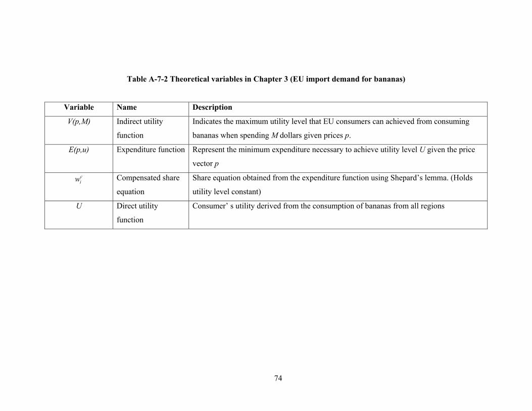
Table A-7-2 Theoretical variables in Chapter 3 (EU import demand for bananas)

Variable Name Description

V(p,M) Indirect utility

function

Indicates the maximum utility level that EU consumers can achieved from consuming

bananas when spending M dollars given prices p.

E(p,u) Expenditure function Represent the minimum expenditure necessary to achieve utility level U given the price

vector p ciw Compensated share

equation

Share equation obtained from the expenditure function using Shepard’s lemma. (Holds

utility level constant)

U Direct utility

function

Consumer’ s utility derived from the consumption of bananas from all regions

74

Table A-7-3 Variables used in Chapter 4 (Equilibrium Displacement Model)

Variable Name Description Unit / base year Source

di EU demand for

bananas from each

region i

Accounts for the quantity imported by the EU

from each region i.

Tons / year World Trade

Annual Report of

the United Nations.

iτ Per unit tariff for

region i

Import tax paid by each region i to enter the

EU market.

Euros / ton

2004 US $ / ton

Various

pp Vector of producer or

exporter prices

Prices of bananas from region i at the exporter

level.

2004 US $ per ton Computed as the

ratio between real

import value and

quantity imported

from each region i. cp Vector of consumer

prices

Prices of bananas from region i at the

consumer level.

2004 US $ per ton Computed as

producer price plus

per unit tariff . iτ

iz Vector of n demand

shifters for demand

from region i

Takes into account variables other then prices

and expenditure that have an affect on EU the

import demand of bananas.

AIDS model no shifters

Annual

N/A

Table continues…

75

Table continued…

Variable Name Description Unit / base year Source

ixΔ Total differential of a

given variable xi

Indicates absolute changes in the equilibrium

value of the variables that define the EU

banana market model (i.e. quantities, prices

and policy variables).

01iii xxx −=Δ

~

ix Proportional change in

variable xi

Change in variable xi expressed in relative

terms.

Percentage 0

01

i

ii

xxx −

ijε Elasticity of demand i

with respect to changes

in price j

Measure of the sensibility of demand of

bananas from region i to price changes of

bananas from region j

Percentage From the AIDS and

GAIDS models.

iμ Expenditure elasticity

of demand for region i

Measure of the sensibility of demand of

bananas from region i to changes in total

expenditure M

Percentage From the AIDS

model.

inζ

Elasticity of demand i

with respect to a

change in variable zin.

Measure of the sensibility of demand of

bananas from region i to changes in shifter

variable zin.

Percentage From the GAIDS

model.

Table continues…

76

Table continued…

Variable Name Description Unit / base year Source

ijη Elasticity of supply i

with respect to price j

Measure of the sensibility of region i’s export

supply to changes in region j;s export price.

Percentage B. Borrell and

Hanslow K.

iυ Elasticity of supply i

with respect to its tariff

Measure of the sensibility of region i’s export

supply to changes in its own import quota . iτ

Percentage

iπ Percentage tariff on

imports from i

Region i’s per unit import tariff expressed as a

percentage of consumer price.

Percentage Calculated as the

ratio between

consumer and

producer prices pi

ci

pp

M Parameter matrix Includes elasticity and policy variables the

parameterize the EDM.

Various Various

X Endogenous variables Relative changes in price and quantity for each

producing region under the new import

regime.

Percentage Obtained after

solving the EDM

model.

Y Market shifters Policy variables that changed with adoption of

the new import system

Various Change in tariff and

equivalent tariff

from one import

system to the other.

77

Table A-7-4 Variables used in Chapter 5 (Welfare Analysis)

Variable Name Description Unit / base year Source,

computation

iPSΔ Change in producer

surplus

How much producer surplus for region i

changes as result of the new import regime.

2004 US $ Calculated from

Equation X

(Chapter 5)

q0 Initial equilibrium

quantity in region i

Initial equilibrium quantity imported by the

EU from region i under the old import regime

Tons World Trade

Annual Report of

the United Nations.

q1 New equilibrium

quantity in region i

New equilibrium quantity imported by the EU

from region i under the new import regime

Tons Calculated from the

EDM model.

p0 Initial equilibrium

price in region i

Initial equilibrium import price from region i

under the old import regime.

2004 US $ / ton World Trade

Annual Report of

the United Nations.

p1 New equilibrium

price in region i

New equilibrium import price from region i

under the new import regime

2004 US $ / ton Calculated from the

EDM model.

78

Appendix B - Factor pattern SAS code to impose population correlation on Monte Carlo

simulated parameters

data A (type=corr);_type_='corr'; input A1 G12 G13 G14 B1 A0 A2 A3 G23 G24 G34 B2 B3; cards;

1 . . . . . . . . . . . . -6.66E-02 1 . . . . . . . . . . . -0.1264 -1.76E-03 1 . . . . . . . . . . -7.72E-02 -6.62E-04 1.02E-02 1 . . . . . . . . . 7.92E-03 -6.59E-04 -1.27E-03 -7.73E-04 1 . . . . . . . . -4.45E-03 5.33E-03 1.66E-02 7.88E-03 -1.68E-03 1 . . . . . . . -0.22786 0.12898 -3.55E-02 -2.11E-02 -2.22E-03 -3.53E-03 1 . . . . . . -0.26809 -4.65E-02 0.1252 1.07E-02 -2.62E-03 -7.04E-03 -0.3191 1 . . . . . 3.23E-02 -1.13E-02 -1.23E-03 1.72E-03 3.21E-04 -3.00E-03 -5.94E-02 1.17E-02 1 . . . . 1.82E-02 -3.67E-03 -8.53E-05 -2.67E-03 1.81E-04 -1.52E-03 -1.67E-02 1.01E-02 1.22E-03 1 . . . 3.97E-02 3.35E-03 -7.89E-03 -9.49E-03 3.98E-04 -4.51E-03 2.79E-02 -2.00E-02 -1.95E-03 8.11E-04 1 . . -2.24E-03 1.27E-03 -3.44E-04 -2.05E-04 -2.24E-05 3.04E-04 6.96E-03 -3.14E-03 -5.85E-04 -1.64E-04 2.72E-04 1 . -2.64E-03 -4.53E-04 1.25E-03 1.12E-04 -2.74E-05 9.37E-04 -3.14E-03 5.60E-03 1.13E-04 9.78E-05 -2.01E-04 -3.06E-05 1 ; proc factor n=13 outstat=facout;/*Stores the factor pattern data into the file facout*/ DATA PATTERN; SET FACOUT; IF _TYPE_='PATTERN'; DROP _TYPE__NAME_; RUN;

79