1

The effects of EU aid on receiving and sending countries A modelling approach Dawn Holland and Dirk Willem te Velde

1

12 November 2012 This report was prepared by the Overseas Development Institute and the National Institute of Economic and Social Research for ONE.

1 Dawn Holland, Senior Research Fellow, NIESR d.holland@niesr.ac.uk ; Dirk Willem te Velde, Head

of Programme, ODI dw.tevelde@odi.org.uk . We are grateful for support and comments from ONE.

We are also grateful to Sheila Page for comments. The views expressed are those of the authors alone.

2

Summary

The European Union is currently discussing the European Commission’s future

development aid budget as part of the Multiannual Financial Framework (MFF) over

2014-2020. However, these discussions have largely neglected a discussion on the

effects of EU aid for both sending and receiving countries. This study is the first

attempt to quantify such effects of EU aid.

EU aid

This paper simulates EU aid channeled through the European Development Fund

(EDF) and the Development Cooperation Instrument (DCI) to developing countries.

Over the 7 year period 2014-2020, the European Commission proposes that funds

through the EDF amount to €30 billion, while those through the DCI would amount to

€21 billion. Using current allocation amongst regions, we assume that total funds

worth €51 billion over 2014-2020 will be disbursed to regions as follows: around €21

billion in Sub-Saharan Africa; €15 billion in Developing Asia (including Pacific); €5

billion in the Commonwealth of Independent States; and €10 billion in Latin America

(incl. Caribbean).

The model, model simulation and model assumptions

We carry out simulations using the National Institute’s Global Econometric Model,

NiGEM. The NiGEM model has been in use at the National Institute for forecasting

and policy analysis since 1987, and is also used by a group of about 40 model

subscribers, mainly in the policy community, including the Bank of England, the

ECB, the Bundesbank, the OECD and the IMF.

We consider different model simulations of EU aid. Aid can be used for (i) debt

reduction, (ii) consumption, (iii) infrastructure,2 increased productive capacity with

spillovers, and (iv) reducing trade costs.

Our literature review suggests that when directed towards infrastructure, aid raises the

capital stock, production possibilities and productivity with a 20 per cent rate of

return. In one of the simulations, we assume that 60 per cent of the aid is directed

towards infrastructure investment, including social infrastructure, consistent with

current DCI and EDF programmes.

The econometric literature finds a positive relationship between Aid for Trade and

trade costs. One particular study that estimates the elasticity of trade costs to increased

aid for trade is significant and around -0.10. Taking this estimate of the elasticity we

calculate that a 60 per cent increase in Sub-Saharan Africa (SSA) aid (equivalent to

the simulated €21 billion change) would lead to a decline of around 6 per cent in the

costs of exporting or importing.

Effects of EU aid on the EU, aid recipients and the world

2 Infrastructure in this report refers to infrastructure investment that contributes to fixed capital

formation and we measure it by spending on economic and social infrastructure in EU aid statistics.

3

In the final, combined scenario considered in this paper, we simulate the effects of EU

aid assuming that 60 per cent of aid will be directed towards economic and social

infrastructure (as is the case at present) and that EU aid for trade is used to reduce

trade costs. In this scenario, export and import prices in all the EU donor countries are

estimated to fall by between 0.3-0.9 per cent. They also fall in recipient regions which

facilitates trade.

In the combined scenario, output at the global level is expected to be 0.2 per cent

higher by 2020 as a result of EU aid. This is equivalent to a rise in the level of global

output of nearly €400 billion, with large global gains in employment.

At the EU-wide level, we expect the level of output to be 0.1 per cent higher by 2020.

Thus the gains from the rise in trade and decline in trade costs are expected to

outweigh the losses due to the deterioration of current account balances and rise in

government borrowing needed to finance the aid. EU aid is an investment in itself.

Within the EU, the biggest impacts on GDP are expected to materialise in Portugal

and Hungary.

Output in Sub-Saharan Africa would be 2.5 per cent higher, and output in the other

developing regions would be expected to rise by ¼ - ¾ per cent after 10 years. This is

based on an assumption of a 20 per cent social rate of return (rise in economy-wide

productivity) if aid is channelled effectively in the recipient countries.

In more than half of the countries we would expect tax rates to actually decline as a

result of the aid flows, despite the initial rise in government debt required to finance

the aid.

By 2020, the value of world trade would be expected to rise by €120 billion as a result

of the aid flows, and also by 2020 global gains in employment are expected to fall

within the range of 600,000-3,000,000.

Conclusions

This paper simulates the effects of €51 billion EU aid (EDF and DCI) on sending and

receiving countries over the period 2014-2020. It considers various scenarios. One

scenario assumes that 60 per cent of EU aid is directed towards productive capacity

enhancing economic and social infrastructure, and efforts to reduce trade costs, with

the rest of aid boosting consumption. Using findings from the empirical literature on

the impact of aid to economic and social infrastructure on productivity and aid for

trade on trade costs, and simulating the effects of aid on NiGEM, a commonly used

model in the EU, we conclude that EU aid is an investment benefitting poor countries,

the world generally, and the EU as a sender of aid in particular. Under a reasonable

set of assumptions, over the 7 year period of the next EU budget, the €51bn

investment in development aid would be completely recouped by EU taxpayers, and

the effects on the ground would give a clear return on investment. In that time

European and global GDP levels will receive a boost of almost 0.1 per cent and over

0.2 per cent respectively, with much stronger benefits accruing to the aid recipient

regions.

4

1 Introduction

The European Union (Member States and the EU institutions) are currently

negotiating the EU’s next Multiannual Financial Framework (MFF) over 2014-2020.

These discussions cover areas such as the EU’s Cohesion Policy and Common

Agricultural Policy, but also how much will be spent on aid to developing countries.

Whilst there are ongoing discussions on EU spending on CAP and social cohesion,

there are comparatively fewer discussions on the effects of EU aid for both sending

and receiving countries.

Whilst there have been various qualitative assessments of EU aid (OECD, 2012;

House of Commons, 2012), this paper examines the quantitative effects of EU aid

(specifically the European Development Fund and the Development Cooperation

Instrument totalling €51 billion over 2014-2020). We believe this is the first study that

quantifies the potential effects of proposed EU aid on both sending and receiving

countries. It reviews the literature on EU aid and the effects of aid generally. It uses

this to derive possible effects of EU aid which are subsequently modelled in a well-

known general equilibrium model, which is used by the European central banks and

ministries of finance.

So far, the literature has tended to focus mostly on effects of aid on receiving

countries (Rajan and Subramanian, 2011; Tarp, 2009), but EU providers themselves

are also affected by aid in two ways. First, aid needs to be financed. And secondly,

when managed well, EU aid can lead to higher output in receiving countries which

will lead to a rise in imports, including from the EU.

This paper shows that that based on plausible assumptions, EU aid is actually an

investment that can lead to positive net effects on output in the EU as well as in

recipient regions. By the end of the MFF period, the EU is expected to have gained

0.1 per cent of GDP, even taking into account the higher financing needs in the EU

itself.

The structure of this paper is as follows. Section 2 describes EU aid and reviews the

literature on the potential effect of (EU) aid. Section 3 provides the modelling set-up,

assumptions and results. Section 4 concludes.

5

2 EU aid, developing country growth and home country

effects

This section describes current and proposed EU aid (2.1), reviews the literature on the

potential effect of (EU) aid on developing country growth (2.2), and the potential

links with EU economic performance (2.3).

2.1 EU aid

The EU institutions and the EU member states together provide over 50% of the world's

Official Development Assistance (ODA). OECD (2012) further suggests that based on the

grant programme, the EU institutions were the third largest DAC donor. The EU employs

various aid instruments both on the budget and off-budget. This paper is concerned

particularly with two aid instruments that are targeting the poorest and most vulnerable

economies: the European Development Fund (EDF) and the Development Cooperation

Instrument (DCI).

Figure 1 shows the sectoral breakdown of EU aid through the EDF and DCI in 2011.

A large proportion, nearly 60%, of EU aid (€1893mn plus €803mn, or 57%) from a

total of €4741mn) goes to infrastructure (incl. transport, communications, energy,

water and other infrastructure such as health and education included in social

infrastructure).

Figure 1 EU aid through EDF and DCI, disbursements in mn €, 2011

Source: Calculations based on Table 5.19 (p.196) in DEVCO Annual Report 2012

(adding spending on EDF and DCI thematic and geographic programmes)

6

The Commission's June 2011 proposals for the MFF for the period 2014-2020 are

based on the publication “A Budget for Europe 2020”. The EU remains committed to

achieving the target of Official Development Assistance (ODA) of 0.7% of Gross

National Income (GNI) by 2015. The EU aims to step up the financing for external

action on the budget from €56.8 billion to €70 billion with an increased use of

innovative financial instruments (such as loans, guarantees, equity and risk-sharing

instruments). Of this, some €21 billion has been reserved for the Development

Cooperation Instrument. The European Development Fund (EDF) for 79 African,

Caribbean and Pacific (ACP) states will, it is proposed, increase from €23 billion for

six years to €30.3 billion for seven years (in 2011 prices). The total of the EDF and

DCI amounts to €51 billion.

The EU has commissioned a series of evaluations by aid instrument, theme or region.3

There have also been a number of recent independent assessments of EU aid. The

UK’s Department for International Development (DFID) conducted the Multilateral

Aid Review (MAR) in 2011 and more recently the UK House of Commons (2012)

examined the comparative advantage of EU aid versus aid through the UK. The

House of Commons report in particular argues there are a number of advantages of

the EU as a conduit for development assistance:

it acts as a channel for Member States which have not previously provided

development assistance;

some Member States would spend even less on aid were it not for the

European Commission, thus there is overall higher spending on aid than would

otherwise be the case;

it is able to operate large-scale regional programmes;

it operates in sectors where other Member States rarely do – for the UK this

includes road building;

it has a presence in countries where other Member States do not have a

bilateral programme. The DFID review states that this enables the UK to play

a part, through its contribution to European Commission funding, for example

to development cooperation in Niger and Haiti.

These reports also note a number of areas where EU development assistance needs to

be improved. The European Commission's administrative costs (5.4 per cent of total

aid disbursements) are twice those of the UK Department for International

Development (DFID) (2.7 per cent), although not higher than multilaterals, e.g. 10 per

cent for IDA. The Multilateral Aid Review however considers the European

Development Fund in particular as “very good value for money” for achieving UK

development objectives.

The Quality of Official Development Assistance (QuODA) index developed jointly

by the Center for Global Development and the Brookings Institution’s Center for

Global Economy and Development also ranks the EU institutions highly on aid

effectiveness. It provides a comprehensive assessment of donor aid quality across four

dimensions: (1) ‘Maximising Efficiency’; (2) ‘Fostering Institutions’; (3) ‘Reducing

the Burden on Recipient Countries’; and (4) ‘Transparency and Learning’. For each

3 http://ec.europa.eu/europeaid/how/evaluation/evaluation_reports/index_en.htm

7

dimension, QuODA aggregates a number of indicators – 31 in total – which reflect

international effectiveness standards. The EU institutions score higher than the mean

when compared to EU15 donors on all areas, and come out first on the ‘Transparency

and Learning’ indicator.

OECD (2012) argues that since the 2007 peer review, the EU institutions have taken

positive steps to make the programme more effective and increase its impact. These

steps include major organisational restructuring; efforts to streamline financial

instruments; and a strategic approach to making co-operation more co-ordinated and

aligned. However, the EU institutions need to make more progress in a number of

areas. In completing the reorganisation of EU structures brought about by the Lisbon

Treaty they need to be clear about the responsibilities of each institution as they work

together to implement the development co-operation programme. They should also do

more to demonstrate and communicate results.

Surprisingly, there are very few quantitative assessments of EU aid on partial or

general equilibrium effects so we actually know very little about the effects of EU aid,

so policy makers have a very weak evidence base on which to make decisions. In the

rest of this paper, we aim to address this by reviewing the quantitative evidence, the

possible effects of aid and then in section 3 simulating the effects of EU aid.

2.2 Aid, investment and growth

As mentioned in Barrell et al (2009) there is a large macro-econometric literature on

the macro relationships amongst aid, growth and investment. The evidence is mixed.

On the one hand a number of studies cannot find a positive, significant effect of

aggregate aid. Using a large panel of countries and an instrumentation strategy to

correct for the bias in conventional OLS estimation, Rajan and Subramanian (2007)

do not find any positive relationship between aid and growth. After analysing 97

different empirical studies on the impact of aid on growth, Doucouliagos and Paldam

(2007) conclude that the impact of aid on growth is not significant. A number of

factors may explain the inconclusiveness of these research efforts. Bourguignon and

Sundberg (2007) argue that these mixed results are not surprising given the

heterogeneity of aid motives and the complex causality chain linking foreign aid to

growth.

However, recent and more detailed studies do find a positive effect of aid. Reviewing

the most recent evidence on aid including the latest econometric methods and

specifications, Tarp (2009) argues that “evidence indicates that sustaining foreign

assistance programs at reasonable levels can be expected to enhance the living

standards of the world’s poorest people. Abolishing foreign aid, or drastically cutting

it back would be a mistake and is not warranted by any reasonable interpretation of

the evidence.” Arndt, Jones and Tarp (2009) show that the average treatment effect of

aid on growth is positive in the 1960-2000 period. The long run elasticity of growth

with respect to the share of aid in recipient GDP appears to be around 0.2. Tarp

(2009) argues that this is consistent with the view that foreign aid stimulates

aggregate investment and also may contribute to productivity growth, despite some

fraction of aid being allocated to consumption.

8

Indeed, the impact of aid tends to vary by type. McPherson and Rakowski (2001) use

a multi-equation system and find that the impact of aid on GDP per capita growth is

positive but indirect through investment. Also emphasising that aid affects growth

through investment, Gomanee, Girma and Morrissey (2002) find on the basis of 25

sub-Saharan African countries over 1970-1997 that each one percentage point in the

ratio of aid to GNP contributes one-third of one percentage point to growth. Clemens

et al. (2004) split aid into different types and identify the type of aid that could

plausibly stimulate growth in the short-run. They include budget and balance of

payments support, investments in infrastructure, and aid for productive sectors. They

find a large positive effect of this type of aid on short-term growth: a US$1 increase in

aid raises the present value of output by US$8, although this effect is decreasing at the

margin. By focusing the analysis on aid via investment (infrastructure, agriculture,

energy efficiency), we can depart from the aid-growth conundrum by isolating the

impacts of specific types of aid which have been found to be more effective.

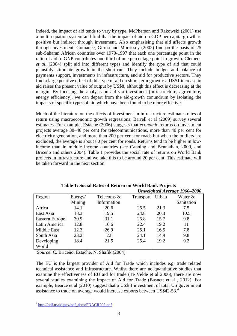
Much of the literature on the effects of investment in infrastructure estimates rates of

return using macroeconomic growth regressions. Barrell et al (2009) survey several

estimates. For example, Estache (2006) suggests that economic returns on investment

projects average 30–40 per cent for telecommunications, more than 40 per cent for

electricity generation, and more than 200 per cent for roads but when the outliers are

excluded, the average is about 80 per cent for roads. Returns tend to be higher in low-

income than in middle income countries (see Canning and Bennathan, 2000, and

Briceño and others 2004). Table 1 provides the social rate of returns on World Bank

projects in infrastructure and we take this to be around 20 per cent. This estimate will

be taken forward in the next section.

Table 1: Social Rates of Return on World Bank Projects

Unweighted Average 1960–2000

Region Energy/

Mining

Telecoms &

Information

Transport Urban Water &

Sanitation

Africa 14.1 20.6 25.5 21.3 7.5

East Asia 18.3 19.5 24.8 20.3 10.5

Eastern Europe 30.9 31.1 25.8 15.7 9.8

Latin America 12.8 16.6 22.4 19.2 11

Middle East 12.3 26.9 25.1 16.5 7.8

South Asia 23.2 22 24.1 14.9 9.8

Developing

World

18.4 21.5 25.4 19.2 9.2

Source: C. Briceño, Estache, N. Shafik (2004)

The EU is the largest provider of Aid for Trade which includes e.g. trade related

technical assistance and infrastructure. Whilst there are no quantitative studies that

examine the effectiveness of EU aid for trade (Te Velde et al 2006), there are now

several studies examining the impact of Aid for Trade (Basnett et al , 2012). For

example, Bearce et al (2010) suggest that a US$ 1 investment of total US government

assistance to trade on average would increase exports between US$42-53.4

4 http://pdf.usaid.gov/pdf_docs/PDACR202.pdf

9

Ferro et al (2011) examine the impact of aid for trade on the manufacturing and

services sectors. They find that a 10 per cent increase in aid to transportation, ICT,

energy, and banking services is associated with a 2 per cent, 0.3 per cent, 6.8 per cent,

and 4.7 per cent increase of manufacturing exports in receiving countries, respectively.

Aid to the business service sector is positive but not statistically significant. They also

include regional estimations, e.g. in Sub-Saharan Africa, aid to energy, ICT, and

banking had the largest statistically significant impacts on manufactured exports, with

a 10 per cent increase in aid associated with increases of manufactured exports of 6.37

per cent, 4.83 per cent, and 2.23 per cent, respectively (and greater than in most other

regions).

Cali and te Velde (2011) examine the impact of aid for trade and trade costs and

exports. They found that a US$1 million increase in aid for trade facilitation is

associated with a 6 per cent reduction in the cost of packing, loading, and shipping to

the transit hub. The estimations (column 4 of table 3 in their publication) find that the

elasticity of trade costs to increased aid for trade is significant with a value of around -

0.10. Taking this elasticity we can calculate that a 60 per cent increase in SSA aid

(which corresponds to the simulations in the next section) would lead to a decline of

around 6 per cent in the costs of exporting or importing.

2.3 EU aid and European performance

We live in an interdependent world and growth in developing countries is also good

for others. The benefits of faster growth in developing countries, in part due to EU aid

as per the previous section, are non-economic (less conflict and more stability, fewer

communicable diseases, etc.) but also economic. Emerging and developing economies

have been leading global growth for a decade (IMF, 2012) as shown in Figure 2. This

growth in the poorest countries has also stimulated demand and imports into their

economies. For example, EU27 exports to a sample of the 36 low income countries

increased by 125 per cent over the decade to 2010, equivalent to an additional US$12

billion (or €9.2 billion) of exports each year (UN Comtrade data).

Figure 2 Annual contribution to growth in world GDP per capita

(blue advanced economies; red emerging and developing economies)

Source : IMF World Economic Outlook October 2012

10

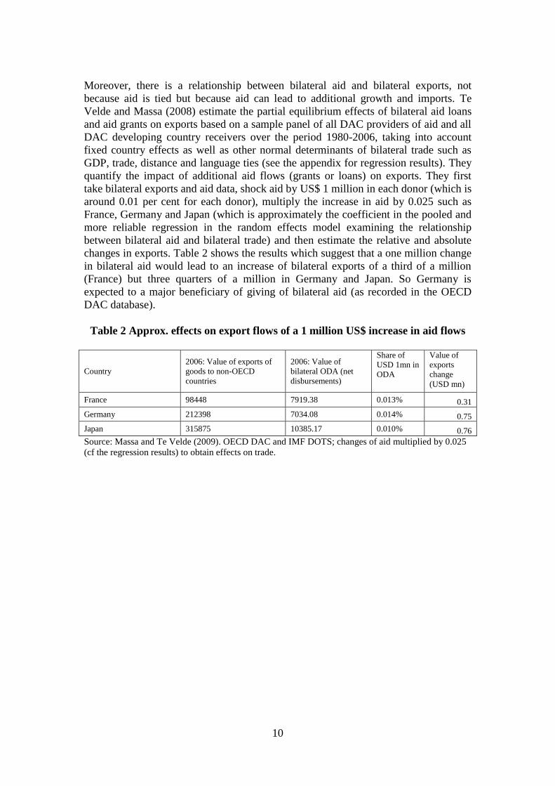
Moreover, there is a relationship between bilateral aid and bilateral exports, not

because aid is tied but because aid can lead to additional growth and imports. Te

Velde and Massa (2008) estimate the partial equilibrium effects of bilateral aid loans

and aid grants on exports based on a sample panel of all DAC providers of aid and all

DAC developing country receivers over the period 1980-2006, taking into account

fixed country effects as well as other normal determinants of bilateral trade such as

GDP, trade, distance and language ties (see the appendix for regression results). They

quantify the impact of additional aid flows (grants or loans) on exports. They first

take bilateral exports and aid data, shock aid by US$ 1 million in each donor (which is

around 0.01 per cent for each donor), multiply the increase in aid by 0.025 such as

France, Germany and Japan (which is approximately the coefficient in the pooled and

more reliable regression in the random effects model examining the relationship

between bilateral aid and bilateral trade) and then estimate the relative and absolute

changes in exports. Table 2 shows the results which suggest that a one million change

in bilateral aid would lead to an increase of bilateral exports of a third of a million

(France) but three quarters of a million in Germany and Japan. So Germany is

expected to a major beneficiary of giving of bilateral aid (as recorded in the OECD

DAC database).

Table 2 Approx. effects on export flows of a 1 million US$ increase in aid flows

Country

2006: Value of exports of

goods to non-OECD

countries

2006: Value of

bilateral ODA (net

disbursements)

Share of

USD 1mn in

ODA

Value of

exports

change

(USD mn)

France 98448 7919.38 0.013% 0.31

Germany 212398 7034.08 0.014% 0.75

Japan 315875 10385.17 0.010% 0.76

Source: Massa and Te Velde (2009). OECD DAC and IMF DOTS; changes of aid multiplied by 0.025

(cf the regression results) to obtain effects on trade.

11

3 Policy scenarios and model description

3.1 Simulating the effects of EU aid

In this section we assess the impact of EU aid through the EDF and DCI programmes

on both the donor and recipient countries. The analysis is carried out through a series

of model simulations, using the National Institute’s Global Econometric Model,

NiGEM. The NiGEM model has been in use at the National Institute for forecasting

and policy analysis since 1987, and is also used by a group of about 40 model

subscribers, mainly in the policy community, including the Bank of England, the

ECB, the OECD and the IMF. Most countries in the OECD are modelled separately,

and there are also separate models of China, India, Russia, Hong Kong, Taiwan,

Brazil, South Africa, Estonia, Latvia, Lithuania, Slovenia, Romania and Bulgaria. The

rest of the world is modelled through regional blocks so that the model is global in

scope5. The regional groups are consistent with IMF country groups, as defined for

the World Economic Outlook database, except that they exclude countries that are

modelled individually within NiGEM. Below we look at the impact of the flow of aid

to the regions defined as Sub-Saharan Africa, Latin America and the Caribbean,

Developing Asia and the Commonwealth of Independent States.

All country and regional models in NiGEM contain the determinants of domestic

demand, a supply side, export and import volumes, prices, current accounts and net

foreign assets. Output is determined in the long run by factor inputs and technical

progress interacting through production functions, but is driven by demand in the

short- to medium-term. Economies are linked through trade, competitiveness and

financial markets and are fully simultaneous. Further details on the NiGEM model are

available at http://nimodel.niesr.ac.uk/.

Foreign aid flows through the current accounts, with a negative effect on current

account balances in the donor countries and a positive effect on current account

balances in the recipient countries. This has implications for the accumulation of

foreign assets, as the size of the current account balance must equate to the change in

the net stock of foreign assets in each country (after allowing for any revaluation

effects). Aid recipients will see an improvement in their net foreign asset position,

while donors will see a deterioration. In US$ terms, the direct net rise in recipient

assets will roughly equal the direct net decline in donor net assets. However, if a large

economy sends aid to a smaller economy, the gains in the recipient country in

percentage terms would be high relative to the losses in the donor country. On top of

this, purchasing power matters. If €1 can buy more in the recipient country than it can

buy in the sending country, there is a net gain from the transfer at the global level,

even before allowing for any of the factors such as trade expansion that we explore

further below.

The aid must be financed from somewhere, and in the scenarios below we will

assume that the aid flows are financed by a temporary rise in government debt in the

donor countries, which must at some point be repaid. NiGEM operates with a tax rule

5 See Appendix A for details on the composition of regional groupings.

12

in place to ensure that governments remain solvent. Any rise in government debt will

induce an endogenous response in the rate of income tax, in order to bring the fiscal

position back in line with its target. This ensures that the deficit and debt stock return

to sustainable levels after a shock. This implies that aid outflows entail future income

tax liabilities, and so without allowing for any additional impacts through trade or

prices would have a negative impact on output in the donor economies. But later we

will have a more realistic picture that includes the effects of aid on other factors.

The impact of aid on both the recipient and donor countries depends on how the funds

are spent. If the funds are spent purely on paying down outstanding debt, there is little

impact on either country, as demonstrated by Barrell et al (2009). In the first scenario

we look at in the next section, we consider the impact of aid that is directed in this

way. This can be expected to have limited impact on trade and the full costs of the aid

flows will ultimately be borne by the taxpayer in the donor countries. However, we

will demonstrate that well-directed aid will entail little or no costs to the taxpayer, and

can even benefit taxpayers in the donor countries. If the funds are spent on current

consumption, such as supporting social safety nets, there will be a short-term stimulus

to demand in the recipient countries. This in turn will raise demand for imported

goods within the recipient, and so support exports from the rest of the world,

including the donor countries. This will offset and may outweigh the direct costs of

the aid to the donor countries.

If the aid is spent on productive investment, this will raise the available capital stock

within the recipient countries, and have a permanently positive effect on the level of

potential output, whereas when spending is spent purely on current consumption the

effects would be expected to largely dissipate within a few years of the transfer,

unless the rise in consumption stimulates domestic investment. If aid can be

channeled into productive investment, this will have a longer-lasting impact on output

in the recipient countries, although the short-term effects may not differ significantly

from spending on current consumption. The long-term rise in productive capacity in

the recipient countries will be more likely to have a positive impact on the donor

countries, who gain from a longer-term rise in exports to the recipient countries.

Some investment is more productive than others. Infrastructure investment has been

identified as one of the crucial areas towards which to direct aid, as the benefits to

both the recipients and donors are likely to be large. This raises the speed of the

adoption of technology from the advanced economies and reduces the costs of

distribution of all products, produced for both domestic and external markets. Briceno

et al (2004), for example, suggest a social rate of return on investment in transport

infrastructure of about 20 per cent in emerging and developing markets (see table 1

above). This means that in addition to the rise in the capital stock driven by the

investment, productivity on a broader level rises as well. Cali and te Velde (2009)

suggest that aid designated for trade facilitation can have a marked effect on trade

prices, reducing the costs of exports from the recipient countries. This raises the

competitiveness and demand for recipient exports and also reduces import costs for

the rest of the world. Trade facilitation can also reduce the import costs in the

recipient country of goods from the rest of the world, which should have a net positive

impact on world trade and global demand.

13

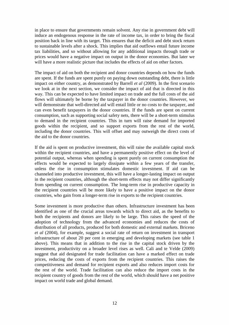
As discussed in section 2, our simulation studies are based on a flow of funds

channeled through the EDF and DCI programmes to Sub-Saharan Africa, Latin

America and the Caribbean, Developing Asia (incl. Pacific) and the Commonwealth

of Independent States. The total magnitude of the aid amounts to €51 billion, spread

evenly over the seven-year period. This equates to €3 billion per annum to Sub-

Saharan Africa, €2.1 billion per annum to Developing Asia (including Pacific), €0.7

billion per annum to the Commonwealth of Independent States and €1.4 billion per

annum to Latin America and the Caribbean. We assume that 40 per cent of the funds

are directed towards supporting current consumption and production, while 60 per

cent is directed towards social and economic infrastructure investment. Improved

infrastructure is expected to raise productivity, and we allow a 20 per cent social rate

of return on the investment in infrastructure (see section 2), introduced gradually over

the seven-year period.

We distribute the outflows across the donor countries, based on their share of total

contributions to the DCI in 2011 and the proposed future contributions to the EDF.

The share of the total €51 billion in aid flows that is attributed to each donor country

is illustrated in figure 3.

Figure 3. Share of EDF and DCI financed by each donor6

3.0%0.8%

1.0%1.2%1.4%1.6%1.6%

2.0%2.4%

2.7%2.9%

3.2%4.2%

9.0%12.3%

13.4%17.6%

19.7%

0.0% 2.0% 4.0% 6.0% 8.0% 10.0% 12.0% 14.0% 16.0% 18.0% 20.0%

OtherIreland

Czech RepHungaryPortugalFinlandGreece

DenmarkAustriaPoland

SwedenBelgium

NethsSpain

UK Italy

FranceGermany

Source: Authors calculations based on European Commission’s Financial Report

2011 and European Commission’s 2011 proposal for an internal agreement on the

11th European Development Fund.

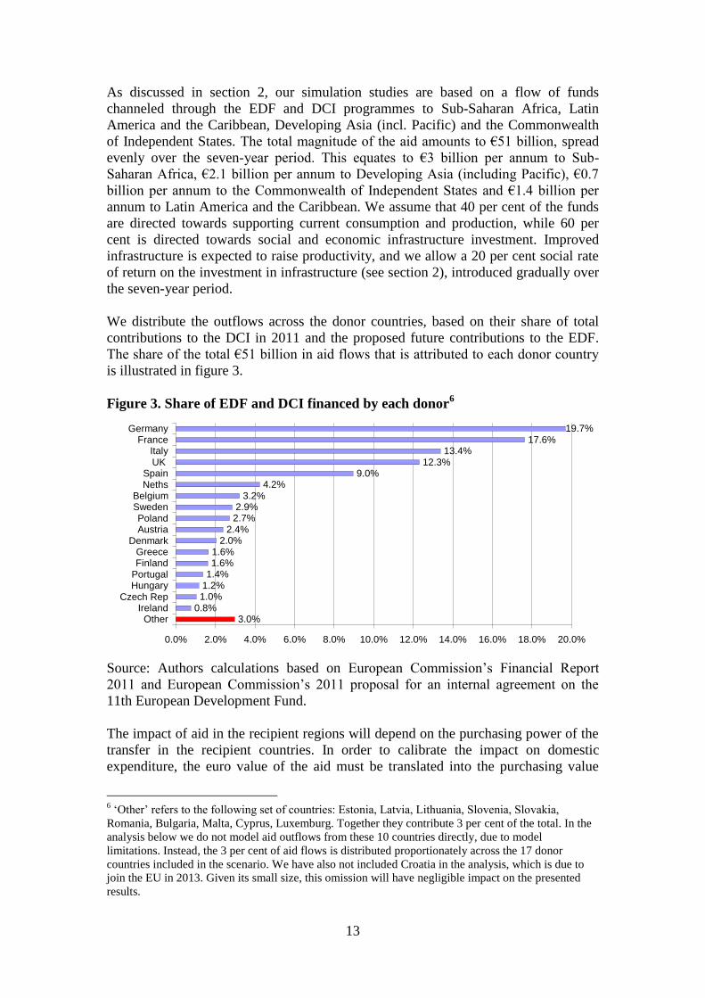
The impact of aid in the recipient regions will depend on the purchasing power of the

transfer in the recipient countries. In order to calibrate the impact on domestic

expenditure, the euro value of the aid must be translated into the purchasing value

6 ‘Other’ refers to the following set of countries: Estonia, Latvia, Lithuania, Slovenia, Slovakia,

Romania, Bulgaria, Malta, Cyprus, Luxemburg. Together they contribute 3 per cent of the total. In the

analysis below we do not model aid outflows from these 10 countries directly, due to model

limitations. Instead, the 3 per cent of aid flows is distributed proportionately across the 17 donor

countries included in the scenario. We have also not included Croatia in the analysis, which is due to

join the EU in 2013. Given its small size, this omission will have negligible impact on the presented

results.

14

within the recipients. The conversion is calculated using the 2005 ratio of GDP in

purchasing power parity (PPP) exchange rates to GDP in current US$ in each region,

from the IMF WEO database. This ratio is illustrated in figure 4. The figure shows

that €1 is worth at least €2 in the recipient countries, and up to €2.8 in the Developing

Asia region. This suggests that there are substantial gains to be made at the global

level from transfers from the EU to developing and emerging economies simply due

to the purchasing power effects. As we illustrate below, these positive effects are

strengthened through enhanced trade and productivity developments.

Figure 4 Purchasing power parity relative to euro exchange rate

1

1.2

1.4

1.6

1.8

2

2.2

2.4

2.6

2.8

3

SSA CIS Asia Lat Am

PPP/€

Source: Derived from IMF World Economic Outlook database

In order to calibrate the impact of investment on the long-run capacity of the region to

produce, we need to consider two channels. The first is the contribution to the capital

stock. This requires an initial assumption as to the quantity of existing capital in each

region and an estimate of the expected rate of depreciation of the investment. The

second is the expected “social rate of return” on the investment, or the spillovers to

the rest of the economy through reduced distribution costs and the like.

We base our estimate of the initial magnitude of the existing capital stock in each

recipient region broadly on the estimates reported in Nehru and Dhareshwar (1993).

This points to a capital output ratio averaging 2.6 in Sub-Saharan Africa, 2.8 in

Developing Asia and 3.0 in the Commonwealth of Independent States and the Latin

America and the Caribbean region. We assume a 10 per cent rate of depreciation per

annum of the new investment. While this is somewhat lower than estimates reported

by some studies, such as Bu (2006), it is higher than usual estimates for the rate of

depreciation for advanced economies. Given these assumptions, and an estimate that

60 per cent of the aid will be directed towards investment (the sum of social and

economic infrastructure, see section 2), this allows us to calculate the impact of

capital accumulation on the potential level of output in each recipient region.

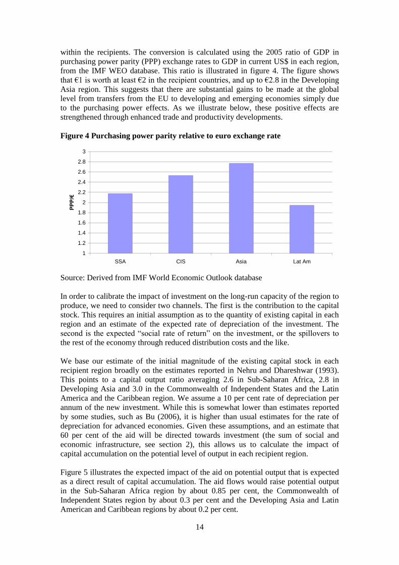
Figure 5 illustrates the expected impact of the aid on potential output that is expected

as a direct result of capital accumulation. The aid flows would raise potential output

in the Sub-Saharan Africa region by about 0.85 per cent, the Commonwealth of

Independent States region by about 0.3 per cent and the Developing Asia and Latin

American and Caribbean regions by about 0.2 per cent.

15

Figure 5 Impact of capital accumulation on potential output

0.00

0.10

0.20

0.30

0.40

0.50

0.60

0.70

0.80

0.90

2014 2015 2016 2017 2018 2019 2020 2021 2022 2023 2024 2025 2026 2027

pe

r c

en

t d

iffe

ren

ce

fro

m b

as

e

SSA CIS Dev Asia Lat Am

We estimate that the investment has a 20 per cent social rate of return, a conservative

estimate in line with rates reported by, for example, Briceno et al (2004). This means

that the direct effects of capital accumulation on potential output in each region,

illustrated in figure 5, are augmented by a further 20 per cent through productivity

gains. Based on this assumption, trend productivity is expected to rise by 0.17 per

cent in Sub-Saharan Africa, by 0.06 per cent in the Commonwealth of Independent

States and 0.04 per cent in Developing Asia and Latin America and the Caribbean7.

This is implemented as a gradual rise over the seven-year period.

Cali and te Velde (2009, 2011) demonstrate that investment directed towards trade

facilitation can significantly reduce the costs of trading with the recipient regions.

Based on their estimates, if the aid flows are directed towards infrastructure

investments that facilitate trade, this would be expected to reduce export prices from

Sub-Saharan Africa by about 6 per cent over the seven-year period. Using this as a

benchmark figure, we calibrate export price declines in the other regions by assessing

the magnitude of the planned aid inflow relative to total exports from each region.

This implies a 2 per cent decline in export prices from the Commonwealth of

Independent States, a 1.3 per cent decline in export prices from Latin America and the

Caribbean and a 1 per cent decline in export prices from Developing Asia.

Trade facilitation should also mean that exporting to the aid recipient regions becomes

less expensive. We calibrate the implied decline in export prices from the EU

countries according to their share of exports directed towards each of the aid recipient

regions. Figure 6 illustrates the expected decline in export prices relative to baseline

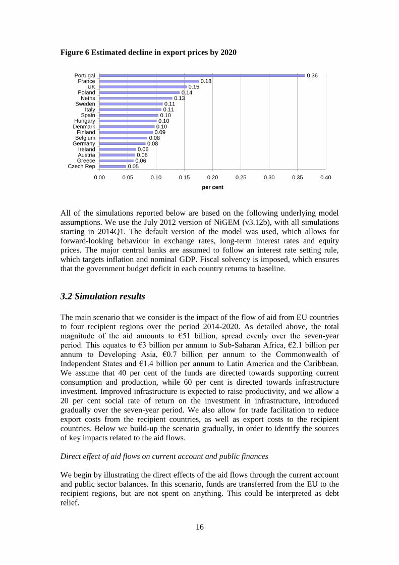
in each of the EU donor countries included in the scenario. Portugal stands out as

expecting the most significant decline in trade prices, due to the high share of exports

sent to the regions. Portugal sends more than 5 per cent of its total exports to Sub-

Saharan Africa and more than 2 per cent to Developing Asia. The Czech Republic,

Greece, Austria and Ireland, on the other hand, conduct relatively little trade with the

regions, and have less to gain in terms of trade facilitation.

7 This is simply calibrated as 20 per cent of the estimated rise in the capital stock in each region.

16

Figure 6 Estimated decline in export prices by 2020

0.050.060.060.06

0.080.08

0.090.100.100.10

0.110.11

0.130.14

0.150.18

0.36

0.00 0.05 0.10 0.15 0.20 0.25 0.30 0.35 0.40

Czech RepGreeceAustriaIreland

GermanyBelgiumFinland

DenmarkHungary

SpainItaly

SwedenNeths

PolandUK

FrancePortugal

per cent

All of the simulations reported below are based on the following underlying model

assumptions. We use the July 2012 version of NiGEM (v3.12b), with all simulations

starting in 2014Q1. The default version of the model was used, which allows for

forward-looking behaviour in exchange rates, long-term interest rates and equity

prices. The major central banks are assumed to follow an interest rate setting rule,

which targets inflation and nominal GDP. Fiscal solvency is imposed, which ensures

that the government budget deficit in each country returns to baseline.

3.2 Simulation results

The main scenario that we consider is the impact of the flow of aid from EU countries

to four recipient regions over the period 2014-2020. As detailed above, the total

magnitude of the aid amounts to €51 billion, spread evenly over the seven-year

period. This equates to €3 billion per annum to Sub-Saharan Africa, €2.1 billion per

annum to Developing Asia, €0.7 billion per annum to the Commonwealth of

Independent States and €1.4 billion per annum to Latin America and the Caribbean.

We assume that 40 per cent of the funds are directed towards supporting current

consumption and production, while 60 per cent is directed towards infrastructure

investment. Improved infrastructure is expected to raise productivity, and we allow a

20 per cent social rate of return on the investment in infrastructure, introduced

gradually over the seven-year period. We also allow for trade facilitation to reduce

export costs from the recipient countries, as well as export costs to the recipient

countries. Below we build-up the scenario gradually, in order to identify the sources

of key impacts related to the aid flows.

Direct effect of aid flows on current account and public finances

We begin by illustrating the direct effects of the aid flows through the current account

and public sector balances. In this scenario, funds are transferred from the EU to the

recipient regions, but are not spent on anything. This could be interpreted as debt

relief.

17

As illustrated in figure 7, the current account balances in the recipient regions

improve slightly (by up to 0.1 per cent of GDP), while there is a small worsening of

balances within the donor region. This is matched by a modest accumulation of net

foreign assets in the recipients, reaching 0.4 per cent of GDP in Sub-Saharan Africa

by 2020 with small impacts elsewhere.

Figure 7 Impact of aid flows on current account balances (% of GDP)

-0.08

-0.06

-0.04

-0.02

0.00

0.02

0.04

0.06

0.08

0.10

0.12

0.14

2014 2015 2016 2017 2018 2019

Ab

so

lute

diffe

ren

ce

fro

m b

ase

SSA Dev Asia CIS Lat Am Euro Area

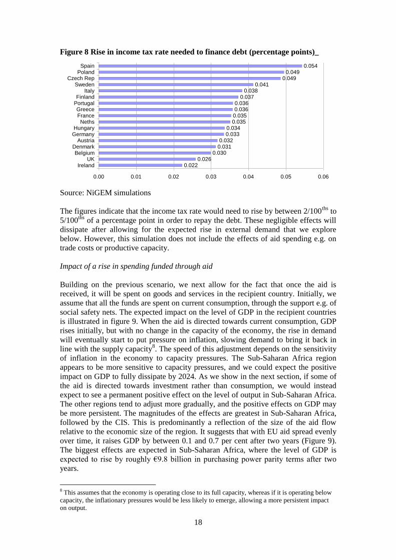
If the aid is financed by issuing government debt, this must be repaid at some point in

the future. We assume that this repayment is effected through income taxes. Figure 8

illustrates the estimated rise in the income tax rate by 2020 that would be needed in

each country to pay back this debt. The rise would be temporary and would dissipate

over the next few years as the debt is repaid. This is based on the assumption that the

aid is directed simply towards paying off existing debt of the recipient countries. Aid

directed in this way can be expected to have limited impact on trade and the full costs

of the aid flows will ultimately be borne by the taxpayer in the donor countries.

However, we will demonstrate below that well-directed aid will entail little or no

costs to the taxpayer, and is even expected to benefit taxpayers in the donor countries.

18

Figure 8 Rise in income tax rate needed to finance debt (percentage points)_

0.0220.026

0.0300.0310.032

0.0330.034

0.0350.0350.0360.036

0.0370.038

0.0410.049

0.0490.054

0.00 0.01 0.02 0.03 0.04 0.05 0.06

IrelandUK

BelgiumDenmark

AustriaGermanyHungary

NethsFranceGreece

PortugalFinland

ItalySweden

Czech RepPoland

Spain

Source: NiGEM simulations

The figures indicate that the income tax rate would need to rise by between 2/100ths

to

5/100ths

of a percentage point in order to repay the debt. These negligible effects will

dissipate after allowing for the expected rise in external demand that we explore

below. However, this simulation does not include the effects of aid spending e.g. on

trade costs or productive capacity.

Impact of a rise in spending funded through aid

Building on the previous scenario, we next allow for the fact that once the aid is

received, it will be spent on goods and services in the recipient country. Initially, we

assume that all the funds are spent on current consumption, through the support e.g. of

social safety nets. The expected impact on the level of GDP in the recipient countries

is illustrated in figure 9. When the aid is directed towards current consumption, GDP

rises initially, but with no change in the capacity of the economy, the rise in demand

will eventually start to put pressure on inflation, slowing demand to bring it back in

line with the supply capacity8. The speed of this adjustment depends on the sensitivity

of inflation in the economy to capacity pressures. The Sub-Saharan Africa region

appears to be more sensitive to capacity pressures, and we could expect the positive

impact on GDP to fully dissipate by 2024. As we show in the next section, if some of

the aid is directed towards investment rather than consumption, we would instead

expect to see a permanent positive effect on the level of output in Sub-Saharan Africa.

The other regions tend to adjust more gradually, and the positive effects on GDP may

be more persistent. The magnitudes of the effects are greatest in Sub-Saharan Africa,

followed by the CIS. This is predominantly a reflection of the size of the aid flow

relative to the economic size of the region. It suggests that with EU aid spread evenly

over time, it raises GDP by between 0.1 and 0.7 per cent after two years (Figure 9).

The biggest effects are expected in Sub-Saharan Africa, where the level of GDP is

expected to rise by roughly €9.8 billion in purchasing power parity terms after two

years.

8 This assumes that the economy is operating close to its full capacity, whereas if it is operating below

capacity, the inflationary pressures would be less likely to emerge, allowing a more persistent impact

on output.

19

Figure 9 Impact of aid spent on current consumption on GDP in recipients

0

0.1

0.2

0.3

0.4

0.5

0.6

0.7

0.8

0.9

2014 2015 2016 2017 2018 2019 2020

% d

iffe

ren

ce

fro

m b

ase

SSA CIS Asia Lat Am

Source: NiGEM simulations.

Note: Figure illustrates the expected impact on the level of GDP, accumulating the

effects of aid flows over time.

Directing spending towards infrastructure investment

As the next stage in building our scenario, we designate 60 per cent of the aid flows to

be directed towards economic and social infrastructure investment in the recipient

regions, while the remaining 40 per cent is directed towards current consumption. As

we discussed in the previous section, investment in infrastructure can affect the

productive capacity of the economy through two channels: a direct effect through the

increase in the stock of infrastructure capital in the economy, and an indirect effect

through productivity spillovers to the rest of the economy, as an improved

infrastructure allows trade in all goods and services to be conducted more rapidly and

efficiently. We assume a 20 per cent rate of return on the investment in infrastructure

(see section 2.2).

Figure 10 Impact on GDP, of aid with 60% directed towards infrastructure

0

0.2

0.4

0.6

0.8

1

1.2

2014 2015 2016 2017 2018 2019 2020 2021 2022 2023 2024 2025 2026 2027

% d

iffe

ren

ce

fro

m b

ase

SSA CIS Asia Lat Am

20

When we allow for aid to be directed towards infrastructure investment, the level of

GDP remains permanently above base in all regions. The biggest impact is in Sub-

Saharan Africa, where the magnitude of aid flows is highest.

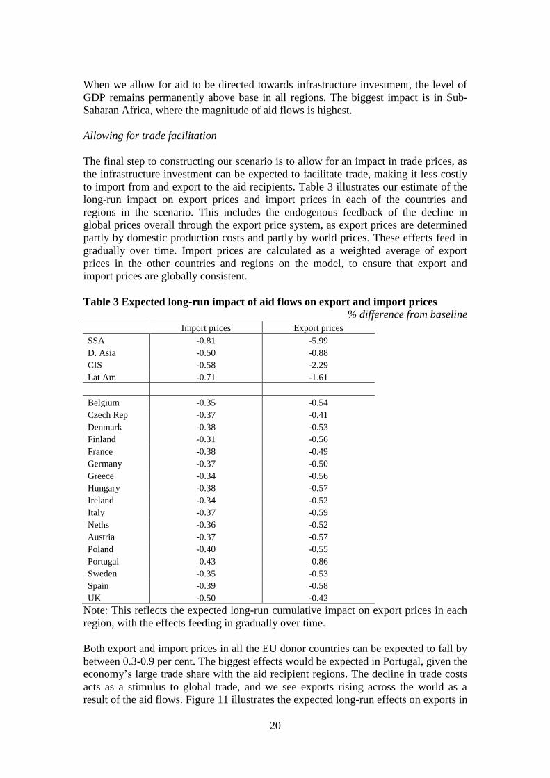
Allowing for trade facilitation

The final step to constructing our scenario is to allow for an impact in trade prices, as

the infrastructure investment can be expected to facilitate trade, making it less costly

to import from and export to the aid recipients. Table 3 illustrates our estimate of the

long-run impact on export prices and import prices in each of the countries and

regions in the scenario. This includes the endogenous feedback of the decline in

global prices overall through the export price system, as export prices are determined

partly by domestic production costs and partly by world prices. These effects feed in

gradually over time. Import prices are calculated as a weighted average of export

prices in the other countries and regions on the model, to ensure that export and

import prices are globally consistent.

Table 3 Expected long-run impact of aid flows on export and import prices

% difference from baseline

Import prices Export prices

SSA -0.81 -5.99

D. Asia -0.50 -0.88

CIS -0.58 -2.29

Lat Am -0.71 -1.61

Belgium -0.35 -0.54

Czech Rep -0.37 -0.41

Denmark -0.38 -0.53

Finland -0.31 -0.56

France -0.38 -0.49

Germany -0.37 -0.50

Greece -0.34 -0.56

Hungary -0.38 -0.57

Ireland -0.34 -0.52

Italy -0.37 -0.59

Neths -0.36 -0.52

Austria -0.37 -0.57

Poland -0.40 -0.55

Portugal -0.43 -0.86

Sweden -0.35 -0.53

Spain -0.39 -0.58

UK -0.50 -0.42

Note: This reflects the expected long-run cumulative impact on export prices in each

region, with the effects feeding in gradually over time.

Both export and import prices in all the EU donor countries can be expected to fall by

between 0.3-0.9 per cent. The biggest effects would be expected in Portugal, given the

economy’s large trade share with the aid recipient regions. The decline in trade costs

acts as a stimulus to global trade, and we see exports rising across the world as a

result of the aid flows. Figure 11 illustrates the expected long-run effects on exports in

21

the EU and the world as a whole. By 2020, the value of world trade would be

expected to rise by €120 billion as a result of the aid flows.

Figure 11 Expected long-run impact of aid flows on export volumes

0.910.71

0.600.600.620.630.64

0.660.710.710.720.730.730.750.780.790.790.80

1.57

0.00 0.20 0.40 0.60 0.80 1.00 1.20 1.40 1.60 1.80

WorldEU

GreeceAustria

Czech RepGermany

IrelandFinland

UKSweden

DenmarkPoland

ItlanyBelgium

NethsFrance

SpainHungaryPortugal

% difference from base

Figure 12 illustrates the expected impact of the aid flows on GDP in the recipient

regions. The impact on Sub-Saharan Africa is expected to be significantly greater than

the other regions, as the magnitude of the flows is higher relative to both the size of

the economy and relative to the level of total exports from the region. After 10 years,

we would expect the level of output in Sub-Saharan Africa to be 2½ per cent higher

than it would be without the aid – or more than €55 billion by 2024. Output in the

other regions would be expected to rise by ¼ - ¾ per cent after 10 years. At the global

level, output is expected to be 0.2 per cent higher by 2020 as a result of the

programme, reflecting the cumulative effects in both recipient and donor countries, as

well as the rest of the world. The impact that this would be expected to have on global

employment depends on the global income elasticity of employment, the degree of

concurrent productivity gains and the response of real wages to declines in

unemployment, but would be expected to lie in the range of 600,000-3,000,000 jobs

worldwide.

Figure 12 Expected impact of aid flows on GDP in recipient regions

0

0.5

1

1.5

2

2.5

3

2014 2015 2016 2017 2018 2019 2020 2021 2022 2023 2024 2025 2026 2027

% d

iffe

ren

ce

fro

m b

ase

SSA CIS Asia Lat Am

22

In the donor countries, we would also expect output to be higher as a result of the aid

flows. Figure 13 illustrates the expected impact on the level of output in each of the

donor countries at the end of the seven-year period. While the effects are small, the

gains from the rise in trade and decline in trade costs are expected to outweigh the

losses due to the deterioration of current account balances and rise in tax needed to

finance the aid. At the EU-wide level, we expect the level of output to be 0.09 per

cent higher by 2020 as a result of the aid programme, or €11.5 billion. Within the EU,

the biggest impacts on GDP are expected to materialise in Portugal and Hungary, with

smaller impacts expected in the UK and Germany. The total aid flows from the EU of

€51 billion amount to approximately 0.4 per cent of the projected level of EU GDP

for 2013. These costs are more than compensated for by the expected gains in trade

and cost reductions, with more than a 20 per cent return on the investment.

Figure 13 Expected impact on GDP in donor countries and world, 2020

0.0310.040

0.0590.0690.072

0.0790.1000.102

0.1060.113

0.1220.130

0.1650.1750.177

0.2120.276

0.0860.222

0.00 0.05 0.10 0.15 0.20 0.25 0.30

UKGermany

IrelandGreece

SwedenAustria

DenmarkSpain

FranceItaly

Czech RepFinland

BelgiumNeths

PolandHungaryPortugal

EU World

per cent difference from base

Figure 14 illustrates the expected impact on the income tax rate in each country as a

result of the policy. The effects differ markedly from those illustrated in the first

scenario above, as the anticipated rise in GDP supports public finances, and in more

than half of the countries we would expect tax rates to actually decline as a result of

the aid flows, despite the initial rise in government debt required to finance the aid. In

the remaining countries, the expected rise in income tax rates is negligible, with a

maximum increase of 18/1000’s of a percentage point needed in Hungary and the

Czech Republic. If the average income is €25,000 per annum, this would imply a rise

in the average tax burden of just €4.5 per annum. Over the 7 years of the investment

even these costs are offset by the rise in trade and reductions in consumer prices, and

the investment made in the €51bn in development aid is completely recouped by EU

taxpayers.

23

Figure 14 Expected impact on income tax rates in donor countries, 2020

(percentage points)

-0.042-0.026

-0.023-0.013

-0.011-0.004-0.003-0.002

-0.0010.002

0.0110.012

0.0130.0170.0170.0180.018

-0.05 -0.04 -0.03 -0.02 -0.01 0.00 0.01 0.02 0.03

BelgiumPortugal

NethsFranceFinland

ItlanyGermany

UKDenmark

PolandSwedenIrelandAustria

SpainGreeceCzech

Hungary

4 Conclusions

This paper examined the quantitative effects of EU aid (specifically the European

Development Fund and the Development Cooperation Instrument totalling €51 billion

over 2014-2020). This is the first study that quantifies the potential effects of

proposed EU aid on both sending and receiving countries. We reviewed the literature

on EU aid and the effects of aid generally, used this to derive possible effects of EU

aid which are subsequently modelled in a commonly used general equilibrium model.

If managed well, EU aid can lead to faster growth in receiving countries which will

lead to faster growth in imports including from the EU. This paper shows that under

certain plausible assumptions, EU aid is an investment that can lead to positive net

effects on growth in the EU. We estimate a 20 per cent return on the investment in

developing countries if aid is channelled effectively. By 2020, this €51bn aid

investment will lead to an almost 0.1 per cent boost in European GDP, a 0.2 per cent

boost to global GDP and global gains in employment which are expected to fall

within the range of 600,000-3,000,000. The net cost to the EU citizen of this

investment would be zero, and the boost in growth will mean a positive net gain for

the EU, as well as for the recipient countries.

24

References

Arndt, C., Jones, S. and Tarp, F. (2009), ‘Aid and Growth: Have We Come Full

Circle?’ WIDER Discussion Paper No. 2009/05.

Barrell, R., Holland, D., D.W. te Velde, (Mar 2009), A fiscal stimulus to address the

effects of the global financial crisis on sub-Saharan Africa, Dp. 331

Basnett, Y., Engel, J., Kennan, Kingombe, C., Massa, I., te Velde, D. W. (2012).

Increasing the effectiveness of Aid for Trade: the circumstances under which it

works best. Working Paper 353, London: Overseas Development Institute.

http://www.odi.org.uk/resources/details.asp?id=6771&title=increasing-

effectiveness-aid-trade

Birdsall, N. And Kharas, H. with Mahgoub, A. and Perakis, R. (2010) Quality of

Official Development Assistance Assessment

http://www.cgdev.org/files/1424481_file_CGD_QuODA_web.pdf

Bourguignon, F. and M. Sundberg (2007), Aid Effectiveness – Opening the Black

Box, American Economic Review P&P, 97(2) pp. 316-321

Bu, Y. (2006), ‘Fixed capital stock depreciation in developing countries: Some

evidence from firm-level data’, Journal of Development Studies, Vol. 42(5), pp.

881-901.

Briceno-Garmendia, C., A. Estache Antonio and Shafik, Nemat, Infrastructure

Services in Developing Countries: Access, Quality, Costs, and Policy Reform

(December 2004). World Bank Policy Research Paper No. 3468

Cali, M. and D.W. te Velde (2009), “Towards a quantitative assessment of aid for

trade”, Commonwealth Economic Paper

Cali, M. D.W. te Velde (2011), “Does aid for trade really improve trade

performance?” World Development

Canning, D. and E. Bennathan (2000), “The Social Rate of Return on Infrastructure

Investments”, World Bank Policy Research Working Paper No. 2390

Clemens, M., S. Radelet, and R. Bhavnani (2004), “Counting Chickens When They

Hatch: The Short-term Effect of Aid on Growth” CGD Working Paper 44

Doucouliagos, H., and M. Paldam (2007).The Aid Effectiveness Literature. The Sad

Result of 40 Years of Research, University of Aarhus, Department of Economics

Working Paper 2007-15.

Estache (2006), Infrastructure: A survey of recent and upcoming issues, World Bank

draft.

Ferro, E., A. Portugal-Perez, and J. S. Wilson, (2012), Aid to the Services Sector

Does It Affect Manufacturing Exports? WB paper 5728, http://www-

wds.worldbank.org/external/default/WDSContentServer/IW3P/IB/2011/07/19/000

158349_20110719152138/Rendered/PDF/WPS5728.pdf

Gomanee, K., S. Girma and O. Morrissey (2002), ‘Aid, Investment and Growth in

Sub-Saharan Africa’, paper prepared for the 10th General Conference of EADI,

Ljubljana, in Journal of International Development.

Hansen, H. and F. Tarp (2001), Aid and growth regressions, Journal of Development

Economics 64, pp. 547-70.

Massa, I. and D.W. te Velde (2009), “The trade distortion implications of loans and

grants”, paper for KfW.

McPherson, M.F. and T. Rakovski (2001), ‘Understanding the Growth Process in

Sub-Saharan Africa: Some Empirical Estimates’, African Economic Policy

Discussion Paper,

25

Nehru, V. and Dhareshwar, A. (1993), ‘A new database on physical capital stock:

sources, methodology and results’, Revista de Análisís Económica, Vol. 8(1), pp.

37-59.

Rajan, R.G. and A. Subramanian (2005), What Undermines Aid’s Impact on

Growth?, NBER Working Paper No. 11657.

Rajan, R.G., and A. Subramanian (2007), Aid and Growth: What Does the Cross-

Country Evidence Really Show, Review of Economics and Statistics

Rajan, R.G., and A. Subramanian, (2011). Aid, Dutch disease, and manufacturing

growth. Journal of Development Economics, 94 (1), pp. 106-118.

Tarp, F. (2012), Aid effectiveness, http://www.wider.unu.edu/publications/working-

papers/discussion-papers/2009/en_GB/dp2009-05/

World Bank (2006) Review of Selected Railway Concessions in Sub-Saharan Africa,

http://www4.worldbank.org/afr/ssatp/Resources/WorldBank-

WorkingPapers/ESW-RailwayConcessions.pdf

26

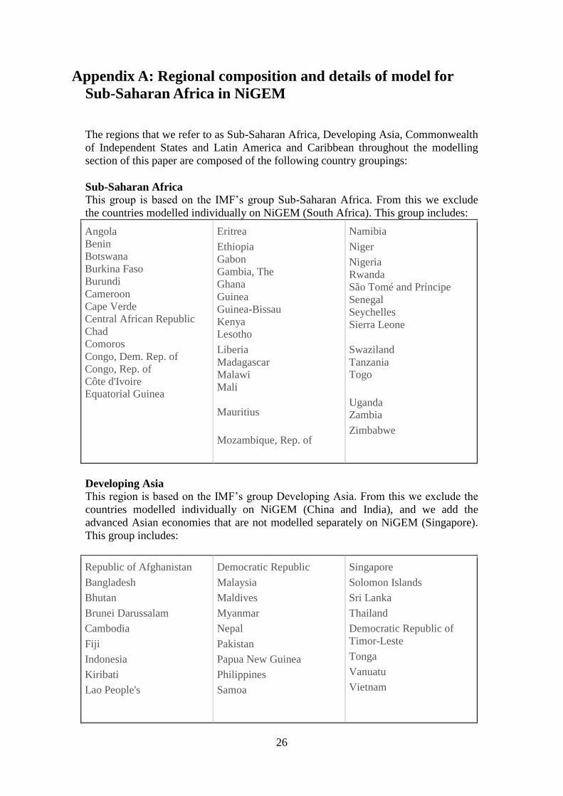
Appendix A: Regional composition and details of model for

Sub-Saharan Africa in NiGEM

The regions that we refer to as Sub-Saharan Africa, Developing Asia, Commonwealth

of Independent States and Latin America and Caribbean throughout the modelling

section of this paper are composed of the following country groupings:

Sub-Saharan Africa

This group is based on the IMF’s group Sub-Saharan Africa. From this we exclude

the countries modelled individually on NiGEM (South Africa). This group includes:

Angola

Benin

Botswana

Burkina Faso

Burundi

Cameroon

Cape Verde

Central African Republic

Chad

Comoros

Congo, Dem. Rep. of

Congo, Rep. of

Côte d'Ivoire Equatorial Guinea

Eritrea

Ethiopia

Gabon

Gambia, The

Ghana

Guinea

Guinea-Bissau

Kenya Lesotho

Liberia

Madagascar

Malawi

Mali

Mauritius

Mozambique, Rep. of

Namibia

Niger

Nigeria

Rwanda

São Tomé and Príncipe

Senegal

Seychelles

Sierra Leone

Swaziland

Tanzania Togo

Uganda Zambia

Zimbabwe

Developing Asia

This region is based on the IMF’s group Developing Asia. From this we exclude the

countries modelled individually on NiGEM (China and India), and we add the

advanced Asian economies that are not modelled separately on NiGEM (Singapore).

This group includes:

Republic of Afghanistan

Bangladesh

Bhutan

Brunei Darussalam

Cambodia

Fiji

Indonesia

Kiribati

Lao People's

Democratic Republic

Malaysia

Maldives

Myanmar

Nepal

Pakistan

Papua New Guinea

Philippines

Samoa

Singapore

Solomon Islands

Sri Lanka

Thailand

Democratic Republic of

Timor-Leste

Tonga

Vanuatu

Vietnam

27

Commonwealth of Independent States

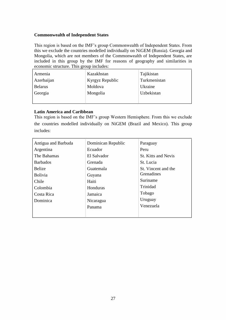
This region is based on the IMF’s group Commonwealth of Independent States. From

this we exclude the countries modelled individually on NiGEM (Russia). Georgia and

Mongolia, which are not members of the Commonwealth of Independent States, are

included in this group by the IMF for reasons of geography and similarities in

economic structure. This group includes:

Armenia

Azerbaijan

Belarus

Georgia

Kazakhstan

Kyrgyz Republic

Moldova

Mongolia

Tajikistan

Turkmenistan

Ukraine

Uzbekistan

Latin America and Caribbean

This region is based on the IMF’s group Western Hemisphere. From this we exclude

the countries modelled individually on NiGEM (Brazil and Mexico). This group

includes:

Antigua and Barbuda

Argentina

The Bahamas

Barbados

Belize

Bolivia

Chile

Colombia

Costa Rica

Dominica

Dominican Republic

Ecuador

El Salvador

Grenada

Guatemala

Guyana

Haiti

Honduras

Jamaica

Nicaragua

Panama

Paraguay

Peru

St. Kitts and Nevis

St. Lucia

St. Vincent and the

Grenadines

Suriname

Trinidad

Tobago

Uruguay

Venezuela

28

The key equations for the models of Sub-Saharan Africa are described below. The

other regional groups have models based on the same basic structure, although the

parameters are region specific.

AFCBV Current balance, US$ Mn

#i afcbv= afbpt+afxval -afmval+afipdc-afipdd

where afbpt are balance of payment transfers, afxval is African exports in US$, afmval is African

imports in US$, afipdc is interest payments received by Africa, afipdd is interest payments paid by

Africa.

AFPXCOM Price of commodity exports, US$, 2000=100

# afpxcom = 0.04873*wdpmm + 0.251114*wdpanf +

#0.042418*wdpfdv+0.32965*wdpfld

# + 0.328086*wdpo

where wdpmm is the price of metals and minerals, wdpanf is the price of agricultural non-foods,

wdpfdv is the price of food, wdpfld is the price of beverages and wdpo is the price of oil.

AFPXNCOM Price of non-commodity exports, US$, 2000=100

# log(afpxncom)= log(afpxncom(-1)) + 0.136269

# - 0.173991*(log(afpxncom(-1)) - 0.442582*log(afcpx(-1))

# - (1.-0.442582)* log(afcedd(-1)))

# + 0.105890* log(afpxncom(-1)/afpxncom(-2))

# + (1.-0.105890)* log(afcpx(-1)/afcpx(-2))

where afcpx is competitor’s export prices, afcedd is domestic prices in US$ terms.

AFPX Deflator, exports of goods and serv, US$, 2000=100

#i afpx = 0.27694*afpxcom + (1.-0.27694)*afpxncom

AFDD Domestic demand, US$ Bn, 2000 prices

# log(afdd) = log(afdd(-1))

# + 0.451 - 0.132189*(log(afdd(-1))

# - 0.60*log(afxvold(-1))

# + 0.0059783*afnar(-1))

# + 0.5*log(afpopt/afpopt(-1))

where afxvold is African export volumes in terms of domestic consumer prices, afnar is net foreign

debt as a share of GDP, and afpopt is total population.

AFMVOL Imports of goods and servs, Bn US$, 2000 prices

# log(afmvol)= log(afmvol(-1))- 0.284631

# - 0.092493*(log(afmvol(-1)) + 0.68077*log(afrpm(-1))

29

# - 1.24*log(afdd(-1)+afxvol(-1)))

# + 1.1*log((afdd+afxvol)/(afdd(-1)+afxvol(-1)))

# -0.06147*log(afrpm/afrpm(-1))

where afrpm is import prices relative to domestic prices.

AFXVOL Exports of goods and servs, Bn US$, 2000 prices

# log(afxvol) = log(afxvol(-1)) +0.11185

# -0.172654*(log(afxvol(-1)) +1.350605*log(afrpx(-1))

# -1.0*log(afs(-1)) )

# +1.08*log(afs/afs(-1)) -0.268*log((afrpx)/(afrpx(-1)))

where afrpx is African export prices relative to competitor’s, afs is external demand.

AFY GDP, US$ Bn, 2000 PPP

#i afy = afdd + afxvol - afmvol

AFCED Consumer expenditure deflator, 2000=100

# log(afced)= log(afced(-1))+ 0.001774

# -0.02545*(log(afced(-1))-log(afpmd(-1))-1.490*afog(-1))

# + 0.201981*log(afpmd/afpmd(-1))

# + 0.106133*log(afpmd(-1)/afpmd(-2))

# + (1.-0.201981-0.106133)*log(afinf)

# +0.22897*(afog-afog(-1))

where afpmd is import prices in domestic currency, afog is the output gap (afy/afycap), afinf is

inflation expectations.

AFYCAP Trend output for capacity utilisation

# log(afycap) = log(afycap(-1)) - 1.566 - 0.2*(log(afycap(-1)) - aftechl

# - log(afpopt(-1)) )

where aftechl is the level of technical progress and afpopt is total population.