the effect of food-away-from-home and food-at-home expenditures on

The Effect of Food-Away-from-Home and

Food-at-Home Expenditures on Obesity Rates:

A State-Level Analysis

Yongxia Cai, Pedro A. Alviola, IV, Rodolfo M. Nayga, Jr., and Ximing Wu

Using state-level data from the Behavioral Risk Factor Surveillance System, we investigate

the effects of household food-away-from-home and food-at-home expenditures on

overweight rates, obesity rates, and combined rates. Our random effects model estimates

suggest that food-away-from-home expenditures are positively related to obesity and

combined rates, while food-at-home expenditures are negatively related to obesity and

combined rates. However, the magnitudes of these effects, while statistically significant, are

relatively small. Both food-at-home and food-away-from-home expenditures do not

significantly influence overweight rates.

Key Words: food-at-home expenditures, food-away-from-home expenditures, obesity,

overweight, random effects model, state-level analysis

JEL Classifications: I18

Recent evidence has shown that obesity rates

have been increasing in the United States.

Both national-level data from the National

Health and Nutrition Examination Survey

(NHANES) and state-level data from the

Behavioral Risk Factor Surveillance System

(BRFSS) indicate that the prevalence of

obesity among adults continued to increase

during the past decade. According to BRFSS,

approximately 23.9% of U.S. adults in 2005

were obese, and the prevalence of obesity has

increased in all states during the period 1995–

2005 (Figure 1). Obesity is the second most

important cause of premature death, and it

increases the risk of many diseases, such as

hypertension, dyslipidemia, type 2 diabetes,

coronary heart disease, stroke, gallbladder

disease, osteoarthritis, respiratory problems,

and some cancers (endometrial, breast, and

colon).

According to the National Health Inter-

view Survey, the total economic cost attribut-

able to obesity amounted to $117 billion in

2001, in which approximately $61 billion of

those dollars were direct medical costs, which

accounted for 9.1% of total U.S. medical

expenses. Medicaid and Medicare paid ap-

proximately half of these costs. In 2003,

medical expenditures in California reached

$7.7 billion. To reverse this trend, a sustained

and effective public health response is needed,

including surveillance, research, policy analy-

sis, and programs directed at improving

environmental factors, increasing awareness,

and changing behaviors to increase physical

activity and decrease calorie intake.

Yongxia Cai and Pedro A. Alviola IV are graduate

students in the Department of Agricultural Econom-

ics, Texas A&M University, College Station, TX.

Rodolfo M. Nayga, Jr., and Ximing Wu are professor

and assistant professor, respectively, in the Depart-

ment of Agricultural Economics, Texas A&M Uni-

versity, College Station, TX.

Journal of Agricultural and Applied Economics, 40,2(August 2008):507–521# 2008 Southern Agricultural Economics Association

In recent years, economists have examined

the possible drivers of obesity. Among the

drivers identified include physical activity,

caloric consumption, and social and economic

characteristics. Most studies on obesity have

focused on the individual or household level,

where predetermined variables (with prior

knowledge in terms of its causal effects on

obesity rates) have been utilized to explain the

increasing obesity rates. The analyses were

based on the premise that there are two major

arguments addressing the cause of increasing

obesity rates. The first argument centers on

the increased calorie consumption, and the

second is declining expenditure of calories in

daily activities. However, most of the current

research work has been focused on the

individual level. Studies done at the aggregate

(e.g., state-level) level are virtually dearth with

the exception of, among others, a paper by

Loureiro and Nayga that focused on cross-

country effects. In this study, we focus on the

state level in the United States, where histor-

ical data are available to allow for investiga-

tion of the period during which obesity rates

increased substantially.

Several studies (Binkley, Eales, and Jeka-

nowski; Chou, Grossman, and Saffer; French,

Harnack, and Jeffery; Jeffery and French;

McCrory et al.) have found that food away

from home has been linked to the increasing

rates of obesity in the United States. The

proportion of money spent on food away from

home as well as the number of restaurants,

especially fast-food ones, has been increasing

steadily since the second half of the 20th

century. Nielsen, Siega, and Popkin pointed

out that food consumption has shifted away

from meals to snacks and from at home to

away from home. According to the Economic

Research Service (ERS 2003), since the late

1990s and projecting through 2004, U.S.

households were spending approximately

46% of their total food budget on food

consumed away from home. During the

period 1994–1996, food consumed away from

home, especially from restaurants and quick-

service food establishments, contributed the

following: 32% of daily intakes of energy

calories, 32% of added sugars, and 37% of fat

(ERS 2000).

Using state-level data from the 1995–2005

BRFSS, we examine the effects of food-

away-from-home and food-at-home expen-

ditures on three weight rate categories:

overweight rates, obesity rates, and sum of

both obesity and overweight rates (i.e.,

combined rate).

Figure 1. Average Obesity and Overweight Rate from 1995 to 2005. (Source: Centers for

Disease Control and Prevention, Behavioral Risk Factor Surveillance System Survey Data)

508 Journal of Agricultural and Applied Economics, August 2008

Literature Review

From past studies (Chou, Grossman, and

Saffer; Rashad), the fundamental crux of the

obesity framework centers on the classic

energy balance approach where the energy

balance at time t is the difference between

calorie consumption and energy expenditure.

Simply put, this can be written as

ð1Þ Et ~ Ct { Wt,

where Et is the energy balance at time t, Ct is

the calorie intake, and the Wt is energy

expenditure. This equation states that if the

body mass index (BMI) at time t can be

viewed as some sort of manifested stored

energy, then it is a cumulative function of

energy balance of all previous time periods.

Furthermore, from the given equivalence

relation, it can be deduced that a higher

BMI can be attributed to either increased

consumption of calories relative to the level of

its expenditure or lower expenditure levels

given a level of calorie consumption. This does

not imply that the two explanations are

symmetric; rather, both are mutually exclusive

of one another. The reverse can also be stated

in that given an index where there is a

threshold of high BMI, a lower BMI can be

attributed to lowering of calorie intake or

increasing expenditures of calories. Hence, we

can represent BMI as follows:

ð2Þ BMI ~ fX

Et, X ��

,

where BMI is a function of energy balance at

all time periods and the various explanatory

variables X*, which is an m vector. The vector

of exogenous variables include demographic

variables that are thought to exert influence

either on the individual’s level of caloric

consumption intakes or on corresponding

expenditures, thus affecting the person’s

BMI. In addition, the set of demographic

variables such as age, sex, income, and

education can motivate individual lifestyle

preferences that may be based on health-

and nutrition-induced reasons.

As previously mentioned, there are two

main arguments put forth in the literature that

attempt to explain the increasing rates of

obesity worldwide. The first argument centers

on the nature of increased caloric intake, and

the other is the declining expenditure of

calories in daily activities. Most of the

literature on obesity centers on the various

factors affecting individuals at the household

level, and several of these studies explored the

potential determinants of obesity.

On the side of increased calorie intake

argument, several researches have argued that

the major reason for the rising obesity rates

for the past 20 years is that Americans now eat

more frequently than they used to. A study

done by Cutler, Glaeser, and Shapiro argued

that the reason that Americans are more obese

is primarily a result of increased food con-

sumption rather than reduced exercise. Tech-

nological innovations in food production and

transportation have also made it possible for

firms to mass prepare food and ship it to

consumers for ready consumption to take

advantages of economies of scale, resulting in

a significant price reduction in prepared food.

Thus, the lowering of prices of convenience

foods may have led to increased food con-

sumption and ultimately increased weights,

especially when people have issues of self-

control.

Likewise, Chou, Grossman, and Saffer

pointed out that fast-food and full-service

restaurants are major factors that have result-

ed in undesirable weight outcomes. Increased

labor market attachment has an indirect

positive effect through restaurant availability.

In addition, aside from increased calorie

consumption, some argue that there may be

limited and high disparities in terms of

accessibility between healthy and energy-dense

foods. Drewnowski and Darmon (2005a,b);

Putnam, Allshouse, and Kantor; and Kant

argue that foods rich in added sugars and fats

(energy-dense foods) are more affordable than

the healthy food alternatives consisting of lean

meat, whole grains, and fresh vegetables and

therefore help explain the prevalence of

obesity-related diseases found among minori-

ties and the working poor. They also pointed

Cai et al.: Food Expenditure Effects on Obesity 509

out that good taste, convenience, and energy-

dense foods, coupled with large portions and

extremely low eating satiation, are the main

obesity culprits.

On the other hand, proponents of the low-

calorie-expenditure argument suggest that

systematic reduction in physical exertions in

daily activities serves to magnify the problem

of obesity. Lakdawalla and Philipson con-

firmed that technological change is a major

factor that contributes to the rising obesity

rate. Other potential reasons include the

change from rural to urban society and

changes in cultural habits. They also pointed

out that approximately 40% of the total

growth in obesity was due to the expanding

and affordable food supply and that the

remaining 60% was attributed to the system-

atic reduction of physical exertions in work

and home-based activities.

On a broader viewpoint, Philipson suggest-

ed that alternative explanations such as

advances in medicine, falling expenditures in

food, greater substitution of market-produced

food in relation to home-prepared food, and

quite possibly addictive preferences are some

of the major causal variables influencing the

growth in obesity rates. Other peripheral

explanations for rising obesity rates include

antismoking campaign and state/federal excise

cigarette tax hikes. These studies provide

explanations for the growth of obesity mainly

in the United States.

Analytical Framework

This paper follows the theoretical framework

used by Lakdawalla and Philipson and

Philipson and Posner. Suppose that an indi-

vidual’s utility U(F, C, BMI, t) at period t

depends on food consumption, F; other

consumption, C; and his or her BMI, where

U is increasing in food consumption F and

other consumption C. For a given level of

food and other consumption, the individual

has an ideal BMI: BMI0. When BMI is below

BMI0, he or she prefers to gain weight to

increase BMI. But when BMI is above it, the

individual prefers to lose weight to decrease

BMI. The individual would try to maximize

his or her utility over time by managing BMI;

thus, BMI is a state variable. The individual’s

next period, BMI9, is influenced by his or her

current BMI, current food consumption F,

and energy expenditure S. In effect, the

individual’s state equation would be BMI9 2

BMI 5 DBMI 5 g(F, S, t), where g(F, S, t) is

continuous and concave, increasing in food

consumption but decreasing in energy expen-

diture. Therefore, the dynamic optimization

problem becomes:

ð3ÞmaxF ,C

Xt

U F ,C,BMI ,tð Þ

st:pF z C ƒ Y

DBMI ~ g F ,S,tð Þ,

where p is the relative price of food to other

consumption and Y is the individual’s income.

The Hamiltonian function would be:

ð4Þ H ~ U F ,Y { pF ,BMI ,tð Þz l|g F ,S,tð Þ,

where l is the Lagrange multiplier which is

equal to the marginal utility of an additional

unit of the state variable BMI. Given the

assumption that the utility function U and

transition function g are continuous and

concave, the optimality conditions associated

with the Hamiltonian function are as follows:

ð5Þ

LH

LF~ UF F ,Y { pF ,BMI ,tð Þ

{ p|UC F ,Y { pF ,BMI ,tð Þ

z l|gF F ,S,tð Þ~ 0,

ð6Þ LH

LBMI~ UBMI F ,C,BMI ,tð Þ~ {l

:

,

ð7Þ LH

Ll~ g F ,S,tð Þ:

Equation (5) implies that the marginal utility

of other consumption must be equal to the

overall marginal utility of food, which is the

marginal utility of food plus the marginal

value of the BMI change induced by eating. In

Equation (6), l is the rate of marginal value of

BMI to the utility. Thus, Equation (6) states

that the marginal value of additional BMI is

equal to the marginal utility of BMI in the

current period.


The steady-state BMI is then a function of

F, S, p, and Y, and a higher BMI can be

attributed to either increased food consump-

tion or lower levels of energy expenditure. On

the other hand, other factors, such as income

and price, would shift BMI upward or

downward.

Cutler, Glaeser, and Shapiro argued in their

paper that energy expenditure occurs in three

ways. The first is through basal metabolism,

which accounts for 60% of energy used to keep

the body alive and at rest. The most recent

estimates (Schofield, Schofield, and James)

express the basic metabolic rate as a linear

function of weight, which indicates that the

more a person weighs, the more energy is

required to sustain basic bodily functions. The

second source of energy expenditure is the

thermic effect of food, accounting for only 10%

of total energy expenditures during a day. The

last type of energy is expended through physical

activity. The energy requirement of a given type

of physical activity is proportional to body

weight and time spent: Ep 5 g*Weight*time,

where g depends on the strength of physical

activity (e.g., walking and light housework are

classified as light activities, fast walking and

gardening are moderate activities, while stren-

uous exercise and farmwork are heavy activ-

ities). Total physical activity in a period of time

should be summed over the different type of

physical activities.

Social demographic variables such as age,

sex, race, and education may motivate indi-

vidual lifestyle preferences that may be based

on health- and nutrition-induced reasons.

They are thought to exert an influence on

either the individual’s level of food consump-

tion or energy expenditures, thus affecting the

person’s BMI.

Data

Based on the previous analysis, we postulate

that food consumption, energy expenditure,

price of food, income, and social demographic

variables are some factors that may explain

the rising obesity rate. Table 1 presents the

definition and summary statistics of the

variables used in the study. The obesity

and overweight rates as well as the social

demographic data from 1995 to 2005 were

derived mainly from the BRFSS, while the

food consumption, food price and income are

from other sources as indicated here.

In order to obtain the information on the

price of food and other goods, we collected

data on general Consumer Price Index (CPI)

for overall goods and specific CPIs for food at

home and food away from home from the

Bureau of Labor Statistics (BLS) of the U.S.

Department of Labor. The state per capita

personal income was obtained from the

Bureau of Economic Analysis of the U.S.

Department of Commerce. This was subse-

quently deflated by the general CPI. Thus, the

variable RPincome represents the real per

capita personal income.

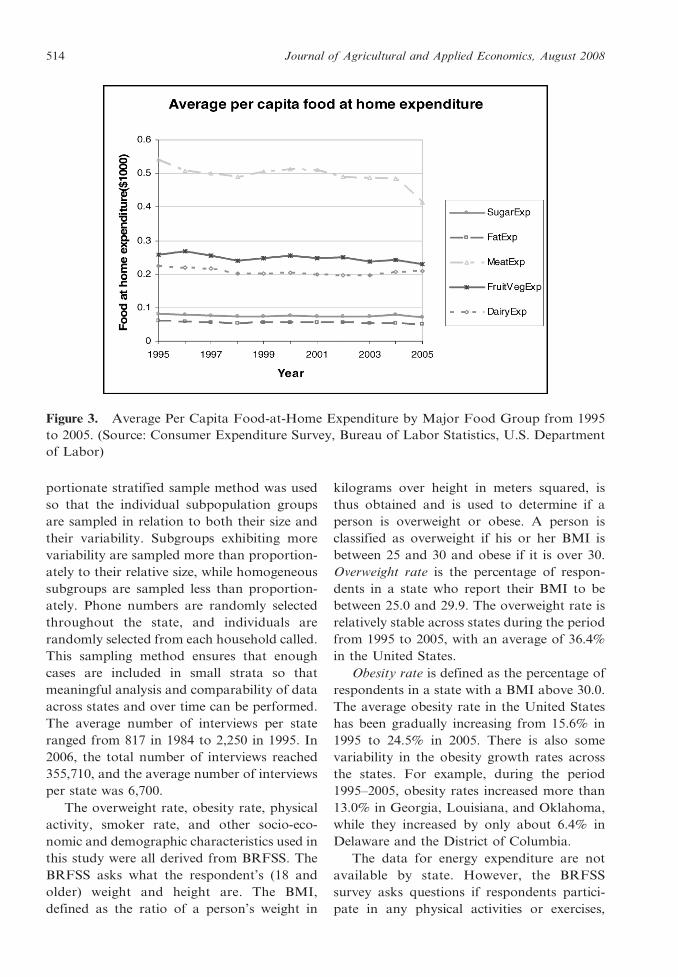
In general, fats, sugars, cereals, potatoes,

and meat products are high-energy-dense

foods, relative to vegetables, fruits, and whole

grains, which contain less energy. Despite the

rising obesity rate, Figures 2 and 3 shows that

the real per capita expenditure on fat, sugar,

and meat at home is stable and as such rules out

the possibility of the link between rising obesity

with the consumption of energy-dense food.

However, factors such as growing consumption

of snacks, fast foods, and soft drinks from food

away from home may be the significant drivers

that influence obesity rates. To accommodate

these important considerations, we collected

data for food expenditure at home and away

from home from the Consumer Expenditure

Survey of the BLS. These expenditures were

then deflated using their corresponding CPIs.

However, the data are available only by region;

thus, the numbers assigned to states within that

region have the same value. The average real

per capita personal income is approximately

$16,500, and approximately $3,060 is spent on

food and $1,800 allotted for food-at-home

expenditures. About $1,260 is spent for food

away from home.

Although national estimates of obesity

trends among U.S. adult populations have

been periodically obtained through surveys

conducted by the National Center for Health

Statistics, these data are not available on a

state-specific basis. This deficiency is viewed as


Table 1. Descriptive Statistics

Variable Definition

Mean and Standard

Deviation

RPincome Real per capita personal income, $1,000 16.150 (2.647)

FoodExp Real per capita food expenditure, $1,000 3.060 (0.202)

FoodhomeExp Real per capita food expenditure at home, $1,000 1.795 (0.127)

FoodawayExp Real per capita food expenditure away from home, $1,000 1.257 (0.111)

Obesity Percentage of adult respondents in a state whose BMI is between

25.0 and 29.9

0.199 (0.038)

Overweight Percentage of adult respondents in a state whose BMI is above

30.0

0.364 (0.016)

Combined 5 obesity + overweight 0.563 (0.044)

Lobesity 5 log(obesity/(1 2 obesity)) 21.411 (0.245)

Loverweight 5 log(overweight/(1 2 overweight)) 20.557 (0.071)

LCombined 5 log(combined/(1 2 combined)) 0.257 (0.178)

Noex Percentage of adult respondents in a state who report no leisure-

time physical activity during the past month

0.262 (0.059)

Smoke Percentage of adult respondents in a state who have ever smoked

100 cigarettes in their lifetime and reported smoking every day

or some days

0.228 (0.031)

Education

LessHigh Percentage of adult respondents who did not complete high

school in a state

0.119 (0.039)

High Percentage of adult respondents who completed high school in a

state

0.324 (0.042)

PostHigh Percentage of adult respondents who completed grade 12 or GED

in a state

0.275 (0.035)

College Percentage of adult respondents who completed college or above

in a state

0.281 (0.057)

Race

White Percentage of white adult respondents in a state 0.787 (0.151)

Black Percentage of black adult respondents in a state 0.087 (0.104)

Hispanic Percentage of Hispanic adult respondents in a state 0.070 (0.081)

Other Percentage of adult respondents who are not white, black, or

Hispanic in a state

0.048 (0.075)

Age

Age18_24 Percentage of adult respondents whose age is between 18 and 24

in a state

0.129 (0.013)


in a state

0.187 (0.019)


in a state

0.209 (0.015)


in a state

0.180 (0.015)


in a state

0.121 (0.011)

Age65 Percentage of adult respondents whose age is 65 or above in a

state

0.173 (0.024)

Gender

Female Percentage of female adult respondents in a state 0.517 (0.010)

Male Percentage of male adult respondents in a state 0.483 (0.010)


critical for state health agencies whose prima-

ry role is mobilizing resources to reduce rising

trends in obesity and their consequent illness-

es. The Center for Disease Control and

Prevention (CDC) established the BRFSS to

track health conditions and risk behaviors,

including obesity, among adults in the United

States. The BRFSS is the world’s largest

ongoing telephone health survey system,

consisting of annual telephone surveys of

persons 18 and older and conducted by state

health departments in collaboration with the

CDC. It collects data on actual behaviors

rather than on attitudes or knowledge that

would be especially useful for planning,

initiating, supporting, and evaluating health

promotion programs at the state level. Each

year, the CDC publishes an annual report,

‘‘Health Risks in the United States Behavioral

Risk Factor Surveillance System at a Glance.’’

Therefore, BRFSS annual data from 1995 to

2005, rather than the NHANES data, are used

in our study.

The CDC developed a standard question-

naire for states to use to provide data that

could be compared across states. The dispro-

Variable Definition

Mean and Standard

Deviation

Region

Midwest Dichotomous variable that equals 1 if the state lies in Midwest, 0

otherwise

0.235 (0.425)

South Dichotomous variable that equals 1 if the state lies in South, 0

otherwise

0.333 (0.472)

Northeast Dichotomous variable that equals 1 if the state lies in Northeast,

0 otherwise

0.176 (0.382)

West Dichotomous variable that equals 1 if the state lies in West, 0

otherwise

0.255 (0.436)

Note: Standard errors are in parentheses. Sample size is 561 including 50 states and Washington, D.C., from 1995 to 2005.

Table 1. Continued.

Figure 2. Average Per Capita Food Expenditure at Home and Away from Home from 1995 to

2005. (Source: Consumer Expenditure Survey, Bureau of Labor Statistics, U.S. Department

of Labor)


portionate stratified sample method was used

so that the individual subpopulation groups

are sampled in relation to both their size and

their variability. Subgroups exhibiting more

variability are sampled more than proportion-

ately to their relative size, while homogeneous

subgroups are sampled less than proportion-

ately. Phone numbers are randomly selected

throughout the state, and individuals are

randomly selected from each household called.

This sampling method ensures that enough

cases are included in small strata so that

meaningful analysis and comparability of data

across states and over time can be performed.

The average number of interviews per state

ranged from 817 in 1984 to 2,250 in 1995. In

2006, the total number of interviews reached

355,710, and the average number of interviews

per state was 6,700.

The overweight rate, obesity rate, physical

activity, smoker rate, and other socio-eco-

nomic and demographic characteristics used in

this study were all derived from BRFSS. The

BRFSS asks what the respondent’s (18 and

older) weight and height are. The BMI,

defined as the ratio of a person’s weight in

kilograms over height in meters squared, is

thus obtained and is used to determine if a

person is overweight or obese. A person is

classified as overweight if his or her BMI is

between 25 and 30 and obese if it is over 30.

Overweight rate is the percentage of respon-

dents in a state who report their BMI to be

between 25.0 and 29.9. The overweight rate is

relatively stable across states during the period

from 1995 to 2005, with an average of 36.4%

in the United States.

Obesity rate is defined as the percentage of

respondents in a state with a BMI above 30.0.

The average obesity rate in the United States

has been gradually increasing from 15.6% in

1995 to 24.5% in 2005. There is also some

variability in the obesity growth rates across

the states. For example, during the period

1995–2005, obesity rates increased more than

13.0% in Georgia, Louisiana, and Oklahoma,

while they increased by only about 6.4% in

Delaware and the District of Columbia.

The data for energy expenditure are not

available by state. However, the BRFSS

survey asks questions if respondents partici-

pate in any physical activities or exercises,

Figure 3. Average Per Capita Food-at-Home Expenditure by Major Food Group from 1995

to 2005. (Source: Consumer Expenditure Survey, Bureau of Labor Statistics, U.S. Department

of Labor)


such as running, calisthenics, golf, gardening,

or walking, other than regular job during the

past month, which would be used to proxy the

energy expenditure variable. Thus, NOEX

represents the percentage of respondents in

the state who report no leisure-time physical

activity during the past month. On average,

26.2% of adults have no leisure-time physical

activity during the past month. During the 11-

year period, the no-leisure-time physical ac-

tivity rate has fluctuated around 21.1% to

51.2% in Arizona, while in Texas it has been

relatively stable at 27.8%.

In 1990, the U.S. Surgeon General’s Office

determined that between 58% and 87% of

those individuals who quit smoking gained

weight and that, on average, those who quit

gained four pounds more than those who

continued to smoke. While these findings seem

to indicate short-run weight gains, there is

little evidence to show a direct link between

smoking and steady state weight. Chou,

Grossman, and Saffer reported that higher

cigarette prices leads to increased body weight.

Using cigarette tax rather than the cigarette

price and controlling for nonlinear time

effects, Gruber and Frakes found negative

effects of cigarette taxes on body weight,

implying that reduced smoking leads to lower

body weight. This finding also motivated the

study to examine the smoking effects on

obesity. The BRFSS survey reports the

percentage of respondents in a state who have

smoked 100 cigarettes in their lifetime and

who smoke every day or some days (smoke).

These data were also obtained from the

BRFSS, and, on average, 22.2% of the sample

are smokers.

The four education variables are represent-

ed by the percentage of respondents in a state

who have less than a high school education

(LessHigh), who have a high school education

(High), who have a general equivalency

diploma (GED) or who completed 12th grade

(PostHigh), and who completed college or

higher (College). On average, about 12% of

the sample have less than high school educa-

tion, 32% of the sample completed high

school, 28% received a GED or completed

12th grade, and 28% have a college degree.

Ethnicity is divided into four groups: white

(White), black (Black), Hispanic (Hispanic),

and others (Other). The numbers reflect the

percentage of each race group in a state. Age is

classified into five groups: 18–24, 25–34, 35–

44, 45–54, 55–64, and over 65. Gender was

included with the variable Male being the

base. This denotes the percentage of male and

female population in the state, respectively.

Regional indicator variables, such as Midwest,

South, Northeast, and West, were also includ-

ed with the West variable serving as base.

Empirical Model

In this paper, a panel model with random

effects was used. The general model notation

for panel data format at the state level with

variations in state i at time t is as follows:

ð8ÞYit ~ bXit z ci z uit,

where : i ~ 1, . . . ::N,t ~ 1, . . . . . . ,T

ð9Þ cov Xit,uitð Þ~ 0,

ð10Þ cov Xit,cið Þ~ 0:

Assuming a general linear model for a panel

data, Yit and Xit are the response variable and

its respective covariates indexed at state i at

time period t. The variable ci is the unobserved

individual effect, which is a source of time-

invariant heterogeneity, and uit is an i.i.d

random error term with zero mean and finite

variance. In this model, strong exogeneity is

assumed where the error term uit is uncorre-

lated with the past, present, and future values

of Xit (Equation [9]). Finally, the model

assumes that the vector of regressors Xit is

uncorrelated with the unobservable individual

effects ci (Equation [10]) such that random

effects model is valid. The identification of the

random effects model is obtained through

taking the expectation of Equation (8) (Cam-

eron and Trivedi; Wooldridge), thus obtaining

the conditional expectation:

ð11Þ E YitjXit½ �~ E cijXit½ �z bXit z E mitjXit½ �:

Three dependent variables were used, and

these are state-level obesity rates, overweight


rates, and the combined rate (sum of obesity

and overweight rates). The empirical model is

as follows:

ð12Þ

obesityit=overweightit=combinedit

~ b0 z b1FoodhomExpit

z b2FoodawayExpit

z b3Rpincomeit z b4Noexit

z b5Smokeitz b6Femaleit

z b7Whiteit z b8Blackit

z b9Hispanicitz b10Age18 24it

z b11Age25 34it z b12Age35 44it

z b13Age45 54it z b14Age55 64it

z b15Lesshighitz b16Highit

z b17Collegeit z b18Midwestit

z b19Southit z b20Northeastit

z ci z uit,

where obesity/overweight/combined rates are

the three dependent variables and the explan-

atory factors include state-level expenditures

on food at home and food away from home,

real personal income, percentage of individu-

als who do not exercise, percentage of

individuals who smoke, and gender, ethnicity,

age, education, and region variables.

Since our dependent variables are mea-

sured in percentage terms, we used the log

odds ratio; logP/(1 2 P), where P is the

overweight, obesity, or combined rate in our

estimation. The proposed model was estimat-

ed by the generalized least squares estimator.

We then calculated the marginal effects of the

variables based on the estimated coefficients.

Several hypotheses were put forth in terms

of the relevant drivers of obesity and over-

weight rates. First, food-away-from-home

expenditures are hypothesized to be positively

related to obesity rates, but food-at-home

expenditures are negatively related to obesity

rates. As for ethnicity, recent evidence shows

that obesity is more prevalent among African

Americans and Hispanics than among Whites

and Asian Americans. Hence, we expect the

variables representing the percentage of Afri-

can Americans and the percentage of Hispan-

ics to be positively related to obesity rates. The

no exercise variable (Noex) is expected to also

positively influence obesity rates. Since smok-

ing usually inhibits overeating, we hypothesize

the smoking variable to be negatively related

to obesity rates. We also expect age to be

positively related to obesity rates and educa-

tion to be negatively related to obesity rates.

As for the regions, recent studies point out

that southern states have higher obesity

incidence relative to other states.

Results

Table 2 presents the results obtained from

the panel model with random effects estima-

tion. As discussed previously, we estimated

models for overweight rate, obesity rate, and

combined rate, respectively. The estimates

from these models are separately discussed

next.

Overweight

As shown in Table 2, the per capita food-at-

home expenditures, per capita food-away-

from-home expenditures, per capita personal

income, and percentage of no-leisure-time

physical activity have positive but insignificant

effects (5% significance level) on overweight

rates. However, the percentage of smokers

(Smoke) carries a significant negative coeffi-

cient, suggesting that percentage of smokers

negatively affects state-level overweight rates.

Specifically, a 1% increase in percentage of

smokers decreases overweight rate by 0.127%.

As for education, the percentage of adult

population who completed high school (High)

and the percentage of adult respondents who

completed college and above (College) have

negative effects on overweight rates. This

result is consistent with the findings of Chou,

Grossman, and Saffer.

As for the ethnic factors, the percentage of

Hispanic population has positive effect on

overweight rates, with overweight rate increas-

ing by 0.47% for every 1% increase in

percentage of adult Hispanics in a state. Age

variables are insignificant except for the

positive effect of percentage of adult respon-

dents whose age is between 45 to 54 years old


in a state. The regional factors indicate that

the Midwest, Northeast, and South regions

have higher overweight rates than the West

region. In summary, our results suggest that

the significant factors that positively affect

overweight rates are percentage of respon-

dents who are Hispanic (Hispanic) and per-

centage of respondents in the 45- and 54-year-

old age-group (Age45_54). On the other hand,

variables such as Smoke, high school complet-

ed (High), and College yield negative and

significant effects, while food expenditure at

home (FoodhomeExp) and away from home

(FoodawayExp) do not significantly influence

the overweight rates.

Obesity

Our results indicate that the real per capita

food-at-home expenditures have a negative

effect on obesity rates, while real per capita

food-away-from-home expenditures have a

positive effect on obesity rates. The marginal

effects imply that a $1,000 increase in the per

capita expenditure of food prepared at home

(Foodhomeexp) will translate to a 0.045%

decline in obesity rates, whereas a $1,000

increase in per capita expenditures on food

prepared away from home (Foodawayexp)

will result in a 0.053% increase in obesity rates.

The results also suggest declining positive

marginal effects on obesity rates as education

level increases. As for ethnicity, we find that

percentages of whites, blacks, and Hispanics

have positive effects on obesity rates, but the

marginal effects are higher for blacks than

whites and higher for Hispanics than blacks

and whites. For age, we find age groupings

45–54 (Age45_54) and 55–64 (Age55_64) to be

positively related to obesity rates. The results

suggest that a 1% increase in percentage of

individuals under these age-groups will in-

crease obesity rates by 0.746% and 0.853%,

respectively. Our results also indicate that

percentage of females is negatively related to

obesity rates. For every 1% increase in

females, obesity rate declines by 1.40%.

Finally, all the regional variables are statisti-

cally significant with the South having higher

obesity rate than other regions.

Combined Rate

The combined rate is the sum of the

overweight and obesity rates. The results show

that food-away-from-home expenditures

(Foodawayexp) have a positive effect on the

combined rate, while the reverse is true for

food-at-home expenditures (Foodhomeexp).

The results are consistent with the obesity

category, where in this case a $1,000 increase

in per capita expenditures on food prepared at

home will decrease the combined rate by

0.041%, while an increase of $1,000 in food-

away-from-home expenditures will increase

the combined rate by 0.051%.

The percentage of individuals who com-

pleted at least a college degree is negatively

related to the combined rate. In contrast,

percentages of individuals who are blacks and

Hispanics are positively related to combined

rate. For every 1% increase in number of

blacks and Hispanics, there is 0.06% and

0.15% increase in percentage of overweight

and obese individuals, respectively. Hence, the

percentage of Hispanics has a slightly greater

effect than percentage of blacks on the

combined rate.

In terms of age, the percentages in the

18–24 age-group and 45–65 age-groups

(Age45_54 & Age55_64) are positively related

to the combined rate. The percentage of

females (Female) is negatively related to the

combined rate. All the regional variables are

significant, suggesting higher combined rates

than that of West region, with the South

having the highest marginal effect. This result

is consistent with the findings of the CDC that

indicated higher obesity rates in the South

relative to other parts in the country.

Concluding Remarks

Recent evidence has shown that obesity

among adults has risen significantly in the

United States during the past 20 years. This

paper uses a panel model with random effects

to examine the factors that may influence

state-level obesity and overweight rates in the

United States. Using state-level data from the

1995–2005 BRFSS, our study investigated the


Table

2.

Ran

do

mE

ffec

tsM

od

el

Lo

ver

wei

gh

tL

ob

esit

yL

Co

mb

ined

Co

effi

cien

tM

arg

inal

Eff

ect

Co

effi

cien

tM

arg

inal

Eff

ect

Co

effi

cien

tM

arg

inal

Eff

ect

Inte

rcep

t2

0.3

00

(20.5

6)

0.7

29

(0.7

)0.1

16

1.8

19*

(2.3

4)

Rp

inco

me

0.0

06

(1.8

7)

0.0

01

20.0

02

(20.4

)2

0.0

00

0.0

01

(0.2

2)

0.0

00

Fo

od

ho

mee

xp

0.0

11

(0.2

2)

0.0

02

20.2

83*

(23.7

2)

20.0

45

20.1

66*

(23.0

0)

20.0

41

Fo

od

aw

ayex

p0.0

26

(0.6

6)

0.0

06

0.3

29*

(5.2

6)

0.0

53

0.2

05*

(4.5

)0.0

51

No

ex0.0

43

(0.5

4)

0.0

10

20.6

94*

(25.2

3)

20.1

11

20.4

05*

(24.1

8)

20.1

00

Sm

ok

e2

0.5

47*

(23.4

4)

20.1

27

0.3

51

(1.2

7)

0.0

56

20.3

43

(21.6

9)

20.0

84

Ed

uca

tio

n

Les

shig

h2

0.2

63

(21.4

8)

20.0

61

1.2

01*

(3.9

8)

0.1

91

0.1

47

(0.6

6)

0.0

36

Hig

h2

0.4

28*

(22.6

1)

20.0

99

0.9

21*

(3.3

2)

0.1

47

0.1

85

(0.9

1)

0.0

45

Co

lleg

e2

0.8

66*

(25.1

7)

20.2

00

0.7

33*

(2.6

4)

0.1

17

20.4

15*

(22.0

4)

20.1

02

Race W

hit

e0.0

56

(1.0

4)

0.0

13

0.2

42*

(2.2

1)

0.0

39

0.1

05

(1.2

8)

0.0

26

Bla

ck2

0.0

47

(20.5

6)

20.0

11

0.6

05*

(4.0

0)

0.0

96

0.2

48*

(2.2

1)

0.0

61

His

pan

ic0.2

04*

(2.2

8)

0.0

47

0.6

62*

(3.6

5)

0.1

06

0.6

16*

(4.5

)0.1

52

Age A

ge1

8_24

0.1

97

(0.5

1)

0.0

46

2.8

42*

(4.0

3)

0.4

53

2.1

47*

(4.0

9)

0.5

28

Age2

5_34

20.6

18

(21.6

5)

20.1

43

20.5

70

(20.8

6)

20.0

91

20.4

30

(20.8

7)

20.1

06

Age3

5_44

0.6

72

(1.7

8)

0.1

56

21.1

15

(21.6

8)

20.1

78

20.1

25

(20.2

6)

20.0

31

Age4

5_54

1.2

07*

(2.7

1)

0.2

79

4.6

80*

(5.9

4)

0.7

46

4.0

55*

(6.9

5)

0.9

98

Age5

5_64

0.1

36

(0.2

5)

0.0

31

5.3

53*

(5.9

9)

0.8

53

4.1

77*

(6.3

7)

1.0

28

Gen

der

Fem

ale

20.5

08

(20.6

5)

20.1

18

28.7

92*

(25.9

)2

1.4

01

25.8

97*

(25.3

)2

1.4

51

Reg

ion

Mid

wes

t0.0

83*

(4.0

2)

0.0

19

0.2

72*

(6.4

4)

0.0

43

0.2

66*

(8.2

9)

0.0

66

So

uth

0.0

73*

(2.9

)0.0

17

0.3

08*

(6.2

6)

0.0

49

0.2

88*

(7.7

6)

0.0

71

No

rth

east

0.0

51*

(2.3

7)

0.0

12

0.1

16*

(2.5

2)

0.0

19

0.1

48*

(4.2

1)

0.0

36


Lo

ver

wei

gh

tL

ob

esit

yL

Co

mb

ined

Co

effi

cien

tM

arg

inal

Eff

ect

Co

effi

cien

tM

arg

inal

Eff

ect

Co

effi

cien

tM

arg

inal

Eff

ect

su

0.0

27

0.0

68

0.0

53

se

0.0

52

0.0

78

0.0

57

R0.2

14

0.4

31

0.4

68

R2:

wit

hin

0.1

50.8

44

0.8

38

bet

wee

n0.4

87

0.6

26

0.5

92

over

all

0.2

87

0.7

62

0.7

4

Wald

chi-

squ

are

134

2,6

41

2,5

15

Pro

b.

chi-

squ

are

00

0

No

te:

t-st

ati

stic

sare

inp

are

nth

eses

.*

ind

icate

sst

ati

stic

all

ysi

gn

ific

an

tat

0.0

5le

vel

.

Table

2.

Co

nti

nu

ed.


effects of real food expenditures at home and

away from home on three different weight-

level categories, namely, obesity rates, over-

weight rates, and sum of both obesity and

overweight rates (combined rate). Our results

indicate that food-at-home expenditures are

negatively related to obesity and combined

rates. On the other hand, food-away-from-

home expenditures are positively related to

obesity and combined rates. This implies that

food away from home plays an important role

in increasing overweight and obesity rates.

Our results point out to the importance of

increasing expenditures on food at home and

decreasing expenditures on food away from

home in reducing obesity rates in the United

States. Hence, policymakers may improve the

effectiveness of nutrition and education pro-

grams by emphasizing the importance of

food-at-home preparation and advising indi-

viduals to be more conscious about the

potential effects of eating away from home

on weight.

There are two caveats that need to be

mentioned, however. First, our results are

based on associations and not causal links.

Future studies should develop a robust

identification strategy to establish possible

causal links between food expenditure types

and obesity rates. Second, the magnitudes of

the effects we found, although statistically

significant, are relatively small. Hence,

policies based on our findings will have quite

limited effect on obesity rates, at least in the

short run.

References

Binkley, J.K., J. Eales, and M. Jekanowski. ‘‘The

Relation Between Dietary Change and Rising

US Obesity.’’ International Journal of Obesity

24(2000):1032–39.

Cameron, A.C., and P.K. Trivedi. Microecono-

metrics: Methods and Applications. New York:

Cambridge University Press, 2005.

Centers for Disease Control and Prevention,

Behavioral Risk Factor Surveillance System

Survey Data, Atlanta: U.S. Department of

Health and Human Services, Internet site:

www.cdc.gov/brfss.

Chou, S.Y., M. Grossman, and H. Saffer. ‘‘An

Economic Analysis of Adult Obesity: Results

from the Behavioral Risk Factor Surveillance

System.’’ Journal of Health Economics 23(2004):

565–87.

Cutler, D.M., E.L. Glaeser, and J.M. Shapiro. ‘‘Why

Have Americans Become More Obese?’’ Journal

of Economic Perspectives 17,3(2003):93–118.

Drewnowski, A., and N. Darmon. ‘‘The Economics

of Obesity: Dietary Energy Density and Energy

Cost.’’ American Journal of Clinical Nutrition

82(Suppl. 2005a):265–73.

———. ‘‘Food Choices and Diet Costs: An Econo-

mic Analysis.’’ Journal of Nutrition 135(April

2005b):900–904.

Economic Research Service. ‘‘Table 1: Food and

Alcoholic Beverages: Total Expenditures.’’ Food

CPI, Prices, and Expenditures. Washington,

DC: Economic Research Service, 2003.

———. ‘‘Table 5: Daily Food Consumption at

Different Locations: All Individuals Ages 2 and

Older.’’ Daily Diet and Health: Food Consump-

tion and Nutrient Intake Tables. Washington,

DC: Economic Research Service, 2000.

French, S.A., L. Harnack, and R.W. Jeffery. ‘‘Fast

Food Restaurant Use Among Women in the

Pound of Prevention Study: Dietary, Behavioral

and Demographic Correlates.’’ International

Journal of Obesity 24(2000):1353–59.

Gruber, J., and M. Frakes. ‘‘Does Falling Smoking

Lead to Rising Obesity?’’ Journal of Health

Economics 25,2(March 2006):183–97.

Jeffery, R.W., and S.A. French. ‘‘Epidemic Obesity

in the United States: Are Quick-Service

Foods and Television Viewing Contributing?’’

American Journal of Public Health 88(1998):

277–80.

Kant, A.K. ‘‘Consumption of Energy-Dense, Nu-

trient-Poor Foods by Adult Americans: Nutri-

tional and Health Implications: The Third

National Health and Nutrition Examination

Survey, 1988–1994.’’ American Journal of Clin-

ical Nutrition 72(2000):929–36.

Lakdawalla, D., and T. Philipson. ‘‘The Growth of

Obesity and Technological Change: A Theoret-

ical and Empirical Examination.’’ National

Bureau of Economic Research Working Paper

no. 8946, 2002.

Loureiro, M., and R.M. Nayga. ‘‘International

Dimensions of Obesity and Overweight Related

Problems: An Economics Perspective.’’ Ameri-

can Journal Agricultural Economics 87(2005):

1147–53.

McCrory, M.A., P.J. Fuss, N.P. Hays, A.G. Vinken,

A.S. Greenberg, and S.B. Roberts. ‘‘Overeating

in America: Association Between Restaurant

Food Consumption and Body Fatness in


Healthy Adult Men and Women Ages 19 to 80.’’

Obesity Research 7(1999):564–71.

Nielsen, S.J., R.A.M. Siega, and B.M. Popkin.

‘‘Trends in Energy Intake in U.S. Between 1977

and 1996: Similar Shifts Seen Across Age

Groups.’’ Obesity Research 10(2002):370–78.

Philipson, T. ‘‘The World-Wide Growth in Obesity:

An Economic Research Agenda.’’ Health Eco-

nomics, 2001.

Philipson, T., and R.A. Posner. ‘‘The Long Growth

in Obesity as a Function of Technological

Change.’’ National Bureau of Economic Re-

search Working Paper no. 7423, 1999.

Putnam, J., J. Allshouse, and L.S. Kantor. ‘‘U.S.

Per Capita Food Supply Trends: More Calories,

Refined Carbohydrates and Fats.’’ Food Review

25(2002):2–15.

Rashad, I. ‘‘Structural Estimation of Caloric

Intake, Exercise, Smoking, and Obesity.’’ Quar-

terly Review of Economics and Finance 46(2006):

268–83.

Schofield, W.N., C. Schofield, and W.P.T. James.

‘‘Basal Metabolic Rate—Review and Prediction

Together with Annotated Bibliography of

Source Material.’’ Human Nutrition: Clinical

Nutrition 39C(Suppl. 1, 1985):5–96.

The Surgeon General’s Call to Action to Prevent and

Decrease Overweight and Obesity. Washington,

DC: U.S. Department of Health and Human

Services, 2001.

U.S. Department of Commerce, Bureau of Eco-

nomic Analysis. State Annual Personal Income,

SA1-3. Internet site: www.bea.gov/regional/spi/

default.cfm?satable5summary.

U.S. Department of Labor, Bureau of Labor

Statistics. Consumer Expenditure Survey. Inter-

net site: www.bls.gov/cex.

———. Consumer Price Index—All Urban Con-

sumers, Internet site: www.bls.gov/cpi.

Wooldridge, J. Econometric Analysis of Cross

Section and Panel Data. Cambridge, MA:

MIT Press, 2002.


the effect of food-away-from-home and food-at-home expenditures on

Documents