household food expenditures across income groups: do poor

Conference Paper

Center for International Food and Agricultural Policy

Research, Food and Nutrition, Commodity and Trade,

Development Assistance, Natural Resource and Environmental Policy Household Food Expenditures Across Income Groups: Do Poor

Households Spend Differently than Rich Ones?

by

Amy L. Damon, * Robert P. King* and Ephraim Leibtag** *University of Minnesota; **ERS/USDA

Center for International Food and Agricultural Policy University of Minnesota

Department of Applied Economics 1994 Buford Avenue

St. Paul, MN 55108-6040 U.S.A.

Paper presented at the 10th Joint Conference on Food, Agriculture and the Environment, Duluth, Minnesota, August 27-30, 2006.

Household Food Expenditures across Income Groups: Do Poor Households Spend Differently than Rich Ones?

Amy L. Damon

Department of Applied Economics University of Minnesota

St. Paul, MN 55108

Robert P. King Department of Applied Economics

University of Minnesota St. Paul, MN 55108

Ephraim Leibtag

Food Markets Branch FRED-ERS-USDA Washington, DC

Selected Paper prepared for presentation at the American Agricultural Economics Association Annual Meeting, Long Beach, California, July 23-26, 2006

Abstract: The Life Cycle - Permanent Income Hypotheses (LCPIH) suggests that the timing of an income payment or government transfer should have no effect on the expenditures of the recipient. In this paper we test the LCPIH against a dynamic model of household consumption which predicts clustered food expenditure. We use data from 7,013 households in fifty-two urban and peri-urban markets throughout the United States containing detailed daily expenditure data collected by ACNielsen Homescan for 2003. Specifically, we examine aggregate food expenditure patterns, shopping trip patterns, and expenditure patterns across retail channels over calendar weeks, weekly seven day cycles, and days of the week. Our main finding is that households in the lowest 25 percent of the income distribution that have zero employed people have a significantly higher differenced expenditure level in the beginning of the month and significantly lower differenced expenditure in the last week or weeks of the calendar month, thus rejecting the LCPIH. Further, we find that, in general, households do not use convenience stores as a complementary retail channel to the grocery channel.

Acknowledgements: This research was funded by the Economics Research Service of the United States Department of Agriculture and by the Minnesota Agricultural Experiment Station. Opinions and conclusions in this article are those of the authors and do not necessarily reflect those of USDA or the University of Minnesota. Copyright 2006 by Amy L. Damon, Robert P. King, and Ephraim Leibtag. All rights reserved. Readers may make verbatim copies of this document for non-commercial purposes by any means, provided that this copyright notice appears on all copies.

1

The Life Cycle - Permanent Income Hypotheses (LCPIH) suggests that the timing

of an income payment or government transfer should have no effect on the expenditures

of the recipient. This outcome, however, stands in contrast with anecdotal evidence

indicating that individuals and households cluster their expenditures around the time of

income payments or government assistance distributions. Food expenditures, given their

relative frequency compared to other purchases, are typically noted to be especially

vulnerable to cyclical fluctuations in purchasing patterns. On May 15, 2006 the New

York Times (Associated Press, p. 25) reported that the food expenditure cycle in

Michigan was so pronounced in poorer neighborhoods that food retailers were lobbying

for a change in the way federal assistance programs were distributed in order to even out

the swings in customer traffic, which retailers claim make it difficult to provide sufficient

food stocks and staff.

This article makes two contributions toward further understanding food

expenditure cycles using detailed household food expenditure data for 7,013 households

in fifty-two urban areas throughout the United States. Specifically, we ask: 1) Do

consumers’ expenditure patterns or trips to the store exhibit cyclical, weekly, or daily

patterns? 2) Does consumers’ use of alternative food retail channels for food expenditures

vary cyclically throughout the month?

We examine monthly household food expenditure patterns across five income

groups. Understanding these expenditure patterns across income groups has implications

for both private sector retail interests, such as those highlighted by the recent newspaper

article, as well as policy makers concerned with the nutrition and food security of low

income households. Expenditure patterns over the course of a month are of interest to

2

food retailers, since “bumps” in food expenditures – especially for perishable items such

as dairy, meat, and eggs – have implications for inventory management at the retail level.

Further, cyclical purchasing patterns of vegetables, dairy products, and meat products, in

low income households may imply that these households experience monthly disruptions

in their nutritional balance.

Cyclical patterns in the allocation of food expenditures across market channels are

also of interest. Constraints imposed on low-income households by small cash reserves,

lack of access to private transportation, and limited food storage space in their homes

may make it less attractive to shop in club stores that cater to “stock-up” shoppers.

Further, if it is true that poor shoppers supplement their monthly grocery store trip with

purchases at neighborhood convenience stores and small grocery stores, this implies the

household location influences a low income household’s optimal consumption bundle

given the higher prices paid at these smaller stores.

In the sections that follow, we first review the relevant literature, focusing on

those studies which have upheld and disproved the LCPIH and then those that have

examined the LCPIH specifically with respect to food. Next, we present an alternative to

the LCPIH in the form of a dynamic model of food purchasing patterns that is the basis

for the alternative hypotheses formulation. We then describe the data sources for this

article, describe our empirical estimation strategy, and present results. The article

concludes with a summary discussion and concluding remarks.

Literature Review

The LCPIH suggests that the expenditure patterns should be unaffected by the

receipt of a paycheck or income transfer. Results testing the empirical validity of the

3

LCPIH have been mixed. Hall uses Euler equations to test the LCPIH and finds

supporting evidence using time series data to show that no variable, except for current

consumption, has any power in predicting future consumption. Browning and Collado

find empirical evidence supporting the LCPIH using expenditure and income data from

Spain, which suggests that Spanish households smooth their consumption over the year

independent of income flow.

Contrary to these findings, Zeldes and Jappelli et. al. find that liquidity or credit

constraints do impact low income households’ consumption behavior. Stephens (2003)

reports further contradictory evidence suggesting that both the dollar amount and

probability of expenditures increase directly after the receipt of a social security check.

Shapiro also rejects the LCPIH hypothesis in an analysis of changes in individual

consumption patterns in response to receipt of food stamps. Huffman and Barenstein find

consumption expenditure declines between paychecks in the UK. These studies are a

sample of the numerous studies that exist on both sides of this debate.

A number of studies have examined food consumption (e.g. Stephens, 2003) in

light of the LCPIH. Low income households’ food purchasing and consumption patterns

have received considerable attention in recent literature. There is growing conclusive

evidence that low income households exhibit cyclical food consumption and expenditure

behavior that is dependent on the timing of their paycheck or government transfer. Wilde

and Ranney find that the mean food energy intake for food stamp recipients drops

significantly by the fourth week of the month. Stephens (2003) supports the cyclical

expenditure hypothesis with his work documenting how food expenditures depend on

social security checks, finding that expenditures spike immediately after the receipt of a

social security check. Further advancing the idea that poor households exhibit fluctuating

4

food supplies, Shapiro finds that caloric intake declines 10 to 15 percent over the food

stamp month. Stephens (2002) examines the expenditure patterns of perishable, or

immediately consumed goods using data from the United Kingdom, and finds that

consumption for households that face liquidity constraints is influenced by the timing of

pay-check receipt.

These studies provide evidence that government transfers influence the food

intake and expenditure patterns of recipients. However, they do not offer a clear picture

of food expenditure patterns for the working poor in general. Previous studies suggest

that food stamp recipients cluster their expenditures around the time of the transfer and

typically have one large grocery shopping trip each month as a result of transportation

constraints or lack of storage capacity (Wilde and Ranney). There is anecdotal evidence

that low income households make smaller trips to higher price stores for the rest of the

month.

This article contributes to this body of literature by using a comprehensive data

set documenting all household food expenditure for 7,013 households for each day in

2003 in an empirical analysis based on a simple but robust dynamic programming model

of consumption. We integrate the question of food expenditures into the larger body of

literature testing the LCPIH and examine whether households with different employment

structures in different income groups vary their food expenditure over the course of a

month. We examine this question by testing whether expenditures on food items exhibit

a cyclical pattern and whether the frequency of food shopping trips differs over the

course of a month. We also test whether consumers utilize different food retail channels

over the course of the month.

5

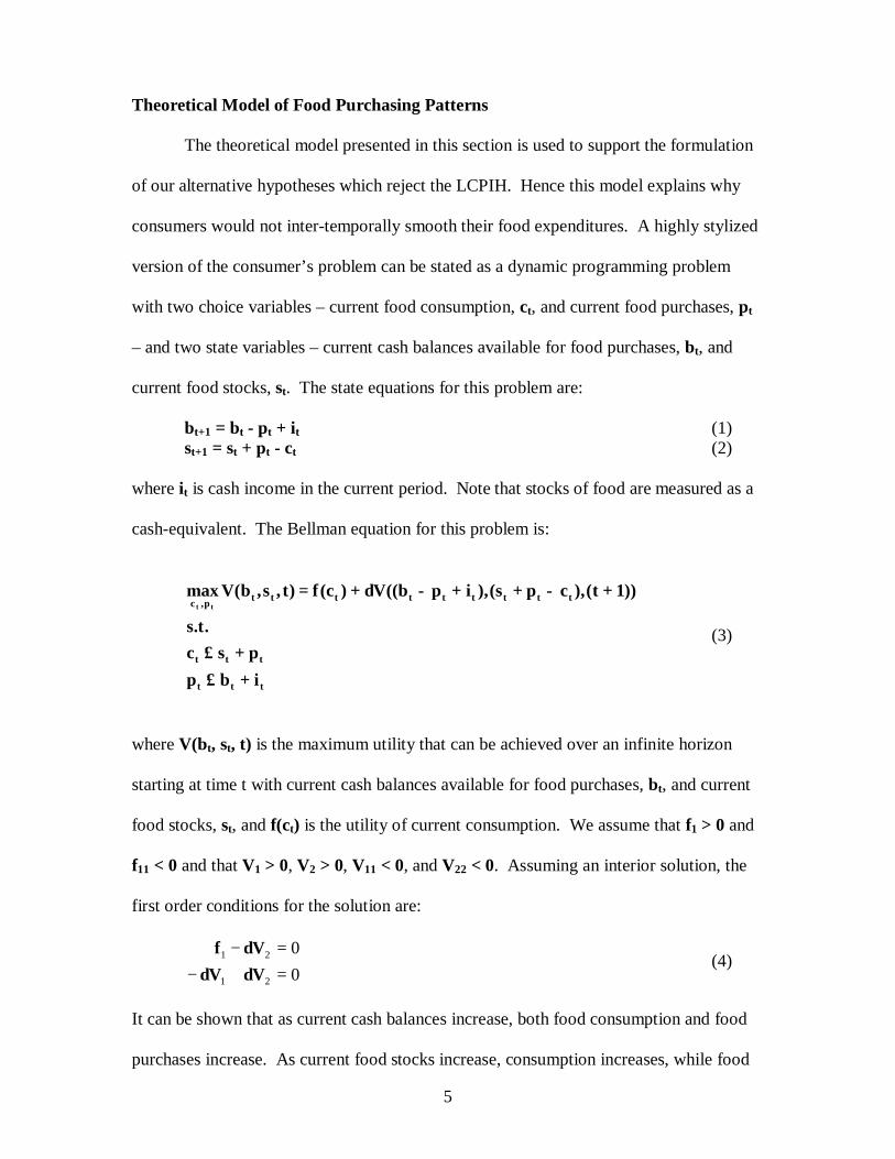
Theoretical Model of Food Purchasing Patterns

The theoretical model presented in this section is used to support the formulation

of our alternative hypotheses which reject the LCPIH. Hence this model explains why

consumers would not inter-temporally smooth their food expenditures. A highly stylized

version of the consumer’s problem can be stated as a dynamic programming problem

with two choice variables – current food consumption, ct, and current food purchases, pt

– and two state variables – current cash balances available for food purchases, bt, and

current food stocks, st. The state equations for this problem are:

bt+1 = bt - pt + it (1) st+1 = st + pt - ct (2) where it is cash income in the current period. Note that stocks of food are measured as a

cash-equivalent. The Bellman equation for this problem is:

ttt

ttt

tttttttttp,c

ibppsc

.t.s

))1t(),cps(),ipb((V)c(f)t,s,b(Vmaxtt

+≤

+≤

+−++−δ+=

(3)

where V(bt, st, t) is the maximum utility that can be achieved over an infinite horizon

starting at time t with current cash balances available for food purchases, bt, and current

food stocks, st, and f(ct) is the utility of current consumption. We assume that f1 > 0 and

f11 < 0 and that V1 > 0, V2 > 0, V11 < 0, and V22 < 0. Assuming an interior solution, the

first order conditions for the solution are:

00

21

21

=+−=−

VVVf

δδδ

(4)

It can be shown that as current cash balances increase, both food consumption and food

purchases increase. As current food stocks increase, consumption increases, while food

6

purchases decrease. Finally, as current income increases, both current consumption and

current food expenditures increase, but the increase is less than the increase in current

income. The magnitude of these effects increases as cash balances and food stocks

approach zero. Together, these results suggest that food purchases for low income

consumers will be concentrated around the time when they receive income or government

transfers and that expenditures for higher income consumers will be less sensitive to

fluctuations in income.

The following null hypothesis is based on the LCPIH:

1. Households will not cluster their food expenditures in a cyclical pattern around pay periods, government transfers of food stamps, or social security checks.

If this hypothesis is rejected, especially for low income households, this result would

provide evidence in support of our alternative model. We also explore two other

hypotheses related to the number of trips and distribution of expenditures among retail

channels:

2. Households will not exhibit cyclical, weekly, or daily patterns in their distribution of expenditures among retail channels.

3. Households will not exhibit different shopping trip cyclical, weekly, or daily

patterns.

Rejection of these null hypotheses would lend support to Stephens’ (2003, 2002) findings

that households do respond to paycheck and government transfers by clustering their food

expenditures around the time of the paycheck or transfer.

Data Sources

We use ACNielsen Homescan data in this article. This unique data set captures

all food expenditures for the participating households, identifying the date and the name

7

of the store where each purchase was made. The sample includes 7,013 households in

fifty-two market areas in the United States for all twelve months of 2003. Market areas

include both urban and peri-urban areas. In addition to food expenditures, the data set

contains demographic information for each household, including variables that measure

household size, household composition, income range, age and education of household

heads, presence of children, and employment status of the household head.

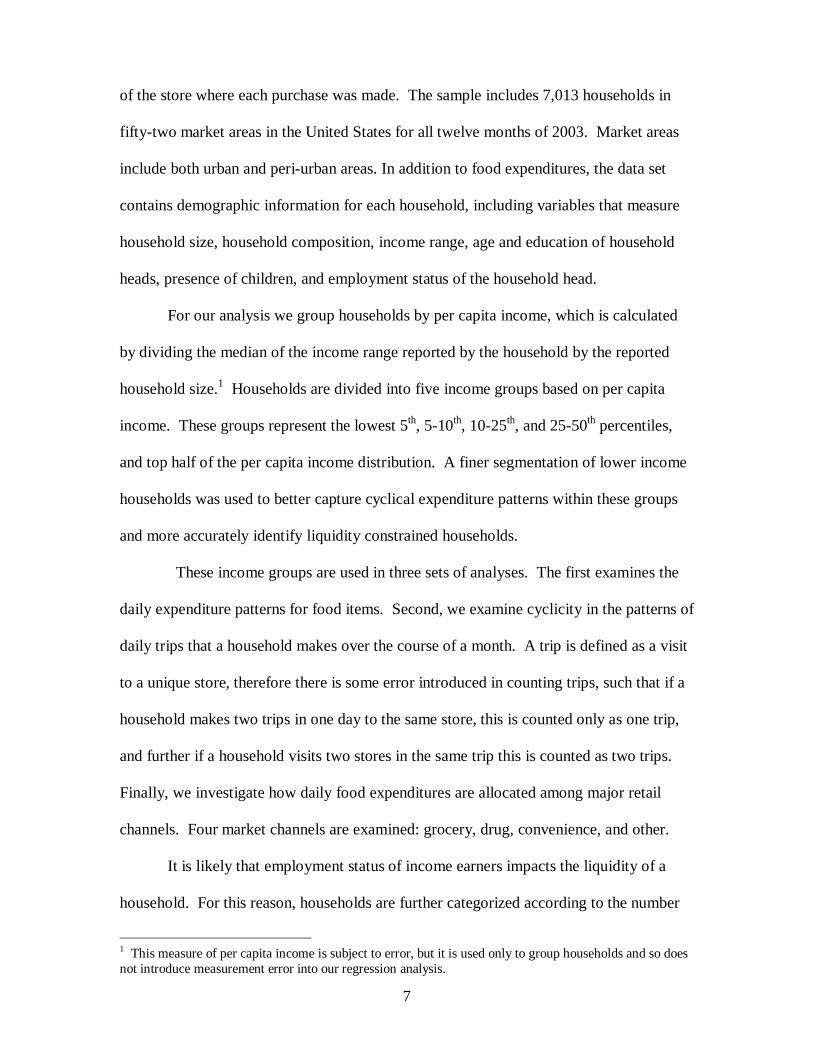
For our analysis we group households by per capita income, which is calculated

by dividing the median of the income range reported by the household by the reported

household size.1 Households are divided into five income groups based on per capita

income. These groups represent the lowest 5th, 5-10th, 10-25th, and 25-50th percentiles,

and top half of the per capita income distribution. A finer segmentation of lower income

households was used to better capture cyclical expenditure patterns within these groups

and more accurately identify liquidity constrained households.

These income groups are used in three sets of analyses. The first examines the

daily expenditure patterns for food items. Second, we examine cyclicity in the patterns of

daily trips that a household makes over the course of a month. A trip is defined as a visit

to a unique store, therefore there is some error introduced in counting trips, such that if a

household makes two trips in one day to the same store, this is counted only as one trip,

and further if a household visits two stores in the same trip this is counted as two trips.

Finally, we investigate how daily food expenditures are allocated among major retail

channels. Four market channels are examined: grocery, drug, convenience, and other.

It is likely that employment status of income earners impacts the liquidity of a

household. For this reason, households are further categorized according to the number

1 This measure of per capita income is subject to error, but it is used only to group households and so does not introduce measurement error into our regression analysis.

8

of employed household heads to examine how employment status is related to

expenditure patterns. Three mutually exclusive and exhaustive employment statuses are

used in the estimation process: i) households with no one employed, including dual

retired household heads (0 employed), ii) households with one income earner, including

single headed households (1 employed), and iii) dual income households (2 employed).

Econometric Model

We consider three cyclical patterns in our analysis. The first is a four week cycle

that captures weekly or bi-weekly pay periods. This twenty-eight day cycle is divided

into four weeks that begin on Mondays. Each week in the cycle is associated with a

binary variable, WEEKCYCLEj, j ∈ {1,2,3,4}, and one and only one of these binary

variables will be equal to one for each day over the course of the year. The second cycle

is the seven days of the week, each of which is associated with a binary variable, DOWk,

k ∈ {1,2,3,4, 5,6,7}. One and only one of these binary variables will be equal to one for

each day over the course of the year. The final cycle in our analysis is the four weeks of

a calendar month, with the first week starting on the first of the month and ending on the

seventh. Because the number of days in a month varies, the fourth “week” of the month

varies in length from seven days in a non-leap year February to nine days in a thirty day

month and ten days in a thirty-one day month. Each of these weeks is associated with a

binary variable, CALWEEKs, s ∈ {1,2,3,4}. Once again, one and only one of these

binary variables will be equal to one for each day over the course of the year.

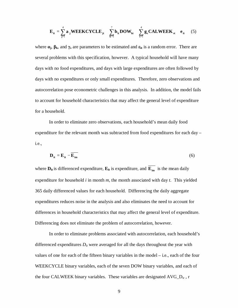
Daily food expenditure for household i on day t, Eit, can be described by the

following expression:

9

∑∑ ∑== =

+++=4

1

4

1

7

1 sitsts

j kktkjtjit CALWEEKDOWWEEKCYCLEE εγβα (5)

where αj, βk, and γs are parameters to be estimated and εit is a random error. There are

several problems with this specification, however. A typical household will have many

days with no food expenditures, and days with large expenditures are often followed by

days with no expenditures or only small expenditures. Therefore, zero observations and

autocorrelation pose econometric challenges in this analysis. In addition, the model fails

to account for household characteristics that may affect the general level of expenditure

for a household.

In order to eliminate zero observations, each household’s mean daily food

expenditure for the relevant month was subtracted from food expenditures for each day –

i.e.,

imitit EED −= (6)

where Dit is differenced expenditure, Eit is expenditure, and imE is the mean daily

expenditure for household i in month m, the month associated with day t. This yielded

365 daily differenced values for each household. Differencing the daily aggregate

expenditures reduces noise in the analysis and also eliminates the need to account for

differences in household characteristics that may affect the general level of expenditure.

Differencing does not eliminate the problem of autocorrelation, however.

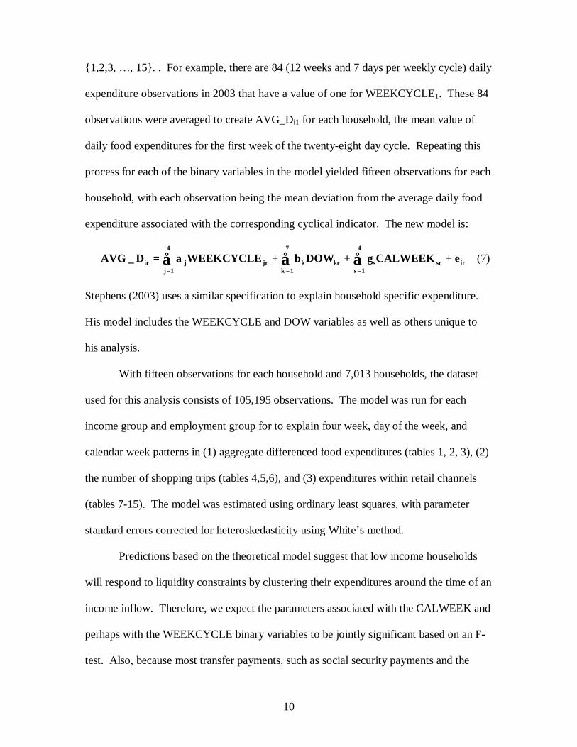
In order to eliminate problems associated with autocorrelation, each household’s

differenced expenditures Dit were averaged for all the days throughout the year with

values of one for each of the fifteen binary variables in the model – i.e., each of the four

WEEKCYCLE binary variables, each of the seven DOW binary variables, and each of

the four CALWEEK binary variables. These variables are designated AVG_Dir , r ∈

10

{1,2,3, …, 15}. . For example, there are 84 (12 weeks and 7 days per weekly cycle) daily

expenditure observations in 2003 that have a value of one for WEEKCYCLE1. These 84

observations were averaged to create AVG_Di1 for each household, the mean value of

daily food expenditures for the first week of the twenty-eight day cycle. Repeating this

process for each of the binary variables in the model yielded fifteen observations for each

household, with each observation being the mean deviation from the average daily food

expenditure associated with the corresponding cyclical indicator. The new model is:

∑∑ ∑== =

ε+γ+β+α=4

1sirsrs

4

1j

7

1kkrkjrjir CALWEEKDOWWEEKCYCLED_AVG (7)

Stephens (2003) uses a similar specification to explain household specific expenditure.

His model includes the WEEKCYCLE and DOW variables as well as others unique to

his analysis.

With fifteen observations for each household and 7,013 households, the dataset

used for this analysis consists of 105,195 observations. The model was run for each

income group and employment group for to explain four week, day of the week, and

calendar week patterns in (1) aggregate differenced food expenditures (tables 1, 2, 3), (2)

the number of shopping trips (tables 4,5,6), and (3) expenditures within retail channels

(tables 7-15). The model was estimated using ordinary least squares, with parameter

standard errors corrected for heteroskedasticity using White’s method.

Predictions based on the theoretical model suggest that low income households

will respond to liquidity constraints by clustering their expenditures around the time of an

income inflow. Therefore, we expect the parameters associated with the CALWEEK and

perhaps with the WEEKCYCLE binary variables to be jointly significant based on an F-

test. Also, because most transfer payments, such as social security payments and the

11

assignment of food stamp benefits are made early in the month, we expect parameters

associated with CALWEEK1 and CALWEEK2 to be statistically significant and positive.

We expect the DOW variables to be jointly significant for all income groups, with the

pattern exhibited by individual parameters reflecting differences in time constraints.

Empirical Results

Food expenditure patterns

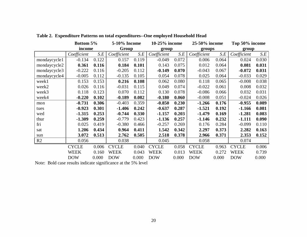
Weekly cycles show little consistent pattern across income groups and

employment structures. If expenditure clustering by weekly cycles were due to liquidity

constraints we would expect to see alternating positive and negative coefficient signs for

those households who get paid every other week, no pattern for those that get paid

weekly, and a single positive week for those that get paid every four weeks,. However,

the dataset used does not have information on paycheck or government transfer

periodicity and therefore it is likely that many different pay period patterns are

represented by the households included. Contrary to prior expectations all three

employment groups exhibit a significant and positive differenced expenditure in the

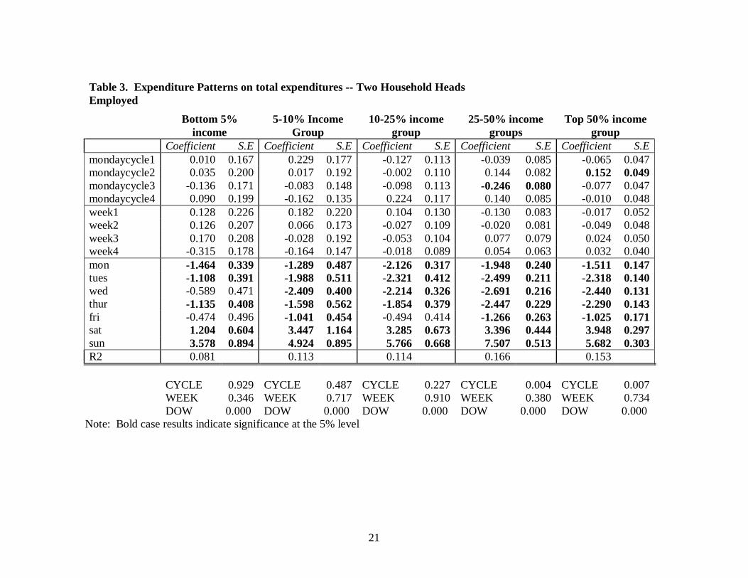
second cycle for the highest income group (tables 1,2 and 3). The third cycle is negative

and significant in the one employed household at the 5% level and negative and

significant at the 10% level in two employed households. It is likely that these cyclical

patterns are not reflective of liquidity constraints resulting from pay period cyclicity, but

rather that they capture the cyclical shopping behavior of higher income households

independent of their pay periods. We likely fail to capture the cyclical nature of low

income households due to liquidity constraints because of the multiplicity of pay periods

represented by the households.

12

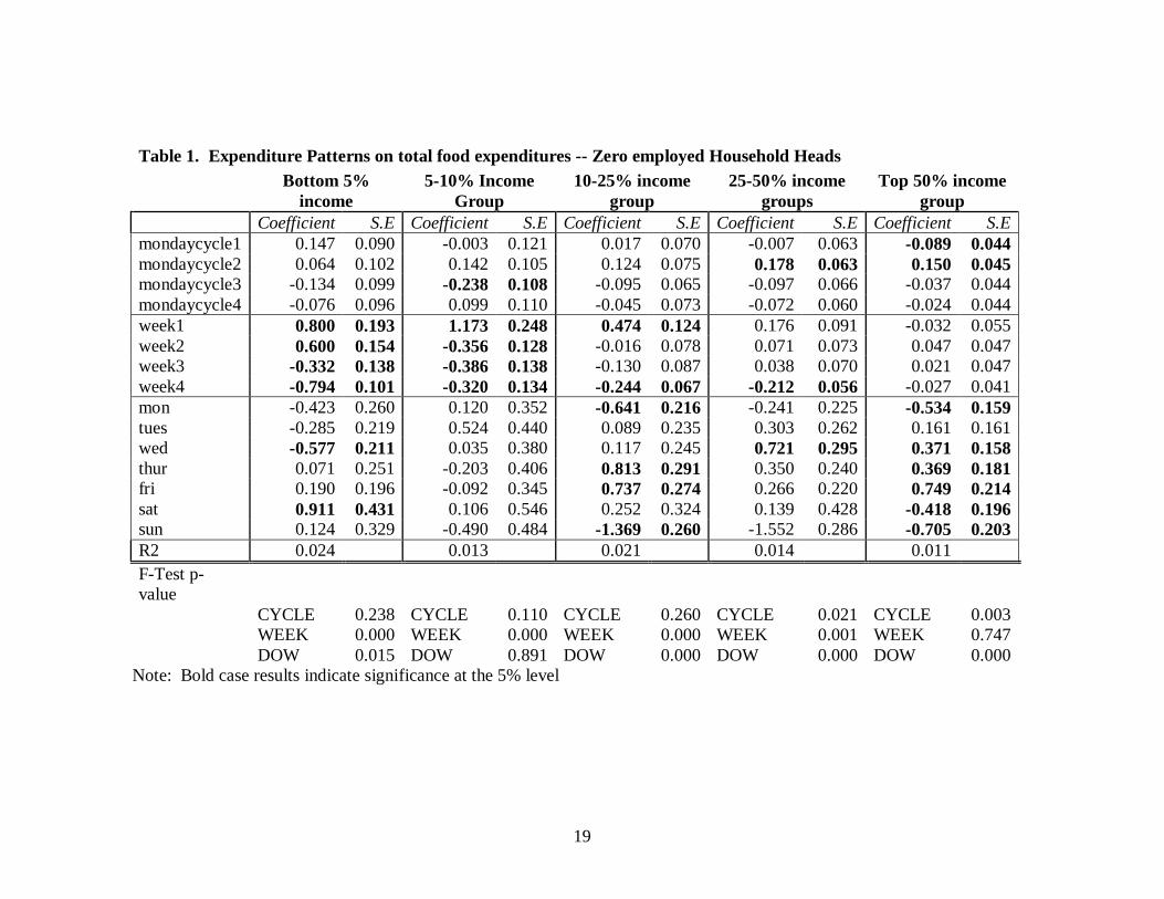
Results concerning week of the calendar month (CALWEEK) show a much more

defined pattern for household food expenditures consistent with our hypothesized

outcomes. Zero employed households are the most likely to depend on some sort of

government transfer, be it social security payments or food stamps, both of which are

issued one time per month and typically at the beginning of the month (table 1). This is

reflected in the lowest three income groups for the zero employed households. The

results suggest that these low income households have positive and significant

differenced expenditures in the first week of the calendar months, with decreasing

expenditures throughout the month and negative and significant expenditures in the last

week of the calendar month. These results offer strong evidence that government

transfers have an important influence on the timing of food expenditures for low income

households.

The weekly pattern in the one employed (table 2) and two employed households

(table 3) is less pronounced. In the one employed households the lowest three income

groups still exhibit negative differenced expenditure in week four of the calendar month,

but the first three weeks, save for week 2 in the 5-10% income group, have positive

differenced expenditures. The two employed households show no calendar week effects

on their food expenditure patterns. This is likely because two income households receive

pay checks several times per month and therefore do not cluster their expenditures around

a single monthly payment.

Day of the week (DOW) effects are highly supportive of our research hypotheses.

In the case of zero employed households (table 1), day of the week effects have a varied

and inconsistent pattern throughout the week. We would expect this result given the low

opportunity cost of time devoted to shopping for these households. The only notable

13

patterns for zero employed households are that the highest income group seems to prefer

to shop midweek and nearly all income groups shop less on Sundays. One and two

employed households (table 2 and table 3) show much stronger results for day of the

week shopping patterns. In both cases, across income groups, households have positive

and statistically significant differenced expenditures for both Saturday and Sunday. This

very likely reflects their increased opportunity cost of shopping during the working week

days.

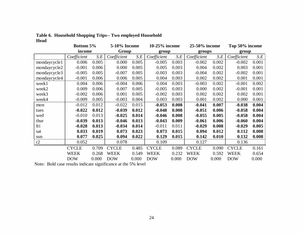
Patterns of food shopping trips

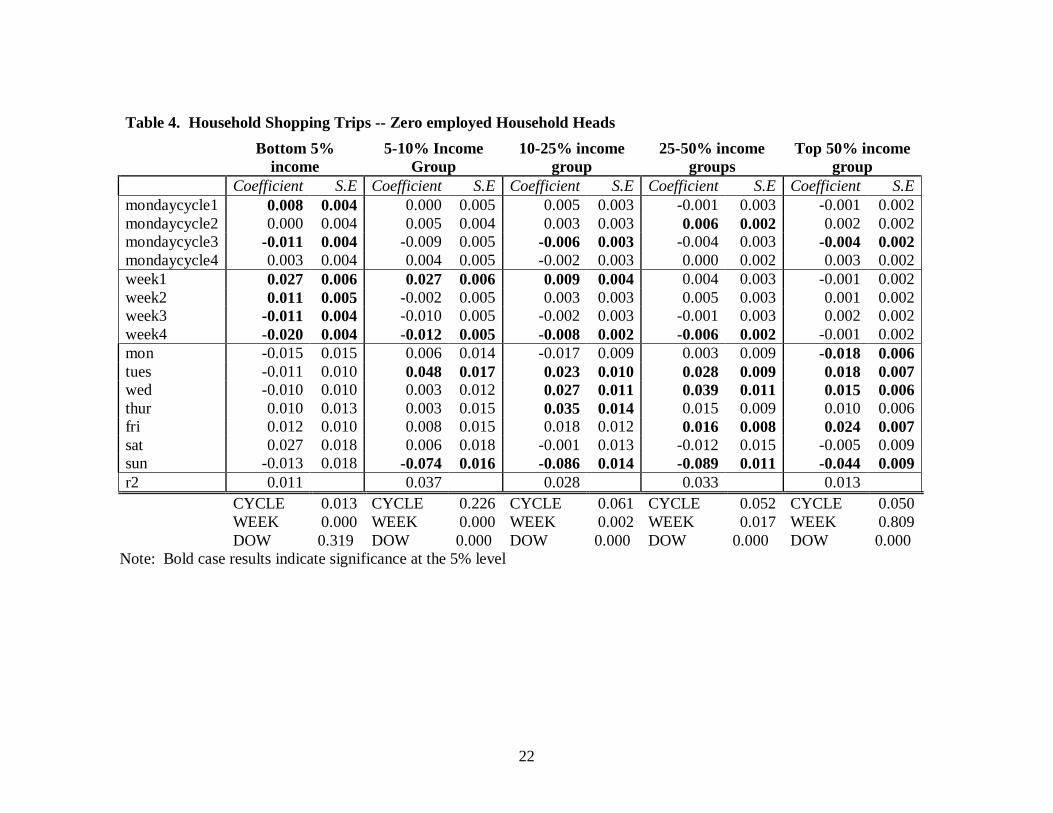
We hypothesize, based on anecdotal evidence that low income households make

one large shopping trip at the beginning of the month and then smaller more frequent

trips toward the end of the month. Our analysis based on the number of daily shopping

trips differenced from the average daily shopping trips for that month does not support

this hypothesis. In the case of zero employed households (table 4) the number of trips a

household makes is largely consistent with food expenditure patterns. The lowest three

income groups make more differenced trips toward the beginning of the calendar month

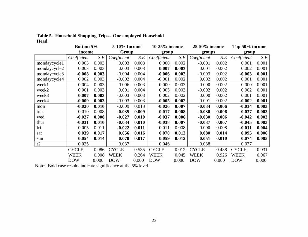
and significantly fewer in the fourth week of the month. One employed households

(table 5) also show some evidence that households make fewer shopping trips in the last

calendar week of the month. Cyclical patterns in both zero and one employed households

show several statistically significant cycle differences, but it is unlikely given their

pattern of trip frequencies that these are due to liquidity constraints. Dual employed

households (table 6) show no cyclical or weekly trip patterns. Day of the week effects

are also consistent with findings from the expenditure analysis. Both one and two

employed households make significantly more trips on Saturday and Sunday, whereas

14

zero employed households make fewer trips on the weekends and significantly fewer on

Sundays.

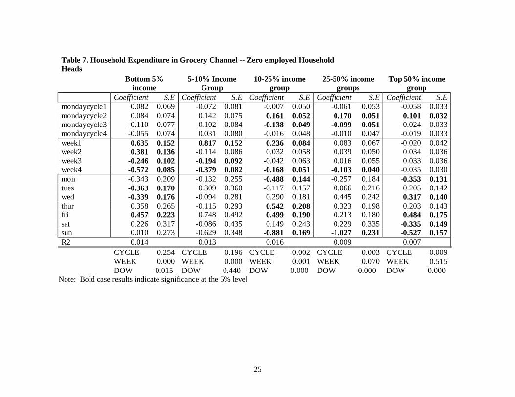
Food expenditure patterns among retail channels

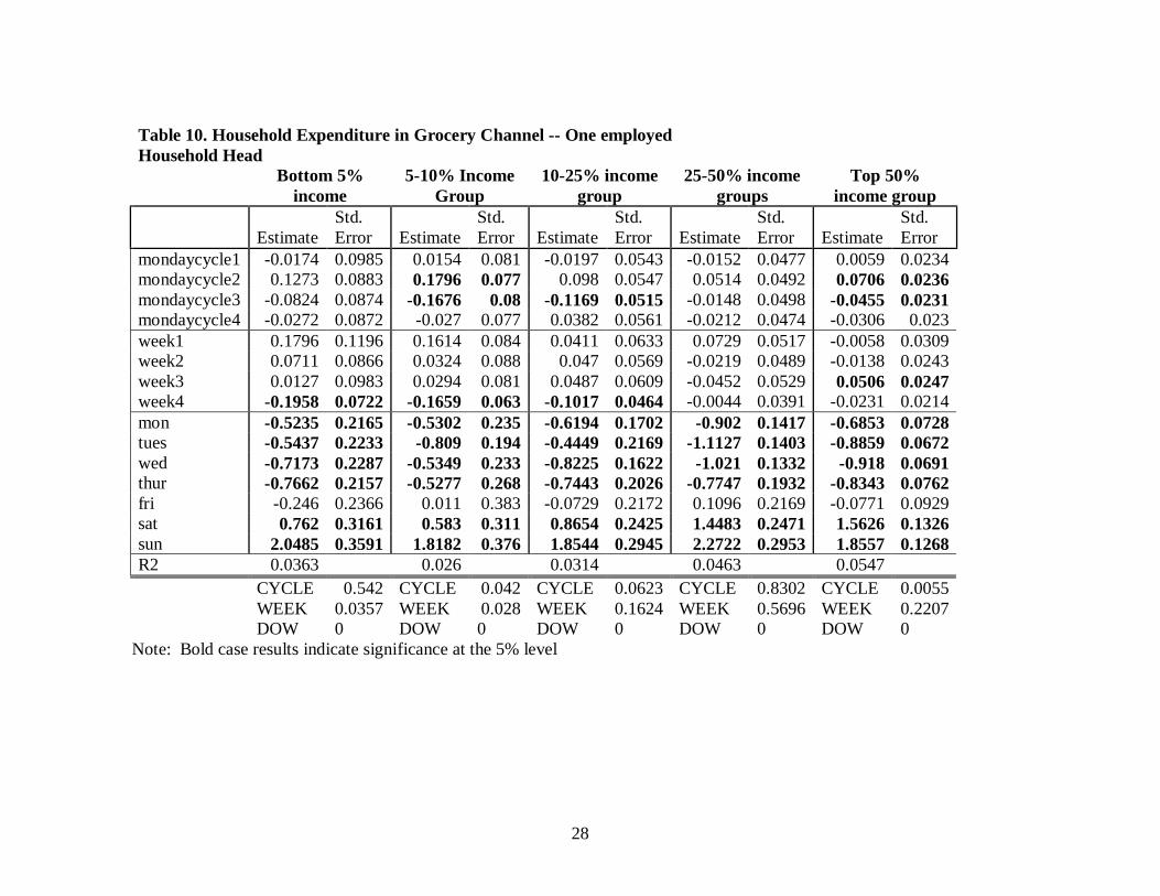
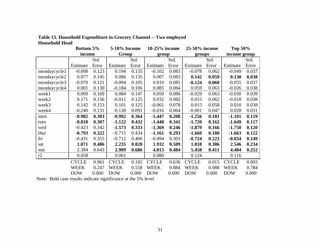
Across income groups and employment groups patterns of expenditures in the

grocery retail channel are similar to patterns that we observed in the aggregate food

expenditure regression analysis (tables 7, 10, and 13). This is reasonable considering that

a majority of household food expenditures are spent in the grocery channel, typically over

70 percent. Lower income households with zero employed spend significantly more in

the beginning calendar months and then expenditures drop off as the month goes on.

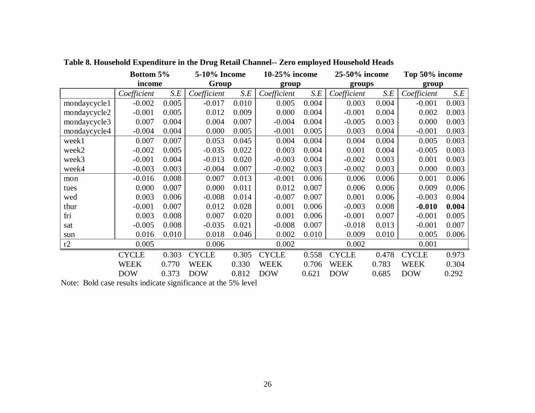
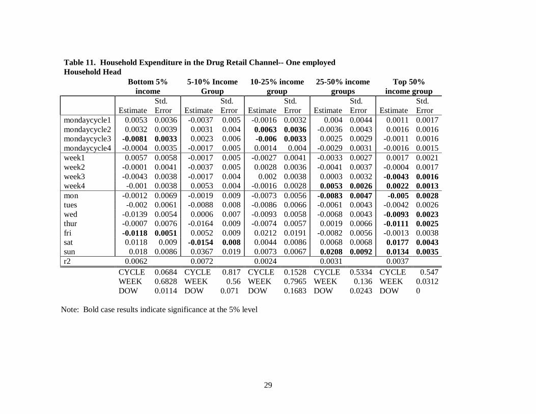
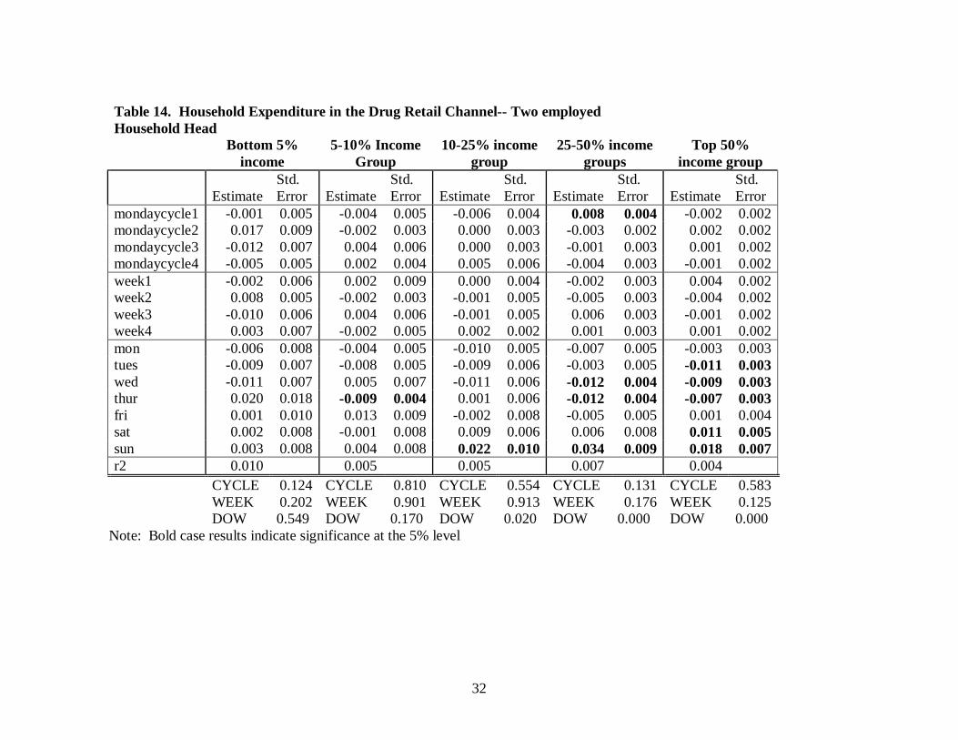
The drug store retail channel shows relatively no significant patterns in the case of

zero employed household (table 8). The signs of coefficient estimates are largely

consistent with those of expenditure patterns in the grocery channel. We fail to reject the

hypothesis that the coefficients are different from zero at any reasonable significance

level in the case of calendar weeks, and we further fail to reject that the coefficients are

different from zero for nearly all of the cycles for all employment groups. Day of the

week expenditure patterns in drug stores are generally consistent with the opportunity

cost induced patterns observed in the aggregate expenditure regressions discussed above.

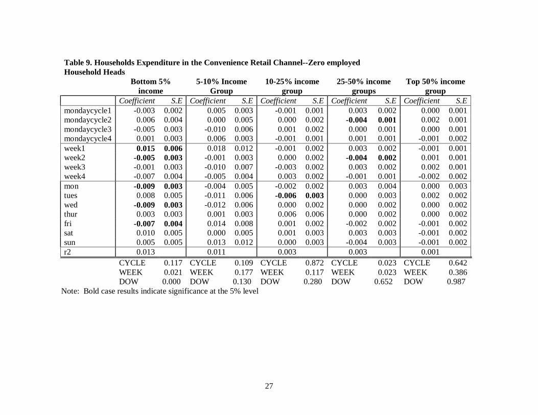
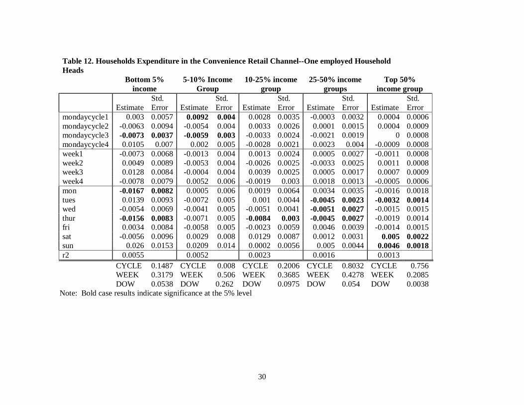
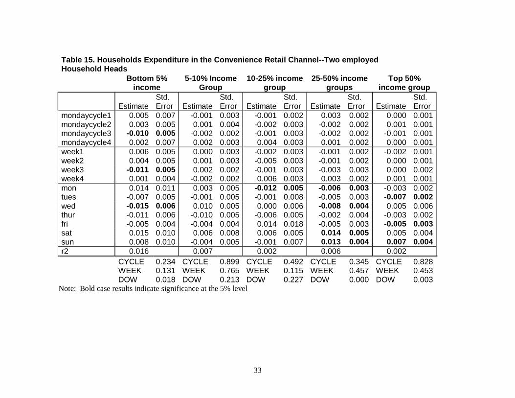
If it is true that low income households make larger trips to the grocery store at

the beginning of the month and smaller trips to smaller retail channels such as

convenience stores toward the end of the month, we would expect to see an increase in

differenced expenditures in convenience stores as the month proceeds. We do not find

evidence of this trend. However, the trend that we do identify may be more troubling in

terms of nutritional balance and household food supply. The lowest 10 percent of the

income distribution for zero employed households exhibits the same spending patterns in

15

each retail food channel, which implies that they are not balancing their food

expenditures toward the end of the month with smaller convenience store trips (table 9),

but rather decreasing their expenditures altogether. This may signal a food insecurity

vulnerability for these households. More generally, across income groups and

employment groups it appears that conveniences store shopping is not a substitute for

grocery store shopping except for possibly in the 10-25 % income group in the zero

employed households (table 9) which has opposite and significant signs associated with

calendar weeks between grocery and convenience store purchases.

Concluding Remarks

This article examines the expenditure patterns of a sample of 7,013 households in fifty-

two urban and peri-urban markets throughout the United States using detailed daily

expenditure data collected by ACNielsen Homescan for 2003. Specifically this article

examines the aggregate food expenditures patterns, shopping trip patterns, and

expenditure patterns within retail channels over calendar weeks, weekly seven day

cycles, and days of the week. Our main findings are that households that have zero

employed people who are in the lowest 25 percent of the income distribution have a

significantly higher differenced expenditure level in the beginning of the month and

significantly lower differenced expenditure in the last week or weeks of the calendar

month. We suggest that this is likely a result of expenditures clustering around

government assistance distributions such as social security payments or food stamps.

Further, we find that the frequency of shopping trips is largely consistent with the pattern

of aggregate expenditures, rejecting the hypothesis that low income households make one

large trip at the beginning of the month and then supplement their household food supply

16

with smaller trips toward the end of the months. Finally, we find that the poorest of the

zero employed households make fewer differenced expenditures in convenience stores

toward the end of the month, suggesting that these households may be vulnerable to food

insecurity in the later parts of the calendar month. These findings are important for policy

makers concerned with the effectiveness of government assistance programs targeted at

reducing household food insecurity. Further, these results support statements by retailers

about monthly spikes in expenditures that make it difficult for them to adequately stock

and staff their retail establishments.

17

References

Associated Press. 2006. “Michigan Grocers Seek Twice-Monthly Food Stamp

Distributions.” New York Times, May 14, pp. 25.

Browning, M. and M.D. Collado. 2001. “The Response of Expenditures to Anticipated

Income Changes: Panel Data Estimates.” American Economic Review 91: 681-

692

Hall, R. 1978. “Stochastic Implications of the Life Cycle-Permanent Income Hypothesis:

Theory and Evidence.” Journal of Political Economy 86: 971-987.

Huffman, D. and M. Barenstein. 2004. "Riches to Rags Every Month? The Fall in

Consumption Expenditures Between Paydays." Discussion Paper IZA No. 1430.

Jappelli, T, J Pischke, N.S. Souleles. 1998. “Testing for Liquidity Constraints in Euler

Equations with Complementary Data Sources.” The Review of Economics and

Statistics. 80:251-262.

Shapiro, J. M. 2005. “Is There a Daily Discount Rate? Evidence from the Food Stamp

Nutrition Cycle.” Journal of Public Economics 89: 303-25.

Stephens Jr., M. 2002. “Paycheck Receipt and the Timing of Consumption.” Working

Paper 9356, NBER.

Stephens Jr., M. 2003. “’3rd of tha Month’: Do Social Security Recipients Smooth

Consumption Between Checks.” American Economic Review 93: 406-22.

Wilde, P.E., and C.K. Ranney. 2000. “The Monthly Food Stamp Cycle: Shopping

Frequency and Food Intake Decisions in an Endogenous Switching Regression

Framework.” American Journal of Agricultural Economics 82: 200-213.

Zeldes, S. 1989 “Consumption and Liquidity Constraints: An Empirical Investigation.”

The Journal of Political Economy. 97: 305-346.

18

APPENDIX 1: REGRESSION RESULTS

19

Table 1. Expenditure Patterns on total food expenditures -- Zero employed Household Heads

Bottom 5%

income 5-10% Income

Group 10-25% income

group 25-50% income

groups Top 50% income

group Coefficient S.E Coefficient S.E Coefficient S.E Coefficient S.E Coefficient S.E

mondaycycle1 0.147 0.090 -0.003 0.121 0.017 0.070 -0.007 0.063 -0.089 0.044 mondaycycle2 0.064 0.102 0.142 0.105 0.124 0.075 0.178 0.063 0.150 0.045 mondaycycle3 -0.134 0.099 -0.238 0.108 -0.095 0.065 -0.097 0.066 -0.037 0.044 mondaycycle4 -0.076 0.096 0.099 0.110 -0.045 0.073 -0.072 0.060 -0.024 0.044 week1 0.800 0.193 1.173 0.248 0.474 0.124 0.176 0.091 -0.032 0.055 week2 0.600 0.154 -0.356 0.128 -0.016 0.078 0.071 0.073 0.047 0.047 week3 -0.332 0.138 -0.386 0.138 -0.130 0.087 0.038 0.070 0.021 0.047 week4 -0.794 0.101 -0.320 0.134 -0.244 0.067 -0.212 0.056 -0.027 0.041 mon -0.423 0.260 0.120 0.352 -0.641 0.216 -0.241 0.225 -0.534 0.159 tues -0.285 0.219 0.524 0.440 0.089 0.235 0.303 0.262 0.161 0.161 wed -0.577 0.211 0.035 0.380 0.117 0.245 0.721 0.295 0.371 0.158 thur 0.071 0.251 -0.203 0.406 0.813 0.291 0.350 0.240 0.369 0.181 fri 0.190 0.196 -0.092 0.345 0.737 0.274 0.266 0.220 0.749 0.214 sat 0.911 0.431 0.106 0.546 0.252 0.324 0.139 0.428 -0.418 0.196 sun 0.124 0.329 -0.490 0.484 -1.369 0.260 -1.552 0.286 -0.705 0.203 R2 0.024 0.013 0.021 0.014 0.011 F-Test p-value CYCLE 0.238 CYCLE 0.110 CYCLE 0.260 CYCLE 0.021 CYCLE 0.003 WEEK 0.000 WEEK 0.000 WEEK 0.000 WEEK 0.001 WEEK 0.747 DOW 0.015 DOW 0.891 DOW 0.000 DOW 0.000 DOW 0.000

Note: Bold case results indicate significance at the 5% level

20

Table 2. Expenditure Patterns on total expenditures--One employed Household Head

Bottom 5%

income 5-10% Income

Group 10-25% income

group 25-50% income


group Coefficient S.E Coefficient S.E Coefficient S.E Coefficient S.E Coefficient S.E mondaycycle1 -0.134 0.122 0.157 0.119 -0.049 0.072 0.006 0.064 0.024 0.030 mondaycycle2 0.361 0.116 0.184 0.101 0.143 0.075 0.012 0.064 0.081 0.031 mondaycycle3 -0.222 0.116 -0.205 0.112 -0.149 0.070 -0.043 0.067 -0.072 0.031 mondaycycle4 -0.005 0.112 -0.135 0.105 0.054 0.078 0.025 0.064 -0.033 0.029 week1 0.153 0.153 0.216 0.108 0.062 0.080 0.118 0.065 -0.008 0.038 week2 0.026 0.116 -0.031 0.115 0.049 0.074 -0.022 0.061 0.008 0.032 week3 0.118 0.123 0.070 0.112 0.130 0.078 -0.086 0.066 0.032 0.031 week4 -0.220 0.102 -0.189 0.082 -0.180 0.060 -0.008 0.051 -0.024 0.026 mon -0.731 0.306 -0.403 0.359 -0.850 0.230 -1.266 0.176 -0.955 0.089 tues -0.923 0.301 -1.406 0.242 -0.637 0.287 -1.521 0.192 -1.166 0.081 wed -1.315 0.253 -0.744 0.330 -1.157 0.203 -1.479 0.169 -1.281 0.083 thur -1.309 0.259 -0.779 0.423 -1.136 0.257 -1.146 0.232 -1.111 0.090 fri 0.025 0.419 -0.380 0.466 -0.257 0.269 0.176 0.284 -0.099 0.110 sat 1.206 0.434 0.964 0.411 1.542 0.342 2.297 0.373 2.282 0.163 sun 3.072 0.513 2.762 0.505 2.518 0.378 2.966 0.371 2.353 0.152 R2 0.056 0.038 0.045 0.058 0.074 CYCLE 0.006 CYCLE 0.040 CYCLE 0.058 CYCLE 0.963 CYCLE 0.006 WEEK 0.160 WEEK 0.043 WEEK 0.013 WEEK 0.272 WEEK 0.739 DOW 0.000 DOW 0.000 DOW 0.000 DOW 0.000 DOW 0.000


21

Table 3. Expenditure Patterns on total expenditures -- Two Household Heads Employed

Bottom 5%

income 5-10% Income

Group 10-25% income

group 25-50% income


group Coefficient S.E Coefficient S.E Coefficient S.E Coefficient S.E Coefficient S.E mondaycycle1 0.010 0.167 0.229 0.177 -0.127 0.113 -0.039 0.085 -0.065 0.047 mondaycycle2 0.035 0.200 0.017 0.192 -0.002 0.110 0.144 0.082 0.152 0.049 mondaycycle3 -0.136 0.171 -0.083 0.148 -0.098 0.113 -0.246 0.080 -0.077 0.047 mondaycycle4 0.090 0.199 -0.162 0.135 0.224 0.117 0.140 0.085 -0.010 0.048 week1 0.128 0.226 0.182 0.220 0.104 0.130 -0.130 0.083 -0.017 0.052 week2 0.126 0.207 0.066 0.173 -0.027 0.109 -0.020 0.081 -0.049 0.048 week3 0.170 0.208 -0.028 0.192 -0.053 0.104 0.077 0.079 0.024 0.050 week4 -0.315 0.178 -0.164 0.147 -0.018 0.089 0.054 0.063 0.032 0.040 mon -1.464 0.339 -1.289 0.487 -2.126 0.317 -1.948 0.240 -1.511 0.147 tues -1.108 0.391 -1.988 0.511 -2.321 0.412 -2.499 0.211 -2.318 0.140 wed -0.589 0.471 -2.409 0.400 -2.214 0.326 -2.691 0.216 -2.440 0.131 thur -1.135 0.408 -1.598 0.562 -1.854 0.379 -2.447 0.229 -2.290 0.143 fri -0.474 0.496 -1.041 0.454 -0.494 0.414 -1.266 0.263 -1.025 0.171 sat 1.204 0.604 3.447 1.164 3.285 0.673 3.396 0.444 3.948 0.297 sun 3.578 0.894 4.924 0.895 5.766 0.668 7.507 0.513 5.682 0.303 R2 0.081 0.113 0.114 0.166 0.153 CYCLE 0.929 CYCLE 0.487 CYCLE 0.227 CYCLE 0.004 CYCLE 0.007 WEEK 0.346 WEEK 0.717 WEEK 0.910 WEEK 0.380 WEEK 0.734 DOW 0.000 DOW 0.000 DOW 0.000 DOW 0.000 DOW 0.000


22

Table 4. Household Shopping Trips -- Zero employed Household Heads

Bottom 5%

income 5-10% Income

Group 10-25% income

group 25-50% income


group Coefficient S.E Coefficient S.E Coefficient S.E Coefficient S.E Coefficient S.E mondaycycle1 0.008 0.004 0.000 0.005 0.005 0.003 -0.001 0.003 -0.001 0.002 mondaycycle2 0.000 0.004 0.005 0.004 0.003 0.003 0.006 0.002 0.002 0.002 mondaycycle3 -0.011 0.004 -0.009 0.005 -0.006 0.003 -0.004 0.003 -0.004 0.002 mondaycycle4 0.003 0.004 0.004 0.005 -0.002 0.003 0.000 0.002 0.003 0.002 week1 0.027 0.006 0.027 0.006 0.009 0.004 0.004 0.003 -0.001 0.002 week2 0.011 0.005 -0.002 0.005 0.003 0.003 0.005 0.003 0.001 0.002 week3 -0.011 0.004 -0.010 0.005 -0.002 0.003 -0.001 0.003 0.002 0.002 week4 -0.020 0.004 -0.012 0.005 -0.008 0.002 -0.006 0.002 -0.001 0.002 mon -0.015 0.015 0.006 0.014 -0.017 0.009 0.003 0.009 -0.018 0.006 tues -0.011 0.010 0.048 0.017 0.023 0.010 0.028 0.009 0.018 0.007 wed -0.010 0.010 0.003 0.012 0.027 0.011 0.039 0.011 0.015 0.006 thur 0.010 0.013 0.003 0.015 0.035 0.014 0.015 0.009 0.010 0.006 fri 0.012 0.010 0.008 0.015 0.018 0.012 0.016 0.008 0.024 0.007 sat 0.027 0.018 0.006 0.018 -0.001 0.013 -0.012 0.015 -0.005 0.009 sun -0.013 0.018 -0.074 0.016 -0.086 0.014 -0.089 0.011 -0.044 0.009 r2 0.011 0.037 0.028 0.033 0.013 CYCLE 0.013 CYCLE 0.226 CYCLE 0.061 CYCLE 0.052 CYCLE 0.050 WEEK 0.000 WEEK 0.000 WEEK 0.002 WEEK 0.017 WEEK 0.809 DOW 0.319 DOW 0.000 DOW 0.000 DOW 0.000 DOW 0.000


23

Table 5. Household Shopping Trips-- One employed Household Head

Bottom 5%

income 5-10% Income

Group 10-25% income

group 25-50% income


group Coefficient S.E Coefficient S.E Coefficient S.E Coefficient S.E Coefficient S.E mondaycycle1 0.003 0.003 0.003 0.003 0.000 0.002 -0.001 0.002 0.001 0.001 mondaycycle2 0.003 0.003 0.003 0.003 0.007 0.003 0.001 0.002 0.002 0.001 mondaycycle3 -0.008 0.003 -0.004 0.004 -0.006 0.002 -0.003 0.002 -0.003 0.001 mondaycycle4 0.002 0.003 -0.002 0.004 -0.001 0.002 0.002 0.002 0.001 0.001 week1 0.004 0.003 0.006 0.003 0.000 0.003 0.000 0.002 0.000 0.001 week2 0.001 0.003 0.001 0.004 0.005 0.003 -0.002 0.002 0.002 0.001 week3 0.007 0.003 -0.003 0.003 0.002 0.002 0.000 0.002 0.001 0.001 week4 -0.009 0.003 -0.003 0.003 -0.005 0.002 0.001 0.002 -0.002 0.001 mon -0.020 0.010 -0.009 0.013 -0.026 0.007 -0.034 0.006 -0.034 0.003 tues -0.010 0.008 -0.035 0.009 -0.017 0.008 -0.030 0.006 -0.037 0.003 wed -0.027 0.008 -0.027 0.010 -0.037 0.006 -0.030 0.006 -0.042 0.003 thur -0.031 0.010 -0.034 0.010 -0.038 0.007 -0.037 0.007 -0.045 0.003 fri -0.005 0.011 -0.022 0.011 -0.011 0.008 0.000 0.008 -0.011 0.004 sat 0.039 0.017 0.056 0.016 0.070 0.012 0.080 0.014 0.095 0.006 sun 0.054 0.014 0.070 0.017 0.059 0.012 0.051 0.010 0.074 0.005 r2 0.025 0.037 0.046 0.038 0.077 CYCLE 0.086 CYCLE 0.535 CYCLE 0.012 CYCLE 0.488 CYCLE 0.031 WEEK 0.008 WEEK 0.264 WEEK 0.045 WEEK 0.926 WEEK 0.067 DOW 0.000 DOW 0.000 DOW 0.000 DOW 0.000 DOW 0.000


24

Table 6. Household Shopping Trips-- Two employed Household Head

Bottom 5%

income 5-10% Income

Group 10-25% income

group 25-50% income


group Coefficient S.E Coefficient S.E Coefficient S.E Coefficient S.E Coefficient S.E mondaycycle1 0.006 0.005 0.000 0.005 -0.005 0.003 -0.002 0.002 -0.002 0.001 mondaycycle2 -0.001 0.006 0.000 0.005 0.005 0.003 0.004 0.002 0.003 0.001 mondaycycle3 -0.005 0.005 -0.007 0.005 -0.003 0.003 -0.004 0.002 -0.002 0.001 mondaycycle4 -0.001 0.006 0.006 0.005 0.004 0.003 0.002 0.002 0.001 0.001 week1 0.004 0.006 -0.004 0.006 0.004 0.003 -0.003 0.002 -0.001 0.002 week2 0.009 0.006 0.007 0.005 -0.005 0.003 0.000 0.002 -0.001 0.001 week3 -0.002 0.006 0.001 0.005 -0.002 0.003 0.002 0.002 0.002 0.001 week4 -0.009 0.005 -0.003 0.004 0.003 0.003 0.001 0.002 0.000 0.001 mon -0.012 0.012 -0.022 0.015 -0.053 0.008 -0.041 0.007 -0.038 0.004 tues -0.022 0.012 -0.039 0.012 -0.048 0.008 -0.051 0.006 -0.058 0.004 wed -0.010 0.013 -0.025 0.014 -0.046 0.008 -0.055 0.005 -0.058 0.004 thur -0.039 0.013 -0.046 0.013 -0.043 0.009 -0.061 0.006 -0.060 0.004 fri -0.028 0.013 -0.034 0.014 -0.011 0.011 -0.029 0.008 -0.029 0.005 sat 0.033 0.019 0.073 0.023 0.073 0.015 0.094 0.012 0.112 0.008 sun 0.077 0.025 0.094 0.022 0.129 0.015 0.142 0.010 0.132 0.008 r2 0.052 0.078 0.109 0.127 0.136 CYCLE 0.709 CYCLE 0.485 CYCLE 0.089 CYCLE 0.090 CYCLE 0.161 WEEK 0.268 WEEK 0.549 WEEK 0.232 WEEK 0.592 WEEK 0.654 DOW 0.000 DOW 0.000 DOW 0.000 DOW 0.000 DOW 0.000


25

Table 7. Household Expenditure in Grocery Channel -- Zero employed Household Heads

Bottom 5%

income 5-10% Income

Group 10-25% income

group 25-50% income


group Coefficient S.E Coefficient S.E Coefficient S.E Coefficient S.E Coefficient S.E mondaycycle1 0.082 0.069 -0.072 0.081 -0.007 0.050 -0.061 0.053 -0.058 0.033 mondaycycle2 0.084 0.074 0.142 0.075 0.161 0.052 0.170 0.051 0.101 0.032 mondaycycle3 -0.110 0.077 -0.102 0.084 -0.138 0.049 -0.099 0.051 -0.024 0.033 mondaycycle4 -0.055 0.074 0.031 0.080 -0.016 0.048 -0.010 0.047 -0.019 0.033 week1 0.635 0.152 0.817 0.152 0.236 0.084 0.083 0.067 -0.020 0.042 week2 0.381 0.136 -0.114 0.086 0.032 0.058 0.039 0.050 0.034 0.036 week3 -0.246 0.102 -0.194 0.092 -0.042 0.063 0.016 0.055 0.033 0.036 week4 -0.572 0.085 -0.379 0.082 -0.168 0.051 -0.103 0.040 -0.035 0.030 mon -0.343 0.209 -0.132 0.255 -0.488 0.144 -0.257 0.184 -0.353 0.131 tues -0.363 0.170 0.309 0.360 -0.117 0.157 0.066 0.216 0.205 0.142 wed -0.339 0.176 -0.094 0.281 0.290 0.181 0.445 0.242 0.317 0.140 thur 0.358 0.265 -0.115 0.293 0.542 0.208 0.323 0.198 0.203 0.143 fri 0.457 0.223 0.748 0.492 0.499 0.190 0.213 0.180 0.484 0.175 sat 0.226 0.317 -0.086 0.435 0.149 0.243 0.229 0.335 -0.335 0.149 sun 0.010 0.273 -0.629 0.348 -0.881 0.169 -1.027 0.231 -0.527 0.157 R2 0.014 0.013 0.016 0.009 0.007 CYCLE 0.254 CYCLE 0.196 CYCLE 0.002 CYCLE 0.003 CYCLE 0.009 WEEK 0.000 WEEK 0.000 WEEK 0.001 WEEK 0.070 WEEK 0.515 DOW 0.015 DOW 0.440 DOW 0.000 DOW 0.000 DOW 0.000


26

Table 8. Household Expenditure in the Drug Retail Channel-- Zero employed Household Heads

Bottom 5%

income 5-10% Income

Group 10-25% income

group 25-50% income


group Coefficient S.E Coefficient S.E Coefficient S.E Coefficient S.E Coefficient S.E mondaycycle1 -0.002 0.005 -0.017 0.010 0.005 0.004 0.003 0.004 -0.001 0.003 mondaycycle2 -0.001 0.005 0.012 0.009 0.000 0.004 -0.001 0.004 0.002 0.003 mondaycycle3 0.007 0.004 0.004 0.007 -0.004 0.004 -0.005 0.003 0.000 0.003 mondaycycle4 -0.004 0.004 0.000 0.005 -0.001 0.005 0.003 0.004 -0.001 0.003 week1 0.007 0.007 0.053 0.045 0.004 0.004 0.004 0.004 0.005 0.003 week2 -0.002 0.005 -0.035 0.022 0.003 0.004 0.001 0.004 -0.005 0.003 week3 -0.001 0.004 -0.013 0.020 -0.003 0.004 -0.002 0.003 0.001 0.003 week4 -0.003 0.003 -0.004 0.007 -0.002 0.003 -0.002 0.003 0.000 0.003 mon -0.016 0.008 0.007 0.013 -0.001 0.006 0.006 0.006 0.001 0.006 tues 0.000 0.007 0.000 0.011 0.012 0.007 0.006 0.006 0.009 0.006 wed 0.003 0.006 -0.008 0.014 -0.007 0.007 0.001 0.006 -0.003 0.004 thur -0.001 0.007 0.012 0.028 0.001 0.006 -0.003 0.008 -0.010 0.004 fri 0.003 0.008 0.007 0.020 0.001 0.006 -0.001 0.007 -0.001 0.005 sat -0.005 0.008 -0.035 0.021 -0.008 0.007 -0.018 0.013 -0.001 0.007 sun 0.016 0.010 0.018 0.046 0.002 0.010 0.009 0.010 0.005 0.006 r2 0.005 0.006 0.002 0.002 0.001 CYCLE 0.303 CYCLE 0.305 CYCLE 0.558 CYCLE 0.478 CYCLE 0.973 WEEK 0.770 WEEK 0.330 WEEK 0.706 WEEK 0.783 WEEK 0.304 DOW 0.373 DOW 0.812 DOW 0.621 DOW 0.685 DOW 0.292


27

Table 9. Households Expenditure in the Convenience Retail Channel--Zero employed Household Heads

Bottom 5%

income 5-10% Income

Group 10-25% income

group 25-50% income


group Coefficient S.E Coefficient S.E Coefficient S.E Coefficient S.E Coefficient S.E mondaycycle1 -0.003 0.002 0.005 0.003 -0.001 0.001 0.003 0.002 0.000 0.001 mondaycycle2 0.006 0.004 0.000 0.005 0.000 0.002 -0.004 0.001 0.002 0.001 mondaycycle3 -0.005 0.003 -0.010 0.006 0.001 0.002 0.000 0.001 0.000 0.001 mondaycycle4 0.001 0.003 0.006 0.003 -0.001 0.001 0.001 0.001 -0.001 0.002 week1 0.015 0.006 0.018 0.012 -0.001 0.002 0.003 0.002 -0.001 0.001 week2 -0.005 0.003 -0.001 0.003 0.000 0.002 -0.004 0.002 0.001 0.001 week3 -0.001 0.003 -0.010 0.007 -0.003 0.002 0.003 0.002 0.002 0.001 week4 -0.007 0.004 -0.005 0.004 0.003 0.002 -0.001 0.001 -0.002 0.002 mon -0.009 0.003 -0.004 0.005 -0.002 0.002 0.003 0.004 0.000 0.003 tues 0.008 0.005 -0.011 0.006 -0.006 0.003 0.000 0.003 0.002 0.002 wed -0.009 0.003 -0.012 0.006 0.000 0.002 0.000 0.002 0.000 0.002 thur 0.003 0.003 0.001 0.003 0.006 0.006 0.000 0.002 0.000 0.002 fri -0.007 0.004 0.014 0.008 0.001 0.002 -0.002 0.002 -0.001 0.002 sat 0.010 0.005 0.000 0.005 0.001 0.003 0.003 0.003 -0.001 0.002 sun 0.005 0.005 0.013 0.012 0.000 0.003 -0.004 0.003 -0.001 0.002 r2 0.013 0.011 0.003 0.003 0.001 CYCLE 0.117 CYCLE 0.109 CYCLE 0.872 CYCLE 0.023 CYCLE 0.642 WEEK 0.021 WEEK 0.177 WEEK 0.117 WEEK 0.023 WEEK 0.386 DOW 0.000 DOW 0.130 DOW 0.280 DOW 0.652 DOW 0.987


28

Table 10. Household Expenditure in Grocery Channel -- One employed Household Head

Bottom 5%

income 5-10% Income

Group 10-25% income

group 25-50% income

groups Top 50%

income group

Estimate Std. Error Estimate

Std. Error Estimate

Std. Error Estimate

Std. Error Estimate

Std. Error

mondaycycle1 -0.0174 0.0985 0.0154 0.081 -0.0197 0.0543 -0.0152 0.0477 0.0059 0.0234 mondaycycle2 0.1273 0.0883 0.1796 0.077 0.098 0.0547 0.0514 0.0492 0.0706 0.0236 mondaycycle3 -0.0824 0.0874 -0.1676 0.08 -0.1169 0.0515 -0.0148 0.0498 -0.0455 0.0231 mondaycycle4 -0.0272 0.0872 -0.027 0.077 0.0382 0.0561 -0.0212 0.0474 -0.0306 0.023 week1 0.1796 0.1196 0.1614 0.084 0.0411 0.0633 0.0729 0.0517 -0.0058 0.0309 week2 0.0711 0.0866 0.0324 0.088 0.047 0.0569 -0.0219 0.0489 -0.0138 0.0243 week3 0.0127 0.0983 0.0294 0.081 0.0487 0.0609 -0.0452 0.0529 0.0506 0.0247 week4 -0.1958 0.0722 -0.1659 0.063 -0.1017 0.0464 -0.0044 0.0391 -0.0231 0.0214 mon -0.5235 0.2165 -0.5302 0.235 -0.6194 0.1702 -0.902 0.1417 -0.6853 0.0728 tues -0.5437 0.2233 -0.809 0.194 -0.4449 0.2169 -1.1127 0.1403 -0.8859 0.0672 wed -0.7173 0.2287 -0.5349 0.233 -0.8225 0.1622 -1.021 0.1332 -0.918 0.0691 thur -0.7662 0.2157 -0.5277 0.268 -0.7443 0.2026 -0.7747 0.1932 -0.8343 0.0762 fri -0.246 0.2366 0.011 0.383 -0.0729 0.2172 0.1096 0.2169 -0.0771 0.0929 sat 0.762 0.3161 0.583 0.311 0.8654 0.2425 1.4483 0.2471 1.5626 0.1326 sun 2.0485 0.3591 1.8182 0.376 1.8544 0.2945 2.2722 0.2953 1.8557 0.1268 R2 0.0363 0.026 0.0314 0.0463 0.0547 CYCLE 0.542 CYCLE 0.042 CYCLE 0.0623 CYCLE 0.8302 CYCLE 0.0055 WEEK 0.0357 WEEK 0.028 WEEK 0.1624 WEEK 0.5696 WEEK 0.2207 DOW 0 DOW 0 DOW 0 DOW 0 DOW 0


29

Table 11. Household Expenditure in the Drug Retail Channel-- One employed Household Head

Bottom 5%

income 5-10% Income

Group 10-25% income

group 25-50% income

groups Top 50%

income group


Std. Error Estimate

Std. Error Estimate

Std. Error Estimate

Std. Error

mondaycycle1 0.0053 0.0036 -0.0037 0.005 -0.0016 0.0032 0.004 0.0044 0.0011 0.0017 mondaycycle2 0.0032 0.0039 0.0031 0.004 0.0063 0.0036 -0.0036 0.0043 0.0016 0.0016 mondaycycle3 -0.0081 0.0033 0.0023 0.006 -0.006 0.0033 0.0025 0.0029 -0.0011 0.0016 mondaycycle4 -0.0004 0.0035 -0.0017 0.005 0.0014 0.004 -0.0029 0.0031 -0.0016 0.0015 week1 0.0057 0.0058 -0.0017 0.005 -0.0027 0.0041 -0.0033 0.0027 0.0017 0.0021 week2 -0.0001 0.0041 -0.0037 0.005 0.0028 0.0036 -0.0041 0.0037 -0.0004 0.0017 week3 -0.0043 0.0038 -0.0017 0.004 0.002 0.0038 0.0003 0.0032 -0.0043 0.0016 week4 -0.001 0.0038 0.0053 0.004 -0.0016 0.0028 0.0053 0.0026 0.0022 0.0013 mon -0.0012 0.0069 -0.0019 0.009 -0.0073 0.0056 -0.0083 0.0047 -0.005 0.0028 tues -0.002 0.0061 -0.0088 0.008 -0.0086 0.0066 -0.0061 0.0043 -0.0042 0.0026 wed -0.0139 0.0054 0.0006 0.007 -0.0093 0.0058 -0.0068 0.0043 -0.0093 0.0023 thur -0.0007 0.0076 -0.0164 0.009 -0.0074 0.0057 0.0019 0.0066 -0.0111 0.0025 fri -0.0118 0.0051 0.0052 0.009 0.0212 0.0191 -0.0082 0.0056 -0.0013 0.0038 sat 0.0118 0.009 -0.0154 0.008 0.0044 0.0086 0.0068 0.0068 0.0177 0.0043 sun 0.018 0.0086 0.0367 0.019 0.0073 0.0067 0.0208 0.0092 0.0134 0.0035 r2 0.0062 0.0072 0.0024 0.0031 0.0037 CYCLE 0.0684 CYCLE 0.817 CYCLE 0.1528 CYCLE 0.5334 CYCLE 0.547 WEEK 0.6828 WEEK 0.56 WEEK 0.7965 WEEK 0.136 WEEK 0.0312 DOW 0.0114 DOW 0.071 DOW 0.1683 DOW 0.0243 DOW 0


30

Table 12. Households Expenditure in the Convenience Retail Channel--One employed Household Heads

Bottom 5%

income 5-10% Income

Group 10-25% income

group 25-50% income

groups Top 50%

income group


Std. Error Estimate

Std. Error Estimate

Std. Error Estimate

Std. Error

mondaycycle1 0.003 0.0057 0.0092 0.004 0.0028 0.0035 -0.0003 0.0032 0.0004 0.0006 mondaycycle2 -0.0063 0.0094 -0.0054 0.004 0.0033 0.0026 0.0001 0.0015 0.0004 0.0009 mondaycycle3 -0.0073 0.0037 -0.0059 0.003 -0.0033 0.0024 -0.0021 0.0019 0 0.0008 mondaycycle4 0.0105 0.007 0.002 0.005 -0.0028 0.0021 0.0023 0.004 -0.0009 0.0008 week1 -0.0073 0.0068 -0.0013 0.004 0.0013 0.0024 0.0005 0.0027 -0.0011 0.0008 week2 0.0049 0.0089 -0.0053 0.004 -0.0026 0.0025 -0.0033 0.0025 0.0011 0.0008 week3 0.0128 0.0084 -0.0004 0.004 0.0039 0.0025 0.0005 0.0017 0.0007 0.0009 week4 -0.0078 0.0079 0.0052 0.006 -0.0019 0.003 0.0018 0.0013 -0.0005 0.0006 mon -0.0167 0.0082 0.0005 0.006 0.0019 0.0064 0.0034 0.0035 -0.0016 0.0018 tues 0.0139 0.0093 -0.0072 0.005 0.001 0.0044 -0.0045 0.0023 -0.0032 0.0014 wed -0.0054 0.0069 -0.0041 0.005 -0.0051 0.0041 -0.0051 0.0027 -0.0015 0.0015 thur -0.0156 0.0083 -0.0071 0.005 -0.0084 0.003 -0.0045 0.0027 -0.0019 0.0014 fri 0.0034 0.0084 -0.0058 0.005 -0.0023 0.0059 0.0046 0.0039 -0.0014 0.0015 sat -0.0056 0.0096 0.0029 0.008 0.0129 0.0087 0.0012 0.0031 0.005 0.0022 sun 0.026 0.0153 0.0209 0.014 0.0002 0.0056 0.005 0.0044 0.0046 0.0018 r2 0.0055 0.0052 0.0023 0.0016 0.0013 CYCLE 0.1487 CYCLE 0.008 CYCLE 0.2006 CYCLE 0.8032 CYCLE 0.756 WEEK 0.3179 WEEK 0.506 WEEK 0.3685 WEEK 0.4278 WEEK 0.2085 DOW 0.0538 DOW 0.262 DOW 0.0975 DOW 0.054 DOW 0.0038


31

Table 13. Household Expenditure in Grocery Channel -- Two employed Household Head

Bottom 5%

income 5-10% Income

Group 10-25% income

group 25-50% income

groups Top 50%

income group


Std. Error Estimate

Std. Error Estimate

Std. Error Estimate

Std. Error

mondaycycle1 -0.008 0.123 0.194 0.135 -0.102 0.083 -0.078 0.062 -0.049 0.037 mondaycycle2 0.077 0.145 0.086 0.135 0.007 0.083 0.142 0.059 0.130 0.038 mondaycycle3 -0.070 0.121 -0.094 0.105 0.010 0.085 -0.124 0.060 -0.055 0.037 mondaycycle4 0.001 0.130 -0.184 0.106 0.085 0.084 0.059 0.063 -0.026 0.038 week1 0.009 0.169 0.084 0.147 0.050 0.086 -0.029 0.063 -0.030 0.039 week2 0.171 0.156 -0.011 0.125 0.032 0.082 0.015 0.062 -0.018 0.038 week3 0.142 0.153 0.101 0.125 -0.061 0.078 0.015 0.058 0.010 0.038 week4 -0.240 0.131 -0.130 0.091 -0.016 0.064 -0.001 0.047 0.028 0.031 mon -0.982 0.303 -0.992 0.364 -1.447 0.208 -1.256 0.181 -1.101 0.119 tues -0.818 0.307 -1.122 0.432 -1.448 0.341 -1.720 0.162 -1.649 0.117 wed -0.423 0.342 -1.573 0.333 -1.369 0.246 -1.879 0.166 -1.750 0.120 thur -0.793 0.322 -0.715 0.434 -1.161 0.293 -1.660 0.180 -1.663 0.122 fri -0.431 0.355 -0.712 0.406 -0.494 0.303 -0.724 0.223 -0.834 0.149 sat 1.071 0.486 2.235 0.828 1.932 0.509 1.818 0.306 2.546 0.234 sun 2.384 0.643 2.909 0.686 4.013 0.484 5.458 0.411 4.484 0.252 r2 0.058 0.061 0.080 0.124 0.116 CYCLE 0.961 CYCLE 0.182 CYCLE 0.636 CYCLE 0.015 CYCLE 0.003 WEEK 0.247 WEEK 0.558 WEEK 0.884 WEEK 0.988 WEEK 0.784 DOW 0.000 DOW 0.000 DOW 0.000 DOW 0.000 DOW 0.000


32

Table 14. Household Expenditure in the Drug Retail Channel-- Two employed Household Head

Bottom 5%

income 5-10% Income

Group 10-25% income

group 25-50% income

groups Top 50%

income group


Std. Error Estimate

Std. Error Estimate

Std. Error Estimate

Std. Error

mondaycycle1 -0.001 0.005 -0.004 0.005 -0.006 0.004 0.008 0.004 -0.002 0.002 mondaycycle2 0.017 0.009 -0.002 0.003 0.000 0.003 -0.003 0.002 0.002 0.002 mondaycycle3 -0.012 0.007 0.004 0.006 0.000 0.003 -0.001 0.003 0.001 0.002 mondaycycle4 -0.005 0.005 0.002 0.004 0.005 0.006 -0.004 0.003 -0.001 0.002 week1 -0.002 0.006 0.002 0.009 0.000 0.004 -0.002 0.003 0.004 0.002 week2 0.008 0.005 -0.002 0.003 -0.001 0.005 -0.005 0.003 -0.004 0.002 week3 -0.010 0.006 0.004 0.006 -0.001 0.005 0.006 0.003 -0.001 0.002 week4 0.003 0.007 -0.002 0.005 0.002 0.002 0.001 0.003 0.001 0.002 mon -0.006 0.008 -0.004 0.005 -0.010 0.005 -0.007 0.005 -0.003 0.003 tues -0.009 0.007 -0.008 0.005 -0.009 0.006 -0.003 0.005 -0.011 0.003 wed -0.011 0.007 0.005 0.007 -0.011 0.006 -0.012 0.004 -0.009 0.003 thur 0.020 0.018 -0.009 0.004 0.001 0.006 -0.012 0.004 -0.007 0.003 fri 0.001 0.010 0.013 0.009 -0.002 0.008 -0.005 0.005 0.001 0.004 sat 0.002 0.008 -0.001 0.008 0.009 0.006 0.006 0.008 0.011 0.005 sun 0.003 0.008 0.004 0.008 0.022 0.010 0.034 0.009 0.018 0.007 r2 0.010 0.005 0.005 0.007 0.004 CYCLE 0.124 CYCLE 0.810 CYCLE 0.554 CYCLE 0.131 CYCLE 0.583 WEEK 0.202 WEEK 0.901 WEEK 0.913 WEEK 0.176 WEEK 0.125 DOW 0.549 DOW 0.170 DOW 0.020 DOW 0.000 DOW 0.000


33

Table 15. Households Expenditure in the Convenience Retail Channel--Two employed Household Heads

Bottom 5%

income 5-10% Income

Group 10-25% income

group 25-50% income

groups Top 50%

income group


Std. Error Estimate

Std. Error Estimate

Std. Error Estimate

Std. Error

mondaycycle1 0.005 0.007 -0.001 0.003 -0.001 0.002 0.003 0.002 0.000 0.001 mondaycycle2 0.003 0.005 0.001 0.004 -0.002 0.003 -0.002 0.002 0.001 0.001 mondaycycle3 -0.010 0.005 -0.002 0.002 -0.001 0.003 -0.002 0.002 -0.001 0.001 mondaycycle4 0.002 0.007 0.002 0.003 0.004 0.003 0.001 0.002 0.000 0.001 week1 0.006 0.005 0.000 0.003 -0.002 0.003 -0.001 0.002 -0.002 0.001 week2 0.004 0.005 0.001 0.003 -0.005 0.003 -0.001 0.002 0.000 0.001 week3 -0.011 0.005 0.002 0.002 -0.001 0.003 -0.003 0.003 0.000 0.002 week4 0.001 0.004 -0.002 0.002 0.006 0.003 0.003 0.002 0.001 0.001 mon 0.014 0.011 0.003 0.005 -0.012 0.005 -0.006 0.003 -0.003 0.002 tues -0.007 0.005 -0.001 0.005 -0.001 0.008 -0.005 0.003 -0.007 0.002 wed -0.015 0.006 0.010 0.005 0.000 0.006 -0.008 0.004 0.005 0.006 thur -0.011 0.006 -0.010 0.005 -0.006 0.005 -0.002 0.004 -0.003 0.002 fri -0.005 0.004 -0.004 0.004 0.014 0.018 -0.005 0.003 -0.005 0.003 sat 0.015 0.010 0.006 0.008 0.006 0.005 0.014 0.005 0.005 0.004 sun 0.008 0.010 -0.004 0.005 -0.001 0.007 0.013 0.004 0.007 0.004 r2 0.016 0.007 0.002 0.006 0.002 CYCLE 0.234 CYCLE 0.899 CYCLE 0.492 CYCLE 0.345 CYCLE 0.828 WEEK 0.131 WEEK 0.765 WEEK 0.115 WEEK 0.457 WEEK 0.453 DOW 0.018 DOW 0.213 DOW 0.227 DOW 0.000 DOW 0.003


household food expenditures across income groups: do poor

Documents