the economics of non-communicable diseases in rural bangladesh
TRANSCRIPT

THE ECONOMICS OF NON-COMMUNICABLE DISEASES IN RURAL
BANGLADESH
Andrew J. Mirelman
A dissertation submitted to Johns Hopkins University in conformity with the
requirements for the degree of Doctor of Philosophy
Baltimore, Maryland
June 2014
© Andrew Mirelman
All Rights Reserved

ii
Abstract Background: In Matlab, Bangladesh, a rural sub-district with ongoing demographic
surveillance, an epidemiological transition is well under way with an emerging burden of
disease attributed to non-communicable diseases (NCD). In this setting there is a need to
understand NCDs in terms of socioeconomic determinants and economic impacts to
individuals and households, which helps inform the decision to develop NCD-related
public policies. This work addresses these issues by characterizing the education gradient
in mortality over a period of 24 years and by evaluating the household-level economic
impacts after an adult NCD death and subsequent coping strategies.
Methods: Paper #1 uses data from the routine Matlab surveillance system for the
populations in 1982, 1996 and 2005, looking prospectively at both NCDs and infectious
disease mortality over a five year follow-up period. Cox proportional hazard models are
used for multivariate analysis to assess the education gradient in mortality for each broad
cause of death category and to what extent components of wealth, occupation and marital
status contribute to this gradient. In papers #2 and #3, all of the adult NCD deaths in 2010
in Matlab were identified and directly matched to a comparison group of households with
no deaths. A regression standardization approach is used in Paper #2 to obtain a marginal
estimate of the relative risk of a household being poor after an NCD death in terms of an
asset-based wealth index, self-rated economic condition and land ownership. Paper #3
examines the coping strategies that households use after an NCD death. Logistic
regression is then used to look at household and individual-level characteristics related to
coping and an econometric difference-in-difference (DiD) approach is used to examine
changes in household composition.

iii
Results: Paper #1 finds a larger education gradient for females for both NCD and
infectious disease mortality when the data is pooled for all three time periods. For both
males and females, a larger gradient is also found for infectious diseases. Marital status of
an individual explains more of the education gradient in mortality than occupational
status or household wealth. Paper #2 shows that there is a 14-19% increased risk of a
household being poor two years after an adult NCD death, depending on which measure
of economic status is used. Individual characteristics of a male death, prime age death or
death of a married household member leads to a higher risk of a household being poor. In
Paper #3, the results for coping enriches this picture further. The most common coping
strategy among households after the death was the reduction of spending on basic
household items. A prime age death is positively associated with the most number of
coping strategies, four, and there is evidence that poorer households have more limited
coping options. The DiD results for household composition show that households
moderately replace human capital in terms of recruiting new adults to the household and
that households are more likely to recruit adult females after a prime age death.
Conclusion: The rising NCD burden in low income countries means that more
understanding of the economic impacts of these diseases is needed. Using census data in
the demographic surveillance system in rural Matlab, Bangladesh, this dissertation
explores the individuals and household economic impacts associated with NCD deaths.
An NCD death has the potential to impose severe economic consequences for
households, impacting household wealth and propagating a poverty trap where poor
household are not able to make gains in terms of economic mobility. Health shocks from
NCDs lead to coping strategies that may have long term negative consequences for

iv
households. This appears to be especially true when the death is to a prime, working-age
household member.
Policy Recommendation: This work emphasizes the need for more intense prevention
efforts for NCDs in rural Bangladesh. In Matlab, where this study is based, there have
been intensive efforts to reduce maternal and childhood mortality that has been
documented as a global success story. This work shows that there are important
distributional and efficiency concerns related to NCD health that should motivate more
public intervention. In terms of equity, there are higher rates of mortality among the least
educated and health gains can be made with continuing progress in rural education and
access to social psychological resources. As well, there may be longer term costs to
household members, in terms of a poverty trap, when there is an NCD death. Better
access to financial protection resources and preventive care is needed. This is especially
true for households that are at risk of having a premature adult death. The review of the
economic impacts from NCDs that are provided from this work provide an argument for
developing more NCD-related policies in rural Bangladesh.
Advisor: Dr. Antonio J. Trujillo, PhD
Readers: Dr. David H. Peters, MD, DrPH
Dr. Gerard F. Anderson, PhD
Dr. W. Henry Mosley, MD

v
Acknowledgements
I would like to thank my advisor, Dr. Antonio Trujillo, for his mentorship during the
entire dissertation writing process. Antonio has been a constant source of energy and
intellectual inspiration, and I thank him for his confidence in me and for his investment in
my development as a researcher. Antonio’s contribution to the project has been
invaluable. I would also like to thank Dr. David Peters for his contribution to the project
goals and objectives and for his example of leadership throughout my time as a doctoral
student. David was initially responsible for my involvement in this project, and for that, I
owe him greatly. A special thanks goes to Louis Niessen, my doctoral advisor for the first
few years at Johns Hopkins. Louis’ intellectual curiosity and zest for life will be a model
for me to emulate for many years to come. His confidence in me as a student and a
colleague provided valuable lessons as a global health researcher and fueled my interest
in both non-communicable diseases and economics.
To the other members of the dissertation committee, I would like to thank Dr. Gerard
Anderson for his push to think hard about the nature of non-communicable diseases and
how research may be applied to practical policy goals. Dr. Henry Mosley also provided
valuable insight and an understanding of the context of Matlab that is without peer. I
would like to thank Dr. David Bishai who served on the proposal committee whose
compelling remarks about this research provided a model for thinking about its impact. I
would also like to thank the alternates of the dissertation committee, including Drs.
Abdullah Baqui and Pierre Alexandre, for their efforts and inputs to this work.

vi
I am most indebted to the team of researchers at icddr,b in Bangladesh. There were a
countless number researchers, data collectors, field staff, data input staff, health and
demographic surveillance staff and administrators who contributed to this work. The
efforts of Dr. Jahangir Khan and his excellent team should be noted as well. Dr. Khan has
provided great leadership from Bangladesh and has shown his commitment to making
health economics a vital part of the continued development of the country. I would
especially like to thank Sayem Ahmed at icddr,b for his constant and unselfish support.
Sayem is a diligent and brilliant health economics researcher with a bright future in the
field. A further thanks goes to the amazing work of the data collectors who went house-
to-house in Matlab for several months to provide the core data for this work. I am forever
indebted to them and to the people of Matlab who are asked to open up their homes and
lives to researchers on a regular basis.
I would like to thank the National Heart Lung and Blood Institute and United Health for
funding the non-communicable disease centers of excellence and for providing the
resources to make this project possible. I would also like to specially thank Dr. Sherri
Rose whose input on the statistical methods for Chapter 3 were extensive and
informative.
My deepest gratitude goes towards my loving family and friends who have all made it
possible for me to complete this project and doctoral studies for the past five years. My
loving parents, Kim and Dan, and my brother and sister, Michael and Valerie, who have
given me their unconditional love and support. I am constantly in awe of their work-ethic,
patience and humility.

vii
Role in the Study
This study is part of a larger initiative by the NHLBI and United Health to fund centers of
excellence for NCD research. Through this effort, a partnership with Johns Hopkins
School of Public Health and icddr,b Center for Control of Chronic Disease (CCCD) was
facilitated. The partnership fostered a two-phase grant to look at the economic
consequences of NCDs. Phase I explores the historical inequality in NCD mortality in
Matlab and Phase II develops a survey to measure the economic impacts and coping
strategies. I have served as a Research Assistant from 2011 to 2014 on this project in
Baltimore, MD and in Dhaka, Bangladesh. For Phase I, I have provided technical
assistance and writing support to the study team. For Phase II, I have participated in
developing the data collection instrument, piloting and field testing the instrument,
training data entry staff, analysis of the data and drafting of the final manuscripts.

viii
Table of Contents
Abstract ................................................................................................................................................... ii
Acknowledgements .................................................................................................................................. v
Role in the Study .................................................................................................................................... vii
Table of Contents .................................................................................................................................. viii
List of Tables ........................................................................................................................................... xi
List of Figures .......................................................................................................................................... xi
List of terms and abbreviations .............................................................................................................. xii
Chapter 1. Introduction ...................................................................................................................... 1
1.1 Study Rationale and Background Literature ..................................................................................... 1 1.1.1 The Non-Communicable Disease Burden Globally and in Bangladesh .................................... 1 1.1.2 The Costly Emerging Burden and the Case for Public Policies................................................. 2 1.1.3 The Study Setting – Matlab, Bangladesh ................................................................................. 6
1.2 Conceptual frameworks .................................................................................................................... 7 1.2.1 Socioeconomic Gradients and the Relationship between Education and Mortality ............... 7 1.2.2 The Economic Consequences of Poor Health .......................................................................... 9
1.3 Study Objectives .............................................................................................................................. 10
1.4 Organization of the dissertation ..................................................................................................... 13
1.5 Figures for Chapter 1 ....................................................................................................................... 14
Chapter 2. The Education Gradient in Adult Non-Communicable Disease and Infectious Disease Mortality: Are there Relevant Differences? ............................................................................................ 16
2.1 Abstract ........................................................................................................................................... 16
2.2 Introduction ..................................................................................................................................... 17
2.3 Literature Review ............................................................................................................................ 21 2.3.1 Education and mortality relationship in LMICs and Bangladesh ........................................... 21 2.3.2 Causal literature on the education and health relationship .................................................. 22 2.3.3 What are the components of the gradient ............................................................................ 24 2.3.4 The Education gradient by infectious and non-communicable disease ................................ 27
2.4 Data................................................................................................................................................. 30 2.4.1 General data .......................................................................................................................... 30 2.4.2 Primary Dependent Variable - Mortality ............................................................................... 30 2.4.3 Primary Independent Variable - Education ........................................................................... 31 2.4.4 Further Independent Variables - Exogenous Controls .......................................................... 32 2.4.5 Components of the Education Gradient ................................................................................ 32 2.4.6 Data limitations ..................................................................................................................... 34
2.5 Econometric framework .................................................................................................................. 36

ix
2.6 Results ............................................................................................................................................. 39 2.6.1 The link between Education and the Components of the Gradient ...................................... 39 2.6.2 Overall education gradient in mortality ................................................................................ 40 2.6.3 Components in the education gradient ................................................................................. 41
2.7 Discussion ........................................................................................................................................ 43 2.7.1 Policy implications ................................................................................................................. 45 2.7.2 Limitations ............................................................................................................................. 47 2.7.3 Future Research ..................................................................................................................... 48
2.8 Conclusion ....................................................................................................................................... 49
2.9 Tables for Chapter 2 ........................................................................................................................ 50
2.10 Figures for Chapter 2 .................................................................................................................. 54
Chapter 3. The Household Economic Impact of a Non-Communicable Disease Death in Matlab, Bangladesh: An Empirical Application of Regression Standardization .................................................... 57
3.1 Abstract ........................................................................................................................................... 57
3.2 Introduction ..................................................................................................................................... 58
3.3 Literature Review ............................................................................................................................ 61 3.3.1 The Economic Consequences of Poor Health ........................................................................ 61 3.3.2 Economic Consequences of Non-communicable disease ..................................................... 62 3.3.3 Accounting for Endogeneity between Health and Wealth .................................................... 64
3.4 Data................................................................................................................................................. 65 3.4.1 Primary Dependent Variables for Economic Impact ............................................................. 67 3.4.2 Primary Independent Variable – Non-Communicable Disease Mortality ............................. 72 3.4.3 Further Independent Variables .............................................................................................. 73
3.5 Analytical Framework ..................................................................................................................... 74 3.5.1 Study Design .......................................................................................................................... 74 3.5.2 Method 1: Marginal Effect Estimation with Regression Standardization and Machine Learning 75 3.5.3 Method 2: Contingency Tables Analysis ............................................................................... 78 3.5.4 Method 3: Log-Binomial Regression ...................................................................................... 79
3.6 Results ............................................................................................................................................. 79 3.6.1 Method 1 Results: Regression Standardization for Marginal Effects Results ........................ 80 3.6.2 Method 2 Results: Contingency Tables ................................................................................. 81 3.6.3 Method 3 Results: Log-binomial Regression ......................................................................... 83
3.7 Discussion ........................................................................................................................................ 83 3.7.1 Policy Implications ................................................................................................................. 84 3.7.2 Limitations ............................................................................................................................. 85 3.7.3 Future Research ..................................................................................................................... 86
3.8 Conclusion ....................................................................................................................................... 87
3.9 Tables for Chapter 3 ........................................................................................................................ 89
3.10 Figures for Chapter 3 .................................................................................................................. 94
Chapter 4. Evaluating Household Coping Strategies after an Adult Non-Communicable Disease Death in Rural Bangladesh................................................................................................................................ 97
4.1 Abstract ........................................................................................................................................... 97

x
4.2 Introduction ..................................................................................................................................... 98
4.3 Literature Review for Understanding the Health and Wealth Link in Terms of Coping Strategies101
4.4 Data............................................................................................................................................... 104 4.4.1 Identifying How Households Cope ...................................................................................... 104 4.4.2 Dependent Measures of Household Coping ........................................................................ 106 4.4.3 Independent Measures ....................................................................................................... 108
4.5 Analytical Framework ................................................................................................................... 109 4.5.1 Multivariate Logistic Regression Analysis ............................................................................ 109 4.5.2 Difference-in-Difference Analysis ........................................................................................ 111
4.6 Results ........................................................................................................................................... 113 4.6.1 Results for How Households Cope ...................................................................................... 114 4.6.2 Results for Multivariate Determinants of Coping ................................................................ 116 4.6.3 Difference-in-Difference Results ......................................................................................... 119
4.7 Discussion ...................................................................................................................................... 122 4.7.1 Policy Implications ............................................................................................................... 125 4.7.2 Limitations ........................................................................................................................... 126 4.7.3 Future Research ................................................................................................................... 127
4.8 Conclusion ..................................................................................................................................... 127
4.9 Tables for Chapter 4 ...................................................................................................................... 129
4.10 Figures for Chapter 4 ................................................................................................................ 136
Chapter 5. Conclusions ................................................................................................................... 138
5.1 Summary of results ....................................................................................................................... 138
5.2 Policy Implications ......................................................................................................................... 141
References ........................................................................................................................................... 145
Appendix A – Data Collection Instrument ............................................................................................ 158
Appendix B - Extra Tables for Chapter 2 ............................................................................................... 174
Appendix C – Extra Tables for Chapter 4 .............................................................................................. 183
Appendix D - Curriculum Vitae ............................................................................................................. 189

xi
List of Tables Table 2-1. Descriptive Information for Study Population .................................................................... 50 Table 2-2. OLS Regressions on the components of Wealth, Marital Status and Occupation .............. 51 Table 2-3. Cox Proportional Hazards Regression for the Education Gradient in Mortality in Matlab,
Bangladesh ................................................................................................................................... 51 Table 2-4. Explanatory contribution of components to the education gradient in NCD or infectious
disease mortality in females ......................................................................................................... 52 Table 2-5. Explanatory contribution of the components to the education gradient in NCD or
infectious disease mortality in males ........................................................................................... 53 Table 3-1. Comparison and Correlation of Three Economic Outcomes at Follow Up ........................ 89 Table 3-2. Characteristics of the Study Population Prior to Death for NCD group and Comparison
group ............................................................................................................................................ 90 Table 3-3. Regression Standardization Marginal Effect of an Adult Non-communicable Disease
Death on Measures of Household Economic Condition using Parametric Regression and
Machine Learning........................................................................................................................ 91 Table 3-4. Relative Risk Estimates for the NCD versus the Comparison group for three economic
outcomes ...................................................................................................................................... 92 Table 3-5. Log Binomial Regression for the Effect of an Adult Non-communicable Disease Death on
Measures of Household Economic Condition .............................................................................. 93 Table 4-1. Descriptive Information for Study Population .................................................................. 129 Table 4-2. Prevalence of Coping Strategy Usage for Study Population ............................................. 130 Table 4-3. Percentage of households reporting multiple coping activities ......................................... 131 Table 4-4. Logistic Regression on Coping Strategy Use for Households with NCD Deaths .............. 132 Table 4-5. Logistic Regression Models on Coping Strategy Use for Study Population ..................... 133 Table 4-6. Difference in Difference Estimates for Total Household Size ........................................... 134 Table 4-7. Difference in Difference Estimates for Total Adult Males ................................................ 134 Table 4-8. Difference in Difference Estimates for Total Adult Females ............................................ 135 Table 4-9. Difference in Difference Estimates for Total Children ..................................................... 135
List of Figures Figure 1-1 Conceptual Framework for the Education Gradient in Health ......................................... 14 Figure 1-2 Conceptual Framework for the Economic Consequences of Poor Health ......................... 15 Figure 2-1. GDP per Capita (US$) for Bangladesh .............................................................................. 54 Figure 2-2. Percentage of the Population of Bangladesh in Poverty .................................................... 54 Figure 2-3. Mean Years of Education Completed by Sex in Matlab, Bangladesh ............................... 55 Figure 2-4. Mortality from Non-communicable and Infectious Diseases in Matlab, Bangladesh ....... 55 Figure 2-5. Non-communicable Disease Mortality by Education for Matlab, Bangladesh ................. 56 Figure 2-6. Infectious Disease Mortality by Education for Matlab, Bangladesh ................................. 56 Figure 3-1. Diagram of Study Design ................................................................................................... 94 Figure 3-2. Pros and Cons of Different Measures of Economic Condition .......................................... 95 Figure 3-3. Causes of Adult NCD Death in Matlab in 2010 ................................................................. 96 Figure 4-1. Study Design for Assessing Prevalence and Determinants of Coping Strategies ............ 136 Figure 4-2. Study Design for Assess Changes in Household Composition ......................................... 137
xii
List of terms and abbreviations ATT – Average treatment effect on the treated
COPD – Chronic obstructive pulmonary disease
DALY – Disability adjusted life year
DiD – Difference in difference
GBD – Global burden of disease
GDP – Gross domestic product
HR – Hazard ratio
ICD – International classification of disease
Icddr,b – International Center for Diarrhoeal Disease Research in Bangladesh
IV – Instrumental variable
OLS – Ordinary least squares
MDG – Millennium development goal
MFI – Microfinance institution
NCD – Non-communicable disease
RDD – Regression discontinuity design
RR – Relative risk
TMLE – Targeted Maximum Likelihood Estimation
WHO – World Health Organization
1
Chapter 1. Introduction
1.1 Study Rationale and Background Literature
1.1.1 The Non-Communicable Disease Burden Globally and in Bangladesh
Worldwide there is an interest in developing health systems to meet the emerging burden
of NCDs. In terms of overall burden, NCDs are the dominant cause of disease in high
income countries and most low and middle-income countries as well. Global health
research and international aid, however, have historically been targeted to addressing the
burden of disease from maternal and childhood related illnesses. The Millennium
Development Goals (MDG) have set global targets for reducing the rates of maternal and
childhood illness and there have been intense efforts globally to invest in programs
addressing HIV/AIDs, malaria and tuberculosis. The global efforts to address NCDs are
just beginning to take shape. In September of 2011, the United Nations held its first high
level meeting on NCD prevention and control (1). As a result of this meeting, the
Secretary General laid out a 5 step plan for addressing NCD management and prevention
by engaging all sectors of society and by learning lessons from the ongoing efforts to
tackle diseases such as HIV/AIDS and Tuberculosis.
Low and middle-income countries represent a large share of the total global burden of
NCDs, accounting for 80% of the cardiovascular disease and diabetes deaths, 90% of the
chronic obstructive pulmonary disease (COPD) deaths and more than two thirds of the
malignant neoplasm deaths worldwide (2). In South East Asia, a World Bank report
concluded that the burden of disability adjusted life years (DALY) from NCDs in that

2
region is already greater than that of communicable diseases, maternal and child health
conditions and HIV/AIDS combined (2). In the country of Bangladesh, the Global
Burden of Disease (GBD) reports that from 1990 to 2010 there was a 244% increase in
years of life lost (YLL) attributed to ischemic heart disease and a 133% increase in the
YLLs from diabetes and no infectious diseases increased by more than 22% (3). Coupled
with the World Health Organization’s (WHO) 2010 STEPS survey for NCD related risk
factors, which showed alarmingly high levels of risk factor prevalence with 99% of adults
reporting having at least one risk NCD risk factor (4).
One snapshot of Bangladesh comes from looking at Matlab, a rural area with
demographic surveillance that has been ongoing for several decades. Here, there has been
a large decline in the burden from infectious diseases that has been countered by a large
increase in the burden from NCDs (5). NCDs now account for nearly 80% of the burden
in mortality in Matlab (6). Yet, Matlab is a poor rural area with an informal agrarian
economy and low levels of education. The situation in Matlab and Bangladesh should
dispel the myth that NCDs in low income countries are a “disease of the rich”. The
burden of NCDs affects all levels of Bangladeshi society.
1.1.2 The Costly Emerging Burden and the Case for Public Policies
The increasing awareness of the emerging burden from NCDs worldwide means
understanding the relationship between economic status and NCDs needs to be better
understood. In more general terms, there is a well-known bi-directional relationship
between health and wealth. This has led to research that attempts to disentangle this
relationship in order to make effective health and development policies. At the

3
macroeconomic level, a well-known positive relationship exists between a country’s
income and its level of health. This was famously noted by Samuel Preston with his
“Preston Curve” in a work in 1975 looking at gross domestic product (GDP) and life
expectancy (7). The trend of the rising burden of NCDs in many countries worldwide
means that the role or NCDs in this relationship will only become more important over
time. A report published for the 2010 World Economic Forum found that the growth in
NCDs over the next 20 years will cost $ 47 trillion, representing three quarters of the
world GDP in 2010 (8).
Understanding more fully the economic consequences of NCDs may provide more
justification for public policy to tackle the burden. There are three traditional reasons why
government intervention may be needed: efficiency, equity and stability (9). Here,
efficiency refers to the functioning of markets, equity refers to distributional
considerations and stability refers to the minimizing the peaks and troughs of the
business-cycle. This dissertation is only concerned with the equity and efficiency
arguments.
There may be an equity argument for public policy interventions to address NCDs if there
are inequalities around socioeconomic status and age. For infectious diseases, this
argument has been made very clear since there are strong linkages between being poor
and having higher levels of infectious disease, and for infectious diseases affecting the
young, specifically those under five years, more strongly. NCDs, have traditionally been
considered diseases that affect those who are older and who are not poor. There is strong
evidence, though, that this notion is misleading. Previous studies that have looked at

4
aggregate burdens across countries, disaggregated by region and income group, show that
in all regions of the world except Sub-Saharan Africa, NCDs are the leading contributor
to disease burden and that its contribution in relation to infectious diseases is getting
larger over time (10). It should be noted, however, that the rising NCD burden is in the
context of the overall disease burden and that given the trends of population aging and
transitioning country demographics, the global NCD burden may actually be getting
smaller when age-standardized rates are used. In addition, the burden of NCDs falls
heavily on those who are under age 60 at more than twice the prevalence, in terms of
overall deaths, in low and middle-income countries as for high income countries, 29%
compared to 13% according to a 2010 WHO report (11).
In terms of efficiency, the case has been made for maternal and infectious diseases that
there is justification for public intervention because of externalities, or costs that are
incurred outside of the primary actor (12). For NCDs, the rationale is less clear. In a
review of the efficiency argument for public policy intervention for NCDs, Suhrcke and
colleagues lay out a framework to explain where market inefficiencies may exist (13).
Using several examples from the tobacco and nutrition literature as empirical examples,
they identify inefficiencies in terms of the costs and rational behavior. In terms of costs,
they state that most of the costs that are incurred from NCDs are private, which
traditionally includes costs to household members. There are examples, however, where
intra-household costs are considered to be external costs and thus provide more
justification for public policy (14). In developing countries, there may be an even
stronger case for classifying intra-household costs as external due to larger household
sizes and reduced bargaining power within the household, especially for women and

5
children (13). There is also an argument that actors may not be fully rational because of
the inefficiencies such as asymmetric or insufficient information about NCD risks and
that actors may have time-inconsistent preferences that prevent them from acting
rationally in the present. If these inefficiencies exist, then individuals behave too
myopically, and there may be a justification for government involvement. Proposed
interventions to correct market inefficiencies could be higher taxes, information
campaigns and subsidization of prevention, which will likely be underprovided in a
market setting (15).
In Bangladesh, there is already some evidence that there are large costs imposed by
NCDs and that there may be equity and efficiency reasons for establishing public policies
to tackle them. A Lancet study from 2007 found that Bangladesh will lose a substantial
$1.14 billion in GDP from 2006 to 2015 due to heart disease, stroke and diabetes (16). In
other studies, using representative survey data for the entire country have found that
NCDs will push 4.61% of households into poverty annually due to out of pocket
expenditures (17). It has also already been shown that the NCD burden in terms of risk
factor prevalence is more likely to affect the poor (18). The lack of current national
surveillance and public health services for NCDs will pose a significant challenge for the
country of Bangladesh in the future. There are current policy efforts to establish a
framework for moving forward to address health systems requirements of NCDs (19).
The large economic impacts of improved NCD health make the case for these efforts
more compelling.

6
1.1.3 The Study Setting – Matlab, Bangladesh
The rural area of Matlab, Bangladesh, represents a unique opportunity to study the
relationship between socioeconomic status and NCDs. The long-running demographic
surveillance site that collects vital statistics information for the entire population of close
to a quarter of a million people has been functioning for several decades. Cause of death
data has been collected throughout and in the past decade a verbal autopsy system has
been used for assigning causes of death to international classification of disease version
10 (ICD-10) coding. Many studies in low-income countries looking at the health and
wealth relationship in the past do not have access to this type of objective health data and
used self-rated health instead, which may suffer from reporting bias from the economic
status of the respondent (20, 21). The surveillance system in Matlab also collects periodic
socioeconomic status information, which permits an understanding of differentials in
health outcomes according to economic standing at approximate 10 year cross-sections. It
should also be noted, however, that while trends in reduced maternal and child health
indicators in Matlab have been replicated in other parts of Bangladesh, Matlab is an area
with disproportionate levels of programming and surveillance where maternal and child
health services are provided freely. Caution when generalizing research findings from
Matlab to other areas of the country and world has been noted in previous research.

7
1.2 Conceptual frameworks
1.2.1 Socioeconomic Gradients and the Relationship between Education
and Mortality
To further understand the bi-directional relationship between health and wealth, there
have been several proposed frameworks. One element of this relationship looks at
explaining the consistent positive relationship between socioeconomic status and health.
Three primary indicators of socioeconomic status are considered to be wealth (or
income), occupation and education, and all three have been examined for their
association with health outcomes. A consistent finding in the literature is that those who
are worse off are more likely to have worse health. In developed countries, seminal work
has been from the Whitehall II study in the UK, finding worse mortality outcomes for
those that are lower in the social hierarchy according to occupational status (22). For
conclusive results showing the income and education gradients in mortality in the US,
work was done by Lynch and colleagues and by Kitagawa and Hauser (23, 24). In low
and middle-income countries, a similar relationship between socioeconomic status and
health is found. One study by Caldwell in the 1970’s, for example, shows a positive
relationship between education and child survival in Nigeria (25). Barros and colleagues
also review the literature for socioeconomic disparities that are seen in child mortality in
low and middle income countries, with evidence found in the Demographic and Health
Surveys (DHS) and UNICEF Multiple Indicator Cluster Survey (MICS) (26).
Economists and health researchers have developed frameworks that look at the
production of health as a function of inputs at multiple levels, such as for individuals or

8
for households. The idea of a health production function has originally proposed by
Grossman and has since been a mainstay for health economics research (27). There is
even a nod to this type of thinking in a framework for the production of child health
according to determinants at various levels, including the education of parents (28). The
relationship between education and health is complex. Researchers have been interested
in the causal relationship between the two and using quasi-experimental studies in
developed countries, have found mixed results for the strength of the causal pathway in
either direction. There is, however, a strong correlation between education and health that
is important (29, 30).
Another understanding of the relationship between education and health has been through
the development of frameworks to identify the mechanisms through which education
affects health. For clarity, these will be referred to as the “components” of the education
gradient throughout the dissertation. These frameworks have been developed in several
social science disciplines such as economics, sociology and demography (31-35). While
there are several different categorizations of these components, ones that are commonly
found include: socioeconomic status, social psychological resources and health
behaviors. These components may help explain the economic gradient in health at
multiple levels, such as at individual or household level (36). In recent economics
literature there has also been an increasing focus on further components of the gradient
which may include cognitive abilities, risk-aversion tastes and more comprehensive
understandings of social networks (37, 38).
9
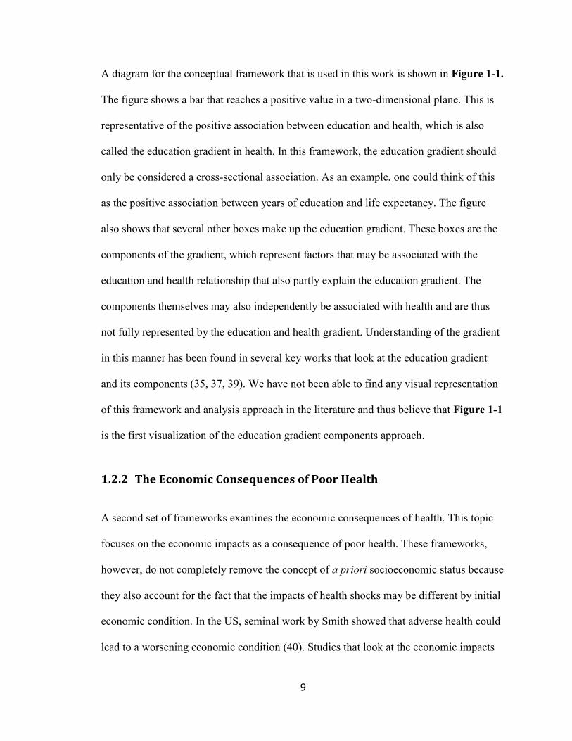
A diagram for the conceptual framework that is used in this work is shown in Figure 1-1.
The figure shows a bar that reaches a positive value in a two-dimensional plane. This is
representative of the positive association between education and health, which is also
called the education gradient in health. In this framework, the education gradient should
only be considered a cross-sectional association. As an example, one could think of this
as the positive association between years of education and life expectancy. The figure
also shows that several other boxes make up the education gradient. These boxes are the
components of the gradient, which represent factors that may be associated with the
education and health relationship that also partly explain the education gradient. The
components themselves may also independently be associated with health and are thus
not fully represented by the education and health gradient. Understanding of the gradient
in this manner has been found in several key works that look at the education gradient
and its components (35, 37, 39). We have not been able to find any visual representation
of this framework and analysis approach in the literature and thus believe that Figure 1-1
is the first visualization of the education gradient components approach.
1.2.2 The Economic Consequences of Poor Health
A second set of frameworks examines the economic consequences of health. This topic
focuses on the economic impacts as a consequence of poor health. These frameworks,
however, do not completely remove the concept of a priori socioeconomic status because
they also account for the fact that the impacts of health shocks may be different by initial
economic condition. In the US, seminal work by Smith showed that adverse health could
lead to a worsening economic condition (40). Studies that look at the economic impacts

10
of adverse health events have termed these events “health shocks”, which is a subset of
broader economic shocks, which may be due to individual level adverse events
(idiosyncratic) or broader level adverse events (covariate). Research on health shocks
have proposed that these are idiosyncratic events with exogenous properties that may be
used for understanding the causal impact of health on wealth (20, 21, 41).
To understand how adverse health events effect economic outcomes, there have been two
frameworks proposed. One of these was proposed by Russell, which establishes that poor
health can impact household wealth through direct and indirect costs (42). A similar
framework, published two years after Russell’s was proposed by McIntyre and colleagues
(43). This framework included the concept of direct and indirect costs but also described
specific coping mechanisms that households use in response to these costs (43).
Employing the McIntyre framework in research in Bangladesh has previously been done
as well (44). A modified version of the McIntyre framework was used to look at coping
for this dissertation (see Chapter 4). Coping strategies are divided into three main
categories: financial, demographic and behavioral, and ten individual coping strategies
are divided among the three categories. The modified framework is seen in Figure 1-2.
1.3 Study Objectives
The goal of this dissertation is to evaluate microeconomic aspects of NCDs in a rural, low
income area of Bangladesh with a long-running surveillance system. The work will
characterize the education gradient for NCDs and infectious diseases in this area and look
at the components of the education gradient such as income, occupation and marital

11
status. To look at the economic impacts of an adverse health event from an NCD, this
work will also use a matched cohort study and a newly developed statistical estimator to
attempt and measure the marginal relationship between an NCD death and being poor.
Lastly, the risk of being poor because of a health event likely occurs because of channels
of influence that cause a household to incur health expenditure and lose production
capacity. The third focus of this work will examine which coping strategies are used after
an NCD death and whether or not there are changes to household composition, defined as
the total number of household members as well as the total number of members
according to gender and age (male or female; child or adult). The specific research
objectives and sub-objectives are listed as follows:
1. To explore the education gradient from adult mortality in Matlab, Bangladesh.
a. Characterize the education gradient in mortality for adult NCD and
infectious disease deaths.
b. To explore the components of the education gradient and to what extent
factors related to wealth, occupation and marital status explain the
gradient.
2. To evaluate the economic impact on households from a health shock from an
NCD death in Matlab, Bangladesh.
a. To assess whether an NCD health shock leads to a higher risk of being
poor two years after the death according to three different measures of
economic status.
b. To examine the individual-level characteristics of the deceased that are
associated with a higher risk of being poor after an adult NCD death.

12
3. To evaluate the coping strategies that a household uses after a health shock from
an adult NCD death in Matlab, Bangladesh.
a. To identify which coping strategies households use after an adult NCD
death.
b. To explore what individual and household-level characteristics are
determinants for using certain coping strategies.
In the first objective, the hypothesis is that there will be an education gradient in NCD
mortality. The component of wealth is hypothesized to contribute the most to the gradient
in education, however, given the informal economy and overall low levels of wealth in
Matlab, there may be large roles for non-monetary components of the education gradient.
For objective #2, the hypothesis is that a death to a prime age adult member of the
household from NCD will lead to a higher risk of a household reporting being poor in the
two year period after the death. Households with a death to prime age member, male
member, head of the household or member with a higher level of education will be at the
highest risk of being poor.
Objective #3 adds to the picture the spectrum of coping strategies that households use
after a death. The hypothesis in this analysis is that households will engage in several
types of activities to smooth consumption after the shock from a death. Those households
where the death represents a more severe economic impact, such as the death to a prime
age member may attempt to replace the lost household member. Coping strategies may
have the largest negative impacts for poorer households if they are not able to smooth
consumption after a death and thus contribute to a cycle of poor health and poverty.

13
The three objectives of this work have to do with understanding the economics related to
the NCD burden in adults in low and middle-income countries in terms of the impacts at
the household level and how households may experience differing impacts based on the
characteristics surrounding the death and the household’s level of resources. The
organization of the rest of the thesis document is detailed in the following section.
1.4 Organization of the dissertation
The remainder of this dissertation is organized as follows:
Chapter 2: Explores the first objective looking at the education gradient in
mortality for infectious diseases and NCDs in Matlab over a 24 year period using
demographic surveillance data and periodic socioeconomic status census data.
The contribution of each of three components of this gradient are evaluated
according to sex and cause of death.
Chapter 3: Explores the wealth impact of having a shock from an NCD death in
Matlab. This is done with a new survey and matched-cohort study. A marginal
estimate of the risk of being poor is developed using a regression standardized
estimator specifically for matched cohort designs.
Chapter 4: Explores the economic impact from an NCD death through the coping
mechanisms that households use after the death. Individual and household-level
determinants of coping are explored and a difference-in-difference analysis is
used to examine coping in terms of human capital replacement.
Chapter 5: Concludes the thesis and offers final policy messages.

14
The main tables and figures for each paper appear at the end of each chapter. Additional
tables and figures are included in the last sections of the document in the appendices.
1.5 Figures for Chapter 1
Figure 1-1 Conceptual Framework for the Education Gradient in Health

15
Figure 1-2 Conceptual Framework for the Economic Consequences of Poor Health

16
Chapter 2. The Education Gradient in Adult Non-Communicable Disease and Infectious Disease Mortality: Are there Relevant Differences?
2.1 Abstract
This study attempts to gain understanding of the education gradient in adult mortality in a
low and middle-income country where there is a changing burden of disease from one
dominated by infectious diseases to one dominated by non-communicable diseases
(NCD). The education gradient in adult mortality, which is the positive association
between years of schooling and survival, is identified in Matlab, a rural area of
Bangladesh that has seen improvements in female education during the years 1982 to
2005. This work also explores the components of the education gradient in mortality for
both sexes and for deaths from both NCDs and infectious diseases. Cox proportional
hazards regression is used to examine the education gradient in NCD and infectious
disease mortality for three prospective five year periods beginning in 1982, 1996 and
2005 in Matlab. Component variables of wealth, occupation and marital status are
individually added to the base model to assess how much they contribute to the observed
education gradient in mortality. For females, an extra year of education significantly
reduces mortality from NCD by 7% and infectious disease by 12% (hazard ratios of 0.97
and 0.88). For males, an extra year of education provides a reduction in NCD and
infectious disease mortality of 2% and 8% (hazard ratios of 0.98 and 0.92). These
gradients mean that if everyone in Matlab were to achieve a level of primary education,
close to 2,600 deaths would be averted in the time period of this study. For the
components of the education gradient, marital status explains the highest portion for both

17
infectious disease and NCD mortality, followed by wealth and then occupation. These
three components account for a larger portion of the gradient in males than females, but
females show the steepest education gradients in mortality overall. With calls for more
services for the prevention and treatment of NCDs in low income settings, there is a role
for education in addressing the NCD burden. In Matlab, an increase in the levels of rural
female education is associated with the saving of many lives, but the levels of education
remain very low and education for men has been stagnant for several decades. Continued
investment in education will prevent deaths and become more important for NCDs, in
absolute terms, as the burden from NCDs rises. Policies should consider how access to
social-psychological resources in addition to economic resources are improved through
education, when attempting to identify those who are vulnerable to mortality and poor
health. This study in rural Bangladesh provides a model for understanding the education
gradient in health for low-income countries with changing disease patterns.
2.2 Introduction
This study attempts to gain understanding of the education gradient in health in low and
middle-income countries where there is a changing burden of disease from one
dominated by infectious diseases to one dominated by non-communicable diseases
(NCD). The “education gradient” is the consistent positive relationship between
education and health, which has been shown to reliably exist in many settings (23, 32,
37). This relationship has been well-studied for different outcomes of health in high
income countries but less work has been done in low and middle-income countries,
especially for adult health. Much of the education gradient work that has been done in

18
low and middle-income country settings deals with issues in child health and HIV/AIDS,
with less emphasis on issues related to adult NCD health (45, 46).
In the past decades, Bangladesh has been steadily developing economically, which is
seen by a consistent upward trend in the country’s per capita gross domestic product
(GDP) (Figure 2-1) (47). Additionally, the country has had a declining poverty rate
nationally and for the rural population (Figure 2-2) (48). The country has also begun to
address the issue of low education by making investments in rural female education (49).
Since the mid 1990’s, there have been successful efforts to increase school attendance for
females and data from one rural area shows a near doubling of the years of education that
females complete from 1982 to 2005 (Figure 2-3). In contrast, rural male education
levels have remained stagnant, so any increase in overall levels of education needs to
account for the differences by sex.
Along with economic development, Bangladesh is also undergoing an epidemiologic
transition, with improvements in infectious disease mortality and an increasing portion of
the burden of disease coming from NCDs (Figure 2-4). Gaining an understanding of the
education gradient for Bangladesh is important to evaluate how investments in health
services and education may contribute to improved health overall. In the rural area of
Matlab, many years of investments in child health, maternal health and family planning
services and environmental improvements have led to a rapid decline in the burden from
infectious diseases and a corresponding increase in the burden from NCDs (5). Figure 2-
5 and 2-6 show the mortality rates in Matlab for both infectious diseases and NCDs for

19
the whole population by level of education, classified as either high or low. The figures
show a clear health benefit to education for lowering mortality rates for each disease
category, regardless of whether the overall disease rates are increasing or decreasing.
The Matlab upazila (sub-district) is located in the state of Chandpur and has a population
of a quarter of a million people. Since 1966, it has been a site for demographic
surveillance and public health programming (even before the establishment of the
modern country itself). Led by the nonprofit organization, the International Center for
Diarrhoeal Disease Research in Bangladesh (icddr,b), the area has implemented programs
addressing issues of cholera, access to clean water and family planning. Both the icddr,b
and the Bangladeshi government currently operate hospitals that provide free maternal
and child health services to the Matlab population.
The well-established positive relationship between education and health provides
justification for investments in education as a health improving strategy (50). In the social
sciences literature, there have been attempts to examine the causal effects of education on
health using quasi-experimental approaches with education modeled exogenously,
meaning it is assumed that one’s education does not depend on one’s health (30, 51, 52).
These studies have identified settings where econometric designs such as regression
discontinuity and instrumental variables estimation can be used to obtain the exogenous
effect of education on improved health.
In the absence of the right conditions for making causal conclusions, there have also been
attempts to understand the components of the education gradient, which may shed light
on the mechanisms explaining the positive education and health relationship. The

20
components of the gradient are defined as the mechanisms through which education
affects health. Previous work has identified these components and established
frameworks to examine how each one contributes to the positive education and health
relationship (32, 35, 37, 53). The main components typically include: economic
resources, social-psychological resources, prices, cognitive abilities, personal
endowments, health behavior, environmental factors and tastes (33, 35, 37). This research
in Matlab, lacking an exogenous measure of education, adopts this second approach to
explore the components of the observed education gradient in mortality.
The aim of this study is to identify the education gradient in mortality in a rural, low
income country setting in Bangladesh and to explore the contribution of three
components of this gradient, wealth, occupation and marital status. The education
gradient is evaluated in adult mortality by sex and by broad category of cause of death:
infectious disease and NCD. By comparing the two categories of diseases, the work sheds
light on unobserved components of the education gradient as well, which may help to
design better policies. For example, does education have a larger effect for those affected
by NCDs or infectious diseases and should education interventions be targeted to those
with who are vulnerable in terms of economic resources or social-psychological
resources. This research is especially relevant given the emerging burden from NCDs in
Matlab and other countries that are undergoing an epidemiologic transition.

21
2.3 Literature Review
2.3.1 Education and mortality relationship in LMICs and Bangladesh
Since the seminal work of Kitagawa and Hauser in 1979 looking at mortality differentials
in the United States by level of education, there have been many studies to further
understand the education and mortality relationship (23). Using country data from the US
and Western Europe, researchers have addressed questions related to the education and
mortality relationship according to age, sex, race and other sub groups where the
relationship may be important for understanding socioeconomic status and health (52, 54,
55).
In low and middle-income countries, however, there has been much less research looking
at the education gradient in mortality. This may be due to the lack of data for these
settings or that the levels of education remain very low. Suppressed levels of education in
low and middle-income countries have been hypothesized to reduce the relationship
between education and health, yet researchers still see gradients when looking at issues
such as HIV/AIDS mortality, parental education gradients in child mortality and child
education gradients in child mortality gradients(25, 51, 56-59). In recent years, as NCDs
have emerged as a global health issue, there have also been more studies looking at
education gradients for adult health in low and middle-income countries that specifically
looking at non-communicable diseases (46).
The long-running surveillance site in Matlab, Bangladesh has been collecting information
on mortality and education since the 1970s and previous researchers have used this data
to look at the differences in mortality by education. Using Matlab data from 1974-1977,

22
one study found an education gradient in mortality in Matlab when dividing education
into three categories: none, primary and secondary, according to the education of the
head of the household or the highest education of anyone in the household. In each case
the mortality rate ratio of the lowest educated to highest educated ranged from 1.9 to
close to 3 (60). Utilizing the same Matlab data up to the year 1996 to study the survival
of adult females, another study used a binary education variable and found that women
with any years of education had a 1.6 times survival advantage over those with no formal
education (61). A more recent estimate using Matlab data in the years 1996 and 2005
came to a similar conclusion, finding that literate adults were 1.46-1.61 times more likely
than illiterate adults to survive in the subsequent three year period (62).
2.3.2 Causal literature on the education and health relationship
In the field of Economics, some of the initial ideas relating education to health were put
forward by Gary Becker (63). These were further developed by Grossman’s use of
education in the health production function and subsequent review looking at the non-
market outcomes of education (50). An important point is that education, or knowledge
capital, may be endogenous to health. This means that there may be reverse causality
where health leads to better schooling or there may be an omitted variable that explains
both education and health (64). One popular explanation for the third variable hypothesis
was proposed by Fuchs, postulating that time preference may be the omitted third
variable explaining both education and health (65).
There are several quasi-experimental research techniques that may be able to account for
some of the endogeneity when evaluating the causal effect of education on health. These

23
include: using lagged health variables, using the differences in health of twins or sibling,
using instrumental variables or using regression discontinuity that examines the effect of
education around a discrete cut-point or policy change (30, 50). While these techniques
have been used more frequently in developed country settings, they are beginning to be
used in developing country settings as more and better data becomes available (30, 51,
52).
One important conclusion from the causal literature on the education and mortality
relationship is an understanding of the size of the effect. That is, how much health, in
terms or better survival, does one extra year of schooling buy. This is difficult to discern
given the variety of study populations, research designs and methods for measuring
education and mortality. Regardless, the results reported that there is generally a less than
10% reduction in five or ten year mortality in adults for each extra year of schooling. For
example, for US data, one study finds a 3.6% reduction in ten year mortality for an extra
year of education and another finds a 7 to 9% reduction in five year mortality for each
additional year of education (39). For lower and middle-income countries, there was no
quasi-experimental results found for adult mortality, however, using instrumental
variables in Indonesia, one study finds a near 12% reduction in the total number of
children who die for each additional year of parental education (51). Clearly there is
variation in the gradient depending on the characteristics of the mortality cause, time
period, age and region of interest and an understanding of the education gradient in
mortality for adults in low and middle-income countries is warranted.

24
2.3.3 What are the components of the gradient
In addition to understanding the causal effect of education for health, it has also been
important to understand the components that make up the gradient. While not causal in
nature, this research provides insights into why the education gradient exists, and this
understanding may be used to design better policies for health improvement (66).
In the sociology literature, Ross and Wu set a framework of explanatory categories of
work and economic conditions, social-psychosocial resources and health lifestyle (35).
Economics frameworks understand the education gradient in similar terms though they
add economic constraints of income, prices and access that may explain the gradient (33).
Additionally, there has been an addition of cognitive ability and non-cognitive abilities
(such as ability to act) that have been explored as well (37, 38, 67).
2.3.3.1 Wealth & Occupation
The first component that is usually mentioned in most frameworks is that of economic
resources. This may be measured with a variable for income (or wealth). The component
for economic resources usually explains a large portion of the gradient, and in empirical
research, has been shown to be the most important component of the gradient (37).
Lower education is associated with lower income and vice versa for higher education
(68). Cutler explains that income can effect health through two channels: more income
can buy more health-improving goods such as healthcare or health insurance and more
income can increase consumption, which leads to a higher utility for living to older ages.

25
In this sense, income can be thought to be an indicator of command over and access to
resources (37).
Income is usually thought to explain a large portion of the education gradient in health. In
a review of several datasets for the effect of economic resources on the education
gradient in the use of prevention, Cutler finds that economic resources overall explain
20% of the gradient and it could even explain as much as 32%, depending on the dataset
that is used (37).
Occupational status may also play an important role. One study that combines work and
economic conditions found that up to 59% of the gradient in self-rated health can be
explained (35). Measuring economic resources through occupation is not new and has
been famously done in the Whitehall II study to look at social gradients in mortality (22).
In addition to the relationship with income, lower education may lead to a worse
occupation status which may then impact mortality (68, 69).
2.3.3.2 Marital status
In addition to the variables for economic resources, a variable for social, or social-
psychological support is also thought to explain part of the education gradient. Marital
status has been used as a proxy for such types of support and has been found to be an
important type of informal support that may work in addition to formal support
mechanisms (e.g. workplace programs) (35, 70). The effect of marital status is thought to
be related to higher levels education and more stable marriages are thought to be an

26
important “non-pecuniary” impacts of more schooling (71). In the reverse direction,
marital may also be a critical determinant of mortality as well (72).
In one study in the United States, variables for marital status, income, household size and
rural/urban status, when combined, were found to explain between 20-50% of the
education gradient in mortality (39). In Bangladesh, marital status has also been
previously found to be an important determinant of mortality (35, 73). Although, we are
cautious about interpreting marital status as an accurate proxy for social support given
that marital status in rural Bangladesh is also determined by different cultural practices
than it is in other developed countries.
2.3.3.3 Other Components of the Gradient
Prices are thought to influence the education and health relationship if those with more
education are economically better off and more price elastic. That is, those with more
education may be more likely to reduce unhealthy behaviors that have a cost (37). The
evidence for this component is weaker, however, and there have also been studies
showing that the less educated are more price elastic (74). Prices, however, in Matlab are
thought to be held relatively constant for the entire population and thus are considered to
not have the variation necessary for examination.
Cognitive abilities are another element that may contribute to the education and health
gradient. Those that have higher abilities may be more efficient at producing health (50).
The data requirements to look at cognitive ability are certainly more intense and less
work has looked at this component; however Goldman and Smith find a strong effect of

27
cognitive ability by including an intelligence score in their model with years of schooling
(75).
The previous two components of the gradient, prices and cognitive ability, are not
evaluated in this work due to data limitations, but prices are assumed to play a minimal
role in the education gradient. Cognitive ability is more problematic, given that it may
explain a potentially large part of the gradient, and may be an important element that
cannot be accounted for (31). In addition to these two components, there are elements of
personal endowments and environmental conditions that could also explain the gradient.
2.3.4 The Education gradient by infectious and non-communicable
disease
Since there is only data available for the three components of wealth, occupation and
marital status, the exploration of the education gradient by broader cause of death
category, NCD and infectious disease, is undertaken to shed further light some of the
unmeasured components. In essence, there may be some important characteristics of
NCDs and infectious diseases themselves that could lead to a better understanding of the
gradient and its components.
There has been no previous work, to the best of our knowledge, which dichotomizes
cause of death according to these categories when exploring the education gradient in
health. Perhaps the closes attempt at this was done by Montez and colleagues who
divided causes of death into those that had behavioral determinants (such as smoking
causing chronic lung disease) and non-behavioral components. This classification

28
roughly followed a stratification by NCD and infectious diseases where the behavioral-
related causes equate to the NCD category. The results of this study find that diseases
with behavioral components explain more of the education gradient in males than for
females, though the authors do note the limitations of making conclusions about the
component of behavior simply by the cause of death (70).
Other previous work has also highlighted the education gradient in terms of the
behavioral risk factors that lead to increased NCD burden. One study looking at smoking
concluded that a steeper education gradient (greater difference in health outcomes) may
be found when knowledge about risk factors emerges because education leads to a more
efficient use of knowledge (45, 50). For developed countries, there have also been studies
concluding that the education gradient for chronic diseases will be larger because the
more educated are better able to manage complex prevention and treatment for chronic
conditions (76). This conclusion has been made with other health interventions such as
the use of more information intensive strategies for contraception (77). An important
point, however, is that the access to information is found to be very important for an
education gradient in health to emerge (45). For NCDs in Matlab, where there is very
little access to information about NCDs and related risk factors, there may be a narrowing
gradient (smaller relative difference) in NCD mortality, as mortality rates rise.
On the other hand, they may also have a steep education gradient in infectious disease
mortality in a setting such as Matlab. While infectious disease mortality is rapidly
declining, from a relative perspective, the gradient could be getting larger. There has been
some evidence that large-scale public health programs, such as the one in Matlab are

29
inequality-enhancing (78, 79). Although services are generally focused on the infectious
disease burden, the poorest are the least likely to receive services even in a situation
where services are provided freely. There has been some evidence for this in high income
countries where universal access does not reduce inequalities (80).
To summarize, most research on the education gradient in mortality has been conducted
in developed countries, though there is indication of a gradient existing in developing
countries as well. In the causal literature, quasi-experimental designs have found that
investments in education will lead to significant improvements in health. This effect may
work through several components related to economic condition, social-psychological
resources, prices, cognitive ability and other factors. Of these, economic condition and
cognitive ability have been found to play a large role in explaining the gradient but so has
social-psychological resources, measured by marital status. No studies have examined the
education gradient in mortality according to broad cause of death categories such as NCD
and infectious disease, but there has been some work in developed countries showing that
the gradient in NCD mortality will be significant because of education’s relationship with
health behaviors and efficient use of information. This study attempts to fill this gap in
the literature by evaluating the education gradient in mortality gradient in a rural, low
income area, looking at components related to economic and social-psychological
resources as well as broad categories for cause of death.

30
2.4 Data
2.4.1 General data
This study uses census data with individual identification numbers to link death
certificate information with socioeconomic and household characteristics in Matlab. Data
from the Matlab surveillance system is used for the population in 1982, 1996 and 2005.
These three time points are when wealth surveys were conducted in Matlab and provide a
cross-sectional picture of socioeconomic status at those times. The follow up time for
mortality information is limited to five years. Longer follow up periods would not capture
significant changes in variables such as household wealth and marital status that are
changing in time and may affect conclusions about the relationship between education
and mortality. This approach is consistent with previous examinations of socioeconomic
status and mortality in Matlab and other settings (60-62).
The study population includes all those who are alive, aged 15 years or older at the
beginning of each year in Matlab in 1982, 1996 and 2005, following them for
outmigration and death. Using an age cut-off of 15 years ensures that the majority of the
selected population has completed education. This is a common cut-off for research
looking at effects of adult education in developing countries, and lower than the usual
cut-off for developed countries, which is usually 20 to 35 years old (34, 81).
2.4.2 Primary Dependent Variable - Mortality
Mortality was coded as a binary variable for whether someone experienced a death in the
follow up period or not. Deaths were broken down into broad disease categories for NCD

31
and infectious disease according to the death classification scheme used by the
surveillance program in that year. The NCD category did not include any injuries, both
intentional and unintentional and all causes of death from maternal and reproductive
causes for females were excluded.
Notably, for each of the three periods, a different cause of death classification system was
used. In 1982, the cause of death was documented by the interviewer at the time of
collecting the information about the death. By 1996, the surveillance team used verbal
autopsy methods for classifying death into 98 separate causes. In 2005, the verbal
autopsy system was refined to classify cause of death according to the International
classification of disease version 10 (ICD-10). The categorization of the causes into two
broad categories is an attempt to reconcile these differences in assigning specific causes
of death in each period. This approach has been used previously when describing cause
of death information for Matlab (5, 62).
2.4.3 Primary Independent Variable - Education
Education was measured as a continuous variable for the years of education completed,
ranging from zero to sixteen, for the deceased individual. For sensitivity analyses, a
categorical education variable based on the years of education completed with categories
for no education, 1-5 years completed, 6-10 years completed and 11 or more years
completed was used (82). These categories are consistent with the education system in
rural Bangladesh. Additionally, this analysis only uses a measure of year of formal
schooling completed. Children in Matlab may attend religious schools for all or part of

32
their education, but consistent with previous work in Matlab, we separate formal
schooling from religious schooling (73).
2.4.4 Further Independent Variables - Exogenous Controls
Each of the models specified in equations 1-5 include a set of control variables. These
variables are: age, religion, household size, birth cohort and census year. These variables
are not influenced by years of formal education and are considered exogenous to the
education and health relationship.
Individual age is included as a continuous variable and age is also examined as a
categorical variable to control for birth cohort effects. Following previous work in
Matlab, we use age groups of 15-40, 40-59 and 60+ to describe groups of young, middle-
aged and older adults (6, 62). A further categorical variable is included for religion,
whether someone is Muslim, and dummies are generated for the three time periods of
interest in order to account for long-term trends. A similar dummy-variable approach has
been used previously to examine long-term mortality trends in Matlab (61).
2.4.5 Components of the Education Gradient
This study looks at three components of the education gradient. The first two are wealth
and occupation, which are an indicator of one’s economic resources. The third
component is marital status, which has been proposed as a measure of social-
psychological resources in developed country settings and which may play a role in
developing country settings as well. Other components of the gradient such as prices,
health lifestyle, cognitive abilities and non-cognitive abilities are either assumed to be

33
constant or unobserved. In our data, wealth is measured at the household level and
occupation and marital status are individual-level measures.
2.4.5.1 Wealth
Wealth was measured with an ordinal quintile scale with a one representing being very
poor and a five representing being very rich. The quintile was calculated by the
surveillance system for each household in the base years using principal component
analysis (PCA) for a list of durable household items as well as characteristics that
included land ownership, home building materials and type of latrine and water source
utilized (83). The socioeconomic status instruments were standardized for the years 1996
and 2005, but was slightly different for the year 1982, primarily using a smaller list of
durable assets. However, given the large number of assets listed for each year and the
degree of overlap in assets used, this measure is considered to be a consistent measure of
wealth for each time period.
2.4.5.2 Occupation
Occupational status was classified into seven main groupings based on a review of the
main economic activities in the region and previous literature (84). The occupational
categories capture key classifications made by a previous study in rural Bangladesh and
by the Bangladesh Bureau of Statistics (84, 85). The surveillance system in Matlab used
different occupational groupings for the year 1982 than it did for 1996 and 2005 so such a
standardization was necessary. In contrast to previous studies, this research includes a
category for homemaker or housewife to be able to assess the effect of this dominant
female occupation on female mortality (58, 86). A category for being a student is also

34
included despite its clear endogeneity with the effect of education. This has been done in
previous studies in Bangladesh, and it is assumed that given the overall low levels of
education in the area that most of the gradient for education comes from those with lower
levels of education who are not likely to still be students (84).
2.4.5.3 Marital Status
Marital status includes three categories including: single/never married, married and
widowed/divorced. This categorization has been previously used for research in Matlab,
though it may fail to capture the effects of individuals who marry multiple times and
experience variable states of marital status over time. In this analysis, the most recent
listing of marital status of an individual is used prior to a mortality event or censoring due
to outmigration.
2.4.6 Data limitations
As mentioned above, there may be an issue with the classification of deaths into broad
categories because the process for assigning causes of death in Matlab varied
dramatically from 1982 to 2005. Collapsing the causes into broad categories of death is
an attempt to account for this. The errors in assigning cause of death are less severe in
this study if such errors only occur within categories. This has been proposed as a likely
scenario by previous work in Matlab (5). There may still be problems; however, since in
each year individuals with various levels of medical expertise were tasked with assigning
the causes of death.

35
There may also be an issue with the large number of unknown deaths that are found in
the earliest time period, 1982. For this early period there were 404 unknown male deaths
and 376 unknown female deaths. Looking at the average age of death from unknown
causes showed that in males, these fell near the “young NCD” deaths with a mean of 59
years. This, for example, is the same as the mean age for the known Cancer deaths. This
same pattern was seen for unknown female deaths, with the mean age of unknown death
being around 53 years, which is close to the 54 year old mean for female cancer deaths.
Next, when looking at the gradients for just the unknown causes, in males, the gradient
was closer to the NCDs (education coefficient = -0.03). For females, this was opposite,
with the gradient for the unknowns being quite large and closer to the infectious disease
estimate (education coefficient = -0.24, unadjusted). Further work may be needed to
determine how these unknown deaths may bias the results.
Another limitation is the measurement of the variable for education. Using only year of
education completed does not provide any indication of the quality of education. A
further limitation of the education variable may be that low levels of education overall
hinders uncovering the true relationship between education and health (58). This study
assumes that education is linear in health, but there may be important differences in this
relationship at different education levels. This relationship has been explored in studies in
the (34, 87). In Matlab, there are very few individuals at the highest educational levels,
and many people with zero years, meaning that much of the health benefits from
education are a result of completing just a few years of education. This is further explored
by collapsing education into a binary variable for any years of schooling and into a
categorical variable for the different schooling levels (none, primary, secondary, post-

36
secondary). The results are not shown but are consistent with those presented for year of
education completed.
Using wealth is one of the strengths of this analysis since income may be subject to short-
term fluctuations, unrelated to education (31). The use of an asset-based wealth quintile is
also a standard measure of wealth in developing countries when income and consumption
data are not available (88).There may also be limitations to using asset- based wealth;
however, as the PCA based quintile may mask important heterogeneity of wealth levels
and access to resources between household members. This is especially worrisome for
females, given their lower status in Matlab society.
The variable for occupation could also have drawbacks. The variable for occupation
(one’s primary economic activity) in the Matlab surveillance system is coupled with that
for employment status (whether one is working) so the effect of having an occupation in
of itself may be confounded. Employment status would be a better variable to use if it
was available, since if one is not working, this may be due to ill health prior to imminent
death (35, 69).
2.5 Econometric framework
The association for the effect of education on adult, chronic disease death was analyzed
using a multivariate cox proportional hazard regression model separately for each sex and
each major broad category of cause of death, NCD and infectious disease. The equation is
specified as follows:
𝑙𝑜𝑔 ℎ𝑖(𝑡) = 𝛼(𝑡) + 𝛽1𝐸𝑑𝑢𝑖 + 𝛽2𝑋𝑖 (1)

37
Where hi(t) is the hazard function for individual i at time t, 𝛼(𝑡) is the baseline hazard,
Edui is year of education for individual i, the main independent variable of interest, and
𝛽1 is the coefficient on year of education, which represents the education gradient. 𝑋i
represents assumed independent variables of interest of age, religion, household size,
birth cohort, and census year.
The models employed right-censoring and used the Efron method to account for tied data.
Survival time is calculated from the time of the base year census and age is included in
the model to derive the age-adjusted hazard of mortality (34, 89, 90). All standard errors
are clustered at the household level.
To examined the relationship of education with the hazard of mortality, four
specifications of the model were run: with education as the only independent variable
(not shown), as a reduced form model with education and exogenous controls (equation
1), as a reduced form plus each of the components added individually (equations 2-4) and
as a reduced form plus all of the components added at once (equation 5) (39). The
exogenous controls for the reduced form model include variables for age, religion,
household size, birth cohort and census year. The explanatory power of the component
variables of wealth, occupation and marital status were then assessed in models 2, 3 and 4
below, with 𝛽3 representing the coefficient on the component variable:
𝑙𝑜𝑔 ℎ𝑖(𝑡) = 𝛼(𝑡) + 𝛽1𝐸𝑑𝑢𝑖 + 𝛽2𝑋𝑖 + 𝛽3𝑊𝑒𝑎𝑙𝑡ℎ𝑖 (2)
𝑙𝑜𝑔 ℎ𝑖(𝑡) = 𝛼(𝑡) + 𝛽1𝐸𝑑𝑢𝑖 + 𝛽2𝑋𝑖 + 𝛽3𝑂𝑐𝑐𝑢𝑝𝑖 (3)
𝑙𝑜𝑔 ℎ𝑖(𝑡) = 𝛼(𝑡) + 𝛽1𝐸𝑑𝑢𝑖 + 𝛽2𝑋𝑖 + 𝛽3𝑀𝑎𝑟𝑟𝑖 (4)

38
The final model that included all independent variables at the same time is given by the
following equation:
𝑙𝑜𝑔 ℎ𝑖(𝑡) = 𝛼(𝑡) + 𝛽1𝐸𝑑𝑢𝑖 + 𝛽2𝑋𝑖 + 𝛽3𝑊𝑒𝑎𝑙𝑡ℎ𝑖 + 𝛽4𝑂𝑐𝑐𝑢𝑝𝑖 + 𝛽5𝑀𝑎𝑟𝑟𝑖 (5)
To understand the degree to which the education gradient in mortality is explained by the
three explanatory variables of interest, we used an approach where the percent reduction
in the coefficient on education was calculated with the addition of the variable of interest
individually to the base model. For example, for the addition of wealth in equation 2, the
percent explanation of the education gradient was calculated as: [(𝛽1𝑀𝑜𝑑𝑒𝑙 1 −
𝛽1𝑀𝑜𝑑𝑒𝑙 2)/𝛽1
𝑀𝑜𝑑𝑒𝑙 1] ∗ 100], where 𝛽1𝑀𝑜𝑑𝑒𝑙 1 is the coefficient on the variable for
education for model 1. This was then repeated for models 3, 4 and 5, each time using
model 1 as a reference. This method has been employed by others when evaluating the
degree to which an added variable explains the relationship between the primary
dependent and independent variables of interest (34, 35, 37, 41).
As the education gradient in mortality is represented by a rate ratio, it represents a
relative effect and a further step is needed to understand the absolute effects of the
education gradient (32, 33, 91). After the cox proportional hazard models were estimated,
the expected number of deaths, as a predicted value, were obtained assuming a scenario
where everyone in the population of Matlab completed primary education, which was 5
years. These deaths were then subtracted from the observed number of deaths in the
pooled data to obtain an estimate of the deaths that could be averted if everyone
completed this basic level of education.

39
2.6 Results
Descriptive information for the entire study population stratified by sex is provided in
Table 2-1. The table provides information pooled for all three years.
2.6.1 The link between Education and the Components of the Gradient
Initially, ordinary least squares regression was used to examine the general relationship
between year of education and variables for marital status, occupation and wealth. These
models were set up according to the following specification:
𝑍𝑖 = 𝛽0 + 𝛼𝐸𝑑𝑢𝑖+ 𝛽𝑘𝑋𝑘 + 𝜖𝑖 (6)
In equation 6, 𝑍𝑖 represents the component of interest, either wealth, occupation or
marital status. The variable 𝐸𝑑𝑢𝑖 represents the year of education for individual i with 𝛼
being the coefficient for the relationship between a change in year of education with a
change in the component. The vector 𝑋𝑘 represents independent control variables at the
individual and household level and 𝛽𝑘 is a vector of their corresponding coefficients. The
control variables are: age, religion household size, birth cohort and census year. This
preliminary analysis provides an estimate of R2 to describe how the observed variation in
wealth, occupation and marital status is explained by education.
Equation 6 was run for the pooled dataset and separately for males and females with
results shown in Table 2-2. Models were also run for each of the time periods
individually and there were no large changes in the R2 values or explanatory rank of the
coefficients by year. For both sexes, education is significantly positively associated with

40
wealth, occupation and marital status and the largest coefficient on education is seen
when wealth is the dependent variable. Examining the R2 values, education explains the
most variation in wealth, (R2 0.20 for males and 0.22 for females). Education explains
slightly less of the variation in marital status, with an R2 value of 0.18 for both sexes.
Education explains the least amount of variation in occupation, with an R2 value of 0.04
and 0.05 for males and females.
2.6.2 Overall education gradient in mortality
The results for the overall education gradient in mortality for both sexes and causes of
death for the pooled data is shown in Table 2-3. The gradient in education is measured
by the coefficient on the variable for year of education from the reduced form equation 1
(again: 𝑙𝑜𝑔 ℎ𝑖(𝑡) = 𝛼(𝑡) + 𝛽1𝐸𝑑𝑢𝑖 + 𝛽2𝑋𝑖).
For females, the gradient in both causes is significant and shows an extra year of
education is positively associated with a decline in mortality (hazard ratio less than one).
For female NCD mortality, an extra year of education is associated with a 7% reduction
(HR = 0.93) and for infectious disease mortality and an extra year of education is
associated with a 12% reduction (HR = 0.88) in mortality. In absolute terms, this
education gradient would result in 689 averted female NCD deaths and 1,275 averted
female infectious disease deaths if every female in Matlab had a primary level of
education. This represents 21% and 55% of the NCD and infectious disease deaths that
were observed over the time period.

41
In males, the gradient in both cause of death categories also shows a positive relationship
with health and both are significant. Male NCD mortality is reduced by 2% (HR = 0.98)
for every year of education completed and male infectious disease mortality is reduced by
8% (HR = 0.92) for every year of education completed. This means that if every male in
Matlab had a primary level of education, 167 NCD deaths and 505 infectious disease
deaths would be averted, representing 4% and 20% of the observed deaths from these
causes in the time period.
The steepest education gradients, which is a relative effect, and the largest number of
deaths averted, the absolute effect, are both seen in infectious disease mortality. By sex,
the largest relative and absolute effects are seen for females.
2.6.3 Components in the education gradient
Table 2-4 gives the results when adding the three components of wealth, occupation and
marital status to the reduced form base model for female mortality. When adding all three
of these components, the education gradient is reduced by 59% in NCD mortality and by
27% in infectious disease mortality and remains significant for both causes of death. With
all three components accounted for, an extra year of education provides a 3% reduction in
NCD mortality (HR = 0.97) for females and a 9% reduction in infectious disease
mortality (HR = 0.93) for females. This equates to 361 total NCD deaths averted and 732
total infectious disease deaths averted over the time period, which represents 11% and
31% of the total observed deaths.

42
When adding the components to the reduced form base model individually, wealth
reduces the education gradient in NCD mortality by 14% and the gradient in infectious
disease mortality by 11%. Occupation showed a minimal effect, reducing the education
gradient in NCDs by 1% and by less than 1% for infectious diseases (denoted NA).
Marital status reduced the education gradient by the largest amount in female NCD and
infectious disease mortality reducing the gradient by 52% in the former and 16% in the
latter.
In Table 2-5, the results are shown when adding the three components of wealth,
occupation and marital status to the model for male mortality. For NCD and infectious
disease mortality, when adding all three of the components, the education gradient is
completely reduced in male NCD mortality (100% reduction) and no longer significant.
In infectious disease mortality, the education gradient is 49% reduced when all three
components are added. In these models, completing an extra year of education provides
no mortality benefit for male NCD mortality (HR = 1.00) and a 4% reduction in
infectious disease mortality (HR = 0.96). This equates to 261 averted infectious disease
deaths in the time period, 11% of the observed deaths, and no averted deaths from NCDs.
Table 2-5 also shows the amount that each component individually explains the
education gradient in male mortality. For NCD mortality, wealth explains 48% of the
gradient while wealth only explains 20% of it in infectious disease mortality. Occupation
explains 19% of the gradient in NCDs and a similar amount, 21%, in infectious diseases.

43
Adding marital status results in the entire gradient being explained in NCDs mortality
and 21% of the education gradient in infectious disease mortality.1
In all, the three components explain a large portion of the education gradient in NCD
mortality, explaining 59% of the gradient for females and the entire gradient for males.
The three components explain less of the gradient in infectious disease mortality, 27% for
females and 49% for males. Marital status explains the most for any sex and cause, but
shows and especially large effect for NCD mortality. Wealth and occupation still explain
a large part of the gradient for male mortality, but for females these components explain
much less.
2.7 Discussion
This study identified the education gradient in mortality for the rural, low income area of
Matlab, Bangladesh and explored how the components of the education gradient in
mortality differ by sex and cause of death category. The education gradient in mortality
was examined for three prospective five year periods beginning in 1982, 1996 and 2005.
Component variables of wealth, occupation and marital status were individually added to
the base model to assess how much they contribute to the education gradient.
The education gradient overall shows that there is a range of a 2 to 12% reduction in
mortality per year of schooling completed in both sexes depending on whether NCDs or
1 To test this further, we also run models restricting the age of the sample to different cut points. When
removing those who are aged older than 65, marital status explains 80% of the gradient in male NCD
mortality. This may be a result of a steeper education gradient seen for the restricted group if the “age-as-
leveler” theory holds in the Matlab population 92. Dupre ME. Educational differences in age-related
patterns of disease: reconsidering the cumulative disadvantage and age-as-leveler hypotheses. Journal of
health and social behavior. 2007;48(1):1-15. Epub 2007/05/05..

44
infectious diseases are being looked at. The gradient is steeper for females, meaning that
an extra year of education completed confers a larger reduction in mortality. By
simulating a situation where all females achieve a level of primary education, the result
show that the relationship between education and mortality would avert 21% of the NCD
deaths and 55% of the infectious disease deaths that were observed. The steeper gradients
seen in females is interesting given that in settings such as the US and Western Europe,
the opposite is typically seen (55, 70). This is consistent with theories of gender bias in
patriarchal societies such as Matlab; however, and other studies in the area have also
noted the importance of female education, even testing it for effects on the mortality
outcomes of male spouses (73).
Males would see a lower absolute number of deaths averted, 4% of NCD deaths and 20%
of the infectious disease deaths, though this still represents a saving of nearly 700 lives.
From these conclusions, it is encouraging to see that the average level of female
education has been increasing in Matlab over the past several decades. The average level
of education for males appears to be stagnant or slightly declining, which means that
efforts to promote education for the entire region should be undertaken.
When looking at the components of the education gradient in mortality, it is interesting
that marital status explains more of the gradient than wealth but this could result from it
being endogenous in a rural low-income setting such as Matlab. Marital status is
especially important for the education gradient in NCD mortality; however, it is also the
most important component for the gradient in infectious disease mortality. This could
highlight the importance of social-psychological resources to improve overall health or

45
the endogeneity of marital status or both. The component of wealth still plays a large role
in explaining the education gradient, though it accounts for a much larger portion in
males that it does for females. This is similarly the case for occupation and shows the
lack of work and economic opportunities for females in rural Bangladesh.
There are also interesting differences in the education gradients between NCD and
infectious disease mortality, which may be worth exploring further. Steeper overall
gradients are seen for infectious disease mortality than for NCD mortality, which shows
that there may be more knowledge about infectious disease prevention in the area
resulting in a larger gap between the educated and uneducated. The three components of
the education gradient that are explored in this analysis are also seen to play a more
important role in the education gradient in NCD mortality than for infectious disease
mortality. This may indicate that access to resources, both economic and social, are more
important for preventing NCD mortality than for preventing infectious disease mortality.
Previous work has shown that the introduction of more informational interventions leads
to steeper education gradients in health (45).
2.7.1 Policy implications
With calls for increased investment in the prevention and treatment of NCDs, there is a
potential that the education gradient in NCD mortality will get steeper, if access to
information and health technologies follow the same patterns seen in previously. This
should not undermine the conclusion that improved health services are needed for the
rising NCD burden. Investments in education will only provide more benefits in terms of
better NCD health outcomes and such investments have the potential to be inequality

46
reducing. Development efforts have focused on the achievement of basic levels of
education, particularly targeting vulnerable populations such as females whose literacy
rates have historically been extremely low (93).
The relative gradient in infectious diseases is steeper than the gradient in NCDs, but the
increasing NCD rates means that more absolute benefits from NCD prevention will be
realized from investments in education. This is even more important with increasing an
burden of NCD mortality in the future (5). Improvements in overall education will be
important for combating this rising burden. The results from the analysis of the
components of the gradient show that there is a need for focusing policy towards further
economic development and social support mechanisms to combat the burden from NCDs.
The education and mortality relationship in Matlab is also important because of the role
of education in rural Bangladeshi society. The improvements in female education are
notable and show the importance of recent efforts to increase education among rural
females in the country (94). The contrast with the trend in male education levels is also
interesting as those reporting any education for males is decreasing while those reporting
any education for females in increasing.
The strong relationship between education and health seen in this study has a number of
policy implications for Matlab, Bangladesh. The differences in mortality explained by
education, wealth, age, religion, occupation and marital status may inform programs and
interventions that target education, economic development or highly vulnerable groups to
improve the health systems in poor areas that see shifts in epidemiologic burden due to
aging populations and a high prevalence of NCD-related risk factors. There is consensus
47
that these changes are occurring in many low and middle-income countries so an
understanding of they relate to the education gradient in health will be important (66).
2.7.2 Limitations
One limitation of this work is that the data only allows the inclusion of three components
of the education gradient. Further clues about the components of the gradient are offered
by dividing the causes of death into broader disease categories, however this should not
be a substitute for better data on these components. Such components that have been
reported to play significant roles in the education gradient are cognitive and non-
cognitive abilities (37, 38). These may be playing a role in the gradient that is not
observed. There is also a large number of observed unknown causes of death in the
earliest time period, 1982, which were excluded from the analysis. This has been noted in
previous work and could influence the conclusions about main effects of the gradient and
the differences that are observed between the two cause of death categories. We have
shown that these unknown causes have low mean ages of death and education gradients
similar to the education gradient in NCDs in males and similar to the education gradient
in infectious diseases in females. Further analysis using more robust imputation strategies
should be used in future work to examine whether the main findings change when these
unknown causes are re-distributed.
A second limitation is the lack of any measurement of schooling quality. Since this is not
available, the estimates here are taken as an average of the schooling quality in the
Matlab area. Variation in schooling quality, however, is also likely not a large issue
because of a homogenous schooling system in the area. A final limitation of this work is

48
the lack of evaluating whether there are any peer effects that contribute to the education
gradient. This is something that may be explored further with multi-level modeling the
Matlab data as there are various levels such as household, bari (group or households) and
village where peer effects may exist and contribute to the education gradient.
2.7.3 Future Research
The finding that the education gradient in NCD mortality is smaller than that for
infectious disease mortality may be an important point for future research. Previous work
has found that social gradients in mortality have increased with rising NCD burden (31,
95). A possible explanation may be that the narrowing gradient is due to an aging-related
rapid rise in the absolute burden from NCDs, leading to a convergence in the mortality
burden among all strata of society. This study ran models interacting the variable for
census year with the education gradient to explore how it changes. While preliminary,
there is indication of a narrowing education gradient in NCD mortality over time
(Appendix).
Other studies in Bangladesh have found that education is associated with lower levels of
disease risk factors and higher levels of health services utilization(18). Understanding the
role of peer effects may also be important in a rural setting such as Matlab and looking
beyond individual-level education to education of partners, households, baris and villages
may also be important (32). Already, research in Matlab has shown important results for
the effects of spousal education on mortality and found that spousal education is more
important for males, than it is for females (73). This is an interesting result, given the
lower status of women in Bangladeshi society as a whole and future work into the role of

49
marital status in the education gradient in rural, low-income areas of Bangladesh may be
warranted.
2.8 Conclusion
In conclusion, this work finds that the gains made in female education in rural
Bangladesh in the past decades are associated with a significant number of averted adult
female deaths from both NCD and infectious disease causes. The low level of female
education, on average, and continued investment in primary education for females will
provide more health benefits. Investments in male education will also provide health
benefits, and it is worrisome that average levels of male education have been stagnant in
the area for several decades. The education gradient is found to be larger in infectious
disease mortality than NCD mortality and, given the historically higher mortality rates
from infectious diseases, improved education is associated with a larger number of
averted infectious disease deaths. With declining rates of infectious disease mortality and
a rising burden of NCD mortality, improved education will be associated with larger
numbers of averted NCD deaths, in both sexes in the future.
The finding that marital status explains a large portion of the education gradient in
mortality shows the important interaction of social processes in the education and health
relationship for overall health in this area. The fact that it explains more of the gradient
than wealth means that economic development through mechanisms such as cash
transfers may not be as effective as interventions that focus on social development and
that target based on social characteristics.
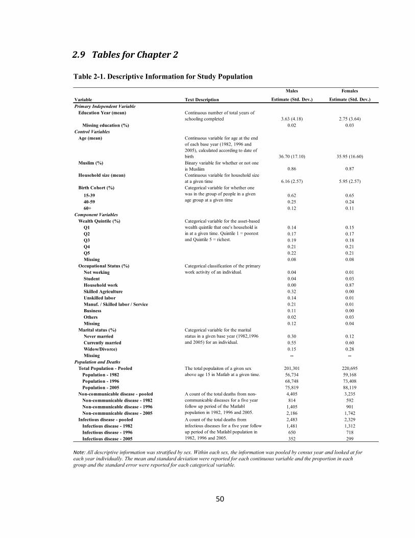
50
2.9 Tables for Chapter 2
Table 2-1. Descriptive Information for Study Population
Note: All descriptive information was stratified by sex. Within each sex, the information was pooled by census year and looked at for
each year individually. The mean and standard deviation were reported for each continuous variable and the proportion in each
group and the standard error were reported for each categorical variable.
Males Females
Estimate (Std. Dev.) Estimate (Std. Dev.)
Primary Independent Variable
Education Year (mean) Continuous number of total years of
schooling completed 3.63 (4.18) 2.75 (3.64)
Missing education (%) 0.02 0.03
Control Variables
Age (mean) Continuous variable for age at the end
of each base year (1982, 1996 and
2005), calculated according to date of
birth 36.70 (17.10) 35.95 (16.60)
Muslim (%) Binary variable for whether or not one
is Musliim 0.86 0.87
Household size (mean) Continuous variable for household size
at a given time 6.16 (2.57) 5.95 (2.57)
Birth Cohort (%)
15-39 0.62 0.65
40-59 0.25 0.24
60+ 0.12 0.11
Component Variables
Wealth Quintile (%)
Q1 0.14 0.15
Q2 0.17 0.17
Q3 0.19 0.18
Q4 0.21 0.21
Q5 0.22 0.21
Missing 0.08 0.08
Occupational Status (%)
Not working 0.04 0.01
Student 0.04 0.03
Household work 0.00 0.87
Skilled Agriculture 0.32 0.00
Unskilled labor 0.14 0.01
Manuf. / Skilled labor / Service 0.21 0.01
Business 0.11 0.00
Others 0.02 0.03
Missing 0.12 0.04
Marital status (%)
Never married 0.30 0.12
Currently married 0.55 0.60
Widow/Divorce) 0.15 0.28
Missing -- --
Population and Deaths
Total Population - Pooled 201,301 220,695
Population - 1982 56,734 59,168
Population - 1996 68,748 73,408
Population - 2005 75,819 88,119
Non-communicable disease - pooled 4,405 3,235
Non-communicable disease - 1982 814 592
Non-communicable disease - 1996 1,405 901
Non-communicable disease - 2005 2,186 1,742
Infectious disease - pooled 2,483 2,329
Infectious disease - 1982 1,481 1,312
Infectious disease - 1996 650 718
Infectious disease - 2005 352 299
Variable Text Description
Categorical variable for whether one
was in the group of people in a given
age group at a given time
A count of the total deaths from
infectious diseases for a five year follow
up period of the Matlabl population in
1982, 1996 and 2005.
Categorical variable for the asset-based
wealth quintile that one's household is
in at a given time. Quintile 1 = poorest
and Quintile 5 = richest.
Categorical classification of the primary
work activity of an individual.
Categorical variable for the marital
status in a given base year (1982,1996
and 2005) for an individual.
The total populaiton of a given sex
above age 15 in Matlab at a given time.
A count of the total deaths from non-
communicable diseases for a five year
follow up period of the Matlabl
population in 1982, 1996 and 2005.
Excludes deaths from Injuries.

51
Table 2-2. OLS Regressions on the components of Wealth, Marital Status and Occupation
Note: Significance: ***p < 0.01, **p < 0.05, *p < 0.1. Data here is pooled for all three time periods. All equations run with the ordinary least squares model: 𝑍𝑖 =𝛽0 + 𝛼𝐸𝑑𝑢𝑖+ 𝛽𝑘𝑋𝑘 + 𝜖𝑖 with controls for age, religion, household size, birth cohort and census year. Wealth is measured by the quintile from 1 to 5. Marital status is coded as binary for either being in the married or unmarried category (single/divorced/widowed). Occupation is coded as binary for being employed or not. Having an occupation of housework is considered the same as no occupation. Detailed models shown in Appendix Table C-1.
Table 2-3. Cox Proportional Hazards Regression for the Education Gradient in Mortality in Matlab, Bangladesh
Note: Significance: ***p < 0.01, **p < 0.05, *p < 0.1. Data here is pooled for all three time periods. All equations run with the cox proportional hazards model: 𝑙𝑜𝑔 ℎ𝑖(𝑡) = 𝛼(𝑡) + 𝛽1𝐸𝑑𝑢𝑖 + 𝛽2𝑋𝑖 with exogenous controls for age, religion, household size, birth cohort and census year. Detailed models shown in Appendix C-2 to C-55
Wealth Occupation Marital status Wealth Occupation Marital status
Coeff on Education 0.11*** 0.01*** 0.01*** 0.15*** 0.02*** 0.01***
Standard Error 0.00 0.00 0.00 0.00 0.00 0.00
R2
0.20 0.05 0.18 0.22 0.04 0.18
N 186,264 186,264 186,264 203,266 203,266 203,266
ParameterMale Female
Male Female Male Female
Hazard Ratio 0.98*** 0.93*** 0.92*** 0.88***
Confidence Interval (0.97-0.99) (0.91-0.95) (0.91-0.94) (0.85-0.91)
R2
0.053 0.041 0.035 0.030
N 186,264 203,266 186,264 203,266
Infectious DiseaseParameter
NCD

52
Table 2-4. Explanatory contribution of components to the education gradient in
NCD or infectious disease mortality in females
Note: Significance: ***p < 0.01, **p < 0.05, *p < 0.1. Data here is pooled for all three time periods. All
equations run with the cox proportional hazards model: 𝑙𝑜𝑔 ℎ𝑖(𝑡) = 𝛼(𝑡) + 𝛽1𝐸𝑑𝑢𝑖 + 𝛽2𝑋𝑖 + 𝛽3𝑍𝑖
where Zi represents either wealth, occupation or marital status. All models include exogenous controls for
age, religion, household size, birth cohort and census year. The % of the Gradient explained is calculated
with the formula: [(𝛽1𝑀𝑜𝑑𝑒𝑙 1 − 𝛽1
𝑀𝑜𝑑𝑒𝑙 2)/𝛽1𝑀𝑜𝑑𝑒𝑙 1] ∗ 100], where model 1 is the base model and model 2 is
the subsequent models with the individual component added or with all three added together. Detailed models shown in Appendix C-4 and C-5.
Model Parameter NCD % Gradient Infectious Disease % Gradient
Hazard Ratio 0.93*** -- 0.88*** --
Confidence Interval (0.914-0.954) (0.851-0.910)
R2
0.041 0.030
N 203266 203266
Hazard Ratio 0.94*** 14% 0.89*** 11%
Confidence Interval (0.923-0.963) (0.863-0.922)
R2 0.041 0.030
N 203266 203266
Hazard Ratio 0.93*** 1% 0.88*** NA
Confidence Interval (0.914-0.955) (0.850-0.909)
R2 0.041 0.031
N 203266 203266
Hazard Ratio 0.97*** 52% 0.90*** 16%
Confidence Interval (0.947-0.989) (0.868-0.928)
R2 0.051 0.035
N 203266 203266
Hazard Ratio 0.97*** 59% 0.91*** 27%
Confidence Interval (0.950-0.995) (0.881-0.941)
R2
0.051 0.036
N 203266 203266
Add Wealth +
Occupation +
Marital Status
Base Model
Add Wealth
Add Occupation
Add Marital Status

53
Table 2-5. Explanatory contribution of the components to the education gradient in
NCD or infectious disease mortality in males
Note: Significance: ***p < 0.01, **p < 0.05, *p < 0.1. Data here is pooled for all three time periods. All
equations run with the cox proportional hazards model: 𝑙𝑜𝑔 ℎ𝑖(𝑡) = 𝛼(𝑡) + 𝛽1𝐸𝑑𝑢𝑖 + 𝛽2𝑋𝑖 + 𝛽3𝑍𝑖
where Zi represents either wealth, occupation or marital status. All models include exogenous controls for
age, religion, household size, birth cohort and census year. The % of the Gradient explained is calculated
with the formula: [(𝛽1𝑀𝑜𝑑𝑒𝑙 1 − 𝛽1
𝑀𝑜𝑑𝑒𝑙 2)/𝛽1𝑀𝑜𝑑𝑒𝑙 1] ∗ 100], where model 1 is the base model and model 2 is
the subsequent models with the individual component added or with all three added together. Detailed models shown in Appendix C-2 and C-3.
Model Parameter NCD % Gradient Infectious Disease % Gradient
Hazard Ratio 0.98*** -- 0.92*** --
Confidence Interval (0.972-0.987) (0.911-0.936)
R2
0.053 0.035
N 186264 186264
Hazard Ratio 0.99*** 48% 0.94*** 20%
Confidence Interval (0.979-0.999) (0.925-0.951)
R2
0.053 0.035
N 186264 186264
Hazard Ratio 0.98*** 19% 0.94*** 21%
Confidence Interval (0.974-0.993) (0.923-0.949)
R2 0.053 0.035
N 186264 186264
Hazard Ratio 1.00 NA 0.94*** 21%
Confidence Interval (0.995-1.011) (0.926-0.952)
R2 0.107 0.049
N 186264 186264
Hazard Ratio 1.00 NA 0.96*** 49%
Confidence Interval (0.985-1.024) (0.947-0.973)
R2
0.107 0.050
N 186264 186264
Add Wealth +
Occupation +
Marital Status
Base Model
Add Wealth
Add Occupation
Add Marital Status

54
2.10 Figures for Chapter 2
Figure 2-1. GDP per Capita (US$) for Bangladesh
Note: GDP – Gross Domestic Product per capita, measured in US$ using current prices.
Reference: IMF World Economic Outlook (47).
Figure 2-2. Percentage of the Population of Bangladesh in Poverty
Note: 1992 is the earliest year for which poverty headcount estimates are available. % Rural poverty is
equal to the poverty headcount ratio at the rural poverty line (% of rural population). % National Poverty
is equal to the poverty headcount ratio at the national poverty line (% of population). Reference: World
Bank Poverty and Inequality Database (48).
0
50
100
150
200
250
300
350
400
450
1982 1985 1988 1991 1994 1997 2000 2003 2006
GD
P p
er c
apit
a
Year
0
10
20
30
40
50
60
70
1992 1994 1996 1998 2000 2002 2004 2006
Po
vert
y h
ead
cou
nt
(%)
Axis Title
% Rural Poverty
% National Poverty

55
Figure 2-3. Mean Years of Education Completed by Sex in Matlab, Bangladesh
Note: Observations are the mean of the continuous year of education for males and females at three time
points: 1982, 1996 and 2005.
Figure 2-4. Mortality from Non-communicable and Infectious Diseases in Matlab,
Bangladesh
Note: Mortality hazard calculated as the number of deaths from a given cause (NCD or infectious divided
by the total person years contributed over the 5-year follow up for each of the timepoints 1982, 1996 and
2005.
0
0.5
1
1.5
2
2.5
3
3.5
4
1980 1985 1990 1995 2000 2005
Mea
n y
ear
of
edu
cati
on
co
mp
lete
d
Year
Male
Female
0.000
0.001
0.002
0.003
0.004
0.005
0.006
0.007
1980 1985 1990 1995 2000 2005 2010
Mo
rtal
ity
Haz
ard
Year
NCD
INF

56
Figure 2-5. Non-communicable Disease Mortality by Education for Matlab,
Bangladesh
Note: High education is more than 5 years completed and low education is 5 or less years of education
completed.
Figure 2-6. Infectious Disease Mortality by Education for Matlab, Bangladesh
Note: High education is more than 5 years completed and low education is 5 or less years of education
completed.
0
0.005
0.01
0.015
0.02
0.025
1980 1985 1990 1995 2000 2005 2010
Haz
ard
of
Mo
rtal
ity
Year
NCD - HIGH
NCD - LOW
0
0.005
0.01
0.015
0.02
0.025
0.03
0.035
1980 1985 1990 1995 2000 2005 2010
Haz
ard
of
Mo
rtal
ity
Year
INF - HIGH
INF - LOW
57
Chapter 3. The Household Economic Impact of a Non-Communicable Disease Death in Matlab, Bangladesh: An Empirical Application of Regression Standardization
3.1 Abstract
Adverse health events may negatively impact the economic condition of a household. In
low and middle-income countries with a growing portion of their disease burdens coming
from non-communicable diseases (NCD), the consequences of poor health from NCDs
have not been fully explored. This work evaluates the risk of being poor for households
with an adult NCD death. A cohort study is conducted in a rural area of Bangladesh, and
a marginal estimator using regression standardization, is used to estimate the economic
impacts of a death. Three different measures of economic outcomes are explored: an
asset-based index, self-rated household economic condition and total household
landholding. The results show that households with an adult NCD death had a
significantly higher marginal risk of being poor up to two years after the death that
ranged from 14-19%. This effect was significant for all three outcomes of economic
condition. Comparing the regression standardized results to those using traditional
contingency tables and multivariate regression found similar results. The regression also
showed that a death to a prime, working-age (ages 15-59) household member leads to a
significantly higher risk of being poor when using an asset index or self-rated economic
condition. This work emphasizes the need for more intense prevention efforts for NCDs
and for better financial protection from health shocks in rural Bangladesh. The finding of
a significant economic impact for households experiencing NCD deaths means that
programs to address the burden of NCDs and policies that provide for better access to
care and risk-pooling for households will aid the economic development in rural

58
Bangladesh. Future work should disentangle further the mechanisms through which
economic impacts from an NCD death shock occur.
3.2 Introduction
There is a strong positive association between health and wealth. This relationship was
made explicit at a country level with the work of Samuel Preston in 1975 who looked at
the relationship between life expectancy and per capita gross domestic product (GDP)
(Preston 1975). At the microeconomic level there are attempts to understand the health
and wealth relationship as bi-directional. In the direction of wealth to health, research has
focused on the effect of more economic resources leading to better health outcomes.
Alternatively, economic research to understand the relationship in the opposite direction,
from health to wealth, establishes a framework for wealth impacts through increased
health expenditure, changes to labor participation, changes to human capital and changes
in the marginal utility of consumption (40).
One approach for assessing the effects of health on wealth at the micro level has been to
look at “health shocks”, defined as an unanticipated event that leads to economic losses
and constrained opportunities for households (21, 96). Health shocks, when assumed to
be exogenous, have also been used as tools for economists for solving the endogeneity
problem between health and wealth. For a shock from a death to a household member,
increased health expenditures and losses of human capital are detrimental to a
household’s overall economic condition (97). In low and middle-income countries this
may be especially true since there is limited access to social protection and risk-pooling
mechanisms (98). In terms of shocks from adult mortality, the economic impacts have
59
been looked at for communicable diseases such as HIV/AIDS and found that there are
significant costs to individuals and households in terms of reduced consumption and
human capital (97, 99). Others have found economic impacts on children when there is an
adult death (100). There have also been studies that look at non-mortality health shocks
such as self-reported morbidity and the associated economic impacts (101). Overall, the
evidence supports that health shocks have a negative economic impact on households
through increased medical expenditure and reduced human capital. In contrast, in some
settings, there have also been studies showing no effects or even improved economic
outcomes after health shocks, showing the complexity of the issue. The impact of health
shocks from NCD mortality have not been studied as well but there is evidence that they
have the potential to be even more severe than those from other causes of disease (20).
NCDs are also predicted to play a role in the understanding of socioeconomic mobility
and poverty traps. Recent research has examined NCD-related poverty issues in low-
income countries and found that there are important interactions with NCDs and poverty
(102, 103).
NCDs are a growing portion of the disease burden in low and middle-income countries
and particularly troubling is the premature mortality from NCDs. A 2010 report by the
World Health Organization (WHO) found that 29% of NCD deaths were in people
younger than 60 years old in low and middle-income countries, whereas this same
statistic was 13% for high income countries (11). In Bangladesh, non-communicable
diseases (NCD) represent the leading cause of mortality and there has been a large
growth in the proportion of deaths from NCDs over time (3). In the rural area of Matlab,
Bangladesh, a demographic surveillance site with ongoing cause of death monitoring,

60
there have been age-adjusted increases in the mortality rates from NCD specific causes
(5).
Examining the economic impact to households from NCD deaths may be an issue given
the bi-directional relationship between health and wealth. For this reason, NCD health
shocks in terms of adult mortality are used in a matched cohort study design in the
Matlab demographic surveillance area. An extension of standardization methods, using a
regression standardization approach, was developed recently for matched cohort analysis
is used to provide a marginal effect (104). The regression standardization method is
implemented with a parametric model and with a machine learning function to address
the well-known limitations of parametric models. More specifically, the major limitation
of parametric models is the assumption made about the underlying data distribution. In
practice it is very unlikely that one can correctly specify the functional form of the
parametric regression. These concerns have been discussed widely in the statistics and
epidemiology literature (105-108). This approach of combining machine learning and
effect estimation has been shown to be more robust to model misspecification than
traditional, parametric approaches (108). Here, this approach is used to provide a policy-
relevant estimate, a marginal estimate of the effect among the exposed, for mitigating the
risk of poverty for those experiencing adult NCD health shocks.
The objective of this study is to evaluate whether households in rural Bangladesh
experiencing mortality shocks from NCDs have a higher risk of being poor two years
after death. This is done with the use of a regression standardized marginal estimator and
a novel machine learning standardized estimator in Matlab, Bangladesh, a rural area with

61
demographic surveillance. These results are compared with traditional analyses
approaches using contingency tables and multivariate regression. As a sub-objective the
economic impacts from NCD death are evaluated for whether they differ by individual
characteristics such as prime age (working age) status, sex, marital status and position in
the household.
3.3 Literature Review
3.3.1 The Economic Consequences of Poor Health
In aggregate, the positive relationship between health and wealth shows that countries
with a lower GDP have worse health, in terms of life expectancy, and that higher national
income is related to better life expectancy (7). The existence of a positive relationship
leads to a question of the directionality of the relationship between health and wealth. At
the aggregate level, there have been attempts to look at the effect of increasing income on
health, and also the reverse effect, how better health leads to more wealth or income.
There have also been attempts to explore this relationship at the micro level of the
individual and the household. In low income countries, shocks from health events have
been reported to be an important for the economic situation of the household (21). These
micro-level economic impacts were explored by Gertler and Gruber who found that
households in Indonesia may not be able to fully smooth consumption (adjust for
economic losses) after health shocks (20).
There are two frameworks that have been used to look at the economic impacts from
health shocks (42, 43). Such mortality shocks result in the loss of human capital for

62
households and may result in the loss of income earning potential as well. Often, the most
devastating impacts of mortality shocks have been to households experiencing deaths of
prime working-age adult members (97, 109).
Other studies in developing countries that have looked at the impact of adult health
shocks have been in settings of high HIV/AIDs prevalence. This work has taken place in
with datasets from Tanzania, Kenya, Mozambique and Zambia and are primarily
concerned with death from adult, economically productive household members (97, 99,
109-111). These studies find differences in the effects on households from prime-age
mortality based on the age and gender composition of the households, the initial wealth
and the labor and agricultural characteristics of the community. Outside of the HIV/AIDS
literature, other analyses have been conducted looking at the impacts of health shocks on
household wealth outcomes in low income country settings (112, 113).
The importance of understanding the effects of prime age, or economically active, adults
depends on whether the person that died was a net consumer or net producer for the
household. It also depends on whether the earning activities of the household are
changed, called income coping, and whether the composition structure of the household
is changed, called demographic coping (109, 111). The issue of coping is examined in the
next framework.
3.3.2 Economic Consequences of Non-communicable disease
The growing burden from NCDs has the potential to have large economic consequences.
Recent work estimates the global output loss from NCDs such as CVD, chronic

63
respiratory disease, cancer, diabetes and mental health be near $47 trillion (8). At the
microeconomic level, other studies have shown households experiencing NCDs may
have worse economic outcomes than those with poor health from communicable diseases.
This was seen in the data originally with self-reported health (20). Analyses have also
shown that households with chronic illness, ex post, are more likely to be in the lower
two socioeconomic quintiles (lower 40% of the wealth distribution) (114).
At the household level, the economic impact from an NCD may be realized through
higher out of pocket expenditures (OOP). This has been seen in research in Russia and
Ukraine where there are formalized systems for financial risk pooling (115, 116). One
study in South Asia found a similar result, with larger OOP health expenditure in for
households with angina in India (96).
Another explanation for the economic impact from NCDs comes from the effect on labor
supply. In studies looking at health shocks from illness episodes, not deaths, the effect on
labor income was found to be a reduction of nearly 5% for NCD illness with no
significant loss for households with a communicable disease illness (115). In terms of
labor participation, two studies in South Asia have found that household labor decreases
overall by about 2-3% compared to a control group when there is an NCD (117, 118).
The reduced labor participation is also seen in studies of the impact of a death, which
reduces labor participation through the reduction of human capital of a household (99).
When examining labor participation, however, there is also a possibility that the non-sick
members of the household will increase labor participation and earn more income to cope
with the health event or death.

64
While OOP medical expenditure and labor outcome have been found to be worse for
households with NCDs, another measure of general economic impact is non-medical
expenditure. For this outcome, studies that have looked at NCDs have found more mixed
results (96). While one study in India found a small decline in non-medical expenditure
for households with heart disease, another study looking at angina in multiple South
Asian countries did not find any reduction in non-medical expenditure (96, 117). One
explanation for this may be that NCD health events take place in older age groups where
households have time to adjust finances and can even anticipate the onset of a death. In
these settings, some households, from an economic standpoint, may even be better off
following a death of an older household member that is a net-consumer.
3.3.3 Accounting for Endogeneity between Health and Wealth
Understanding the relationship of NCD deaths with household economic condition in
Bangladesh presents some methodological challenges. The endogenous relationship
between health and wealth means that cross-sectional associations will not provide a
causal indication of the level of economic impact that could be realized that would come
from a reduction of the NCD burden. Shocks are usually considered to be idiosyncratic
and exogenous, and because of these properties, could provide some conclusion about the
causal relationship between health and wealth (119). A recent review, has shown that
when measuring the effects of health shocks, there is a heterogeneity of methodologies to
account for endogeneity, economic outcomes used and types of health events used (96).
Some studies have constructed a counterfactual comparison group with matching through
direct matching approaches and through propensity score matching approaches to account
for the endogeneity between health and wealth (116, 118). These approaches, as well as

65
implementation of fixed effects in regression help account for time invariant
unobservable factors that may confound the results. Further work has also used
instrumental variables estimation, which also accounts for time variant unobservable
effects, but which may pose more burden on the researcher to identify a valid instrument
(115).
This study does not make final causal conclusions about the impact of health on wealth
because there may be other unobservable confounders that are not identified here. This
study does however use an epidemiologic study design, a matched cohort study, and a
novel estimator to account for all of the measured confounding and to provide a marginal
estimate. There is also a chance that the addition of an instrumental variable estimation
approach to address unobserved confounding would change these results, which would
further strengthen any causal conclusions. This study is one of the first in the health
economics literature to use a matched cohort design and regression standardization to
obtain a marginal effect in combination with a super learner machine learning algorithm.
There have been other examples of these approaches in the biostatistics and epidemiology
literature (104, 120).
3.4 Data
The data for this study come from two different sources. One is the ongoing health and
demographic surveillance conducted by the International Center for Diarrhoeal Disease
Research in Bangladesh (icddr,b). This surveillance is a yearly census of all vital events
for the Matlab population. As a part of this surveillance, there is a periodic

66
socioeconomic status census, approximately every ten years, which collects information
on the ownership of household assets.
A strength of using this surveillance data is the ability to select households with NCD
deaths from administrative census data. Having census data for deaths that includes cause
of death information means we can identify all households that had NCD deaths in 2010.
This is a unique situation for a rural, poor population in a developing country. Other
surveys of health-related impact suffer from endogeneity bias due to self-rated shocks
where upward bias is possible if a household member is more likely to remember a shock
because it is severe (112). In addition to collecting information on deaths, data for
specific causes of death by ICD-10 coding allows for accurate identification of the causes
of death. Previous studies in low-resource settings where cause of death information is
not available have had to use proxy variables such as age of death to determine the cause
(111).
Using mortality as the primary independent variable provides an objective measure,
subject to less bias than a subjective health rating. Using self-rated health may be
insufficient if notions of well-being differ systematically in different cultures. For this
reason, self- assessed functional status or objective health measures are found to be better
(121).
The second source of data for this study is a survey that was designed to evaluate the
household economic impact of NCD mortality. This survey was collected for the study
population in Matlab in the year 2012 and is found in the Appendix 7.1. Separate
modules in the survey collected information on the socioeconomic and demographic

67
characteristic of the household, information about the NCD death in 2010 and subsequent
household coping strategies.
The study population consists of all adult deaths, defined as 15 years or older, from
NCDs that were recorded in the routine surveillance for Matlab in the calendar year 2010.
Using a lower age of 15 is justified for a rural, low income setting such as Matlab where
most people complete education and enter the work force by this age (56). There were
909 adult NCD deaths in Matlab in 2010 identified by routine surveillance. Of these 909,
856 of the households were surveyed in 2012, meaning that there was a 6% attrition rate
for the study. The group of households where these deaths occurred is referred to as the
“NCD group” for the remainder of this study.
Each individual in the NCD group was matched to another individual in a household with
no deaths in the year 2010. The group of households with this individual is referred to as
the “comparison group”. The direct matching procedure was based on the age, sex and
village of the deceased individual. Deceased individuals and comparison individuals were
matched exactly on sex and within 5 years on age. Comparison individuals residing in the
same or nearest village meeting these criteria were selected. Three matching households
were identified for each individual in the NCD group, of which, up to two were
interviewed. A diagram showing the study design is shown in Figure 3-1.
3.4.1 Primary Dependent Variables for Economic Impact
This study used three measures of economic status: an asset-based wealth index, self-
reported economic condition and the total amount of land that a household owns. These

68
were collected in the 2012 survey. Each of these measures was assessed in 2012, when
the interview was conducted for both of the groups. Table 3-1 provides a definition for
each one of these outcomes.
The three different measures provide a picture of the economic status of the households
from different lenses. The asset-based index using durable household items has been used
in Matlab for decades and provides a validated estimate for the distribution of wealth
based on these items. The latent wealth variable, however, may also be captured with the
self-rated economic condition measure, which takes into account non-asset components
of wealth and subjective perceptions of wealth as well. Further testing is done with a
measurement of total landholding, which is common for areas of rural Bangladesh such
as Matlab with an agrarian economy. This measure, however, also suffers from
limitations when there shifting importance of agriculture in the economy. A matrix of
pros and cons for each measure is listed in Figure 3-2.
3.4.1.1 Asset-based wealth index
An asset index was calculated as a measure for wealth, which is typically done in the
absence of data on income or consumption (88). The index was calculated with a
principal component analysis (PCA) of 26 durable household goods collected in the
survey in 2012. PCA is a common method for transforming a list of assets into an index
that measures wealth when information for prices is not available. PCA, however,
provides a cross-sectional snapshot of the economic condition of an area and may not be
ideal when understanding longitudinal changes in socioeconomic status is needed (122).

69
The cross-sectional nature of PCA presents problems for looking at asset scores over
multiple time periods. When PCA weights (the eigenvalues derived from PCA) are used
for more than one time period, the weights can be applied either to the pooled sample or
to the baseline sample with an assumption that the relationship between asset ownership
and wealth is constant (123). Following this suggestion, for our study, one option would
be to use the PCA weights from the 2005 socioeconomic status surveillance census to the
survey data from 2012. Another suggested solution to this issue is to use a modified
version of PCA called polychoric principal component analysis (PPCA) that has been
proposed as a better approach to measure asset-based wealth over multiple time periods
(122). PPCA better accounts for differences across time because it provides a weight for
asset ownership as well as non-ownership with a negatively signed weight.
PPCA was run for the list of assets collected in Matlab in 2005 and the weights were
applied to the same listing of assets which was collected for the 2012 NCD economics
survey. Being poor was defined as being in the bottom 40% of the wealth distribution,
which is the lowest two wealth quintiles.
The limitations of asset-based wealth measurement have been well-documented. A
primary limitation for this measurement is that a lack of prices prohibits assigning a
monetary value to the assets. The quality and length of time that the household has held
the assets are also not measured. Studies on the relationship of asset indices with detailed
surveys of consumption in India have found poor correlation (124).

70
3.4.1.2 Self-rated economic condition
The second measure of economic condition was household self-rated economic condition
according to a 5-step subjective ladder. These types of subjective ladders of
socioeconomic status have been called Macarthur scales and have been used as
alternatives to objective socioeconomic status measures or when understanding perceived
economic status. Similar self-rating scales have been used in prior work looking at the
economic impact from health shocks in low income country settings (112) (21, 125).
The survey asked surviving respondents to assess the household economic condition in
2012 at the time of the interview, approximately two years after the NCD death.
Household representatives were asked to mark their economic condition onto a 5-step
ladder with steps representing: 1 – very poor, 2 – poor, 3 – not poor or rich, 4 – rich and 5
– very rich. (126). When identifying interview respondents, measures were taken to
ensure that individual could speak about the general economic condition of the
household.
Households that marked that they were in the first two rungs of the ladder were
considered poor. An example of the survey question for self-rated economic condition is
shown in the full questionnaire in the Appendix 7-1.
For self-rated economic outcome, there may be bias resulting from using recall data from
up to two years in the past. The households could either forget about the significance of a
death or exaggerate the impacts as being too severe. Attempts to minimize this bias for

71
this study came from constructing disease timelines and using natural events (e.g. the
annual wet season) as reference points.
3.4.1.3 Landholding
The third measure of economic condition is a measure of total household landholding.
This comprised both residential land and agricultural land. The use of landholding as an
indicator of wealth status has been used previously in rural areas that have a high level of
agricultural activity. This study used a threshold of 50 decimals (dm) of landholding to
determine poor status. A decimal is a measure of land area that is only used in certain
parts of India and Bangladesh. It is equal to 1/100 acre or 40.46m2. Previous work in
rural Bangladesh has validated this threshold as an indicator of poverty (127).
A limitation of using the measurement for landholding as a measurement for wealth is
that it only captures wealth through this single dimension. With the growth of businesses
and increasing education in the rural areas of Bangladesh, opportunities for non-
agricultural income generation are likely becoming more prevalent. Further, there is no
indication of the quality of the land that is owned or income generated from external
sources such as remittances or safety net transfers. Households may also be incentivized
to underreport landholdings if they think that sharing that information would lead to
higher taxation. Regardless of these limitations, there is indication that land is still a
central component of a household’s assets in rural Bangladesh and that owning no land
may be a good indicator of destitution.

72
3.4.1.4 Relation between the three economic outcomes
An overall description of the pros and cons of each of the economic outcomes is provided
in Figure 3-2. Descriptive information is shown for the three economic outcomes of
interest in Table 3-1. At the time that the survey was administered in 2012, the
percentage of the population classified as poor differed depending on which measure is
used. Using the asset index, 22% of the study population was classified as poor in at
follow up. This is 42% when the self-rated economic condition and 63% according to the
threshold of owning 50dm of total land. The correlation between the different measures is
also shown in Table 3-1. The largest correlation is between the asset index and the self-
rated condition, which has a Spearman rank coefficient of 0.39. The asset index and total
landholding show the lowest amount of correlation, with a coefficient of 0.26. Comparing
the correlation of self-rated economic condition and landholding also shows low amounts
of correlation, with a Spearman coefficient of 0.32.
3.4.2 Primary Independent Variable – Non-Communicable Disease
Mortality
The 909 adult deaths from NCDs were identified by International Classification of
Disease version 10 (ICD-10) codes that are assigned by the surveillance team in Matlab
through a dual physician review verbal autopsy. Deaths from injuries including
unintentional injury such as accident and drowning, and intentional injury such as suicide
and homicide were excluded (128). The final NCD deaths included deaths from: cancer,
COPD, diabetes, cardiovascular disease (including hypertensive disorders, ischemic heart
disease and stroke), blood disorders, metabolic disease, mental disorders, neurological

73
disease as well as other respiratory and digestive diseases. An illustration of the total
numbers of deaths in each category is shown in Figure 3-3.
3.4.3 Further Independent Variables
The covariates used for stratification and in the multivariate analysis were collected
through the routine surveillance for Matlab. These were obtained from the demographic
surveillance system for the year 2009, the year prior to the NCD death. For the deceased
individual, data were obtained for age, sex, household position, marital status and
education. Data were also obtained for household-level characteristics such as religion
and household size. The variable for household size may be an indicator of the total
resources available to the household (129). All of the independent variables are assumed
to be exogenous to the relationship of an NCD death on a household’s economic
condition.
Descriptive statistics for the independent variables are seen in Table 3-2. The distribution
of variables that were used for matching: age, sex and village show that there is balance
among the groups. The mean age is around 68 years and 21% of each group is considered
prime age. Additionally, 45% of each group is female and the individuals in the NCD
group also come from 135 different villages while those from the comparison group
come from 145 villages.
The other individual-level variables show that a large proportion of the study population
has no education and about a quarter have completed some primary education, up to 5
years of formal schooling. Only 15% has completed more than 6 years of formal

74
schooling. For marital status, 62% of the study population is married and 36% are
widowed. A small percentage report being either unmarried or divorced, 2% and 1%
respectively.
Position within the household was measured as a binary variable for whether one was the
household head or spouse of the household head. This is the only independent variable
which shows a significant difference between groups. 67% of the NCD group and 73% of
the comparison group are either household heads or spouses of the household head. The
percentage of households self-reporting their economic condition as poor prior to the
death is also shown. Here, 44% of the NCD households and 43% of the comparison
households self-report as poor either before the death in the former or in 2009 for the
latter. By this measure, the households do not appear to be different in economic status at
baseline.
Household-level independent variables were included for total household size and
religion. These did not differ between groups. The mean household size was around 6.2
persons and 86% of the population was Muslim.
3.5 Analytical Framework
3.5.1 Study Design
This study uses a matched cohort design with exposure-driven sampling, the exposure of
interest being an adult death from an NCD (130). Matched cohort designs are relatively
rare compared to other designs, but it is used here because of the availability of
75
surveillance information for all households in Matlab and the ability to identify all deaths
for a given time period by cause. The matching procedure establishes a comparison group
that potentially balances confounding variables related to the household’s economic
status at baseline (131). Using a matched cohort design also means that adjustment can be
done for the variables used for matching. The longitudinal nature of the cohort design
also means that household and individual characteristics are removed that could affect the
economic impact of an NCD death (131).
The differences between descriptive characteristics for the NCD group and the
comparison group at baseline are first assessed. There is ambiguity in the literature about
whether accounting for matched variables in a matched cohort analysis is needed. We use
a t-test statistic for continuous variables and assuming independence between the groups.
A paired t-test may also be used in matched cohort study, and we find similar result when
using a paired or unpaired test but only report the unpaired results (104, 132). A chi
squared test for independence is used for categorical variables (133).
3.5.2 Method 1: Marginal Effect Estimation with Regression Standardization and Machine Learning
The strategy uses an estimator of marginal effect calculated through regression
standardization, an extension of traditional standardization methods (104, 134). This
estimator uses the marginal distribution of the baseline covariates and matching variables
in the exposed subjects to estimate the familiar average exposure effect on the exposed
parameter. This parameter is most commonly referred to as the average treatment effect
on the treated (ATT) in the health economics and statistics literature when a treatment is

76
of interest instead of an exposure (135-137). Inverse probability weighted methods have
also been used to estimate marginal parameters, however, these estimators can have poor
performance in practice with respect to bias and efficiency, particularly when the
probability of exposure is large or small. The standardized estimator is calculated through
a process of marginalizing over observed covariate distributions in the exposed subjects
after obtaining counterfactual outcomes, given that all possible exposure scenarios are
unobserved. This is because the creation of a true counterfactual scenario, which is the
goal of causal inference, is never observed with empirical data. The parametric versions
of the estimator use regression functions based on an a priori specified parametric model
to calculate the expected counterfactual scenarios and obtain a marginal effect (104, 120).
The steps for regression standardization are as follows:
1. Estimate the outcome regression using the traditional parametric approach:
𝐸(𝑌|𝐴, 𝑊). The expected value of the outcome Y given the exposure to an adult
NCD death A, conditional on all of the covariates of interest, W. The vector W
also contains the matching variables.
2. Use the equation in step 1, to obtain each observation’s predicted value under the
condition that they were exposed to an adult NCD death (A = 1).
3. Repeat step 2, except this time obtain the predicted values with each observation
not being exposed to an adult NCD death (A = 0).
4. The predicted values from steps 2 and 3 are then used to calculate the estimator of
interest:
�̂�𝑅𝑅 =1
𝑁∑ [�̂�(𝑌|𝐴=1,𝑊)]𝑁
𝑖=11
𝑁∑ [�̂�(𝑌|𝐴=0,𝑊)]𝑁
𝑖=1
,

77
which here estimates the relative risk parameter of exposure among the exposed.
5. Use bootstrapping to obtain standard errors for the marginal effect of interest
obtained from step 4.
One of the limitations of this approach regards fitting the model in step 1. If this model is
misspecified, then bias could result in the standardized estimate as well. To explore this
further, a machine learning algorithm is used for specifying the regression function and
calculating a subsequent standardized estimator. Machine learning is a broad term for
flexible computational techniques that use the data to “learn” in order make estimations,
generalizations or predictions (138). Machine learning can be used to estimate the
conditional expectation given baseline covariates with a more versatile bias-variance
trade-off. These methods have been used widely for purposes of prediction and
classification; however, more recently, machine learning has been incorporated into
effect estimation. When machine learning is integrating into the estimation process for
effects, cross-validation must also be implemented to evaluate over-fitting. Cross-
validation is the process of dividing a dataset into separate smaller datasets for validation
purposes (also referred to as “hold-out samples.”) Overfitting is assessed in this fashion
by the ability of the algorithm to predict values out of the sample of interest (105, 107,
108, 138).
The machine learning algorithm that is implemented here is a “super-learner”, which is
an ensembling machine-learning approach (107, 108). Super learning is a framework that
allows for the use of multiple machine learning algorithms while producing the best

78
weighted average of these candidate learners. This is implemented in step 1 of the above
5 step process. The application of the super-learner machine learning algorithm for a
matched cohort design is described in full detail in a companion paper to this work (139).
The super learner algorithm is implemented in R programming language using the
SuperLearner package (140). A collection of 3 algorithms were used in this analysis:
logistic regression implemented with the generalized linear models (glm) package, the
arithmetic mean where the marginal probability of being poor in each cross-validation
fold is assigned to each household and a final package (glmnet) for penalized regression
using the least absolute shrinkage and selection operator (LASSO) (141). Super learner
performs cross-validation internally, such that the optimal final weighted average of
algorithms is built based on algorithm performance in the “hold-out” samples.
Bootstrapping is used for obtaining standard errors and confidence intervals.
3.5.3 Method 2: Contingency Tables Analysis
Contingency tables are a traditional method for examining epidemiologic effects.
Following recommendations for a matched cohort study with binary treatment and
outcome variables, a 2x2 contingency table was used to show the relative risk of being
poor two years after death given an NCD mortality shock (132, 142). Stratified
contingency tables were used to adjust for variables used in the direct matching as well as
other independent variables of interest.

79
3.5.4 Method 3: Log-Binomial Regression
Multivariate analyses were conducted with a log-binomial regression model. This model,
which is mathematically similar to the Poisson regression approach, produces estimates
of the relative risk conditional on all independent variables of interest. The model is
specified as follows:
𝑙𝑜𝑔 𝑌𝑖(𝑡) = 𝛼(𝑡) + 𝛽1𝑁𝐶𝐷𝑖 + ⋯ + 𝛽𝑘𝑋𝑖 (1)
Where Yi is an indicator of whether household i is poor or not according to one of the
three measures for economic status. 𝛽1 is the coefficient on the indicator for whether a
household had an NCD adult death in 2010. Taking the exponent 𝛽1 gives the relative risk
of being poor for households with an NCD death. 𝛽k is the coefficient on the other
independent variables of interest, given by the vector Xi. The model is run separately for
each of the three economic outcomes of interest and standard errors are clustered by
household. An interaction terms is used in the regression model to assess if the risk of
poverty following a health shock is different according to the prime-age status of the
individual.
3.6 Results
The results for this matched cohort study are presented with three different methods: a
marginal regression standardization estimator, a traditional contingency table approach
and multivariate log-binomial regression approach. The regression standardization
estimator gives the marginal effect on economic condition following an NCD death

80
accounting for the distributions of NCD deaths in Matlab as well as the other independent
covariates, among those with an NCD death. These are compared to contingency tables
and a log-binomial regression. The regression also examines whether the economic
impact of having an NCD death is modified when the death is to a prime age member of
the household.
3.6.1 Method 1 Results: Regression Standardization for Marginal Effects Results
The results of the regression standardization estimator using parametric regression are
shown in Table 3-3. The results represent the marginal effects for the risk of being poor
in 2012 given an adult NCD death in 2010. Using the asset-based quintile, the relative
risk is 1.19 and significant meaning that having a death leads to a 19% greater risk of
being poor. For self-rated economic status, the results show that there is a significant
relative risk of 1.16, meaning that there is a 16% higher risk of a household perceiving its
status as poor in 2012 after the death in 2010. For the variable of land-holding, the risk of
being poor is also positive and significant and shows a 14% higher risk of a household
being poor given an NCD death (relative risk: 1.14). The results with the super-learner
machine learning approach show similar results to the regression standardization
approach but overall have slightly smaller relative risks. Interestingly, the relative risk
using the asset-based quintile, 1.15, is no longer statistically significant since the
confidence interval crosses one (CI: 0.98 to 1.32). The results for self-rated condition
(RR = 1.13) and land-holding (RR = 1.11), however do find significantly elevated risks
of being poor.

81
The use of a matched cohort for census data and a relative risk approach for assessing the
economic impacts of mortality is novel and these results are not directly comparable to
previous research, however, some relative understanding of these results are needed.
Using cross-sectional data for Matlab in 1982 and 1996, previous researchers have found
that the relative risk of mortality for adults aged 15-59 for a poor versus a non-poor group
was around 1.40 (62). The results from this work then show that the relative risk of being
poor after an adult NCD health shock is somewhat lower. Another paper in Vietnam
assesses the risk of moving into a poor state for those that are non-poor before an injury
and find a relative risk of 1.21. They also find that those who are poor and have an injury
are less likely, by 4% to move out of poverty. Several studies, however, use a self-
reported measure of economic well-being to assess the impact of a health shock. In
Tanzania on study found that 20% of households reported having a year of “very bad”
living conditions specifically due to the death of a household member (129). Another
study in Vietnam found that households with shocks from deaths reported being more
likely to have decreased welfare than did households experiencing shocks from droughts.
When looking at changes in consumption, several studies have also found declines in
consumption following a health shock from mortality. Estimates for the reduction in
consumption have been 7-8% (143, 144). Results for the effect of health shocks on
poverty incidence have also shown that this could be as large as 2% (143).
3.6.2 Method 2 Results: Contingency Tables
The results for the relative risk of being poor following a death from an NCD are shown
with the contingency table calculations in Table 3-4. For the pooled group a significant
risk of being poor after the death is found using the asset quintile. The relative risk of

82
1.19 means that there is a 19% higher risk of being poor two years after an adult NCD
death compared to a comparison household with no death. Stratifying the study
population by the individual characteristics of the deceased, significant increased risks of
being poor according to the asset quintile are also seen for deaths to prime age household
members and married members. The death of a prime age member leads to nearly two
times the risk of being poor, while the death of a married member leads to a 26% higher
risk (relative risks: 1.96 and 1.26).
For the outcome of self-rated economic condition in Table 3-4, the pooled sample shows
a significant increased risk of being poor for those with an NCD death with a relative risk
of 1.14. The stratified samples also show that deaths to male members, prime age
members, uneducated members, married members and household heads lead to
significant increased risks of being poor. The largest increase in risk of death is for a
prime age member, where a death results in nearly a 50% increase in the risk of being
poor (relative risk: 1.49).
The relative risk of being poor according to landholding is also shown in Table 3-4. In
the pooled sample, the relative risk of being poor given an NCD death is 1.10 and is
significant. In the stratified samples, the death of a male member, old age member,
member with primary education, married member or household head show significant
increased risks of being poor. The highest relative risk here is seen with the death of a
member of the household with primary education, which raises the risk of being poor by
30% (relative risk: 1.30).

83
3.6.3 Method 3 Results: Log-binomial Regression
Table 3-5 shows the multivariate results from the log-binomial regression. The relative
risks are shown, which are the exponentiated coefficients from the regression equation.
Results are shown for each economic outcome after controlling for all of the individual
and household level independent variable and with an interaction with whether a death
was to a prime age member. After adjusting for all independent variables, the relative
risks are all significant and consistent with the estimates provided by the regression
standardization. The relative risk of being poor after an NCD death with the asset quintile
is 1.19, with self-rated economic condition is 1.16 and with landholding is 1.14. Having a
prime age death is also shown to significantly increase the risk of being poor when the
asset quintile and self-rated condition are the outcomes of interest. For landholding as an
economic outcome, an NCD death to a prime age member does not significantly modify
the risk of being poor.
3.7 Discussion
The bi-directional nature of the relationship between health and wealth is well-known and
many studies have shown that there are important effects in both directions. The
emerging burden from NCDs means there may be severe economic impacts for
households experiencing NCDs. In this study in Matlab, Bangladesh, a population of
households with an adult NCD death and a comparison group with no deaths were
identified through surveillance and administered a survey to determine the economic
impact. A novel estimator was developed to estimate the marginal risk of being poor in
the follow up period for households experiencing an NCD death. The risk of being poor

84
ranged from 13 to 20% higher for households with NCD deaths. These results were
similar when compared to those using traditional analysis methods with contingency
tables and conditional regression. For economic outcomes of asset quintile and self-rated
economic condition, there is also a higher risk moderated by having an NCD death to a
prime age member.
Our findings are provide evidence that health shocks contribute to a condition of poverty.
If this is sustained over time, then this may also be a contributor to a medical poverty
trap. Previous studies of health shocks in low and middle-income countries have found
that economic impacts are not persistent out to 5 years (97). While the follow up period
in this study is shorter, it does provide some evidence that there is a medical poverty trap
related to the emerging burden of NCDs.
3.7.1 Policy Implications
To date, relatively little has been done in terms of health interventions to address NCDs
in rural, low-income areas of Bangladesh. The availability of data from a long-running
surveillance program in Matlab, Bangladesh, provides data for further exploration of
NCDs and their impact on the rural poor. Previous studies have looked at the
socioeconomic inequalities associated with the deaths of adults in Matlab. This has been
done for the elderly population (greater than 60 years old) and for the middle aged
married couples (ages 45-55) (6, 73). These studies have found that marital status and
education are important determinants of mortality, and being single, widowed or of lower
education leads to higher mortality. The work here looks at the economic impacts of
deaths and whether there are long term effects for households. While increasingNCD

85
burden in Bangladesh has been emphasized, there has been little attention paid to the
negative economic impacts that this may represent for households.
There are several policy instruments that may be warranted. One approach would be to
help households smooth the effects of the health shock through better access to financial
protection tools and risk-pooled insurance. The further refinement of the micro-lending
packages that are available to households in rural Bangladesh. Micro-lending in
Bangladesh is ubiquitous and a recent study has established stronger evidence that it can
alleviate poverty over the long-term (145). There is also a role for incorporating formal
insurance mechanisms although establishing these types of programs for the informal
sector and the poor has many challenges (146, 147). Another policy approach would be to
address the burden of NCDs directly by providing more health services for NCD
prevention and management. The evidence from this study shows that a reduction in
premature NCD deaths would have a significant impact on a household’s risk of being
poor.
3.7.2 Limitations
There are several limitations for this work. First, conducting the work in Matlab may
limit the generalizability to other rural, low-income settings. Due to a long running health
program that focuses on maternal and child health, Matlab likely has a proportionally
higher burden of NCDs than other rural, low-income areas. This would bias the economic
impact of NCD mortality upward. On the other hand, if residents of Matlab have healthier
behaviors and greater health knowledge because of the long-running surveillance and
health programs, the impact of a NCD death on households could be diminished

86
compared to similar rural areas without intensive health programs and data collection
systems.
A second limitation of this work comes from drawing causal inferences for the effect of
health on wealth. While we have made attempts to use new modeling approaches that
simulate an experimental setting, there may be unobservable factors that cannot be
observed and are thus mis-specified in our statistical model. These include factors such as
health behaviors, access to services and inter-household preferences that may differ
between the two groups in our study population. The interpretation of the results may
further be limited because the outcome from this study is not a change in wealth status
and thus baseline wealth status is not fully controlled for at baseline. This was done due
to limitation in the three economic outcomes that are used; however, further research
should advance this topic further by including baseline wealth measures as well.
3.7.3 Future Research
A future direction of this work is to use a double robust estimator that builds on the
standardization framework for ensemble learning in targeted maximum likelihood
estimation (TMLE). This approach has been shown to out-perform machine learning or
standardization alone in other study designs and settings (108).
Beyond the development of better methods, further work should also collect better data
on measures of the economic impact from health shocks in low and middle-income
countries. While several surveys have used consumption as a measure of economic

87
welfare, these have not been incorporated into demographic surveillance systems that
collect high quality information on the health shock itself (97, 113).
Further research should also specifically examine the intermediate pathways through
which the economic impacts from health shocks occur and the coping mechanisms that
households use to offset them (114).
3.8 Conclusion
This work is novel because of the use of regression standardization and machine-learning
to obtain a marginal effects estimator in a complex study design. The use of this approach
in a setting such as Matlab with census level data provides a novel approach for
developing new methods to understand the marginal effects of exposures on outcomes of
interest. This paper does so by being one of the first to estimate the economic impacts of
adult NCD death in a low income country in the absence of consumption and expenditure
data.
The long-running health and demographic surveillance system in Matlab is replicated in
several other settings worldwide, called the INDEPTH network, and the methods
developed in this paper may provide a model for designing studies and estimating effects
to answer further research questions in such settings.
This study shows that there is an economic argument to be made for addressing the
burden of NCDs in rural, low income settings. Without the introduction of interventions
to address the burden from NCDs, households will have higher risks of moving into or
staying in poverty because of the expenses and loss of human capital that shocks from

88
NCDs impose. This may also exacerbate inequality in rural, low income areas, where the
effects of a rising NCD burden will more adversely affect the economic condition of
worse-off households. Evaluating the economic impacts from NCD deaths provides one
tool for breaking the health and poverty link. Future work should also further examine the
coping strategies that households use to formally or informally deal with health shocks.

89
3.9 Tables for Chapter 3
Table 3-1. Comparison and Correlation of Three Economic Outcomes at Follow Up
Note: Percentage Poor is for the pooled sample, group with Non-communicable disease (NCD) death and comparison group. Thresholds for being poor include
being in the 1st two quintiles for the asset index, being on the first two ladder rungs for self-rated condition and owning less than 50 decimals of land.
Correlation for each measure is measured with Spearman’s rank coefficient. NA is not applicable because of perfect correlation. The asset index and associated
wealth quintile are calculated using polychoric principal component analysis (PPCA) with eigenvalue weights from the Matlab socioeconomic census in 2005.
Self-rated condition asks respondents to rank the household’s economic condition on a 5 step ladder. Landholding is measured in decimals, which is equivalent
to 1/100 of an acre or 40.46 square meters.
Correlation - Correlation - Correlation -
Asset Index Self-rated condition Landholding
1. Asset index Wealth index based on a list of 26
durable household items and
classified into 5 quintiles.
0.22 (0.01)
Threshold: 3rd
Quintile
NA 0.39 0.26
2. Self-rated condition Perceived ranking of household
economic condition by household
representative on a scale of 1 =
poorest to 5 = richest.
0.42 (0.01)
Threshold: 3rd
Ladder Step
0.39 NA 0.32
3. Landholding Total amount of land area for
homestead and agriculture that a
household reports owning.
0.63 (0.01)
Threshold: 50 dm total land
0.26 0.32 NA
Percentage Poor (Std. Error)Economic Outcome - 2012 Description

90
Table 3-2. Characteristics of the Study Population Prior to Death for NCD group and Comparison group
Note: NA (not applicable) applies to the test for difference for sex because of exact matching. For villages, the test of differences was not applicable. Student’s t-
test p-values are calculated for continuous measures of age and household size..X2 p-values are calculated for categorical and binary variables. All values are
estimated in the baseline year prior to death, calendar year 2009. The 856 NCD households represent all of the identified 909 households that had deaths in
2010. This means there was an attrition rate of 6% for the study. Poor is assessed by self-reported economic condition prior to death for NCD households and in
2009 for comparison households (asked retrospectively in the 2012 NCD and Economics survey).
Variable Pooled NCD death Comparison
Test for diff.
(NCD vs. Comparison)
Mean (SD)/Proportion Mean (SD)/Proportion Mean (SD)/Proportion (p-value or X2)
Matching variables (deceased individual and matched comparison)
Age 67.46 (12.46) 67.71 (12.72) 67.33 (12.33) 0.48
Prime Age (% 15-59) 0.21 (0.01) 0.21 (0.01) 0.21 (0.01) 0.94
Female 0.45 (0.01) 0.45 (0.02) 0.45 (0.01) NA
Number of villages 145 136 145 NA
Individual characteristics (deceased individual and matched comparison)
Education
None 0.61 (0.01) 0.62 (0.02) 0.60 (0.01) 0.20
1-5 years 0.25 (0.01) 0.23 (0.01) 0.26 (0.01)
6+ years 0.15 (0.01) 0.16 (0.01) 0.14 (0.01)
Marital Status
Single/Unmarried 0.02 (0.00) 0.02 (0.00) 0.01 (0.00) 0.11
Married 0.62 (0.01) 0.64 (0.02) 0.61 (0.01)
Divorced 0.01 (0.00) 0.01 (0.00) 0.00 (0.00)
Widowed 0.36 (0.01) 0.34 (0.02) 0.38 (0.01)
Head or Spouse of Head 0.71 (0.01) 0.67 (0.02) 0.73 (0.01) 0.00
Poor 0.43 (0.50) 0.44 (0.50) 0.43 (0.49) 0.43
Household characteristics
Muslim 0.86 (0.01) 0.85 (0.01) 0.869 (0.01) 0.34
Household Size 6.21 (2.92) 6.18 (2.70) 6.23 (3.02) 0.68
N 2585 856 1729
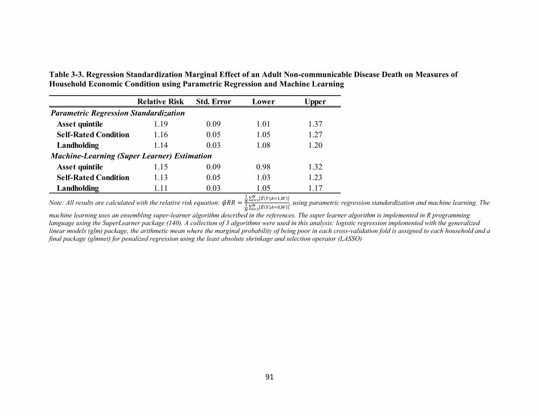
91
Table 3-3. Regression Standardization Marginal Effect of an Adult Non-communicable Disease Death on Measures of
Household Economic Condition using Parametric Regression and Machine Learning
Note: All results are calculated with the relative risk equation: �̂�𝑅𝑅 =1
𝑁∑ [�̂�(𝑌|𝐴=1,𝑊)]𝑁
𝑖=11
𝑁∑ [�̂�(𝑌|𝐴=0,𝑊)]𝑁
𝑖=1
, using parametric regression standardization and machine learning. The
machine learning uses an ensembling super-learner algorithm described in the references. The super learner algorithm is implemented in R programming
language using the SuperLearner package (140). A collection of 3 algorithms were used in this analysis: logistic regression implemented with the generalized
linear models (glm) package, the arithmetic mean where the marginal probability of being poor in each cross-validation fold is assigned to each household and a
final package (glmnet) for penalized regression using the least absolute shrinkage and selection operator (LASSO)
Relative Risk Std. Error Lower Upper
Parametric Regression Standardization
Asset quintile 1.19 0.09 1.01 1.37
Self-Rated Condition 1.16 0.05 1.05 1.27
Landholding 1.14 0.03 1.08 1.20
Machine-Learning (Super Learner) Estimation
Asset quintile 1.15 0.09 0.98 1.32
Self-Rated Condition 1.13 0.05 1.03 1.23
Landholding 1.11 0.03 1.05 1.17

92
Table 3-4. Relative Risk Estimates for the NCD versus the Comparison group for three economic outcomes
Note: In the table, “Asset quintile” refers to being in the bottom two quintiles as measured by asset-based principal component analysis. “Self-rated economic
condition” refers to being in the poor or very poor group and “Landholding” refers to owning less than 50 decimals of land. A decimal of land refers to 1/100th
of an acre or 40.46m2. “Prime Age” here refers to those deaths to individuals aged 15-59 and “Old Age” refers to deaths to those aged 60 and above.
Relative Risk Lower Upper Relative Risk Lower Upper Relative Risk Lower Upper
Full Sample 1.19 1.02 1.39 1.03 1.26 1.10 1.03 1.17
Sex
Male 1.22 0.98 1.52 1.04 1.34 1.18 1.08 1.29
Female 1.16 0.91 1.48 0.94 1.27 1.01 0.93 1.10
Age
Prime Age 1.96 1.39 2.76 1.24 1.79 1.07 0.94 1.22
Old Age 1.04 0.83 1.30 0.93 1.19 1.11 1.03 1.19
Education
None 1.13 0.96 1.34 1.04 1.29 1.04 0.97 1.11
1-5 years 1.28 0.85 1.94 0.00 INF 1.30 1.12 1.51
6+ years 1.55 0.66 3.64 0.91 2.03 1.12 0.89 1.40
Marital Status
Single/Widow/Divorce 1.08 0.81 1.45 0.71 1.43 1.09 0.99 1.20
Married 1.26 1.03 1.54 1.22 1.08 1.38 1.12 1.03 1.22
Position
Head/Spouse 1.18 0.97 1.43 1.03 1.3 1.14 1.06 1.23
Non-Head/Spouse 1.18 0.86 1.63 0.86 1.28 1.03 0.90 1.181.05
1.16
0.99
1.36
1.01
1.16
Landholding
1.14
1.18
1.09
1.49
1.05
Asset quintile Self-rated economic condition

Version: June 1, 2014
93
Table 3-5. Log Binomial Regression for the Effect of an Adult Non-communicable Disease Death on Measures of Household
Economic Condition
Note: Significance: ***p<0.01, **p<0.05, *p<0.1. PA stands for prime-age, which is ages 15-59. All standard errors are clustered at the household level.
Asset quintileAsset quintile -
PA Interaction
Self-rated
condition
Self rated condition -
PA InteractionLandholding
Landholding - PA
Interaction
Intercept 0.85 1.60 1.94* 1.89 1.34 1.55
NCD death 1.19* 1.07 1.16** 1.09 1.14** 1.15**
Prime Age 0.74** 0.74** 0.86* 0.86 0.84** 0.84**
Female 0.99** 0.98*** 0.99*** 0.99** 0.99*** 0.99***
Age 0.55*** 0.55*** 0.83** 0.83** 0.76*** 0.76***
Education
1-5 years (ref. None) 0.26*** 0.27*** 0.43*** 0.44*** 0.65*** 0.65***
6+ years (ref. None) 1.69 2.06 1.30 1.34 2.09*** 2.14***
Marital Status
Married (ref. Unmarried) 2.94 3.40 1.23 1.18 1.17 1.23
Divorced (ref. Unmarried) 1.86 2.25 1.41 1.44 2.41*** 2.47***
Widowed (ref. Unmarried) 1.01 1.00 0.93 0.93 0.94 0.94
HH head/spouse 0.87 0.87 0.88 0.88 0.78*** 0.78***
Muslim 0.92*** 0.92*** 0.95*** 0.95*** 0.97*** 0.97***
Household size 1.31 1.38 0.80 0.81 0.42 0.42
NCD x Prime Age 1.70*** 1.33* 0.94
Log Likelihood -1216.67 -1212.17 -1863.08 -1861.32 -2203.54 -2203.18
Deviance 1355.33 1346.34 1582.16 1578.63 1255.09 1254.35
Num. obs. 2,491 2,491 2,491 2,491 2,490 2,490

Version: June 1, 2014
94
3.10 Figures for Chapter 3
Figure 3-1. Diagram of Study Design
Note: NCD stands for non-communicable disease. The 909 households with an NCD death were identified
from the demographic surveillance system run by the non-profit icddr,b. Causes of death were assigned by
verbal autopsy to international classification of disease version 10 (ICD-10) code, which was used to
identify all NCD deaths. Being poor or not was measured by three outcomes, asset index, self-rated
economic condition or total landholding.

Version: June 1, 2014
95
Figure 3-2. Pros and Cons of Different Measures of Economic Condition
1. Asset index with PCA Pros: Standard for measuring wealth
in the absence of consumption and
price data.
Cons: May no correlate well with
consumption. May not accurately
reflect the prices of assets.
2. Self-rated condition Pros: Captures broader components
of economic well-being and effects
not related to asset ownership.
Cons: Non-poor households may
underreport economic condition.
Household respondents may not be
able to compare to the entire area.
3. Landholding Pros: Proven as a good measure of
economic status in rural Bangladesh.
Cons: May be less important as
economies shift away from
agriculture. Threshold for poor status
may be arbitrary.
Measure of Economic Outcome Pros and Cons

Version: June 1, 2014
96
Figure 3-3. Causes of Adult NCD Death in Matlab in 2010
Note: Causes of death identified by ICD-10 code based on underlying cause of death as recorded by verbal
autopsy. The total number of deaths are 909. NCD stands for non-communicable disease. Other represents
other non-communicable diseases. Deaths from Injury are excluded.
0
50
100
150
200
250
300
350N
um
ber
of
Dea
ths

97
Chapter 4. Evaluating Household Coping Strategies after an Adult Non-Communicable Disease Death in Rural Bangladesh
4.1 Abstract
With the emerging burden of non-communicable diseases (NCD) in low-income
countries, understanding how the illness or death of an adult household member affects
the economic condition of a household is important for mitigating health-related poverty.
After an adverse health event, households adopt coping strategies to offset the effects of
the economic consequences such as high medical expenditures or lost human capital. The
adverse event, or health “shock” may impose a large economic impact on households and
coping strategies represent intermediate pathways through which these effects occur. This
research looks at how households cope after an adult NCD death in the rural, low income
area of Matlab, Bangladesh. Household and individual-level characteristics are explored
as determinants using certain coping strategies, which fall into the categories of financial,
demographic and behavioral coping. Adult NCD deaths in the year 2010 were identified
through the Matlab surveillance system and surviving household members were
interviewed in 2012 to identify which coping strategies were used. A multivariate logistic
regression is used to examine the determinants of coping within the group of households
with deaths and in relation to a comparison group of households with no deaths in 2010.
An econometric difference-in-difference (DiD) approach is used to examine the level of
human capital replacement with objective measures of household composition. The most
common coping strategy among households after the death was the reduction expenditure
on basic items such as food and utilities. Having a prime age death led to an increase in

98
the most number of coping strategies, four out of ten. Being poor prior to the death
appeared lead to restricted options for financial coping as these household were less
likely to use such strategies. The DiD results show that overall, households with adult
NCD have modest levels of replacement of human capital. More replacement is seen for
prime age deaths in terms of recruiting adult women into the household, which may be
due to a higher likelihood of males re-marrying females that are of reproductive age. The
results from this work may be used to inform further poverty-reduction and NCD health
programming in this rural area of Bangladesh and may inform the creation of policies in
other rural, low-income settings as well.
4.2 Introduction
The emerging burden of non-communicable disease (NCD) in rural, low income settings
may have significant adverse impact on the livelihoods of populations living in these
settings. An adult death in a household from an NCD may be considered a health “shock”
that poses costs and has consequences for the economic well-being of the household.
There may be high levels of health expenditure surrounding the death and the death itself
could pose a loss to household human capital, especially if it’s to a prime, working age
member. Households, however, can offset the cost of the health shocks by engaging in
coping activities. These may include adjusting household finances, changing the
composition of the household to shift human capital or engaging in other behaviors,
which impact household economic condition.
In rural Bangladesh, there has been a rise in proportion of the mortality burden from
NCDs in adults (5). In Matlab, a rural sub-district in Bangladesh where intensive

99
maternal and child health services have been conducted for decades, there has been an
exceptional rise in the burden of adult and NCD mortality. Research using data from
Matlab has shown that there is a socioeconomic gradient in NCD outcomes and risk
factors where the worse off are more likely to have elevated risk factor levels and worse
mortality (18). Understandings of the socioeconomic gradient, however, provide only a
partial picture of the relationship between health and wealth. Adverse health events pose
costs to households and may cause either short or long-term impacts to overall household
wealth. In Matlab, this has been documented in terms of the economic impacts from
maternal health complications, but it has not been as well studied for adult outcomes
from NCDs (100).
The impacts of NCD-related health shocks for households may also been seen by the
coping strategies, which households use to adjust for the effects of illness or death (148-
150). One coping strategy that may be harmful is a reduction in basic household
consumption. This may have severe effects for the development of children in the
household and for the health of adults as well. Additionally, the adoption of high interest
loans that cannot be paid off easily may damage a household’s financial prospects. Other
potentially harmful coping strategies include: spending down savings or selling assets,
experiencing a decrease in social safety net transfers or having a member sacrifice
education to take up a job or work in the household. All of these coping strategies reduce
the resources of households, which may make them more vulnerable to future shocks.
Households in rural Bangladesh have been seen to use many types of coping strategies
following a health shock (151). Rural Bangladesh also provides an understanding of

100
coping in terms of micro-lending because of the ubiquity of microfinance institutions
(MFI) in the country (121, 145).
The impact from harmful coping strategies may also be related to characteristics of the
household before the shock occurs. For instance poor households may be more likely to
use harmful coping strategies because safer ways of adjusting to the cost of the shock are
not available. Additionally, the characteristics of the deceased may determine which
coping strategies are used as a prime age (working age, 15 to 59 years old) death or death
to a higher ranking member of the household could mean a larger economic consequence
for the household. In the patriarchal societal structure in Matlab, where most of the
primary income earners are males, a death to a male versus a female member would lead
to a stronger coping response in terms of recruiting another prime age male into the
household, which has been seen in studies in Tanzania (99). Alternately, this effect could
be reversed in a setting such as Matlab where reproductive age females are recruited into
the household by males, but female widows are not able to re-marry another male. Deaths
also impose a change in the household composition which may require coping strategies
to change household size further or change the household labor structure (112). In
response to a health shock from a death, households may either recruit new members into
the household or send members away. Additionally, the duration of morbidity prior to the
death may be an indicator for the severity of the health shock and for whether households
spent much time in a prolonged, depressed state prior to the death.
The objective of this research is to understand how households cope ex post after an adult
NCD death in rural Bangladesh. Special attention is paid to coping strategies that may be

101
harmful for households in terms of long-term poverty impacts. Individual and household
level determinants of using coping strategies are also examined both within a group of
NCD deaths and in relation to a comparison group of households with no deaths.
4.3 Literature Review for Understanding the Health and Wealth
Link in Terms of Coping Strategies
The way in which households handle economic impacts from NCDs is of interest as
NCDs become more prevalent. In several low and middle-income country examples,
studies have looked at household coping strategies in response to health shocks both
before (ex ante) and after (ex post) the shock occurs (152-154) (118). Coping
mechanisms that households engage in following a health shock may have important
implications for understanding poverty as well. Coping itself may impose a direct or
indirect cost on households that extends beyond the cost of the illness itself (43). The
adverse effects of coping may pose a significant cost to households in the long term and
cause the household to become more vulnerable to future shocks and impoverishment
(155-157). Coping, however, is not inherently bad for households will occur to some
degree after any shock to a household.
Coping in rural Bangladesh has been looked at previously and idiosyncratic shocks from
health events are found to be quite important (158). When households are faced with a
health shock, there are several financial responses that are available to them. These
include strategies such as reducing expenditure on basic items. This has been looked at in
terms of expenditures on food for the household (100). While reduced expenditures may

102
be for either a short period of time after the shock, it could also have longer term impacts
on the well-being of children.
Another important coping strategy for households is to borrow money from MFI’s. The
ubiquity of MFI lenders means there is a high rate of borrowing for such a rural, low
income area (121, 158). There has been mixed evidence about the effectiveness of
microfinance for mitigation economic risk and raising households out of poverty, but a
recent review found that over the long-term it appears to be helpful (146, 159). In rural
areas of South Asia, though, there is still a high level of reliance on informal borrowing
sources such as friends, relatives and moneylenders (160). Borrowing from both formal
and informal sources has been seen to be detrimental to households when loans are given
at high interest rates (98).
In addition to borrowing, households may also cope by selling asset or spending savings
(98). This may also lead to higher vulnerability since households are less able to adjust
for future shocks. In rural areas, some studies have shown that selling productive assets
such as livestock is a common form of coping (99). Coping in this manner indicates that
there is a lack of formal safety net options available.
A household death means a loss of human capital for the household. The death may result
in lost income through the reduction in labor supply (158). A decrease in human capital is
most detrimental for households with prime age deaths. Several studies have attempted to
look at whether or not households are able to replace human capital after a death through
recruitment of new prime age members into the household. One study in Tanzania found
that household do not replace adult human capital very well. In comparison with a control

103
group, they found that the loss of a prime age adult led to only 20% of households
replacing the lost human capital (99).
Beyond household finances and labor supply, there are many other strategies that
households may use to cope with shocks. Two of these that are of interest in rural areas
are the effects on marriage and education. Having a household member marry early may
be another way to adjust the human capital in the household. Marriage of a daughter early
would then mean one less person in the household and linkages to another social network
where resources can be shared; however, early marriage’s harmful effects in terms of
reduced education and labor force participation for the female have been well-
documented (161). In terms of education, households with deaths to prime age members
may be more likely to have a school-aged child leave education early and begin working
(100). Given the strong positive relationship that is seen between education and later life
health and economic condition. This reduced level of education will have resonating
effects for the rest of the child’s life.
Understanding coping strategies in terms of the initial resources available to households
is also important. Access to coping strategies is likely not just an issue of household
preference, but is more likely to be based on access based on a household’s status or
wealth (162). Previous work looking at household coping from mortality shocks have
found that resource-rich households have more access to resources and social capital and
can thus rely more on private transfers. The resource-poor, having less social capital,
networks of wealthy donors and trust for repayment rely more on credit (163). In terms of

104
human capital replacement, households that were poor before a prime age death have
been shown to replace human capital at lower rates (99).
4.4 Data
4.4.1 Identifying How Households Cope
The data for this study comes from the routine surveillance system from Matlab,
Bangladesh administered through the International Center for Diarrhoeal Disease
Research in Bangladesh (icddr,b). This is an ongoing surveillance system that has been
administered for several decades in this rural region. In addition to the routine
surveillance data, information is used from a survey designed to assess the economic
impacts from an adult NCD death. A version of this survey is found in the Appendix
7.1. The survey includes modules for demographic information of the household and the
household head, information about the NCD death and deceased individual and a module
to assess the coping strategies that a household reports using after a death. This survey
was administered in 2012 for the group of households experiencing an adult NCD death
in 2010 in Matlab. A similar survey for a comparison group of households with no death
in 2010 matched on the age, sex and village of the deceased individual was also
collected. Information on the household in the years prior to the death were obtained
from the routine Matlab surveillance data. Baseline demographic and socioeconomic
information was for the year 2009, the year prior to the identified NCD deaths.
Ten different coping strategies, considered to have important economic consequences for
households are included in addition to household composition broken down four different

105
ways. The ten strategies are classified into three coping categories: financial coping,
demographic coping and behavioral coping. The ten strategies that are used in this study
have been looked at in previous literature on coping analysis (158, 160, 163). These then
strategies are given in A-C below and the household composition variables are given in
D. All coping outcomes are described in further detail in the following sub-sections:
A. Financial Coping
1. Decline in expenditure on basic items.
2. Taking out a high interest institutional loan.
3. Taking out a high interest independent loan.
4. Selling household assets.
5. Spending household savings.
6. Having decreased transfers from social safety net programs.
B. Demographic Coping
7. Having someone move out of the household.
8. Having someone move in to the household.
C. Behavioral Coping
9. Having someone in the household marry early.
10. Having someone in the household leave education.
D. Household Composition
Household size
Total Males
Total Females
Total Children

106
4.4.2 Dependent Measures of Household Coping
The dependent variables of interest were the ten coping strategies that houses reported
using after an adult NCD death in 2010. These were coded as either a one or zero
depending on whether a household reported using the strategy or not.
4.4.2.1 Financial Coping
The decline in basic expenditure was defined as a reduction in spending on items such as
food and utilities in the one to two year period since the death. A further question asked
about whether households experienced a decline in expenditure on discretionary items,
but these results are not shown here. One limitation of this question is that the time when
the decline in expenditure on basic items occurred is not known. Households may have
experienced the decline immediately after the death or have an extended decline in
expenditure that lasted up to the time of the interview in 2012.
Detailed information was collected concerning any loans the households took out after
the death. Two types of loans were specified, institutional loans received from banks or
nonprofit organizations and independent loans taken from friends, neighbors, relatives or
moneylenders. For each household, information on up to two loans from each source
were collected. Loan information included the interest rate, length of the loan and the
collateral. For this study, only the information on the first loan in each category of
institutional or independent sources was used since there were very few households
reporting a second loan. High interest loans are also distinguished by whether the interest
rate was higher than the standard commercial loan interest rate of 13% (145).

107
Further coping strategies in the financial category included selling assets, spending
savings and having a decrease in the amount of transfers received form social safety net
programs. These variables all represent a decrease in the stock of financial resources or
income streams that are available to households.
4.4.2.2 Demographic Coping
The two strategies for demographic coping included having a member move out of the
household or having a member move in to the household. These were asked
independently, thus a household was able to report having used both strategies. For the
comparison group, it was asked whether a member had to move out or move in at any
time since 2009. One limitation from this question is that information about the person
that moved into or out of the household was not asked.
4.4.2.3 Behavioral Coping
Behavioral coping included two strategies of whether a household had someone marrying
early because of the NCD death or whether someone had to leave education to work or
attend to the household because of the NCD death. For the comparison group, this was
asked in terms of the entire reference period since 2009. These strategies also did not
collect further information about the characteristics of the person who either married
early or left education.
4.4.2.4 Household Composition
The analysis of coping in terms of household composition used the household roster in
the baseline year 2009, one year before the death, and two years after the death, at the

108
time the survey was collected in 2012. Dependent variables for this analysis included the
total adult members aged 15 and above and the total number of children, under age 15.
Total adults were looked at in aggregate and by sex and prime age status.
4.4.3 Independent Measures
Explanatory characteristics at the household level and for the deceased individual were
also examined to see how they were associated with individual coping strategies. At the
household level, baseline characteristics of the household size in terms of total members
and the age, sex and years of completed education of the head of the household were
included. A baseline indication of being poor or not, whether a household was in the
lower 40% of a self-rated 5 step ladder of economic condition distribution, or the lowest
2 steps, was also controlled for.
Explanatory variables for the deceased individual are used to give an indication of the
severity of the health shock and include the age, sex and position in the household. Age
here was a binary variable according to whether the individual who died was prime age
or not. Household position was also coded as binary, according to whether the individual
was the head of the household.
The time of severe illness of the deceased individual prior to their death was also used to
explore how a household coped after differing periods of severe morbidity that may put
the household in a depressed state prior to the death or lead a household to anticipate a
health shock from an NCD death, also called ex ante coping. To measure this, a disease
timeline was developed. Households were asked to identify the time of death of the

109
individual and to work backwards to develop the times of severe illness, non-severe
illness and disease onset. The time of severe illness was defined as: not being able to
work, go to school, or perform daily activities without assistance. Households indicated
the dates for each of these times and the measure was reported in years. For regression,
analysis a dummy variable was used for whether an NCD death was above or below the
median period of severe morbidity which was 120 days.
4.5 Analytical Framework
The percentage of households using each coping strategy is reported as well as the
percentage of households reporting using at least one strategy from one of the three
categories. Additionally, the extent to which households use multiple strategies or
multiple coping categories is also evaluated.
4.5.1 Multivariate Logistic Regression Analysis
In multivariate analysis, a logistic regression model was specified for each coping
strategy, Y, to examine which characteristics are associated with each coping strategy.
The regression model was run for just the population of households with an NCD death
to evaluate the determinants of coping conditional on having a death in the household.
This model was specified as follows:
𝑙𝑜𝑔𝑖𝑡(𝑌) = 𝛽0 + 𝛽1𝑋1 + ⋯ + 𝛽𝑛𝑋𝑛 (1)
In equation 1, the left-hand side of the equation, logit(Y), is the log odds that each coping
strategy was adopted and 𝛽0 is the intercept term. The vector X represents n number of

110
independent variables at the individual and household level. These include the individual
characteristics of the NCD death itself as well as a list of exogenous household controls.
The vector of coefficients, 𝛽1−𝑛, represent the change in the explanatory variable of
interest that relates to a unit change in the log odds of Y. All standard errors for equation
1 are clustered at the village level.
The likelihood of increased coping levels that are a result of the NCD health shock itself
is also of interest and may provide more understanding of the wealth impacts that result
from NCD health shocks. For this reason, the logistic regression model was also run with
a comparison group of households with no deaths. This model was specified according to
the following equation:
𝑙𝑜𝑔𝑖𝑡(𝑌) = 𝛽0 + 𝛿𝑁𝐶𝐷 + 𝛽1𝑋1 + ⋯ + 𝛽𝑛𝑋𝑛 (2)
Equation 2 similarly looks at Y as a dependent variable for household coping strategies
and the vector of X’s for individual and household level controls. The standard errors for
equation 2 are also clustered at the village level. This equation now incorporates a
dummy variable for whether a household experienced an NCD death or not, NCD. The
coefficient 𝛿 represents the log odds that a household used a particular coping strategy
after an NCD death in comparison to the counterfactual comparison group.
To understand how the odds of using a coping strategy may differ by the characteristics
of the death itself or whether the household was poor prior to the death, a series of five
equations that are extensions of equation 2, run with the entire sample of NCD death and
comparison households were implemented:

111
𝑙𝑜𝑔𝑖𝑡(𝑌) = 𝛽0 + 𝛿𝑃𝐴𝑁𝐶𝐷𝑃𝐴 + 𝛿𝑁𝑜𝑛−𝑃𝐴𝑁𝐶𝐷𝑁𝑜𝑛−𝑃𝐴 + 𝛽1−𝑛𝑋1−𝑛 (3)
𝑙𝑜𝑔𝑖𝑡(𝑌) = 𝛽0 + 𝛿𝐻𝑒𝑎𝑑𝑁𝐶𝐷𝐻𝑒𝑎𝑑 + 𝛿𝑁𝑜𝑛−𝐻𝑒𝑎𝑑𝑁𝐶𝐷𝑁𝑜𝑛−𝐻𝑒𝑎𝑑 + 𝛽1−𝑛𝑋1−𝑛 (4)
𝑙𝑜𝑔𝑖𝑡(𝑌) = 𝛽0 + 𝛿𝐹𝑒𝑚𝑁𝐶𝐷𝐹𝑒𝑚 + 𝛿𝑀𝑎𝑙𝑒𝑁𝐶𝐷𝑀𝑎𝑙𝑒 + 𝛽1−𝑛𝑋1−𝑛 (5)
𝑙𝑜𝑔𝑖𝑡(𝑌) = 𝛽0 + 𝛿𝐿𝑜𝑛𝑔𝑁𝐶𝐷𝐿𝑜𝑛𝑔 + 𝛿𝑆ℎ𝑜𝑟𝑡𝑁𝐶𝐷𝑆ℎ𝑜𝑟𝑡 + 𝛽1−𝑛𝑋1−𝑛 (6)
𝑙𝑜𝑔𝑖𝑡(𝑌) = 𝛽0 + 𝛿𝑁𝐶𝐷 + 𝛽1𝑃𝑂𝑂𝑅 + 𝛾𝑁𝐶𝐷𝑥𝑃𝑂𝑂𝑅 + 𝛽2−𝑛𝑋2−𝑛 (7)
Equations 3 through 7 show the variable for an NCD death with superscripts that
represent dummy variables for whether the death was to a prime age (PA/Non-PA)
person, a head of household (Head/Non-Head), the sex of the deceased (Fem/Male) or
whether the death had a prior long period of severe morbidity (Long/Short). Equation 7
keeps the same dummy variable for any NCD death as equation 2 but also includes a
dummy variable for whether a household was poor (POOR), which is interacted with the
variable for NCD death. All five of the equations include a vector of X’s for exogenous
controls and cluster the standard errors according to village.
4.5.2 Difference-in-Difference Analysis
To evaluate changes to household composition, an econometric difference-in-difference
(DiD) analysis with direct matching of the households with an adult NCD death to a
comparison group of households that had no deaths in 2010 is used. This approach
assesses the difference in the change to the number of adults and children present in the
household relative to this difference in the comparison group. The direct matching

112
ensures that potential confounders of household status are balanced at baseline and the
DiD approach accounts for time-variant and time-invariant unobservable factors of the
households by taking into account differences in the outcome variable both within and
between each group (99).
The DiD approach compares the mean difference between the NCD death and
comparison groups. Initially, the difference in the outcomes of household composition for
each group between the baseline year and two years post death is estimated (first
difference). These differences are then compared to each other (second difference) with
the following equation:
𝐸(𝛿) = 𝐸(∆𝑌𝑁𝐶𝐷) - 𝐸(∆𝑌𝐶𝑜𝑚𝑝) (8)
In equation 8, the term E(∆𝑌) is the change in the expected value of the composition
variable for each of the NCD and comparison groups. The E(𝛿) term denotes the DiD
estimate of the change in the expected value of the composition variable of interest.
To assess the significance of the DiD estimate in equation 8, an ordinary least squares
(OLS) regression model is specified:
𝑌𝑡 = 𝛽0 + 𝛽1𝑁𝐶𝐷 + 𝛽2𝑇𝑖𝑚𝑒 + 𝛽3𝑁𝐶𝐷 ∗ 𝑇𝐼𝑀𝐸 + 휀𝑡 (9)
In equation 9, Yt is the composition variable of interest at time t. 𝛽0 is the intercept, 𝛽1and
𝛽2 are the main effects of the change in composition explained by a dummy variable
representing whether a household had an NCD death (NCD) and the time period (TIME).
The coefficient for the interaction between having an NCD death and time, 𝛽3, represents

113
the equivalent of the DiD estimate provided in equation 8, which now includes a standard
deviation, clustered at the village level, for assessing significance.
To further assess the DiD estimates, equation 9 is also run with a vector of assumed
exogenous household controls. This is given in equation 10 below:
𝑌𝑡 = 𝛽0 + 𝛽1𝑁𝐶𝐷 + 𝛽2𝑇𝑖𝑚𝑒 + 𝛽3𝑁𝐶𝐷 ∗ 𝑇𝐼𝑀𝐸 + 𝛽4−𝑛𝑋4−𝑛 + 휀𝑡 (10)
The vector of X’s in equation 10 represents these controls. Characteristics of the death are
assessed with dummy variable in two separate equations.
𝑌𝑡 = 𝛽0 + 𝛿1𝑁𝐶𝐷𝑃𝐴 + 𝛿2𝑁𝐶𝐷𝑁𝑜𝑛−𝑃𝐴 + 𝛽1𝑇𝐼𝑀𝐸 + 𝛿3𝑁𝐶𝐷𝑃𝐴 ∗ 𝑇𝐼𝑀𝐸 +
𝛿4𝑁𝐶𝐷𝑁𝑜𝑛−𝑃𝐴 ∗ 𝑇𝐼𝑀𝐸 + 𝛽2−𝑛𝑋2−𝑛 + 휀𝑡 (11)
𝑌𝑡 = 𝛽0 + 𝛿1𝑁𝐶𝐷𝐹𝑒𝑚 + 𝛿2𝑁𝐶𝐷𝑀𝑎𝑙𝑒 + 𝛽1𝑇𝐼𝑀𝐸 + 𝛿3𝑁𝐶𝐷𝐹𝑒𝑚 ∗ 𝑇𝐼𝑀𝐸 +
𝛿4𝑁𝐶𝐷𝑀𝑎𝑙𝑒 ∗ 𝑇𝐼𝑀𝐸 + 𝛽2−𝑛𝑋2−𝑛 + 휀𝑡 (12)
Equations 11 and 12 show the DiD regression equation with dummy variables for
whether a death is to a prime age (PA/Non-PA) individual or to a male or female
(Fem/Male). The coefficients for the dummy death variables interacted with time 𝛿3and
𝛿4represent the DiD estimates of interest.
4.6 Results
Descriptive information for the study population is provided Table 4-1. The top half of
the table lists the household-level variables that are considered controls for the analysis.

114
The households in each of the groups appear balanced in all of the characteristics. The
variable for being poor in this section is a binary indicator of whether a household
responded to the 2012 survey saying that the household was in the first two self-rated
quintiles either before the death for the NCD group or in 2009 for the comparison group.
44% of the NCD households and 43% of the comparison households rated themselves as
poor, giving us confidence in the matching process. This is higher than the rural poverty
rate provided by the World Bank in 2010 which was 35.16% (164).
The second half of the table includes information at the individual level. The information
for age and sex was used in the original direct matching for the selection of the study
population. The population appears to be evenly balanced except for the condition of
whether the individual was the head or spouse of the head of the household. For this
variable, the comparison group has a 7% more household heads and spouses. The length
of severe illness leading up to an NCD death is only applicable for the NCD group and
was found to be around a third of a year (SD 1.2 years).
4.6.1 Results for How Households Cope
Table 4-2 lists the percentage of households that reported using each coping strategy and
each coping strategy category for each of the groups. For the individual coping strategies,
there are some stark differences. In the category of financial coping strategies, the
households experiencing adult NCD deaths are much more likely to report having a
reduction in expenditure on basic household items. This is the most prevalent form of
coping reported by the NCD group, with 43% of households saying they reduced basic
expenditure. The NCD households are also less likely to have a high interest institutional

115
loan or high interest loan from an independent source. A lower percentage of NCD
households report spending savings or selling assets, but a higher percentage report
having a decline in social safety net transfers. For the financial coping category overall, a
similar percentage of each group, about half, report using at least one version of financial
coping during the time period.
For the two strategies classified as demographic coping, the NCD households were much
less likely to report having someone move out than the comparison households.
Alternately, the NCD households were more likely to report having someone move in
than the comparison households though moving out was more common for both. Overall
for the category, the comparison households had twice as much demographic coping than
the NCD households which was mainly driven by high levels of moving out in the
comparison group. The least differences between groups were seen in the behavioral
coping strategy. For both having someone in the household marry early and for having
someone in the household leave education, about 1.5% of the households reported using
the former strategy and about 5% reported using the latter strategy. Overall, 5.6% and
5.7% of the NCD and comparison households reported using a behavioral coping
strategy.
Table 4-3 lists the results for how many coping strategies and coping categories each
household used among those that we observed. These were relatively stable for both
groups. The NCD death households were more likely to use zero or one strategy, and the
comparison households were more likely to use 2 or more. A similar pattern was seen for
the categories, where comparison households were more likely to use more coping

116
categories although the differences appear minimal. Table 4-3 also shows that
households are most likely to use zero or one coping strategy or coping strategy category
with a rapid decrease in the percentage of households using more than one strategy.
The differences in the coping strategy use show that there may be limitations to the data
in terms of how the information for the coping strategies was collected. In the survey
instrument, the NCD households were asked about coping strategies “as a result of the
NCD death”, while the comparison group was asked about whether the coping strategy
was used at any point during the time period. This may be one reason why there are
several coping strategies that are much more common for the comparison group. Using
administrative data would be one way to test for this bias in the results. An attempt to do
this with information for household composition is done with the DiD analysis
subsequently in this paper.
4.6.2 Results for Multivariate Determinants of Coping
Multivariate results for the nine coping strategies are provided in Tables 4-4 and 4-5.
Table 4-4 shows the results of the logistic regression results for just the population of
households with an adult NCD death. The regression models included all of the
household and individual level variables and standard errors clustered at the village level,
although only the household-level variable for being poor is shown in Table 4-4. For the
category of financial coping, it is seen that a male death or a death with a long period of
severe morbidity leads to a significantly higher likelihood of a household reducing
expenditure on basic items. In terms of taking out high interest loans. Being poor leads to

117
a significantly higher likelihood of taking out institutional loans and a long period of
severe morbidity lead to a significantly higher odds of an independent loan. A household
being poor was significant and inversely associated with spending savings or selling
assets. A household with a prime age death was more likely to sell assets. A decrease in
social safety net transfers, which are provided through national-level government
programs, was significantly positively associated with a death to a female.
There were not many variables significantly associated with reporting demographic
coping. Having a prime age death was positively associated with having a household
member move out of the household and no variables were significant for having someone
move in. The two strategies for behavioral coping showed more significant associations.
Households with prime age deaths were significantly more likely to both have someone
marry early and to have someone leave education. In addition, female deaths were
strongly associated with having a household member marry early and having a death
preceded by a long period of severe morbidity was positively associated with having
someone leave education.
Overall, Table 4-4 shows that having a prime age death is positively associated with the
most number of coping strategies, four, and with coping strategies in each of the three
categories. Having a long period of severe morbidity was also significantly positively
associated with three coping strategies in two out of the three categories. Being poor prior
to the death was positively associated with taking out a high interest institutional loan but
negatively associated with reporting spending savings or selling assets. Interestingly, the
position of the deceased person in the household did not show any significance.

118
Table 4-5 shows the results for the likelihood of reporting coping for the households with
a death in relation to the comparison group of households with no deaths. The rows each
represent separate regressions with all household controls included and standard errors
clustered at the village level. For the category of financial coping, an NCD death is more
likely to lead to decline in basic expenditures compared to a comparison group, which is
consistent regardless of the characteristics of the death or the economic condition of the
household prior to death. This is seen with the large positive and significant coefficients
in the first column and the non-significant coefficient on the interaction term with being
poor. The only other financial strategy with large positive association with NCD death is
reporting a decline in social safety net transfers. This strategy also shows differences by
death characteristics where households with deaths to older individual and females more
likely to report a decline. The other four coping strategies in the financial category,
having a high interest institutional or independent loan; spending savings or selling
assets, show many significant inverse associations with having an adult NCD death. The
interaction term for being poor prior to death is only significant for the strategy of
spending savings where poor households with NCD deaths are less likely to use this
strategy.
The two demographic coping strategies in Table 4-5 show opposite relationships to
having an NCD death. Reporting someone moving out of the household is negatively
associated with an NCD death for many of the models and does not appear to differ much
by the characteristics of the deceased. Reporting having someone move into the
household is positively associated with an NCD death for many of the models and

119
appears especially strong for having a prime age death. Neither of the demographic
coping strategies are associated with the initial economic status of the household.
For the behavioral coping category, having a prime age NCD death is positively
associated with reporting having a member marry early. None of the other characteristics
of the deaths are significant for this strategy, including having a female death, which was
a strong predictor when looking only at the NCD group. Having any adult NCD death
was not associated with reporting having someone leave education, but in several
situations, such as having a female death or death to an older member, households were
less significantly less likely to report having someone leave education.
Overall, when compared to a groups of households with no NCD death, the coping
strategies of reducing basic expenditure and having reduced transfers from social safety
net programs appear to be the most likely coping strategies that a household with an NCD
death uses. By characteristics of the deceased, some important differences are seen when
the death is to a prime age individual, which leads to a higher likelihood of having
someone move into the household or marry early. The initial economic condition of the
household does not play as important of a role for reporting using strategies, but there is
some indication that poor households have less options available to them.
4.6.3 Difference-in-Difference Results
The results for the DiD analysis are provided in the four tables, Tables 4-6 to 4-9. Each
of the tables shows the ordinary least squares regression model results for changes to the
four outcomes of household composition. The models only report the DiD estimate on the

120
NCD death variable of interest and standard errors clustered at the level of the village. In
each of the four tables, model 1 shows the results for the unadjusted regression with any
NCD death and model 2 shows the results for the model with any NCD death including
all of the household controls. Models 3 and 4 also include the exogenous household level
controls and include dummy variables for the prime age status of the deceased and for the
sex of the deceased. The prime age status is included because it has been seen to have
important impacts on household economic condition and likelihood of using coping
strategies. The sex of the deceased is included to explore the impact on the household
composition variable, which also include a breakdown by sex.
Table 4-6 shows the DiD results for change in total household size. In both the
unadjusted model 1 and model 2, which adjusts for household controls, the total change
in the household size is -0.7 and significant. This means that on average, households are
able to attract new members. A DiD estimate of -1 would mean perfect non-replacement
and a DiD estimate of zero would mean perfect replacement. The estimate of -0.7 means
that for every 100 households with deaths, 30 of them are able to attract new members.
By prime age status and sex of the deceased, it’s also seen that households are more
likely to attract members with a prime age death and with a female death. The prime age
death shows a positive DiD estimate of -0.45 meaning that for every prime age death,
over half of them are able to attract new members. This is in contrast to a non-prime age
death where the DiD estimate of -0.77 means that less than half, or 23 out of 100
households with these deaths attract new members.

121
In Table 4-7, the results are shown for the change in total adult males. The DiD estimate
is lower here, about -0.49 for the unadjusted and adjusted estimates in models 1 and 2.
This is consistent with the results in Table 4-8 showing that the DiD estimate for change
in total females is -0.31 in the unadjusted and adjusted model. The larger loss in males is
likely because of the higher number of male deaths in the sample. An interesting
difference between the replacement of male and female adults is seen by comparing the
DiD differences for prime age and non-prime age deaths for the two outcomes in Tables
4-7 and 4-8. While the prime age status of the deceased has no bearing on the change in
total males, households with prime age deaths are more likely to replace total adult
females. This is seen by the DiD estimate closer to zero for prime age deaths in Table 4-
8. Model 4 for the changes in numbers of males and females according to the sex of the
deceased is consistent with each model, showing significant declines in males and
females matching the sex of the deceased.
Table 4-9 shows the change in total children in the household given an adult death. The
unadjusted and adjusted models both show marginally significant increases in total
children after a death to the household. The positive DiD estimate means that for every
100 households, 10 of them will add one child after a death. This result also changes
depending on whether the age or sex of the deceased member. Households with a death to
a non-prime age member see a significant increase in the number of children with a
positive DiD estimate of 0.13 and households with deaths to females see a positive
significant DiD estimate of 0.23. This means that for 100 households with an old age
death or a 100 households with a female death, approximately 13 and 23 of them will add
one child after the death.

122
In sum, the DiD analysis shows that households moderately replace human capital after
an NCD death and consistent with the multivariate regression results, a prime age death is
more likely to lead to human capital replacement. This is mainly driven by the
replacement of adult females after a prime age death. There is some evidence that
households balance dependency ratios by replacing children after an old age death. A
considerable increase in the number of children after a female death is an interesting
result that should be explored further.
4.7 Discussion
The findings show that after an adult NCD death, households cope through the reduction
in expenditure on basic items such as food and utilities. This is seen for the models using
just the NCD death sample and for the whole population, including a counterfactual
comparison group. Reporting a reduction in expenditure drives the results that most
households cope with only one of the ten strategies in this analysis and usually through
financial means. A reduction in basic household expenditure is important and it should be
studied further to see if there are any long-term effects for the household, even if the
short-term reduction in expenditure is able to be managed. This has especially been
proposed when reductions in basic expenditure affect the diet of children (100). There is
also worry that reductions to household expenditure may disproportionately affect the
lower status members of the household. Because Matlab is a patriarchal society, this
means that the females may be affected more. A reduction in basic expenditure is also
positively associated with longer periods of severe illness and with deaths to male
members. Both of these characteristics could be considered indicators of the severity of
the shock. For the former, a death to a male member means more repercussions for the

123
household while a longer period of severe morbidity means a higher cost as a result of
medical expenditures and reduced human capital.
In addition to the sex and period of severe illness deaths to prime age household members
also indicate that the impacts of the shock will be more severe. This is consistent with the
literature looking at health shocks from all forms (e.g. self-reported illness episodes) but
also health shocks from death where a prime age death represents a permanent loss of
human capital (99, 129). Prime age deaths are positively associated with four out of the
ten coping strategies representing all three coping categories: financial, demographic and
behavioral. The positive relationship of a prime age death with coping due to selling
assets is troublesome if those assets represent productive items that households use for
income generation. Prime age deaths have been shown to lead to the selling of such items
as livestock in previous research (97). One limitation of this research is that the type of
assets that were sold is not ascertained. The coping due to selling of assets means that
formal financial coping mechanisms, such as insurance and safety net programs are not
adequate to completely offset the costs of the shock when there is a prime age death.
Another finding of interest is the changes in how households cope after an NCD death
depending on a priori economic condition. Being in the bottom 40% of a self-rated
economic condition led to a positive relationship with taking out a high interest
institutional loan. While not completely explanatory, this finding may be consistent with
previous work showing that the poor are less likely to have informal networks such as
friends or family from which they can smooth the effects of a health shock (165). The
ubiquity of microfinance institutions in rural Bangladesh make this a troublesome

124
finding. Poor households incurring high interest loans are may be caught in a poverty trap
that worsens their economic situation. There are also indications that households that are
poor have a much more limited set of other financial coping options available. This is
seen with inverse relationships with spending savings and selling assets. This intuitively
makes sense and has been seen in other studies in low income countries (158, 166). The
limited palette of option for the poor, though, further emphasizes the need for affordable
coping options for these households.
The results from the DiD analysis that looks at objective measures of household
composition finds that there is moderate replacement of household members after an
adult death. The finding that only 30% of households replace human capital is consistent
with the range of 20% provided by a study looking at death shocks in Tanzania (99).
Households tended to be more likely to replace female human capital after a prime age
death than they were male human capital. This is inconsistent with theories of higher
values of male human capital in the area and should be explored further. This The DiD
results are also consistent with the multivariate regression using a comparison group.
These results found that households with any NCD death were more likely to report
having someone move into the household than the healthy group. Further, likelihood of
reporting having someone move in increased for prime age deaths and deaths with longer
periods of severe morbidity. This may indicate that households with prime age deaths and
with deaths that can be anticipated gives households a higher likelihood of anticipating
the effects of health shocks and taking measures to offset the effects (99).
125
4.7.1 Policy Implications
The understanding of the coping strategies that households use after a health shock may
provide several insights for policy. Importantly, the large percentage of households
reporting reductions in expenditure on basic items means that households are not insured
against the effects of health shocks from adult NCD deaths. This has been found to also
be the case in an important work in Indonesia that also finds households lack the ability
to smooth consumption and that more severe effects from chronic illness (20). The
finding from this work means that there will need to be new creative ways of providing
risk protection to households experiencing health shocks so that they do not need reduce
basic expenditure. The rural areas of Bangladesh have a prevalence of micro-lenders and
these have been shown to effective mechanisms for reducing the impact of health shocks
(121). Further incorporations of community based health insurance or building micro-
insurance packages into the current micro-lending options could be directions for
developing these mechanisms. There have been some recent attempts to do this, however,
the results show that the demand for micro-insurance is not strong and that the informal
economy has a large role to play (147).
A further direction for policy is through implementing health services in the region that
are geared towards NCD prevention and management. The result that a prime age death
leads to higher levels of potentially harmful coping strategies was found in these results
and is consistent with previous work for health shocks in other settings. Prime age deaths
should be equated to premature deaths, which are a concern for global efforts to scale up
the attention to NCDs. Matlab has a history of being at the forefront of implementing

126
large-scale health programs in a rural, low income setting. Providing services and
programs to address the emerging burden of NCDs should be adopted as a priority goal.
4.7.2 Limitations
A limitation of this work is that the setting in Matlab is not necessarily generalizable to
other rural, low income settings in other countries, or even in Bangladesh (78). This study
was possible because of the availability of data on NCD prevalence, mortality and
associated economic impacts. Matlab has reliable surveillance data for a rural, low
income setting and the deaths from NCDs can be individually identified and linked to
household information and socioeconomic status characteristics. The pros and cons of
using information from Matlab for broader generalizations have been previously noted.
A further major limitation of the analysis of coping mechanisms may be that our survey
itself induced bias for household reporting of coping strategies that signal hardship for
the household. This may be further exacerbated by the fact that the survey was done two
years after the death and thus recall of the death and post-death experience could be
reported as more severe than it actually was. The potential for biased reporting of the
impacts of a health shock from adult NCD death would mean that these conclusions
overestimate the broad economic costs of NCD deaths. In the DiD analysis that uses
household composition and comparison group, much of this bias is removed by using an
objective outcome, so it is encouraging that there is consistency with the subjective
reporting.

127
4.7.3 Future Research
This work motivates future research to better understand the coping mechanisms that
households use in terms of the actual monetary benefit that they provide. This could
include a research protocol to understand better the patterns of health utilization and out
of pocket health expenditures resulting from a health shock and how coping mechanisms
offset the costs of the shock in the short and long term. Understanding social mobility in
terms of changes in socioeconomic status and which coping strategies are more likely to
be associated with improving economic conditions over time would also be important.
Lastly, more implementation research about the use of formal and informal borrowing
mechanisms, specifically focusing on the behaviors of the poor will be important for
understanding coping and poverty traps in a rural, low income setting such as Matlab.
4.8 Conclusion
This study examines how households cope in terms of financial, demographic and
behavioral strategies after an adult NCD death in rural Bangladesh. The adult NCD
mortality burden is rising in this area, and studies have proposed that there is a potential
for large economic consequences for households. The results from this work show that
households with adult deaths engage in coping strategies that may have harmful impacts.
Households are most likely to use financial strategies such as reducing basic expenditure,
but they also deplete financial stocks and take on high interest loans. Policies that
develop formal financial protection tools for rural households need to be further
developed to prevent deleterious coping activity. Adult NCD deaths to prime age
household members are also shown to cause significant economic consequences to

128
households. The importance of prime-age deaths has been found previously in the
literature, but to our knowledge has not been explored with NCDs in low income settings.
This provides further justification for scaling up health policies that address the emerging
burden of NCDs in rural Bangladesh since premature deaths represent tragic and costly
losses for households.

129
4.9 Tables for Chapter 4
Table 4-1. Descriptive Information for Study Population at Baseline
Note: Poverty is defined as being in wealth quintiles 1 or 2, based on PCA of assets in 2005. MFI membership (microfinance institution) is defined as being a member in 2005. Length of severe illness is defined as the period when the deceased individual was no longer being able to work, go to school or perform daily activities without assistance.
NCD death Comparison
Mean (SD)/Proportion Mean (SD)/Proportion
1. Household-level Control Variables
Household size 6.18 (2.70) 6.23 (3.02)
Head Age 61.76 (13.92) 62.62 (13.72)
Head Female 0.23 0.23
Head Education 2.84 (3.69) 2.87 (3.59)
Muslim 0.85 0.87
Poor 0.44 0.43
2. Individual-level Variables (Deceased Individual and Matched Individual)
Age 67.71 (12.72) 67.33 (12.33)
Prime Age (%15-59) 0.21 0.21
Female 0.45 0.45
Head/Spouse of Head 0.66 0.73
Length Severe Illness (year) 0.36 (1.18) NA
N 856 1695
Variable

130
Table 4-2. Prevalence of Coping Strategy Usage for Study Population
Note: Decline in basic expenditure refers to a reduction in spending on food and utilities. A high interest loan refers to one with an interest rate above 13%. An institutional loan is a loan from a bank or a non-profit organization. An independent loan is a loan from friends, neighbors, relatives or moneylenders. Spending savings or selling assets is whether the household had to do so after the death. A decline in social safety net transfers is whether there is any decline in transfers. Moving in or moving out is reporting having a person move in or out of the household after the death. Marry early is having someone marry early after the death and leave education having someone leave current education to enter the workforce or attend to the household after death.
% Using Strategy % Using Category % Using Strategy % Using Category
1. Decline in basic expenditure 43.1% 53.4% 7.9% 51.2%
2. High interest institutional loan 6.8% 10.3%
3. High interest independent loan 1.1% 2.5%
4. Spend Savings 8.1% 33.0%
5. Sell Assets 4.2% 11.6%
6. Social Safety Net decrease 1.8% 0.2%
7. Move out 3.2% 5.6% 11.2% 11.9%
8. Move in 2.8% 1.9%
9. Marry early 1.6% 5.6% 1.4% 6.8%
10. Leave education 4.6% 5.7%
Comparison (N=1695)
Category
Financial
Demographic
Behavioral
NCD death (N=856)
Coping Strategy

131
Table 4-3. Percentage of households reporting multiple coping activities
Note: The number of strategies is the total number out of a maximum possible of ten strategies. There are three
categories of coping, which include Financial, Demographic and Behavioral coping strategies. Financial coping
includes: reducing basic expenditure, taking out a high interest loan from a formal or informal source, selling
assets, spending savings or having a decline in social safety net transfers. Demographic coping includes: having
someone move out or movie in to the household. Behavioral coping includes: having someone marry early and
having someone leave education early.
NCD death (N=856) Comparison (N=1695)
Number of Strategies % Using % Using
0 42.3% 41.6%
1 42.0% 38.0%
2 12.4% 14.9%
3 2.9% 4.7%
≥4 0.3% 0.8%
Number of Categories
0 42.3% 41.6%
1 51.5% 48.7%
2 5.4% 8.0%
3 0.8% 1.8%

132
Table 4-4. Logistic Regression on Coping Strategy Use for Households with NCD Deaths
Note:
***p < 0.01,
**p < 0.05,
*p < 0.1. Poor is defined as being in quintiles 1 or 2 of self-rated economic condition in 2009. All models here include controls for
household-level information. Prime age refers to being in the age group 15-59 in 2010. Long Severe refers to the natural log of the length of severe illness.
Standard errors are clustered at the village level.
Basic
ExpenditureInstitutional Loan
Independent
LoanSpend Savings Sell Assets
Decrease Soc.
Safety TransfersMove Out Move In Marry Early Leave Education
(Intercept) -0.307 (0.501) -2.479 (0.892)*** -2.558 (2.650) -2.302 (0.850)
***-3.022 (1.113)
***-3.749 (2.170)
*-4.774 (1.527)
***-3.911 (1.300)
***-5.126 (1.255)
***-1.948 (0.958)
**
Prime Age 0.119 (0.196) -0.542 (0.463) 0.527 (0.910) -0.047 (0.373) 1.004 (0.417)** -1.332 (1.239) 0.886 (0.521)
* 0.420 (0.521) 1.243 (0.540)**
0.830 (0.417)**
Head -0.190 (0.212) -0.105 (0.489) 0.805 (1.045) 0.124 (0.392) -0.621 (0.451) -0.310 (1.120) 0.343 (0.625) 0.394 (0.432) -0.151 (0.651) 0.213 (0.523)
Female -0.272 (0.161)* 0.272 (0.309) -0.558 (0.680) -0.068 (0.300) 0.029 (0.382) 1.537 (0.900)
* -0.436 (0.492) -0.789 (0.494) 1.387 (0.633)** -0.315 (0.396)
Long Severe 0.359 (0.143)** 0.320 (0.285) 1.635 (0.845)
* 0.183 (0.251) 0.533 (0.352) -0.314 (0.544) 0.272 (0.402) 0.633 (0.438) -0.082 (0.574) 0.591 (0.348)*
Poor 0.201 (0.151) 0.808 (0.321)** 0.568 (0.676) -0.467 (0.267)
*-0.678 (0.409)
* 0.638 (0.568) 0.497 (0.440) -0.680 (0.515) -0.208 (0.644) 0.298 (0.379)
Log Likelihood -570.786 -195.794 -44.176 -236.353 -143.543 -60.462 -114.578 -104.178 -62.478 -147.667
Deviance 1141.571 391.588 88.351 472.706 287.086 120.923 229.156 208.356 124.956 295.333
Num. obs. 845 845 845 845 845 845 845 845 845 845
Financial Demographic Behavior

133
Table 4-5. Logistic Regression Models on Coping Strategy Use for Study Population
Note: ***
p < 0.01, **
p < 0.05, *p < 0.1. All models (each row) includes controls for all household and individual level variables. Standard errors are clustered at
the village level. Poor is defined as being in quintiles 1 or 2 of self-rated economic condition in 2009. Full Tables for these models available in Appendix D.
Basic ExpenditureInstitutional
Loan
Independent
LoanSpend Savings Sell Assets
Decrease Soc.
Safety TransfersMove Out Move In Marry Early
Leave
Education
Death + Controls 2.195 (0.115)***
-0.556 (0.164)***
-0.944 (0.369)**
-1.701 (0.136)***
-1.080 (0.187)***
2.162 (0.639)***
-1.335 (0.212)***
0.557 (0.281)** 0.161 (0.339) -0.269 (0.196)
PA Death + Controls 2.345 (0.179)***
-1.123 (0.363)*** -0.212 (0.479) -1.716 (0.286)
*** -0.428 (0.307) 0.523 (1.286) -0.735 (0.330)**
1.034 (0.440)**
0.827 (0.489)* 0.315 (0.283)
Non-PA Death + Controls 2.155 (0.122)***
-0.407 (0.174)**
-1.435 (0.527)***
-1.697 (0.151)***
-1.319 (0.227)***
2.520 (0.633)***
-1.601 (0.266)*** 0.415 (0.312) -0.145 (0.415) -0.555 (0.242)
**
Head Death + Controls 2.136 (0.129)***
-0.552 (0.198)***
-0.754 (0.449)*
-1.713 (0.164)***
-1.324 (0.245)***
1.740 (0.730)**
-1.067 (0.240)***
0.585 (0.330)* 0.185 (0.400) -0.052 (0.232)
Non-Head Death +
Controls2.321 (0.162)
***-0.562 (0.243)
**-1.246 (0.601)
**-1.675 (0.227)
***-0.654 (0.280)
**2.524 (0.743)
***-1.947 (0.433)
*** 0.503 (0.405) 0.118 (0.564) -0.648 (0.331)*
Female Death + Controls 2.103 (0.140)***
-0.443 (0.216)**
-1.334 (0.603)**
-1.721 (0.199)***
-0.971 (0.262)***
2.704 (0.650)***
-1.840 (0.371)*** 0.187 (0.396) 0.589 (0.431) -0.579 (0.294)
**
Male Death + Controls 2.267 (0.133)***
-0.663 (0.216)*** -0.674 (0.440) -1.685 (0.176)
***-1.168 (0.251)
*** 0.907 (0.915) -1.016 (0.248)***
0.805 (0.330)** -0.318 (0.493) -0.047 (0.232)
Long Morbidity Death +
Controls2.373 (0.135)
***-0.384 (0.207)
* -0.435 (0.412) -1.614 (0.183)***
-0.827 (0.233)***
2.033 (0.701)***
-1.265 (0.286)***
0.820 (0.325)** 0.208 (0.440) -0.044 (0.241)
Short Morbidity Death +
Controls2.027 (0.134)
***-0.737 (0.225)
***-1.821 (0.727)
**-1.788 (0.189)
***-1.381 (0.283)
***2.272 (0.688)
***-1.404 (0.293)
*** 0.233 (0.388) 0.116 (0.430) -0.525 (0.277)*
Poor x Death + Controls 0.380 (0.233) 0.251 (0.334) 0.252 (0.786) -0.576 (0.286)** -0.510 (0.395) -0.255 (1.356) 0.172 (0.426) 0.153 (0.639) 0.369 (0.713) 0.032 (0.395)
Financial Demographic Behavior
Model

134
Table 4-6. Difference in Difference Estimates for Total Household Size
Note: ***
p < 0.01, **
p < 0.05, *p < 0.1. Model 1 is the unadjusted model with only an indicator of an NCD
death included. Model 2-4 include all household level controls and indicators for all deaths, prime age (or
not) deaths and male or female deaths. All std. errors are clustered at the village level.
Table 4-7. Difference in Difference Estimates for Total Adult Males
Note: ***
p < 0.01, **
p < 0.05, *p < 0.1. Model 1 is the unadjusted model with only an indicator of an NCD
death included. Model 2-4 include all household level controls and indicators for all deaths, prime age (or
not) deaths and male or female deaths. All std. errors are clustered at the village level.
Model 1 Model 2 Model 3 Model 4
(Intercept) 6.227 (0.074)***
6.664 (0.207)***
6.736 (0.208)***
6.610 (0.208)***
Death -0.702 (0.157)***
-0.702 (0.152)***
PA Death -0.449 (0.253)*
Non-PA Death -0.770 (0.166)***
Female Death -0.615 (0.193)***
Male Death -0.773 (0.190)***
R2 0.048 0.1 0.101 0.101
Adjusted R2 0.047 0.098 0.099 0.1
Num. obs. 5020 5020 5020 5020
Total Household Size
Model 1 Model 2 Model 3 Model 4
(Intercept) 1.954 (0.030)***
2.292 (0.100)***
2.291 (0.100)***
2.263 (0.100)***
Death -0.492 (0.071)***
-0.492 (0.068)***
PA Death -0.491 (0.114)***
Non-PA Death -0.492 (0.074)***
Female Death -0.042 (0.085)
Male Death -0.858 (0.083)***
R2 0.031 0.128 0.128 0.139
Adjusted R2 0.031 0.126 0.126 0.137
Num. obs. 5020 5020 5020 5020
Total Adult Males

135
Table 4-8. Difference in Difference Estimates for Total Adult Females
Note: ***
p < 0.01, **
p < 0.05, *p < 0.1. Model 1 is the unadjusted model with only an indicator of an NCD
death included. Model 2-4 include all household level controls and indicators for all deaths, prime age (or
not) deaths and male or female deaths. All std. errors are clustered at the village level.
Table 4-9. Difference in Difference Estimates for Total Children
Note: ***
p < 0.01, **
p < 0.05, *p < 0.1. Model 1 is the unadjusted model with only an indicator of an NCD
death included. Model 2-4 include all household level controls and indicators for all deaths, prime age (or
not) deaths and male or female deaths. All std. errors are clustered at the village level.
Model 1 Model 2 Model 3 Model 4
(Intercept) 2.627 (0.031)***
2.568 (0.089)***
2.597 (0.090)***
2.564 (0.089)***
Death -0.312 (0.066)***
-0.312 (0.064)***
PA Death -0.116 (0.119)
Non-PA Death -0.364 (0.069)***
Female Death -0.735 (0.083)***
Male Death 0.033 (0.079)
R2 0.083 0.113 0.115 0.122
Adjusted R2 0.083 0.112 0.113 0.12
Num. obs. 5020 5020 5020 5020
Total Adult Females
Model 1 Model 2 Model 3 Model 4
(Intercept) 0.693 (0.021)***
0.739 (0.088)***
0.762 (0.089)***
0.726 (0.088)***
Death 0.110 (0.065)*
0.110 (0.065)*
PA Death 0.028 (0.113)
Non-PA Death 0.132 (0.071)*
Female Death 0.234 (0.086)***
Male Death 0.009 (0.080)
R2 0.116 0.12 0.121 0.122
Adjusted R2 0.115 0.119 0.119 0.12
Num. obs. 5020 5020 5020 5020
Total Children

136
4.10 Figures for Chapter 4 Figure 4-1. Study Design for Assessing Prevalence and Determinants of Coping
Strategies

137
Figure 4-2. Study Design for Assess Changes in Household Composition

138
Chapter 5. Conclusions
5.1 Summary of results
The main objective of this dissertation was to gain further understanding of the
relationship between economics and non-communicable diseases (NCD) in rural
Bangladesh. The study takes place in the rural sub-district of Matlab where long-term
surveillance permits the examination of the education gradient in mortality over a long
period of time (Paper #1). The surveillance also permits the identification of households
with adult NCD deaths in a given year and a matched healthy comparison group with no
deaths for understanding the economic impact in terms of the risk of being poor two
years after the death and the use of coping strategies (Paper #2 and #3).
In paper #1, the education gradient in mortality is examined for NCD and infectious
diseases separately for males and female. An extra year of education is found to provide
up to a 7% reduction in NCD mortality. Using simulation, it is also found that if everyone
had achieved a primary level of education, there would be over 800 NCD deaths averted
in the period of interest for the study. Overall, there are steeper gradients for females and
for infectious diseases meaning that an extra year of education provides more benefit in
terms of reduce mortality for these groups. Looking at education levels over time finds
that female education has improved over the time period of the study, from 1982 to 2005,
and converged to the same levels of males — a mean of 3 years of formal schooling
completed. This increase in education is associated with health gains for females even
though overall the average level of education for males and females remains well below
that of a primary education.

139
Paper #1 also explores the components of the education gradient, evaluating how much
economic resources (measured through wealth and occupation) and social-psychological
resources (measured through marital status) explain the observed education gradient in
mortality. Overall, the three component measures explain more of the education gradient
in males than they do for females meaning that unmeasured components of the gradient
are playing a larger role for females. These could include cognitive abilities, health
behaviors or aspects of economic and social-psychological resources not captured in the
data. Among the three components, marital status is found to be the most explanatory for
each sex. This is in contrast to the research in high income countries finding that wealth
or income explain the largest portion of the gradient. This finding could be due to the
extent of the informal economy that exists for most of Bangladesh.
Paper #2 develops a new method to estimate the marginal risk of a household being poor
after an “exposure” to an adult NCD death. This research develops a regression
standardization marginal estimator method that uses a parametric model and an
ensembling machine learning algorithm to develop an efficient marginal effect given the
observed covariates. There is a significant 14-19% increased risk of being poor for
households that had an NCD death when using three different measures of economic
outcomes: an asset-based wealth index, self-rated economic condition and total
landholding. The results are compared to traditional matched cohort methods using
contingency tables and multivariate regression and found to be similar.
In unadjusted analyses, paper #2 finds that there is a consistently higher risk of being
poor post-death for the outcome of asset-based index followed by self-rated economic
140
condition and then total landholding. There are also differential effects depending on
individual-level (deceased) characteristics prior to the death. Deaths to male members,
prime age members, married members and heads of household are found to lead to higher
risks of being poor, though to varying degrees depending on the economic outcome that
is used. Multivariate adjustment finds that prime age deaths lead to significantly higher
risks of being poor when using asset-based index and self-rated economic condition, but
not total landholding.
Paper #3 supports the results found in paper #2 and finds that a prime age death leads to a
household reporting the highest number of coping strategies, four out of a total of ten that
were identified. For all of the deaths, households were most likely to report using
financial coping strategies, and of those, primarily reducing expenditure on basic
household items such as food and utilities. Among those households with NCD deaths,
there were also important effects based on the reported length of severe morbidity and the
poor status of the household prior to death. The length of severe morbidity was positively
associated with taking out a high interest independent loan (friends, family or
moneylenders) and being poor was positively associated with taking out a high interest
institutional loan (formal micro-lender).
Paper #3 also reports the results of a difference in difference (DiD) analysis for those
households with an NCD death compared to a health group of households with no deaths
in terms of household composition. The results show that there is moderate replacement
of human capital with 3 out of 10 households recruiting new members to the household in
the two period prior to death. There is slightly more replacement to the total number of

141
adult females than the adult males when there is an NCD death to a member of the same
sex. Stratifying by whether deaths are to prime age members or not finds that prime age
deaths lead to more replacement in terms of adult females than for adult males. There are
also more children added to the household when there is a death to an older member or to
a female.
Overall all three of the papers provide an understanding of the relationship between NCD
health and economics at the microeconomic level. The level of education of an individual
is associated with lower NCD mortality, and given the rising burden from NCDs, shows
that health benefits from investments in education will only increase. NCD mortality may
also lead to a higher risk of impoverishment for households. This may be in relation to
the direct costs of the morality in terms of increased medical expenditures and lost human
capital, but it may also be due to the adoption harmful coping strategies that lead to
indirect costs with risks for long term impoverishment.
5.2 Policy Implications
Bangladesh has made great strides towards reducing mortality from maternal causes and
towards reducing mortality from childhood illnesses, which are primarily from infectious
diseases. Previous research has shown that these reductions will yield economic benefits
for the country (100, 101). With an increasing importance of adult NCDs illnesses to the
overall burden in the country, greater economic development through improved
education will yield health benefits. The results in this dissertation motivate that in a rural
population with low levels of education, there is a significant protective effect of

142
education and scaling up services for NCD prevention and treatment will yield benefits in
terms of decreasing household vulnerability to impoverishment. The implications of these
findings are that there is a case for public policy interventions because of equity concerns
– those that are less educated are impacted more severely by NCDs, and through
efficiency gains, which are here seen as costs imposed through impoverishment facing
households with adult deaths.
There are three key policy messages related to this work. The first is that increases in
levels of education will continue to provide health benefits. This is seen for both NCDs
and infectious diseases in Paper #1. This is likely seen through the effect of increasing
primary education in the population and further non-linear effects of the education and
health relationship in these types of settings may be informative future research. It should
also be noted that the observed education gradient in mortality is steeper for infectious
diseases, this is a relative effect, and in absolute terms, when any education gradient
exists, the level of mortality will also play a role in the total health benefits associated
with higher education. Given the trends of rising NCD burden that is seen in Matlab, this
means that investments to increase education will mean better overall health. Bangladesh
has already engaged in efforts to increase levels of education for females in rural areas
and realized the benefits of these efforts. The results from this work promote the
continuation of these efforts and the creation of further policy initiatives to increase
education levels further.
The second policy message is to scale up efforts to address the NCD burden directly
through interventions for prevention and management. In the past several years there
143
have been efforts by the country to begin to develop surveillance networks, research
collaborations and pilot studies to address the emerging NCD burden (167). These efforts
should be continued and the results from papers #2 and #3 provide motivation for further
benefits from reduction in the NCD burden. These results also show that there are
significant economic impacts for households experiencing prime age deaths and deaths
preceded by longer periods of severe morbidity. Premature onset of NCDs can be reduced
through improved measures for prevention and screening and severe morbidity can be
mitigated through adequate treatment.
The final policy message is the further development of improved access to affordable
borrowing mechanisms and formal risk-pooling. Bangladesh has had many years of
experience with micro-lending and new evidence is beginning to emerge showing that
these efforts have had impacts for reducing poverty (121, 145). Policies for micro-lending
may contribute to a toolkit for addressing chronic diseases that can be developed for
rural, poor settings. Such toolkits have been developed before in support of HIV/AIDS as
a poverty reduction strategy (168). There have also been critiques of these efforts and
well-known shortcomings, even when the average effects are beneficial (159). Our results
in Paper #3 suggest that the poor are more likely to adopt high interest loans from micro-
lenders as a response to an NCD death and thus further refinement of these programs to
provide affordable loan packages to the poor may be needed. In terms of risk-pooling,
several calls have been made recently to provide formal insurance services for
households to be able to insure the cost of adverse health events (146). In settings in
Bangladesh, this may be done through combination of micro-insurance programs with
micro-lending, although these programs have been shown to have important problems as

144
well (147) . Overall a range of services that include access to both formal and informal
borrowing and the development of future formal insurance options will provide more
options for households in Bangladesh for mitigating economic consequences from poor
health.
Several recent attempts have been made to document the current level of effort to
address the NCD burden and found that while improvements have been made, more
efforts are needed (5, 19). Additionally, all of the efforts listed take a clinical perspective.
Our results will help contribute to a society-wide perspective of this issue, for example
leading to financial and education sector interventions to reduce the impact of chronic
diseases for households. Most importantly, the results will show that by focusing efforts
on the chronic disease burden, a broader economic goal of reducing poverty may be
addressed.

145
References
1. Nations U. High-Level Meeting on Non-communicable Diseases. 2014 [May 29,
2014]; Available from: http://www.un.org/en/ga/president/65/issues/ncdiseases.shtml.
2. Engelgau M, El-Saharty S, Kudesia P, Rajan V, Rosenhouse S, Okamoto K.
Capitalizing on the Demographic Transition: Tackling Noncommunicable Diseases in
South Asia. Washington, DC: The World Bank, 2011 February 2011. Report No.
3. IHME. GBD Profile: Bangladesh. Seattle, WA: Institute for Health Metrics and
Evaluation, 2013.
4. WHO. Non-Communicable Disease Risk Factor Survey Bangladesh 2010. Dhaka:
World Health Organization, 2011.
5. Ahsan Karar Z, Alam N, Kim Streatfield P. Epidemiological transition in rural
Bangladesh, 1986-2006. Glob Health Action. 2009;2. Epub 2009/12/23.
6. Mostafa G, van Ginneken JK. Trends in and determinants of mortality in the
elderly population of Matlab, Bangladesh. Soc Sci Med. 2000;50(6):763-71. Epub
2000/03/01.
7. Preston SH. The Changing Relation between Mortality and Level of Economic
Development. Population Studies. 1975;29(2):231-48.
8. Bloom DE, Cafiero ET, Jane-Llopis E, Abrahams-Gessel SF, S., Feigl AB,
Gaziano TA, et al. The global economic burden of non-communicable diseases. Geneva:
World Economic Forum, 2011.
9. Samuelson PA, Nordhaus WD. Economics: McGraw-Hill; 2004.
10. Mathers CD, Loncar D. Updated projections of global mortality and burden of
disease, 2002-2030: data sources, methods and results. 2005.
11. WHO. Global status report on noncommunicable diseases 2010: Description of
the global burden of NCDs, their risk factors and determinants. Geneva: World Health
Organization, 2010.
12. Musgrove P. Public and Private Roles in Health: Theory and Financing Patterns.
HNP Discussion Paper1996.
13. Suhrcke M, Nugent RA, Stuckler D, Rocco L. Chronic Disease: An Economic
Perspective. London: Oxford Health Alliance, 2006.
14. Sloan FA, Ostermann GP, Conover C, Taylor DH. The Price of Smoking.
Cambridge, MA and London: MIT Press; 2004.

146
15. Kenkel D. Prevention. In: Culyer AJ, Newhouse JP, editors. Handbook of Health
Economics: Elsevier; 2000. p. 1675-720.
16. Abegunde DO, Mathers CD, Adam T, Ortegon M, Strong K. The burden and
costs of chronic diseases in low-income and middle-income countries. Lancet.
2007;370(9603):1929-38. Epub 2007/12/08.
17. Hamid SA, Ahsan SM, Begum A. Disease-Specific Impoverishment Impact of
Out-of-Pocket Payments for Health Care: Evidence from Rural Bangladesh. Appl Health
Econ Health Policy. 2014. Epub 2014/05/24.
18. Razzaque A, Nahar L, Abu Haider Mohammad Golam M, Karar Zunaid A,
Mohammad Shafiqul I, Yunus M. Sociodemographic differentials of selected
noncommunicable diseases risk factors among adults in Matlab, Bangladesh: findings
from a WHO STEPS survey. Asia Pac J Public Health. 2011;23(2):183-91. Epub
2010/12/17.
19. Bleich SN, Koehlmoos TL, Rashid M, Peters DH, Anderson G.
Noncommunicable chronic disease in Bangladesh: overview of existing programs and
priorities going forward. Health Policy. 2011;100(2-3):282-9. Epub 2010/10/05.
20. Gertler P, Gruber J. Insuring Consumption against Illness. American Economic
Review. 2002;92(1):51-70.
21. Wagstaff A, Lindelow M. Are Health Shocks Different? Evidence from a Multi-
Shock Survey in Laos. Working Paper. The World Bank, 2010 June 2010. Report No.:
Contract No.: 5335.
22. Marmot MG, Smith GD, Stansfeld S, Patel C, North F, Head J, et al. Health
inequalities among British civil servants: the Whitehall II study. Lancet.
1991;337(8754):1387-93. Epub 1991/06/08.
23. Kitagawa EM, Hauser PM. Differential mortality in the United States: a study in
socioeconomic epidemiology. Cambridge, Mass.: Harvard Univ. Press; 1973.
24. Lynch JW, Kaplan GA, Cohen RD, Tuomilehto J, Salonen JT. Do cardiovascular
risk factors explain the relation between socioeconomic status, risk of all-cause mortality,
cardiovascular mortality, and acute myocardial infarction? Am J Epidemiol.
1996;144(10):934-42. Epub 1996/11/15.
25. Caldwell JC. Education as a Factor in Mortality Decline An Examination of
Nigerian Data. Population Studies. 1979;33(3):395-413.
26. Barros FC, Victora CG, Scherpbier R, Gwatkin D. Socioeconomic inequities in
the health and nutrition of children in low/middle income countries. Revista de saude
publica. 2010;44(1):1-16. Epub 2010/02/09.
27. Grossman M. On the Concept of Health Capital and the Demand for Health.
Journal of Political Economy. 1972;80(2):223-55.

147
28. Mosley WH, Chen LC. An analytical framework for the study of child survival in
developing countries. 1984. Bull World Health Organ. 2003;81(2):140-5. Epub
2003/05/22.
29. Oster E, Shoulson I, Dorsey ER. Limited Life Expectancy, Human Capital and
Health Investments. American Economic Review. 2013;103(5):1977-2002.
30. Clark D, Royer H. The Effect of Education on Adult Mortality and Health:
Evidence from Britain. American Economic Review. 2013;103(6):2087-120.
31. Cutler DM, Lange F, Meara E, Richards S, Ruhm CJ. Explaining the rise in
educational gradients in mortality. NBER Working Paper. [Working Paper]. In press
2010.
32. Hummer RA, Lariscy JT. Educational Attainment and Adult Mortality. In: Rogers
RG, Crimmins EM, editors. International Handbook of Adult Mortality: Springer; 2011.
p. 241-62.
33. Preston SH, Taubman P. Socioeconomic Differences in Adult Mortality and
Health. Demography of Aging. 1994:279-318.
34. Rogers RG, Hummer RA, Everett BG. Educational differentials in US adult
mortality: An examination of mediating factors. Social science research. 2013;42(2):465-
81. Epub 2013/01/26.
35. Ross C, Wu C-L. The Links Between Education and Health. American
Sociological Review. 1995;60(5):719-45.
36. Montez JK, Hummer RA, Hayward MD, Woo H, Rogers RG. Trends in the
Educational Gradient of U.S. Adult Mortality from 1986 to 2006 by Race, Gender, and
Age Group. Research on aging. 2011;33(2):145-71. Epub 2011/09/08.
37. Cutler DM, Lleras-Muney A. Understanding differences in health behaviors by
education. J Health Econ. 2010;29(1):1-28. Epub 2009/12/08.
38. Trujillo AJ, Fleisher LK. Beyond income, access, and knowledge: factors
explaining the education gradient in prevention among older adults with diabetes and
hypertension in Latin America. Journal of aging and health. 2013;25(8):1398-424. Epub
2013/11/10.
39. Elo IT, Preston SH. Educational differentials in mortality: United States, 1979-85.
Soc Sci Med. 1996;42(1):47-57. Epub 1996/01/01.
40. Smith JP. Healthy Bodies and Thick Wallets: The Dual Relation between Health
and Economic Status. The Journal of Economic Perspectives. 1999;13(2):145-66.

148
41. Maccini S, Yang D. Under the Weather: Health, Schooling, and the Economic
Consequences of Early-Life Rainfall. The American Economic Review.
2009;99(3):1006-26.
42. Russell S. The economic burden of illness for households in developing countries:
a review of studies focusing on malaria, tuberculosis, and human immunodeficiency
virus/acquired immunodeficiency syndrome. Am J Trop Med Hyg. 2004;71(2
Suppl):147-55. Epub 2004/08/28.
43. McIntyre D, Thiede M, Dahlgren G, Whitehead M. What are the economic
consequences for households of illness and of paying for health care in low- and middle-
income country contexts? Soc Sci Med. 2006;62(4):858-65. Epub 2005/08/16.
44. Khan MFU. Economic Consequences of Health Shocks and Coping Strategies:
Evidenc from Urban Poor Households in Bangladesh. The Hague, Netherlands: Erasmus;
2010.
45. de Walque D. How does the impact of an HIV/AIDS information campaign vary
with educational attainment? Evidence from rural Uganda. Journal of Development
Economics. 2007;84(2):686-714.
46. Ferri CP, Acosta D, Guerra M, Huang Y, Llibre-Rodriguez JJ, Salas A, et al.
Socioeconomic factors and all cause and cause-specific mortality among older people in
Latin America, India, and China: a population-based cohort study. PLoS Med.
2012;9(2):e1001179. Epub 2012/03/06.
47. World Economic Outlook [database on the Internet]. International Monetary Fund
2014. Available from: http://www.imf.org/external/pubs/ft/weo/2014/01/index.htm.
48. World Bank Poverty and Inequality Database [database on the Internet]. The
World Bank Group. 2014. Available from: http://databank.worldbank.org/.
49. Raynor J, Wesson K. The Girls' Stipend Program in Bangladesh. Journal of
Education for International Development. 2006;2(2).
50. Grossman M. Education and Nonmarket Outcomes. In: Hanushek E, editor.
Handbook of Economics of Education: Elsevier; 2006. p. 577-633.
51. Breierova L, Duflo E. The Impact of Education on Fertility and Child Mortality:
Do Fathers Really Matter Less Than Mothers. 2004.
52. Lleras-Muney A. The Relationship between Education and Adult Mortality in the
United States. The Review of Economic Studies. 2005;72(1):189-221.
53. Goldman N. Social inequalities in health disentangling the underlying
mechanisms. Ann N Y Acad Sci. 2001;954:118-39. Epub 2002/01/19.

149
54. Mackenbach JP, Kunst AE, Cavelaars AE, Groenhof F, Geurts JJ. Socioeconomic
inequalities in morbidity and mortality in western Europe. The EU Working Group on
Socioeconomic Inequalities in Health. Lancet. 1997;349(9066):1655-9. Epub 1997/06/07.
55. Zajacova A. Education, gender, and mortality: does schooling have the same
effect on mortality for men and women in the US? Soc Sci Med. 2006;63(8):2176-90.
Epub 2006/06/20.
56. Cameron L, Williams J. Is the relationship between socioeconomic status and
health stronger for older children in developing countries? Demography. 2009;46(2):303-
24. Epub 2009/05/01.
57. De Walque D, Filmer D. Trends and Socioeconomic Gradients in Adult Mortality
around the Developing World. Population & Development Review. 2013;39(1):1-29.
58. Valkonen T. Problems in the measurement and international comparisons of
socio-economic differences in mortality. Soc Sci Med. 1993;36(4):409-18. Epub
1993/02/01.
59. Schultz TP. Mortality Decline in the Low-Income World: Causes and
Consequences. The American Economic Review. 1993;83(2):337-42.
60. D'Souza S, Bhuiya A. Socioeconomic Mortality Differentials in a Rural Area of
Bangladesh. Population & Development Review. 1982;8(4):753-69.
61. Duffy L. Adult Health and Mortality Among Women in Matlab Bangladesh: The
Effects of Socioeconomic Status, Early Life Health, and Reproductive Health.
Philadelphia, PA: University of Pennsylvania; 2000.
62. Razzaque A, Carmichael GA, Streatfield PK. Adult Mortality in Matlab,
Bangladesh. Asian Population Studies. 2009;5(1):85-100.
63. Becker GS. A Theory of the Allocation of Time. The Economic Journal.
1965;75(299):493-517.
64. Card D. The Causal Effect of Education on Earnings. In: Ashenfelter O, Card D,
editors. Handbook of Labor Economics: Elsevier; 1999. p. 1802-63.
65. Fuchs VR. Time Preference and Health: An Exploratory Study. NBER Working
Paper1982.
66. Deaton A. Policy implications of the gradient of health and wealth. Health Aff
(Millwood). 2002;21(2):13-30. Epub 2002/03/20.
67. Ayyagari P, Grossman D, Sloan F. Education and health: evidence on adults with
diabetes. Int J Health Care Finance Econ. 2011;11(1):35-54. Epub 2011/01/08.

150
68. Sewell WH, Hauser RM. Education, Occupation and Earnings. New York:
Academic Press; 1975.
69. Krueger PM, Burgard SA. Work, Occupation, Income, and Mortality. In: Rogers
RG, Crimmins EM, editors. International Handbook of Adult Mortality: Springer; 2011.
p. 263-88.
70. Montez JK, Hayward MD, Brown DC, Hummer RA. Why is the educational
gradient of mortality steeper for men? The journals of gerontology Series B,
Psychological sciences and social sciences. 2009;64(5):625-34. Epub 2009/03/25.
71. Oreopoulos P, Salvanes KG. Priceless: The Nonpecuniary Benefits of Schooling.
Journal of Economic Perspectives. 2011;25(1):159-84.
72. Umberson D. Status and Health Behaviors: Social Control as a Dimension of
Social Integration. Journal of health and social behavior. 1987;28(3):306-19.
73. Hurt LS, Ronsmans C, Saha S. Effects of education and other socioeconomic
factors on middle age mortality in rural Bangladesh. J Epidemiol Community Health.
2004;58(4):315-20. Epub 2004/03/18.
74. Gruber J. Tobacco at the Crossroads: The Past and Future of Smoking Regulation
in the United States. Journal of Economic Perspectives. 2001;15(2):193-212.
75. Goldman DP, Smith JP. Can patient self-management help explain the SES health
gradient? Proc Natl Acad Sci U S A. 2002;99(16):10929-34. Epub 2002/07/26.
76. Goldman DP, Lakdawalla D. Understanding the Health Disparities Across
Education Groups. NBER Working Paper Series2001.
77. Rosenzweig MR, Schultz TP. Schooling, Information and Nonmarket
Productivity: Contraceptive Use and Its Effectiveness. International Economic Review.
1989;30(2):457-77.
78. Pebley AR. Intervention Projects and the Study of Socioeconomic Determinants
of Mortality. Population & Development Review. 1984;10(Suppl.):281-305.
79. White M, Adams J, Heywood P. How and why do interventions that increase
health overall widen inequalities within populations? In: Babones S, editor. Social
Inequality and Public Health. Portland: The Policy Press; 2009. p. 65-82.
80. Decker SL, Remler DK. How much might universal health insurance reduce
socioeconomic disparities in health? Appl Health Econ Health Policy. 2004;3(4):205-16.
81. Shkolnikov VM, Leon DA, Adamets S, Andreev E, Deev A. Educational level
and adult mortality in Russia: an analysis of routine data 1979 to 1994. Soc Sci Med.
1998;47(3):357-69. Epub 1998/07/29.

151
82. Rahman M, DaVanzano J, Razzaque A, Ahmed K, Hale L. Demographic,
Programmatic, and Socioeconomic Correlates of Maternal Mortality in Matlab,
Bangladesh. Research and Evaluation Working Paper2009.
83. Filmer D, Scott K. Assessing asset indices. Demography. 2012;49(1):359-92.
Epub 2011/12/03.
84. Sharif AH, Huq SM, Mesbah us S. Spatial patterns of mortality in Bangladesh.
Soc Sci Med. 1993;36(10):1325-30. Epub 1993/05/01.
85. Statistics) BBBo. Bangladesh Standard Classification of Occupations - 2012.
Bangladesh Bureau of Statistics, Statistics and Informatics Division, Ministry of
Planning, 2012.
86. Elo IT. Social Class Differentials in Health and Mortality: Patterns and
Explanations in Comparative Perspective. Annual Review of Sociology. 2009;35:553-72.
87. Lynch SM. Explaining life course and cohort variation in the relationship between
education and health: the role of income. Journal of health and social behavior.
2006;47(4):324-38. Epub 2007/01/24.
88. Filmer D, Pritchett L. Estimating Wealth Effects without Expenditure Data-or
Tears: An Application to Educational Enrollments in States of India. Demography.
2001;38(1):115-32.
89. Allison PD. Using Panel Data to Estimate the Effects of Events. Sociological
Methods Research. 1994;23(2):174-99.
90. Korn EL, Graubard BI, Midthune D. Time-to-event analysis of longitudinal
follow-up of a survey: choice of the time-scale. Am J Epidemiol. 1997;145(1):72-80.
Epub 1997/01/01.
91. Huisman M, Kunst AE, Bopp M, Borgan JK, Borrell C, Costa G, et al.
Educational inequalities in cause-specific mortality in middle-aged and older men and
women in eight western European populations. Lancet. 2005;365(9458):493-500. Epub
2005/02/12.
92. Dupre ME. Educational differences in age-related patterns of disease:
reconsidering the cumulative disadvantage and age-as-leveler hypotheses. Journal of
health and social behavior. 2007;48(1):1-15. Epub 2007/05/05.
93. Bank W. The Development Report 2012: Gender Equity and Development.
Washington, DC: The World Bank, 2011.
94. Schurmann AT. Review of the Bangladesh female secondary school stipend
project using a social exclusion framework. J Health Popul Nutr. 2009;27(4):505-17.
Epub 2009/09/19.
152
95. Case A, Lubotsky D, Paxson C. Economic Status and Health in Childhood: The
Origins of the Gradient. The American Economic Review. 2002;92(5):1308-34.
96. Alam K, Mahal A. Economic impacts of health shocks on households in low and
middle income countries: a review of the literature. Global Health. 2014;10:21. Epub
2014/04/09.
97. Beegle K, Weerdt JD, Dercon S. Adult Mortality and Consumption Growth in the
Age of HIV/AIDS. Economic Development and Cultural Change. 2008;56(2):299-326.
98. Kruk ME, Goldmann E, Galea S. Borrowing and selling to pay for health care in
low- and middle-income countries. Health Aff (Millwood). 2009;28(4):1056-66. Epub
2009/07/15.
99. Yamano T, Jayne TS. Measuring the Impacts of Working-Age Adult Mortality on
Small-Scale Farm Households in Kenya. World Development. 2004;32(1):91-119.
100. Powell-Jackson T, Hoque ME. Economic consequences of maternal illness in
rural Bangladesh. Health Econ. 2011. Epub 2011/05/11.
101. Schultz TP. Population Policies, Fertility, Women's Human Capital, and Child
Quality. In: Schultz TP, Strauss J, editors. Handbook of Development Economics:
Elsevier; 2008. p. 3249-303.
102. Pandian JD, Srikanth V, Read SJ, Thrift AG. Poverty and stroke in India: a time
to act. Stroke. 2007;38(11):3063-9. Epub 2007/10/24.
103. Schneider M, Bradshaw D, Steyn K, Norman R, Laubscher R. Poverty and non-
communicable diseases in South Africa. Scand J Public Health. 2009;37(2):176-86. Epub
2009/01/24.
104. Sjolander A, Greenland S. Ignoring the matching variables in cohort studies -
when is it valid and why? Statistics in medicine. 2013;32(27):4696-708. Epub
2013/06/14.
105. Rose S. Mortality risk score prediction in an elderly population using machine
learning. Am J Epidemiol. 2013;177(5):443-52. Epub 2013/02/01.
106. Sudat SE, Carlton EJ, Seto EY, Spear RC, Hubbard AE. Using variable
importance measures from causal inference to rank risk factors of schistosomiasis
infection in a rural setting in China. Epidemiologic perspectives & innovations : EP+I.
2010;7:3. Epub 2010/07/16.
107. van der Laan MJ, Polley EC, Hubbard AE. Super learner. Statistical applications
in genetics and molecular biology. 2007;6:Article25. Epub 2007/10/04.
108. van der Laan MJ, Rose S. Targeted Learning: Causal Inference for Observational
and Experimental Data. New York: Springer; 2011.

153
109. Mather D, Donovan C. The Impacts of Prime-Age Adult Mortality on Rural
Household Income, Assets, and Poverty in Mozambique. Michigan State University,
Department of Agricultural, Food, and Resource Economics: 2008 Contract No.: 56071.
110. Chapoto A, Kirimi L, Kadiyala S. Poverty and Prime-Age Mortality in Eastern
and Southern Africa: Evidence from Zambia and Kenya. World Development.
2012;40(9):1839-53.
111. Mahmoud TO, Thiele R. Does Prime-Age Mortality Reduce Per-Capita
Household Income? Evidence from Rural Zambia. World Development. 2013;45(0):51-
62.
112. Grimm M. Mortality Shocks and Survivors’ Consumption Growth*. Oxford
Bulletin of Economics and Statistics. 2010;72(2):146-71.
113. Wagstaff A. The economic consequences of health shocks: evidence from
Vietnam. J Health Econ. 2007;26(1):82-100. Epub 2006/08/15.
114. Donovan C, Bailey L, Mpyisi E, Weber MT. Prime-Age Adult Morbidity And
Mortality In Rural Rwanda: Which Households Are Affected And What Are Their
Strategies For Adjustment? International Association of Agricultural Economists, 2003
Contract No.: 25847.
115. Abegunde DO, Stanciole AE. The economic impact of chronic diseases: how do
households respond to shocks? Evidence from Russia. Soc Sci Med. 2008;66(11):2296-
307. Epub 2008/03/11.
116. Murphy A, Mahal A, Richardson E, Moran AE. The economic burden of chronic
disease care faced by households in Ukraine: a cross-sectional matching study of angina
patients. International journal for equity in health. 2013;12:38. Epub 2013/05/31.
117. Karan A, Engelgau M, Mahal A. The household-level economic burden of heart
disease in India. Trop Med Int Health. 2014;19(5):581-91. Epub 2014/03/13.
118. Mahal A, Karan A, Fan VY, Engelgau M. The economic burden of cancers on
Indian households. PLoS ONE. 2013;8(8):e71853. Epub 2013/08/21.
119. Wagstaff A. The Economic Consequence of Health Shocks. World Bank Policy
Research Working Paper2005.
120. Snowden JM, Rose S, Mortimer KM. Implementation of G-computation on a
simulated data set: demonstration of a causal inference technique. Am J Epidemiol.
2011;173(7):731-8. Epub 2011/03/19.
121. Islam A, Maitra P. Health shocks and consumption smoothing in rural
households: Does microcredit have a role to play? Journal of Development Economics.
2012(97):232-43.

154
122. Moser C, Felton A. The Construction of an Asset Index. In: Addison T, Hulme D,
Kanbur R, editors. Poverty Dynamics: Interdisciplinary Perspectives. Oxford2009.
123. Ngo DL. TVs, toilets, and thresholds: Measuring household wealth comparably
using an asset-based index. 2012.
124. Srivastava A, Mohanty SK. Economic Proxies, Household Consumption and
Health Estimates. Economic and Political Weekly. 2010;45(16):55-63.
125. Ravallion M, Lokshin M. Identifying Welfare Effects from Subjective Questions.
Economica. 2000;68:335-57.
126. Cantril H. The Pattern of Human Concern. New Brunswick, New Jersey: Rutgers
University Press; 1965. 427 p.
127. Bhuiya A, Mahmood SS, Rana AK, Wahed T, Ahmed SM, Chowdhury AM. A
multidimensional approach to measure poverty in rural Bangladesh. J Health Popul Nutr.
2007;25(2):134-45. Epub 2007/11/08.
128. icddrb. Health and Demographic Surveillance System - Matlab: Volume Forty
Four Registration of Health and Demographic Events 2010. Dhaka, Bangladesh: icddr,b,
2012 January 2012. Report No.: Contract No.: SR117.
129. Beegle K, De Weerdt J, Dercon S. Adult Mortality and Consumption Growth in
the Age of HIV/AIDS. Economic Development and Cultural Change. 2008;56:299-326.
130. Sjolander A, Johansson AL, Lundholm C, Altman D, Almqvist C, Pawitan Y.
Analysis of 1:1 Matched Cohort Studies and Twin Studies, with Binary Exposures and
Binary Outcomes. Statistical Sciences. 2012;27(3):395-411.
131. Mahal A, Karan A, Engelgau M. The Economic Implications of Non-
communicable Disease for India. HNP Discussion Paper2010.
132. Cummings P, McKnight B, Weiss NS. Matched-pair cohort methods in traffic
crash research. Accident; analysis and prevention. 2003;35(1):131-41. Epub 2002/12/14.
133. Faraway J. Extending the Linear Model with R: Generalized Linear, Mixed
Effects and Nonparametric Regression Models: Chapman and Hall/CRC; 2006.
134. Rothman KJ, Greenland S, Lash TL. Modern Epidemiology. 3rd ed: Lippincott
Williams and Wilkins; 2012.
135. Chamberlain G. Asymptotic efficiency in semiparametric models with censoring.
Journal of Econometrics. 1986;32(2):189-218.
136. Angrist D, Imbens GW, Rubin DB. Identification of causal effects using
intrumental variables Journal of the American Statistical Association. 1996;91(434):444-
55.

155
137. Heckman J. Varieties of selection bias. The American Economic Review.
1990;80(2):313-8.
138. Olden J, Lawler J, Poff N. Machine Learning Methods Without Tears: A Primer
for Ecologists. The Quarterly Review of Biology. 2008;83(2):171-93.
139. Rose S, Mirelman AJ, Trujillo AJ. Assessing the Impact of Noncommunicable
Disease on Prosperity with Robust Estimation. Forthcoming.
140. Polley E, van der Laan MJ. Package 'SuperLearner'. 2013.
141. Friedman J, Hastie T, Tibshirani R. Regularization paths for generalized linear
models via coordinate descent. Journal of Statistical Software. 2010;33(1):1-22.
142. Greenland S, Morgenstern H. Matching and efficiency in cohort studies. Am J
Epidemiol. 1990;131(1):151-9. Epub 1990/01/01.
143. Christiaenson L, Hoffman V, Sarris A. Gauging the Welfare Effects of Shocks in
Rural Tanzania. Policy Research Working Paper2007.
144. de Weerdt J, Dercon S. Risk-sharing networks and insurance against illness.
Journal of Development Economics. 2006;81:337-56.
145. Khandker S, Samad H. Dynamic Effects of Microcredit in Bangladesh. Policy
Research Working Paper2014.
146. Acharya A, Vellakkal S, Taylor F, Masset E, Satija A, Burke M, et al. The Impact
of Health Insurance Schemes for the Informal Sector in Low and Middle-Income
Countries. Policy Research Working Paper2013.
147. Bannerjee A, Duflo E, Hornbeck R. Building Health Insurance and Microfinance
in India: There Cannot be Adverse Selection if there is no Demand. American Economic
Review: Papers and Proceedings. 2014;104(5):291-7.
148. Dercon S. Income Risk, Coping Strategies, and Safety Nets. The World Bank
Research Observer. 2002;17(2):141-66.
149. Nguyen KT, Hai Khuat OT, Ma S, Pham DC, Hong Khuat GT, Ruger JP. Coping
with health care expenses among poor households: Evidence from a rural commune in
Vietnam. Social Science & Medicine. 2012;74(5):724-33.
150. Ruger JP. An Alternative Framework for Analyzing Financial Protection in
Health. PLoS Med. 2012;9(8):e1001294.
151. Rahman PMM, Matsui N, Ikemoto Y. Dynamics of Poverty in Rural Bangladesh.
Japan: Springer; 2013. 258 p.

156
152. Attanayake N, Fox-Rushby J, Mills A. Household costs of 'malaria' morbidity: a
study in Matale district, Sri Lanka. Trop Med Int Health. 2000;5(9):595-606. Epub
2000/10/24.
153. Mills A. The economic consequences of malaria for households: a case-study in
Nepal. Health Policy. 1994;29(3):209-27. Epub 1994/08/06.
154. Steinberg M, Johnson S, Schierhout G, Ndegwa D. Hitting Home: How
households cope with the impact of the HIV/AIDS epidemic. Henry J. Kaiser Family
Foundation, 2002.
155. Begum S, Sen B. Maternal health, child well-being and chronic poverty: does
women's agency matter? The Bangladesh Development Studies. 2009;32(4):26.
156. Ferreira PC, Pessoa S, Dos Santos MR. The impact of AIDS on income and
human capital. Economic Inquiry. 2011;49(4):1104-16.
157. WHO. WHO guide to identifying the economic consequences of disease and
injury. Geneva: World Health Organization, 2009.
158. Santos I, Sharif I, Rahman HZ, Zaman H. How Do the Poor Cope with Shocks in
Bangladesh? Evidence from Survey Data. Policy Research Working Paper2011.
159. Roodman D, Morduch J. The Impact of Microcredit on the Poor in Bangladesh:
Revisiting the Evidence. The Journal of Development Studies. 2014;50(4):583-604.
160. Dhanaraj S. Health Shocks and Coping Strategies. WIDER Working Paper2014.
161. Singh S, Samara R. Early Marriage Among Women in Developing Countries.
International Family Planning Perspectives. 1996;22:148-57.
162. Kinsey B, Burger K, Gunning JW. Coping with Drought in Zimbabwe: Survey
Evidence on Responses of Rural Households to Risk. World Development.
1998;26(1):89-110.
163. Lundberg M, Over M, Mujinja P. Sources of Financial Assistance for Households
Suffering an Adult Death in Kagera,Tanzania. South African Journal of Economics.
2000;68(5):948-84.
164. WorldBank. Open Data Repositor. 2014 [cited 2014 May 24, 2014]; Available
from: data.worldbank.org.
165. Dupas P. Health Behavior in Developing Countries. Annual Review of
Economics. 2011;3:425-49.
166. Heltberg R, Lund N. Shocks, Coping, and Outcomes for Pakistan's Poor: Health
Risks Predominate. The Journal of Development Studies. 2009;45(6):889-910.

157
167. Alam D, Hossain MD, Robinson H, Hassan M, Kanungo A. Health systems
preparedness for responding to the growing burden of non-communicable disease - a case
study of Bangladesh. Working Paper Series2013.
168. Adeyi O, Hecht R, Njobvu E, Soucat A. AIDS, poverty reduction and debt relief:
a toolkit for mainstreaming HIV/AIDS programmes into development instruments.
Geneva: UNAIDS, 2001.

158
Appendix A – Data Collection Instrument
Bangladesh Non-communicable Conditions and Poverty Survey
ICDDR,B and Johns Hopkins School of Public Health
Developed by: Antonio Trujillo, Andrew Mirelman, David Peters, Jahangir Khan
VERSION 1 (TOTAL QUESTIONS: 96)
CASES SURVEY (NON-COMMUNICABLE DISEASE)
Filter: Households with one non-communicable disease death in the year 2010 and
no deaths from any other causes in 2010.
Village Name: ________________________________ Bari Name: __________________________________
Name of Household Head : _________________ D.O.B: |___|___|___|___|___|___|___|___| (dd/mm/yyyy) RID of Household Head: |___|___|___|___|___|___|___|___|___|___| CID of Household Head: |___|___|___|___|___|___|___|___|___|
Is Respondent Household Head (circle): YES ( if yes, skip the shaded box) NO
Name of the Respondent: __________________ D.O.B |___|___|___|___|___|___|___|___| (dd/mm/yyyy) RID of Respondent: |___|___|___|___|___|___|___|___|___|___| Relation of Respondent to Household Head: ___________________________ |___| Code (1) Head (2) Spouse (3) Sibling (4) Child (5) Parent (6) Grandparent ( 7) Other (specify:____________)
Name of Interviewer: _______________________________ Interviewer Code: |___| Date of Interview |___|___|___|___|___|___|___|___| (dd/mm/yyyy): Time Started-------------------- |___|____| : |____|____| am/pm Time Finished:------------------ |___|____| : |____|____| am/pm

159
Part1: Head of the Household Basic Information:
The respondent should have been present in the household when the death from the non-
communicable condition occurred in 2010 and able to speak competently about the economic
situation for the entire household before and after the non-communicable disease death. A
household is one or a group of persons occupying a part or an entire building and usually live
together eating from same kitchen, this means that the arrangement to fulfil daily necessities is
jointly managed. Information here refers to the HEAD of the household. The head of the
household is someone among the group living in the household who is responsible for satisfying
daily necessities of the household or someone who is regarded as the head of the household. For
questions that ask for ‘household’ information, all members living in the house should be
referenced.
1.1 Sex (1) Male (2) Female
1.2 Marital status (1)Single (2) Married (3)Divorced (4)Widowed
1.3 Number of total family
members in your
household
Total ---------------------------|___|____| Female -------------------------|___|____| Children (<15y/o)-------------|___|____|
1.4 Household type 1 = Unit family 2 = Joined family
1.5 Religion 1=Islam 2= Hindu 3= Christian 4= Buddhist 5= Others, specify.............
1.6 Highest level of
education attained by the
head of the household
00=None 01-09=Exact year (specify:____________) 10=S.S.C 12=H.S.C 14=B.A, B.Sc, B.Com 16=M.A, M.Sc, M.Com.
1.7 Occupation of the head
of the household 00/Blank= None (No Occupation). 01=Farmer / Agriculturist (Owner worker) 02=Farm owned (Not cultivator). 03=No land owned (Rent cultivator). 04=Fisherman (Catch Fish) 05=Sells fish 06=Rent fishing equipment 07=Agriculture labor/Daily labor 08=Domestic labor 09=Mill / Factory worker (Large)

160
10=Unskilled labor 11=Skilled labor 12=Boatman 13=Cottage industry 14=Unskilled service employee 15=Skilled Service employee 16=Jute Business 17=Business (Mobile) 18=Business (Established) 19=Beggar 20=Student 21=Disabled 22=Unemployed 23=Other (specify:_______________________) 24=Unknown 25=House wife
1.8 What is your current
working status (1) Employed for wages / salary (2) Self-employed (3) Out of work and looking for work (4) Out of work and not currently looking for work (5) Homemaker (6) Student (7) Retired (8) Unable to work
1.9 Weekly average total
current household
income
Working:---------------------- |___|___|___|___|___|___|Tk/week
Non-Working:---------------- |___|___|___|___|___|___|Tk/week
Cash Transfers: --------------|___|___|___|___|___|___|Tk/week
Government Assistance:___ |___|___|___|___|___|___|Tk/week
Other (specify________):_|___|___|___|___|___|___|Tk/week. 1.10 Monthly average total
current household
income
Working:---------------------- |___|___|___|___|___|___|Tk/month
Non-Working:---------------- |___|___|___|___|___|___|Tk/ month
Cash Transfers: --------------|___|___|___|___|___|___|Tk/ month
Government Assistance:___ |___|___|___|___|___|___|Tk/ month
Other (specify________):_|___|___|___|___|___|___|Tk/ month 1.11 How much land do
you own?
Homestead (including ponds and ditch):
Kani:_______ gonda:_______kors:______ = |____|____|____|____| DM
Agricultural:
Kani:_______gonda:_______kors:_______=|____|____|____|____|DM 1.12 During the last 12
months what was the
sources of income of
your household?
No. Source of Income Y N
1 Agriculture (own land) 1 2
2 Agriculture (share crops) 1 2
3 Mortgage/Kot/Poshani
(In/Out)
1 2
4 Day Laborer 1 2

161
5 Catching fish and selling
fish
1 2
6 Cattle/Chicken/Duck farm 1 2
7 Handicraft 1 2
8 Tailoring works 1 2
9 Business 1 2
10 Service 1 2
11 Pension 1 2
12 Remittance (within
country)
1 2
13 Remittance (other country) 1 2
14 Food for work 1 2
15 VGD old age/destitute
allowance
1 2
16 Renting house/shop 1 2
17 Other:________________ 1 2 1.13 From question 1.13
above, what was the
main source of
income?
No:-------------|___|____| (list number only)
1.14 How many dwellings
does the household
have?
No.:----------------|___|
1.15 Materials used for the
main dwelling (check
before writing)
1. Pacca/Sami Pacca
2. Tin
3. Tin and Bamboo
4. Tin and others
5. Bamboo and others
6. Kachha (mud)
7. Wood
8. Other
(use code in the box)
Roof Wall Floor
1.16 Are you or any of your
household members
the member of an
NGO or samity? (If
yes, please list for how
many years and
months they have been
a member.
(1) yes
Year Month
(a) BRAC
(b) Grameen Bank
(c) ASA
(d) Others 1(mention)________________
(e) Others 2(mention)________________
(f) Others 3 (mention) _______________
(2) NO
Part2: Household Asset Information:
Information here refers to the entire household.
2.1 No. Commodity Yes No

162
Do you have the
following
commodities in
your household?
1 Cow or goat 1 2
2 Fishing net 1 2
3 Chicken/Duck 1 2
4 Grocery shop 1 2
5 Rickshaw/van 1 2
6 Modern agricultural equipment 1 2
7 Engine boat for carrying goods and passengers 1 2
8 Fishing boat 1 2
9 Boat 1 2
10 Khat/chowki 1 2
11 Quilt/blanket 1 2
12 Mattress 1 2
13 Hurricane 1 2
14 Chair/table 1 2
15 Dining table 1 2
16 Almerah/showcase 1 2
17 Sofa set 1 2
18 Television 1 2
19 Radio/tape recorder 1 2
20 Watch/wall clock 1 2
21 Telephone/Mobile 1 2
22 Bicycle 1 2
23 Motorcycle 1 2
24 Refrigerator 1 2
25 Fan 1 2
26 Sewing machine 1 2
2.2 What type of
latrines are you
using?
No. Type Male Female
1 Septic tank/modern toilet 1 2
2 Water sealed (closed tank) 1 2
3 Water sealed (not closed tank) 1 2
4 Pacca latrine (open tank) 1 2
5 Kacha latrine (open tank) 1 2
6 Other (specify:_________) 1 2
2.3 What is the main
source of drinking
water in dry and
rainy seasons?
No. Type Dry Rainy
1 Tubewell (green) 1 2
2 Tubewell (red) 1 2
3 Tubewell (not yet
checked)
1 2
4 Pond 1 2
5 River 1 2
6 Ditch/canal 1 2
7 PSF/RSF 1 2
8 Three pitchers 1 2

163
9 Rain water 1 2
10 Other filter water 1 2
11 Pipe/Tap/Supply Water 1 2
12 Others
(specify:____________)
1 2
13 Unknown 1 2
Part 3: Non-communicable Disease Event Information. This section deals with information
related to the death from the non-communicable condition that the household experienced in the
year 2010. If there were more than one of these deaths, please refer to the one from the highest
ranking household member. The ranking of household members should start with the head of the
household as the highest ranking. Subsequent rankings should be by age of the person who died.
3.1 Sex of the deceased (1)Male (2)Female
3.2 Education of the deceased 00=None 01-09=Exact year (specify:____________) 10=S.S.C 12=H.S.C 14=B.A, B.Sc, B.Com 16=M.A, M.Sc, M.Com.
3.3 Position of the deceased in the
household in relation to the head of
the household
(1) Head (2) Spouse (3) Sibling (4) Child (5) Parent (6) Grandparent (7) Other(specify:___________________)
3.4 Date of birth of the deceased |___|___|___|___|___|___|___|___| (dd/mm/yyyy
3.5 Date of death |___|___|___|___|___|___|___|___| (dd/mm/yyyy
3.6 Main cause of death (Verify the
medical records/ death certificate if
any) (only one answer)
(1)Cancer (2)Diabetes (3)COPD (4)Stroke (5)Heart Disease (6)Other Non-communicable condition
(specify:____________________) (7)Non Communicable condition
(specify:___________________)
3.7 Other non-communicable conditions
that the deceased suffered from in
addition to the one they died from
(list all) ( can be multiple answer)
(1)Cancer (2)Diabetes (3)COPD (4)Stroke (5)Heart Disease (6)Other Non-communicable condition
(specify:____________________) (7)The deceased did not suffer from in addition NCDs

164
3.8 Other communicable conditions that
the deceased suffered from in
addition to the one they died from
(list all) ( can be multiple answer
((1) Diarrhea (2) Tuberculosis (3) EPI related (4) Septicaemia (5) Respiratory Infection (6)Other communicable condition (specify:____________________) (7) No communicable disease
3.9 When did the deceased person
become sick with the non-
communicable condition?
|___|___|___|___|___|___|___|___| (dd/mm/yyyy
3.10 When did the deceased person
become severely ill and not able to
function? (‘Not able to function’
refers to not being able to work, go
to school, or perform daily activities
without assistance)
|___|___|___|___|___|___|___|___| (dd/mm/yyyy
3.11 Who was the main provider of
medical care outside of the
household when the person had the
condition? only one answer)
1= Medical doctor 2 = Nurse 3 = Village doctor 4 = Homeopath doctor 5= Kabiraj (ayurveda) 6 = Care not sought 7 = Others, specify ………….
3.12 In what type of facility was outside
care received while the person had
the condition? only one answer)
1 = Public Hospital 2 = Private Hospital 3 = NGO Hospital 4 = At home 5 = Care not sought 6 = Others, specify………………….
3.13 Was care received inside the
household during the illness? (1)Yes (specify who from)
(a) Spouse (b) Child (c) Parent (d)Other (specify:_____________)
(2) No
Part 4: Assessment of change in socioeconomic status.
All Questions here use the date of death referenced in question #3.5 above, when the person with
the non-communicable condition passed away. Please assess changes in the periods: before the
person was sick and not able to function, after the person became sick and not able to function
and before death (mostly in the year before death from the non-communicable condition), and in
the current period (at least one year since the death).
4.1 How do you think your
socioeconomic condition
changed mainly as a result of
having a non-communicable
disease death in your household
(please make a general
(1) Was good and remained good
(2) Was bad and remained bad
(3) Improved

165
statement regarding the change
over the time before the death
from the non-communicable
condition to the time
afterwards)?
(4) Got worse
Questions 4.2 – 4.4 Have a 5 step ladder for assessment of economic condition. The steps on the ladder
represent the following: 1) Very Poor, 2) Moderately Poor, 3) Neither Poor nor Rich, 4) Moderately Rich,
5) Very Rich 4.2 On a ladder of five steps, where
very poor is on the first step and
very rich is on the fifth step,
where would you place your
household economic condition
in the period BEFORE the
person became sick and unable
to function (before the date in
question 3.10 above).
1 2 3 4 5
Don’t Know
4.3 On a ladder of five steps, where
very poor is on the first step and
very rich is on the fifth step,
mainly as a result from the non-
communicable condition, where
would you place your household
economic condition in the
period AFTER the person was
sick and not able to function
1 2 3 4 5
Don’t Know
4.4 On a ladder of five steps, where
very poor is on the first step and
very rich is on the fifth step,
mainly as a result from the non-
communicable condition, where
would you place your household
economic condition in the
period IN THE CURRENT
PERIOD (at least one year
since the death).
1 2 3 4 5
Don’t Know
Part 5: Economic Impact DURING Time with Non-communicable Condition
All Questions here refer to the period referenced in question #3.10 above, when the person with
the non-communicable condition could not function, (‘Not able to function’ refers to not being
able to work, go to school, or perform daily activities without assistance) prior to death. All
monetary figures should be in Taka.

166
Expenditures & Food Security 5.1 Approximately how much was
spent for care DURING the time
with the non-communicable
condition, including cost of
transport, hospitalization,
medicine and diagnostic tests?
(1)Food:--------------------------------|___|___|___|___|___|Tk./week (2) Utilities:------------------------------|___|___|___|___|___| Tk./week (3) Rent:------------------------|___|___|___|___|___| Tk./week (4) Tobacco:-------------------------- |___|___|___|___|___| Tk./week (5) Cell phone:------------------------|___|___|___|___|___| Tk./week (6) Transportation:--------------------|___|___|___|___|___| Tk./week (7) Hospitalization /Outpatient/ Diagnostic Test -|___|___|___|___|___|
Tk./week (8)Medication:--------------------------|___|___|___|___|___| Tk./week (9) Others (specify):----------------|___|___|___|___|___| Tk./week (10) Don`t Know
5.2 Was any source external to the
household used to pay for care
(Hospitalization/Outpatient/Dia
gnostic test and Medication
from 5.1)?
(1)Yes (a)Contribution from family (b)Contribution from friends (c)Others, specify:_______________ (2)No (3)Don’t Know
5.3 Did total household
expenditures per week on basic
items (food, utilities, etc.)
change during the time that the
person had the condition?
(1)Yes (a) Increased (by how much:--------|___|___|___|___| Tk/week.) (b) Decreased (by how much :----- |___|___|___|___| Tk/week.) (2)No, Stayed the same (3)Don’t Know
5.4 Did total household
expenditures on discretionary
items (non-essential foods, cell
phone, etc.) per week change
during the time that the person
had the condition?
(1)Yes (a) Increased (by how much: :---------|___|___|___|___| Tk/week.) (b) Decreased (by how much: :--------|___|___|___|___| Tk/week.) (2)No, Stayed the same (3)Don’t Know
5.5 If tobacco was consumed in the
household, did household
expenditure on tobacco products
change while the person had the
non-communicable condition?
(1)Yes (a) Increased (by how much: :---------|___|___|___|___| Tk/week.) (b) Decreased (by how much: :--------|___|___|___|___| Tk/week.) (2)No, Stayed the same (3) Not Applicable (Did not consume any tobacco) (4) Don’t Know
Assets, Savings, Loans 5.6 Were household savings used to
provide care for the person with
the non-communicable
condition?
(1)Yes (how much was used:------------- |___|___|___|___|___|___|Tk.) (2)No (3)Don’t Know (4) Not Applicable (no savings)
5.7 Were household assets sold to
pay for care for the non-
communicable condition?
(1)Yes (amount received from the sale:- |___|___|___|___|___|___|Tk.). (2) No (3)Don’t Know
5.8 Were any institutional loans
taken out with banks, NGOs, or
(1)Yes (2)No(If no skip to q # 5.11)
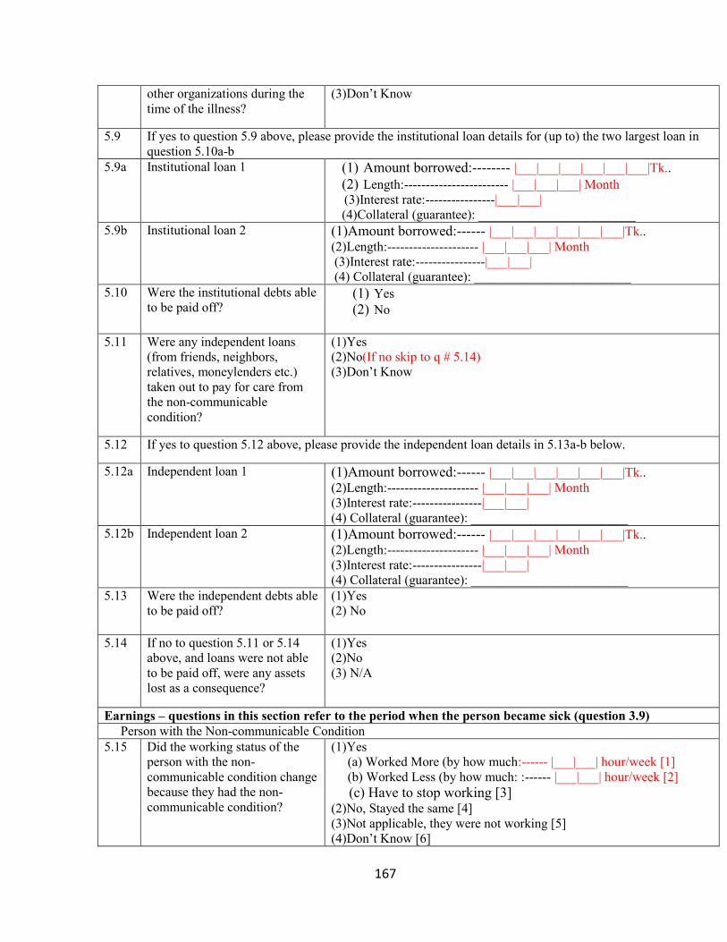
167
other organizations during the
time of the illness? (3)Don’t Know
5.9 If yes to question 5.9 above, please provide the institutional loan details for (up to) the two largest loan in
question 5.10a-b 5.9a Institutional loan 1 (1) Amount borrowed:-------- |___|___|___|___|___|___|Tk..
(2) Length:------------------------ |___|___|___| Month (3)Interest rate:----------------|___|___| (4)Collateral (guarantee): ________________________
5.9b Institutional loan 2 (1)Amount borrowed:------ |___|___|___|___|___|___|Tk.. (2)Length:--------------------- |___|___|___| Month (3)Interest rate:----------------|___|___| (4) Collateral (guarantee): ________________________
5.10 Were the institutional debts able
to be paid off? (1) Yes (2) No
5.11 Were any independent loans
(from friends, neighbors,
relatives, moneylenders etc.)
taken out to pay for care from
the non-communicable
condition?
(1)Yes (2)No(If no skip to q # 5.14) (3)Don’t Know
5.12 If yes to question 5.12 above, please provide the independent loan details in 5.13a-b below.
5.12a Independent loan 1 (1)Amount borrowed:------ |___|___|___|___|___|___|Tk.. (2)Length:--------------------- |___|___|___| Month (3)Interest rate:----------------|___|___| (4) Collateral (guarantee): ________________________
5.12b Independent loan 2 (1)Amount borrowed:------ |___|___|___|___|___|___|Tk.. (2)Length:--------------------- |___|___|___| Month (3)Interest rate:----------------|___|___| (4) Collateral (guarantee): ________________________
5.13 Were the independent debts able
to be paid off? (1)Yes (2) No
5.14 If no to question 5.11 or 5.14
above, and loans were not able
to be paid off, were any assets
lost as a consequence?
(1)Yes (2)No (3) N/A
Earnings – questions in this section refer to the period when the person became sick (question 3.9) Person with the Non-communicable Condition 5.15 Did the working status of the
person with the non-
communicable condition change
because they had the non-
communicable condition?
(1)Yes (a) Worked More (by how much:------ |___|___| hour/week [1] (b) Worked Less (by how much: :------ |___|___| hour/week [2] (c) Have to stop working [3] (2)No, Stayed the same [4] (3)Not applicable, they were not working [5] (4)Don’t Know [6]

168
5.16 Was work absenteeism an issue
for the person with the non-
communicable condition person
because they had the condition?
(1)Yes (2) No (3)Don’t Know (4) Not applicable (not in working)
5.17 Did the earnings of the person
with the non-communicable
condition change while they
were still working, because they
had the condition?
(1)Yes (a) Increased (by how much:---------- |___|___|___|___|Tk./week (b) Decreased (by how much: ---------|___|___|___|___|Tk./week (2)No, Stayed the Same (3)Not applicable, they were not working (3)Don’t Know
Household Members 5.18 Did the working status of the
household members already in
the labor force change because
the person had the non-
communicable condition?
(1)Yes (a) Worked More (by how much :------ |___|___| Hour/week (b) Worked Less (by how much:------- |___|___| Hour/week (2)No, Stayed the same (3)Not applicable, they were not working (4)Don’t Know
5.19 Was work absenteeism an issue
for the household members
because the deceased person
had the condition?
(1)Yes (2) No (3)Not applicable,( they were not working) (4)Don’t Know
5.20 Did household members not
previously in the labor force
have to enter the labor force
because the person had the
condition?
(1)Yes (2) No (3)Don’t Know
5.21 If Yes to question 5.21 above,
did the person have to leave
school to enter the work force?
(1)Yes If yes specify the level) 00=None 01-09=Exact year (specify:____________) 10=S.S.C 12=H.S.C 14=B.A, B.Sc, B.Com 16=M.A, M.Sc, M.Com. (2) No (3) Not applicable( No school going member in HH) (4)Don’t Know
5.22 Did the earnings of the
household members already in
the labor force change because
the person had the condition?
(1)Yes (a) Increased (by how much:---------- |___|___|___|___|Tk./week (b) Decreased (by how much:--------- |___|___|___|___|Tk./week (2)No, Stayed the Same (3)Not applicable, they were not working (3)Don’t Know
5.23 If a person had to stop working
while the person was sick with
the condition, were they able to
re-enter the workforce at a later
point?
(1)Yes (2) No (3) Don’t Know (4) Not applicable ( Nobody stop working)

169
Total Household 5.24 Did total household earnings
(person with non-communicable
condition and other household
members) change because the
person had the condition?
(1)Yes (a) Increased (by how much:------------ |___|___|___|___|Tk./week (b) Decreased (by how much:----------- |___|___|___|___|Tk./week (2)No, Stayed the Same (3)Not applicable, they were not working (4)Don’t Know
Remittances Received 5.25 Did the amount of remittances
received change during the time
when the person had the illness
mainly due to the illness?
(1)Yes (a) Increased (by how much:------------- |___|___|___|___|Tk./Month (b) Decreased (by how much:------------ |___|___|___|___|Tk./Month (2)No, Stayed the Same (3)Not applicable, none received (4)Don’t Know
Government Transfers 5.26 Did income received from any
public or government transfers
(i.e. the social safety net
programs, SSNP) change during
the time of the illness, mainly
due to the illness?
(1)Yes (a) Increased (by how much:----------- |___|___|___|___|Tk./Month (b) Decreased (by how much: ----------|___|___|___|___|Tk./Month (2)No, Stayed the Same (3)Not applicable, none received (4)Don’t Know
Family Arrangements & Education 5.27 Did family members have to
move out of the house, during
the time of the illness of the
person who died, mainly due to
the illness?
(1)Yes (2)No (3)Don’t Know
5.28 Did family members have to
move into the house, during the
time of the illness of the person
who died, mainly due to the
illness?
(1)Yes (2)No (3)Don’t Know
5.29 Did any members of the
household marry early or marry
underage (ages 0-18) or delay
marriage, during the time of the
illness, mainly as a result of the
economic impact due to the
illness of the person who died?
(1)Yes (check all that apply) marry early-- 1 delay marriage -- 2 (2)No (3)Don’t Know
5.30 Did any household members
have to stop attending school to
provide care for the person with
the condition during the time of
the illness of the person who
died?
(1)Yes ( If yes specify the level) 01-09=Exact year (specify:____________) 10=S.S.C 12=H.S.C 14=B.A, B.Sc, B.Com 16=M.A, M.Sc, M.Com. (2) No (3) Don’t Know

170
(4) Not applicable( No school going member in HH) 5.31 If a person had to stop education
during the time of the illness of
the person who died, were they
able to start again at a later
point?
(1)Yes (2)No (3)Don’t Know (4) N/A
5.32 Did any household members
attending school have worse
school performance during the
time of the illness due to the
illness of the person who died?
(1)Yes (2)No (3) Don’t Know (4) Not applicable( No school going member in HH)
Part 6: Economic Impact AFTER Time with Non-communicable Disease
All Questions refer to the current period in the household after the family member died (reference
date in question 3.5) of a non-communicable disease (minimum one year). All monetary figures
should be in Taka.
Expenditures & Food Security 6.1 Did total household
expenditures per week on basic
items (food, utilities, etc.)
change after the person passed
away?
(1)Food:--------------------------------|___|___|___|___|___|Tk./week (2) Utilities:------------------------------|___|___|___|___|___| Tk./week (3) Rent:------------------------|___|___|___|___|___| Tk./week (4) Tobacco:-------------------------- |___|___|___|___|___| Tk./week (5) Cell phone:------------------------|___|___|___|___|___| Tk./week (6) Transportation:--------------------|___|___|___|___|___| Tk./week (7) Hospitalization /Outpatient/ Diagnostic Test -|___|___|___|___|___|
Tk./week (8)Medication:--------------------------|___|___|___|___|___| Tk./week (9) Others (specify):----------------|___|___|___|___|___| Tk./week (10) Don`t Know
6.2 Did total household
expenditures per week on basic
items (food, utilities, etc.)
change after the person passed
away?
(1)Yes (a) Increased (by how much:--------|___|___|___|___| Tk/week.) (b) Decreased (by how much :----- |___|___|___|___| Tk/week.) (2)No, Stayed the same (3)Don’t Know
6.3 Did total household
expenditures on discretionary
items (non-essential foods, cell
phone, etc.) per week change
after the person passed away?
(1)Yes (a) Increased (by how much: ----------|___|___|___|___|Tk./week (b) Decreased (by how much: ---------|___|___|___|___|Tk./week (2)No, Stayed the same (3)Don’t Know
6.4 If tobacco was consumed in the
household, did household
expenditure on tobacco products
change after the person passed
away?
(1)Yes (a) Increased (by how much: -----------|___|___|___|___|Tk./week (b) Decreased (by how much: ----------|___|___|___|___|Tk./week (2)No, Stayed the same (3) Not applicable( tobacco was not consumed) (4)Don’t Know
Assets Savings and Loans

171
6.5 Were household savings used to
provide for the household after
the person passed away?
(1)Yes (how much was used: -----------|___|___|___|___|___|___|Tk. (2)No (3)Don’t Know (4) Not applicable( No savings)
6.6 Were household assets sold to
provide for the household after
the person passed away?
(1)Yes (amount received from the sale: --|___|___|___|___|___|___|Tk.) (2) No
6.7 Were any institutional loans
taken out with banks, NGOs, or
other organizations after the
person passed away?
(1)Yes (2)No(If no skip to q # 6.10) (3)Don’t Know
6.8 If yes to question 6.7 above, please provide the institutional loan details in questions 6.8a-b 6.8a Institutional loan 1 (1)Amount borrowed:------ |___|___|___|___|___|___|Tk..
(2)Length:--------------------- |___|___|___| Month (3)Interest rate:----------------|___|___| (4) Collateral (guarantee): ________________________
6.8b Institutional loan 2 (1)Amount borrowed:------ |___|___|___|___|___|___|Tk.. (2)Length:--------------------- |___|___|___| Month (3)Interest rate:----------------|___|___| (4) Collateral (guarantee): ________________________
6.9 Were the institutional debts able
to be paid off? (1) Yes (2) No (3) Partially
6.10 Were any independent loans
(from friends, neighbors,
relatives, moneylenders, etc.)
taken out after the person passed
away?
(1)Yes (2)No(If no skip to q # 6.13) (3)Don’t Know
6.11 If yes to question 6.10 above, please provide the independent loan details in 6.11a-b below.
6.11a Independent loan 1 (1)Amount borrowed:------ |___|___|___|___|___|___|Tk.. (2)Length:--------------------- |___|___|___| Month (3)Interest rate:----------------|___|___| (4) Collateral (guarantee): ________________________
6.11b Independent loan 2 (1)Amount borrowed:------ |___|___|___|___|___|___|Tk.. (2)Length:--------------------- |___|___|___| Month (3)Interest rate:----------------|___|___| (4) Collateral (guarantee): ________________________
6.12 Were the independent debts able
to be paid off? (1)Yes (2) No
6.13 If no to question 6.7or 6.10
above, and loans were not able
to be paid off, were any assets
lost as a consequence?
(1)Yes (2)No (3) Not applicable
Earnings
Household Members

172
6.14 Did the working status of the
household members already in
the labor force change mainly
due to the death from the non-
communicable condition after
the person passed away?
(1)Yes (a) Worked More (by how much :------- |___|___| Hour/week [1] (b) Worked Less (by how much :------- |___|___| Hour/week [2] (c) Have to stop working [3] (2)No, Stayed the same [4] (3)Not applicable, they were not working [5] (4)Don’t Know [6]
6.15 Was work absenteeism an issue
for the household members
mainly due to the death from the
non-communicable condition
after the person passed away?
(1)Yes (2) No (3) Not applicable, no member was working (4)Don’t Know
6.16 Did household members not
previously in the labor force
have to enter the labor force
mainly due to the death from the
non-communicable condition
after the person passed away?
(1)Yes (2) No -- Go to 6.18 (3)Don’t Know
6.17 If Yes to question 6.16 above,
did the person have to leave
school to enter the work force?
(1)Yes If yes specify the level) 01-09=Exact year (specify:____________) 10=S.S.C 12=H.S.C 14=B.A, B.Sc, B.Com 16=M.A, M.Sc, M.Com. (2) No (3)Don’t Know
6.18 Did the earnings of the
household members in the labor
force change mainly due to the
death from the non-
communicable condition after
the person passed away?
(1)Yes (a) Increased (by how much: ---------|___|___|___|___|Tk./week (b) Decreased (by how much: ---------|___|___|___|___|Tk./week (2)No, Stayed the Same (3)Don’t Know
Total Household 6.19 Did total household earnings
(all surviving household
members) change mainly due to
the death from the non-
communicable condition after
the person passed away?
(1)Yes (a) Increased (by how much: ---------|___|___|___|___|Tk./week (b) Decreased (by how much: ---------|___|___|___|___|Tk./week (2)No, Stayed the Same (3)Don’t Know
Remittances Received 6.20 Did the amount of remittances
received change mainly due to
the death from the non-
communicable condition after
the person passed away?
(1)Yes (a) Increased (by how much: ---------|___|___|___|___|Tk./Month (b) Decreased (by how much: ---------|___|___|___|___|Tk./Month (2)No, Stayed the Same (3)Not applicable, none received (4)Don’t Know
Government Transfers

173
6.21 Did income received from any
public or government transfers
(i.e. the social safety net
programs, SSNP) change
mainly due to the death from the
non-communicable condition
after the person passed away?
(1)Yes (a) Increased (by how much: ---------|___|___|___|___|Tk./Month (b) Decreased (by how much: ---------|___|___|___|___|Tk./Month (2)No, Stayed the Same (3)Not applicable, none received (4)Don’t Know
Family Arrangements & Education 6.22 Did family members have to
move out of the house, mainly
due to the death from the non-
communicable condition after
the person passed away?
(1)Yes (2)No (3)Don’t Know
6.23 Did family members have to
move into the house, mainly due
to the death from the non-
communicable condition after
the person passed away?
(1)Yes (2)No (3)Don’t Know
6.24 Did any members of the
household marry early or marry
underage (ages 0-18) or delay
marriage, mainly due to the
death from the non-
communicable condition after
the person passed away?
(1)Yes (check all that apply) marry early --1 delay marriage--2 (2)No (3)Don’t Know
6.25 Did any household members
have to stop attending school
mainly due to the death from the
non-communicable condition
after the person passed away?
(1) YES (If yes specify the level) 01-09=Exact year (specify:____________) 10=S.S.C 12=H.S.C 14=B.A, B.Sc, B.Com 16=M.A, M.Sc, M.Com. (2) No (3) Not applicable (no school going member) (4) Don’t Know
6.26 Did any household members
attending school have worse
school performance mainly due
to the death from the non-
communicable condition after
the person passed away?
(1)Yes (2)No (3) Not applicable (no school going member) (4) Don’t Know

174
Appendix B - Extra Tables for Chapter 2 Table B-1. (Corresponds to Table 2-2). OLS Regressions on the components of
Wealth, Marital Status and Occupation
Marital Status – Male
Marital Status – Female
Occupation – Male
Occupation – Female
Wealth – Male
Wealth - Female
Constant -0.171*** 0.447*** 0.932*** 0.097*** 1.694*** 1.341***
(0.006) (0.006) (0.005) (0.003) (0.016) (0.015)
Edu Year 0.007*** 0.008*** 0.010*** 0.016*** 0.110*** 0.154***
(0.000) (0.000) (0.000) (0.000) (0.001) (0.001)
Age 0.023*** 0.004*** -0.006*** -0.001*** -0.006*** 0.007***
(0.000) (0.000) (0.000) (0.000) (0.000) (0.000)
Muslim -0.005* 0.001 -0.100*** 0.003* 0.361*** 0.319***
(0.003) (0.003) (0.003) (0.002) (0.008) (0.008)
Household size -0.005*** 0.005*** 0.006*** -0.002*** 0.143*** 0.147***
(0.000) (0.000) (0.000) (0.000) (0.001) (0.001)
Cohort ages 40-59
-0.243*** -0.249*** 0.044*** 0.018*** 0.075*** 0.300***
(0.004) (0.004) (0.004) (0.002) (0.012) (0.011)
Cohort ages 60 and above
-1.012*** -0.721*** 0.106*** 0.033*** 0.590*** 0.315***
(0.007) (0.007) (0.007) (0.004) (0.021) (0.019)
Census 1996 0.089*** 0.126*** 0.069*** -0.029*** 0.087*** -0.085***
(0.003) (0.003) (0.002) (0.002) (0.007) (0.007)
Census 2005 0.135*** 0.175*** 0.109*** -0.039*** 0.104*** -0.190***
(0.003) (0.003) (0.002) (0.002) (0.007) (0.007)
R2 0.184 0.175 0.051 0.044 0.204 0.223
Num. obs. 186264 203266 170652 203266 186264 203266 ***p < 0.01, **p < 0.05, *p < 0.1
Table B-2 (Corresponds to Table 2-3 and 2-5) Cox Proportional Hazards Model on
Male NCD Mortality.
Unadjusted Adjusted Adjusted + Marital
Adjusted + Occ
Adjusted + Wealth
Adjusted + Marital + Occ + Wealth
Edu Year -0.019***
-0.021***
0.003 -0.017***
-0.011**
0.004
(0.005) (0.004) (0.004) (0.005) (0.005) (0.005)

175
Age 0.084***
0.068***
0.018***
0.067***
0.068***
0.018***
(0.001) (0.002) (0.002) (0.002) (0.002) (0.002)
Muslim (ref. Hindu) -0.210***
-0.218***
-0.159***
-0.234***
-0.188***
-0.154***
(0.043) (0.043) (0.044) (0.044) (0.043) (0.045)
Household size -0.021***
-0.016***
-0.001 -0.014**
-0.005 0.004
(0.006) (0.006) (0.006) (0.006) (0.006) (0.006)
Cohort ages 40-59 (ref 15-39)
0.679***
0.923***
0.776***
0.671***
0.937***
(0.082) (0.103) (0.087) (0.081) (0.103)
Cohort ages 60 and above (ref 15-39)
1.052***
1.109***
1.153***
1.056***
1.121***
(0.109) (0.128) (0.114) (0.109) (0.129)
Census 1996 (ref. 1982) 0.117***
0.828***
0.158***
0.120***
0.842***
(0.045) (0.046) (0.045) (0.045) (0.046)
Census 2005 (ref. 1982) 0.441***
2.465***
0.476***
0.440***
2.472***
(0.042) (0.047) (0.043) (0.042) (0.047)
Married (ref. Single/Never Married)
-5.115***
-5.087***
(0.464) (0.472)
Widow/Divorced (ref. Single/Never Married)
3.378***
3.401***
(0.126) (0.153)
student (ref. No Occupation)
-0.690**
-0.748**
(0.302) (0.322)
housework (ref. No Occupation)
0.389 1.277
(0.740) (0.905)
skilled agri (ref. No Occupation)
-0.611***
-0.559***
(0.069) (0.073)
elementary labor (ref. No Occupation)
-0.448***
-0.476***
(0.076) (0.079)
manufacture/skilled work/service (ref. No Occupation)
-0.608***
-0.484***
(0.078) (0.079)
business (ref. No Occupation)
-0.576***
-0.474***
(0.083) (0.085)
others (ref. No Occupation)
-0.441**
-0.386**
(0.180) (0.181)
Quintile 2 (ref. Quintile 1)
-0.155***
-0.067
(0.054) (0.054)

176
Quintile 3 (ref. Quintile 1)
-0.242***
-0.112**
(0.053) (0.053)
Quintile 4 (ref. Quintile 1)
-0.310***
-0.116**
(0.053) (0.053)
Quintile 5 (ref. Quintile 1)
-0.317***
-0.101*
(0.055) (0.056)
AIC 93457.023 93212.628 82336.758 93126.969 93177.684 82279.876
R2 0.052 0.053 0.107 0.053 0.053 0.107
Max. R2 0.426 0.426 0.426 0.426 0.426 0.426
Num. events 4317 4317 4317 4317 4317 4317
Num. obs. 186264 186264 186264 186264 186264 186264
PH test 0.512 0.000 0.000 0.000 0.000 0.000 ***
p < 0.01, **
p < 0.05, *p < 0.1
Table B-3 (Corresponds to Table 2-3 and 2-5) Cox Proportional Hazards Model on
Male Infectious Mortality.
Unadjusted Adjusted Adjusted + Marital
Adjusted + Occ
Adjusted + Wealth
Adjusted + Marital + Occ + Wealth
Edu Year -0.096***
-0.080***
-0.063***
-0.066***
-0.064***
-0.041***
(0.007) (0.007) (0.007) (0.007) (0.007) (0.007)
Age 0.076***
0.072***
0.049***
0.068***
0.074***
0.047***
(0.001) (0.003) (0.003) (0.003) (0.003) (0.003)
Muslim (ref. Hindu) -0.179***
-0.093* -0.111
** -0.137
** -0.043 -0.103
*
(0.057) (0.056) (0.056) (0.058) (0.056) (0.057)
Household size 0.012* -0.013
* -0.010 -0.012
* 0.009 0.009
(0.007) (0.007) (0.007) (0.007) (0.008) (0.008)
Cohort ages 40-59 (ref 15-39)
0.118 -0.295***
0.270***
0.087 -0.238**
(0.092) (0.112) (0.098) (0.092) (0.113)
Cohort ages 60 and above (ref 15-39)
0.333**
-0.300**
0.508***
0.315**
-0.218
(0.131) (0.145) (0.137) (0.131) (0.146)
Census 1996 (ref. 1982) -1.248***
-0.685***
-1.193***
-1.250***
-0.637***
(0.048) (0.050) (0.048) (0.048) (0.051)
Census 2005 (ref. 1982) -1.996***
-0.369***
-1.945***
-2.001***
-0.321***
(0.060) (0.070) (0.061) (0.060) (0.070)
Married (ref. Single/Never Married)
-4.096***
-3.978***
(0.333) (0.347)

177
Widow/Divorced (ref. Single/Never Married)
1.878***
2.001***
(0.140) (0.163)
student (ref. No Occupation)
0.036 -0.224
(0.248) (0.260)
housework (ref. No Occupation)
-11.418***
-11.027***
(0.178) (0.355)
skilled agri (ref. No Occupation)
-0.788***
-0.815***
(0.076) (0.073)
elementary labor (ref. No Occupation)
-0.452***
-0.582***
(0.083) (0.081)
manufacture/skilled work/service (ref. No Occupation)
-0.888***
-0.822***
(0.099) (0.095)
business (ref. No Occupation)
-0.854***
-0.836***
(0.110) (0.106)
others (ref. No Occupation)
-0.623***
-0.671***
(0.222) (0.233)
Quintile 2 (ref. Quintile 1)
-0.040 0.010
(0.066) (0.066)
Quintile 3 (ref. Quintile 1)
-0.357***
-0.279***
(0.069) (0.069)
Quintile 4 (ref. Quintile 1)
-0.383***
-0.275***
(0.068) (0.068)
Quintile 5 (ref. Quintile 1)
-0.526***
-0.392***
(0.072) (0.072)
AIC 53229.125 51675.298 48874.156 51527.793 51602.348 48702.968
R2 0.026 0.035 0.049 0.035 0.035 0.050
Max. R2 0.268 0.268 0.268 0.268 0.268 0.268
Num. events 2433 2433 2433 2433 2433 2433
Num. obs. 186264 186264 186264 186264 186264 186264
PH test 0.025 0.091 0.000 0.002 0.065 0.000 ***
p < 0.01, **
p < 0.05, *p < 0.1

178
Table B-4 (Corresponds to Table 2-3 and 2-4) Cox Proportional Hazards Model on
Female NCD Mortality.
Unadjusted Adjusted Adjusted + Marital
Adjusted + Occ
Adjusted + Wealth
Adjusted + Marital + Occ + Wealth
Edu Year -0.058***
-0.069***
-0.033***
-0.068***
-0.059***
-0.028**
(0.011) (0.011) (0.011) (0.011) (0.011) (0.012)
Age 0.092***
0.080***
0.064***
0.079***
0.081***
0.063***
(0.001) (0.002) (0.002) (0.002) (0.002) (0.002)
Muslim -0.253***
-0.253***
-0.218***
-0.252***
-0.236***
-0.209***
(0.050) (0.050) (0.049) (0.050) (0.050) (0.050)
Household size 0.005 0.012* 0.032
*** 0.011
* 0.019
*** 0.036
***
(0.006) (0.006) (0.006) (0.006) (0.007) (0.006)
Cohort ages 40-59 0.107 -0.531***
0.178* 0.122 -0.508
***
(0.090) (0.106) (0.092) (0.091) (0.106)
Cohort ages 60 and above
0.518***
-0.465***
0.595***
0.529***
-0.437***
(0.116) (0.129) (0.120) (0.116) (0.130)
Census 1996 -0.114**
0.155***
-0.087 -0.115**
0.180***
(0.054) (0.056) (0.054) (0.054) (0.056)
Census 2005 0.340***
0.897***
0.366***
0.338***
0.931***
(0.050) (0.055) (0.051) (0.050) (0.055)
Married -5.153***
-5.099***
(0.460) (0.465)
Widow/Divorced 0.971***
1.042***
(0.143) (0.159)
Student -0.029 -0.117
(0.295) (0.295)
Housework -0.331***
-0.432***
(0.097) (0.093)
Skilled agriculture -0.238 -0.467
(0.326) (0.324)
Elementary Labor -0.317* -0.649
***
(0.170) (0.167)
Manufacture/skilled work/service
-0.227 -0.463*
(0.260) (0.259)
Business -0.106 -0.223
(0.422) (0.419)
Others -0.569* -0.380
(0.330) (0.273)
Quintile 2 0.007 0.053
(0.060) (0.060)

179
Quintile 3 -0.013 0.060
(0.060) (0.060)
Quintile 4 -0.104* -0.019
(0.060) (0.061)
Quintile 5 -0.163**
-0.066
(0.064) (0.064)
AIC 67998.153 67833.796 65660.844 67821.011 67829.616 65653.375
R2 0.040 0.041 0.051 0.041 0.041 0.051
Max. R2 0.313 0.313 0.313 0.313 0.313 0.313
Num. events 3163 3163 3163 3163 3163 3163
Num. obs. 203266 203266 203266 203266 203266 203266
PH test 0.843 0.017 0.003 0.001 0.005 0.000 ***
p < 0.01, **
p < 0.05, *p < 0.1
Table B-5 (Corresponds to Table 2-3 and 2-4) Cox Proportional Hazards Model on
Female Infectious Mortality.
Unadjusted Adjusted Adjusted + Marital
Adjusted + Occ
Adjusted + Wealth
Adjusted + Marital + Occ + Wealth
Edu Year -0.212***
-0.128***
-0.108***
-0.129***
-0.114***
-0.094***
(0.018) (0.017) (0.017) (0.017) (0.017) (0.017)
Age 0.076***
0.080***
0.073***
0.076***
0.081***
0.069***
(0.002) (0.003) (0.003) (0.003) (0.003) (0.003)
Muslim -0.128**
-0.059 -0.054 -0.055 -0.026 -0.024
(0.062) (0.062) (0.062) (0.063) (0.062) (0.063)
Household size 0.039***
0.007 0.015**
0.007 0.022***
0.028***
(0.008) (0.007) (0.007) (0.007) (0.008) (0.008)
Cohort ages 40-59 -0.507***
-1.147***
-0.404***
-0.495***
-1.079***
(0.087) (0.090) (0.090) (0.087) (0.091)
Cohort ages 60 and above
-0.116 -0.895***
0.019 -0.110 -0.812***
(0.128) (0.125) (0.133) (0.128) (0.127)
Census 1996 -1.162***
-0.951***
-1.110***
-1.162***
-0.897***
(0.049) (0.050) (0.050) (0.049) (0.051)
Census 2005 -2.287***
-1.910***
-2.232***
-2.291***
-1.844***
(0.069) (0.073) (0.069) (0.069) (0.073)
Married -5.179***
-5.050***
(0.427) (0.430)
Widow/Divorced -0.171 -0.015
(0.152) (0.163)
Student
0.063 -0.112

180
(0.286) (0.270)
Housework -0.618***
-0.623***
(0.083) (0.080)
Skilled agriculture -1.328**
-1.396**
(0.604) (0.597)
Elementary Labor -0.450***
-0.683***
(0.173) (0.171)
Manufacture/skilled work/service
-1.018**
-1.185***
(0.461) (0.458)
Business -0.451 -0.512
(0.527) (0.528)
Others 0.029 0.028
(0.300) (0.281)
Quintile 2 -0.137* -0.095
(0.071) (0.071)
Quintile 3 -0.226***
-0.163**
(0.071) (0.071)
Quintile 4 -0.223***
-0.168**
(0.070) (0.070)
Quintile 5 -0.364***
-0.306***
(0.075) (0.075)
AIC 46774.889 45184.614 44167.070 45125.240 45169.862 44107.065
R2 0.023 0.030 0.035 0.031 0.030 0.036
Max. R2 0.224 0.224 0.224 0.224 0.224 0.224
Num. events 2131 2131 2131 2131 2131 2131
Num. obs. 203266 203266 203266 203266 203266 203266
PH test 0.046 0.112 0.174 0.164 0.049 0.137
***p < 0.01,
**p < 0.05,
*p < 0.1

181
Figure B-1.
Note: All models use Cox Proportional Hazard regression with censoring from death or outmigration for
the Matlab population in 1982, 1996 and 2005 (82-XX, 96-XX, 05-XX). The dependent variable, death, is
coded as binary. The independent variable for education is coded as having “no edu” and “edu” by
whether an individual had any years of formal education completed. 5 year follow up was used for years
1982 and 1996 and 4.5 years of follow up was used for 2005 due to data limitations.
Figure B-2
Note: All models use Cox Proportional Hazard regression with censoring from death or outmigration for
the Matlab population in 1982, 1996 and 2005 (82-XX, 96-XX, 05-XX). The dependent variable, death, is
coded as binary. The independent variable for education is coded as having “no edu” and “edu” by
whether an individual had any years of formal education completed. 5 year follow up was used for years
1982 and 1996 and 4.5 years of follow up was used for 2005 due to data limitations.

182
Figure B-3
Note: All models use Cox Proportional Hazard regression with censoring from death or outmigration for
the Matlab population in 1982, 1996 and 2005 (82-XX, 96-XX, 05-XX). The dependent variable, death, is
coded as binary. The independent variable for education is coded as having “no edu” and “edu” by
whether an individual had any years of formal education completed. 5 year follow up was used for years
1982 and 1996 and 4.5 years of follow up was used for 2005 due to data limitations.
Figure B-4
Note: All models use Cox Proportional Hazard regression with censoring from death or outmigration for
the Matlab population in 1982, 1996 and 2005 (82-XX, 96-XX, 05-XX). The dependent variable, death, is
coded as binary. The independent variable for education is coded as having “no edu” and “edu” by
whether an individual had any years of formal education completed. 5 year follow up was used for years
1982 and 1996 and 4.5 years of follow up was used for 2005 due to data limitations.

183
Appendix C – Extra Tables for Chapter 4 Table C-1. (Corresponding to Table 4-5) Logistic Regression Model for Coping Strategy for NCD death and Comparison
Group
Basic Exp Instit. Loan
Ind. Loan Spend Savings
Sell Assets Decrease SSN Transfer
Move Out Move In Marry Early
Leave Education
(Intercept) -2.493
(0.357)***
-0.704
(0.422)*
-1.626
(0.776)**
-1.213
(0.307)***
-2.544
(0.439)***
-4.396
(2.086)**
-2.170
(0.454)***
-4.745
(1.003)***
-4.300
(0.915)***
-1.459
(0.503)***
ncd 2.195
(0.115)***
-0.556
(0.164)***
-0.944
(0.369)**
-1.701
(0.136)***
-1.080
(0.187)***
2.162
(0.639)***
-1.335
(0.212)***
0.557
(0.281)**
0.161 (0.339)
-0.269 (0.196)
h_age_09 0.001 (0.004)
-0.027
(0.005)***
-0.032
(0.010)***
0.003 (0.004)
0.006 (0.005)
-0.045
(0.021)**
-0.009
(0.005)*
0.005 (0.010)
-0.015 (0.013)
-0.026
(0.006)***
h_sex_09 -0.015 (0.136)
-0.467
(0.193)**
-0.324 (0.380)
-0.006 (0.123)
-0.216 (0.188)
0.544 (0.520)
0.312
(0.170)*
0.496 (0.327)
-0.900
(0.546)*
-0.340 (0.233)
h_edu_any_09ind -0.036 (0.118)
-0.511
(0.149)***
-0.550
(0.281)**
0.077 (0.101)
0.064 (0.148)
-1.082
(0.532)**
0.160 (0.154)
0.321 (0.307)
0.434 (0.340)
-0.075 (0.185)
relig 0.141 (0.170)
-0.146 (0.195)
-0.363 (0.367)
0.102 (0.144)
-0.066 (0.199)
0.956 (1.055)
0.279 (0.234)
0.317 (0.477)
0.712 (0.607)
-0.128 (0.244)
hh_size_09 -0.029 (0.021)
0.063
(0.022)***
0.038 (0.062)
0.025 (0.017)
0.032 (0.022)
-0.036 (0.086)
0.012 (0.027)
-0.001 (0.049)
0.050 (0.049)
0.039 (0.029)
pov_sr 0.083 (0.117)
0.527
(0.150)***
0.491
(0.295)*
0.029 (0.100)
-0.008 (0.148)
0.520 (0.527)
0.344
(0.152)**
-0.679
(0.329)**
-0.153 (0.329)
0.414
(0.188)**
AIC 2085.743 1476.795 489.313 2597.793 1505.259 186.964 1394.172 508.592 399.722 1040.886
BIC 2132.367 1523.419 535.937 2644.417 1551.883 233.588 1440.796 555.216 446.346 1087.510
Log Likelihood -1034.871 -730.397 -236.656 -1290.896 -744.629 -85.482 -689.086 -246.296 -191.861 -512.443
Deviance 2069.743 1460.795 473.313 2581.793 1489.259 170.964 1378.172 492.592 383.722 1024.886
Num. obs. 2510 2510 2510 2510 2510 2510 2510 2510 2510 2510 ***
p < 0.01, **
p < 0.05, *p < 0.1
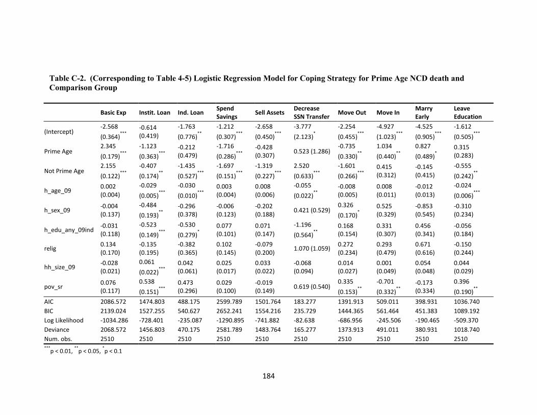
184
Table C-2. (Corresponding to Table 4-5) Logistic Regression Model for Coping Strategy for Prime Age NCD death and
Comparison Group
Basic Exp Instit. Loan Ind. Loan Spend Savings
Sell Assets Decrease SSN Transfer
Move Out Move In Marry Early
Leave Education
(Intercept) -2.568
(0.364)***
-0.614 (0.419)
-1.763
(0.776)**
-1.212
(0.307)***
-2.658
(0.450)***
-3.777
(2.123)*
-2.254
(0.455)***
-4.927
(1.023)***
-4.525
(0.905)***
-1.612
(0.505)***
Prime Age 2.345
(0.179)***
-1.123
(0.363)***
-0.212 (0.479)
-1.716
(0.286)***
-0.428 (0.307)
0.523 (1.286) -0.735
(0.330)**
1.034
(0.440)**
0.827
(0.489)*
0.315 (0.283)
Not Prime Age 2.155
(0.122)***
-0.407
(0.174)**
-1.435
(0.527)***
-1.697
(0.151)***
-1.319
(0.227)***
2.520
(0.633)***
-1.601
(0.266)***
0.415 (0.312)
-0.145 (0.415)
-0.555
(0.242)**
h_age_09 0.002 (0.004)
-0.029
(0.005)***
-0.030
(0.010)***
0.003 (0.004)
0.008 (0.006)
-0.055
(0.022)**
-0.008 (0.005)
0.008 (0.011)
-0.012 (0.013)
-0.024
(0.006)***
h_sex_09 -0.004 (0.137)
-0.484
(0.193)**
-0.296 (0.378)
-0.006 (0.123)
-0.202 (0.188)
0.421 (0.529) 0.326
(0.170)*
0.525 (0.329)
-0.853 (0.545)
-0.310 (0.234)
h_edu_any_09ind -0.031 (0.118)
-0.523
(0.149)***
-0.530
(0.279)*
0.077 (0.101)
0.071 (0.147)
-1.196
(0.564)**
0.168 (0.154)
0.331 (0.307)
0.456 (0.341)
-0.056 (0.184)
relig 0.134 (0.170)
-0.135 (0.195)
-0.382 (0.365)
0.102 (0.145)
-0.079 (0.200)
1.070 (1.059) 0.272 (0.234)
0.293 (0.479)
0.671 (0.616)
-0.150 (0.244)
hh_size_09 -0.028 (0.021)
0.061
(0.022)***
0.042 (0.061)
0.025 (0.017)
0.033 (0.022)
-0.068 (0.094)
0.014 (0.027)
0.001 (0.049)
0.054 (0.048)
0.044 (0.029)
pov_sr 0.076 (0.117)
0.538
(0.151)***
0.473 (0.296)
0.029 (0.100)
-0.019 (0.149)
0.619 (0.540) 0.335
(0.153)**
-0.701
(0.332)**
-0.173 (0.334)
0.396
(0.190)**
AIC 2086.572 1474.803 488.175 2599.789 1501.764 183.277 1391.913 509.011 398.931 1036.740
BIC 2139.024 1527.255 540.627 2652.241 1554.216 235.729 1444.365 561.464 451.383 1089.192
Log Likelihood -1034.286 -728.401 -235.087 -1290.895 -741.882 -82.638 -686.956 -245.506 -190.465 -509.370
Deviance 2068.572 1456.803 470.175 2581.789 1483.764 165.277 1373.913 491.011 380.931 1018.740
Num. obs. 2510 2510 2510 2510 2510 2510 2510 2510 2510 2510 ***
p < 0.01, **
p < 0.05, *p < 0.1

185
Table C-3. (Corresponding to Table 4-5) Logistic Regression Model for Coping Strategy for Head of Household NCD death
and Comparison Group
Basic Exp Instit. Loan Ind. Loan Spend Savings
Sell Assets Decrease SSN Transfer
Move Out Move In Marry Early
Leave Education
(Intercept) -2.619
(0.378)***
-0.702
(0.424)*
-1.548
(0.771)**
-1.219
(0.310)***
-2.681
(0.457)***
-4.914
(2.111)**
-2.061
(0.459)***
-4.706
(1.045)***
-4.273
(1.026)***
-1.297
(0.522)**
Head 2.136
(0.129)***
-0.552
(0.198)***
-0.754
(0.449)*
-1.713
(0.164)***
-1.324
(0.245)***
1.740
(0.730)**
-1.067
(0.240)***
0.585
(0.330)*
0.185 (0.400)
-0.052 (0.232)
Not Head 2.321
(0.162)***
-0.562
(0.243)**
-1.246
(0.601)**
-1.675
(0.227)***
-0.654
(0.280)**
2.524
(0.743)***
-1.947
(0.433)***
0.503 (0.405)
0.118 (0.564)
-0.648
(0.331)*
h_age_09 0.004 (0.005)
-0.027
(0.005)***
-0.033
(0.010)***
0.003 (0.004)
0.009 (0.006)
-0.033 (0.023)
-0.011
(0.005)**
0.004 (0.011)
-0.016 (0.014)
-0.029
(0.007)***
h_sex_09 -0.039 (0.139)
-0.466
(0.194)**
-0.307 (0.380)
-0.007 (0.123)
-0.241 (0.189)
0.395 (0.591) 0.336
(0.171)**
0.504 (0.321)
-0.895 (0.550)
-0.306 (0.233)
h_edu_any_09ind -0.041 (0.119)
-0.511
(0.148)***
-0.546
(0.279)*
0.077 (0.101)
0.060 (0.148)
-1.104
(0.535)**
0.166 (0.154)
0.322 (0.307)
0.435 (0.341)
-0.067 (0.185)
relig 0.140 (0.170)
-0.146 (0.195)
-0.363 (0.367)
0.102 (0.144)
-0.070 (0.200)
0.961 (1.051) 0.282 (0.234)
0.318 (0.476)
0.712 (0.608)
-0.128 (0.243)
hh_size_09 -0.032 (0.021)
0.063
(0.022)***
0.040 (0.062)
0.025 (0.017)
0.030 (0.022)
-0.057 (0.097)
0.015 (0.027)
0.000 (0.050)
0.051 (0.048)
0.044 (0.029)
pov_sr 0.084 (0.117)
0.527
(0.150)***
0.491
(0.295)*
0.029 (0.100)
-0.007 (0.148)
0.536 (0.528) 0.343
(0.152)**
-0.679
(0.330)**
-0.153 (0.329)
0.413
(0.188)**
AIC 2086.566 1478.794 490.846 2599.774 1503.858 187.563 1392.374 510.564 401.710 1040.253
BIC 2139.018 1531.246 543.298 2652.226 1556.310 240.016 1444.826 563.017 454.162 1092.705
Log Likelihood -1034.283 -730.397 -236.423 -1290.887 -742.929 -84.782 -687.187 -246.282 -191.855 -511.126
Deviance 2068.566 1460.794 472.846 2581.774 1485.858 169.563 1374.374 492.564 383.710 1022.253
Num. obs. 2510 2510 2510 2510 2510 2510 2510 2510 2510 2510 ***
p < 0.01, **
p < 0.05, *p < 0.1

186
Table C-4. (Corresponding to Table 4-5) Logistic Regression Model for Coping Strategy for Male or Female Household NCD
death and Comparison Group
Basic Exp Instit. Loan Ind. Loan Spend Savings
Sell Assets Decrease SSN Transfer
Move Out Move In Marry Early
Leave Education
(Intercept) -2.460
(0.358)***
-0.727
(0.420)*
-1.581
(0.780)**
-1.212
(0.307)***
-2.556
(0.441)***
-4.620
(2.053)**
-2.144
(0.454)***
-4.679
(1.011)***
-4.500
(0.925)***
-1.394
(0.501)***
fem_death 2.103
(0.140)***
-0.443
(0.216)**
-1.334
(0.603)**
-1.721
(0.199)***
-0.971
(0.262)***
2.704
(0.650)***
-1.840
(0.371)***
0.187 (0.396)
0.589 (0.431)
-0.579
(0.294)**
male_death 2.267
(0.133)***
-0.663
(0.216)***
-0.674 (0.440)
-1.685
(0.176)***
-1.168
(0.251)***
0.907 (0.915)
-1.016
(0.248)***
0.805
(0.330)**
-0.318 (0.493)
-0.047 (0.232)
h_age_09 0.000 (0.004)
-0.027
(0.005)***
-0.033
(0.010)***
0.003 (0.004)
0.006 (0.005)
-0.040
(0.020)**
-0.010
(0.005)*
0.004 (0.010)
-0.011 (0.013)
-0.027
(0.006)***
h_sex_09 0.021 (0.139)
-0.482
(0.192)**
-0.296 (0.382)
-0.004 (0.124)
-0.228 (0.190)
0.250 (0.547) 0.347
(0.173)**
0.591
(0.334)*
-0.987
(0.557)*
-0.302 (0.238)
h_edu_any_09ind -0.037 (0.118)
-0.513
(0.149)***
-0.546
(0.279)*
0.077 (0.101)
0.064 (0.148)
-1.085
(0.538)**
0.160 (0.154)
0.310 (0.307)
0.430 (0.340)
-0.071 (0.185)
relig 0.135 (0.170)
-0.143 (0.194)
-0.370 (0.367)
0.102 (0.144)
-0.066 (0.200)
1.086 (1.062) 0.275 (0.234)
0.303 (0.479)
0.733 (0.608)
-0.137 (0.244)
hh_size_09 -0.028 (0.021)
0.062
(0.022)***
0.039 (0.062)
0.025 (0.017)
0.031 (0.022)
-0.055 (0.088)
0.014 (0.027)
0.002 (0.049)
0.043 (0.050)
0.042 (0.029)
pov_sr 0.083 (0.117)
0.528
(0.150)***
0.490
(0.295)*
0.029 (0.100)
-0.008 (0.148)
0.577 (0.524) 0.345
(0.152)**
-0.678
(0.330)**
-0.151 (0.329)
0.413
(0.189)**
AIC 2086.487 1478.199 490.421 2599.774 1506.933 181.666 1392.208 508.647 399.138 1040.474
BIC 2138.939 1530.651 542.874 2652.226 1559.386 234.118 1444.660 561.099 451.591 1092.926
Log Likelihood -1034.243 -730.099 -236.211 -1290.887 -744.467 -81.833 -687.104 -245.324 -190.569 -511.237
Deviance 2068.487 1460.199 472.421 2581.774 1488.933 163.666 1374.208 490.647 381.138 1022.474
Num. obs. 2510 2510 2510 2510 2510 2510 2510 2510 2510 2510 ***
p < 0.01, **
p < 0.05, *p < 0.1

187
Table C-5. (Corresponding to Table 4-5) Logistic Regression Model for Coping Strategy for Long or Short Severe Morbidity
NCD death and Comparison Group
Basic Exp Instit. Loan Ind. Loan Spend Savings
Sell Assets Decrease SSN Transfer
Move Out Move In Marry Early
Leave Education
(Intercept) -2.485
(0.357)***
-0.697
(0.422)*
-1.598
(0.783)**
-1.212
(0.307)***
-2.540
(0.439)***
-4.416
(2.074)**
-2.169
(0.455)***
-4.751
(0.999)***
-4.301
(0.916)***
-1.451
(0.504)***
severe.long 2.373
(0.135)***
-0.384
(0.207)*
-0.435 (0.412)
-1.614
(0.183)***
-0.827
(0.233)***
2.033
(0.701)***
-1.265
(0.286)***
0.820
(0.325)**
0.208 (0.440)
-0.044 (0.241)
severe.short 2.027
(0.134)***
-0.737
(0.225)***
-1.821
(0.727)**
-1.788
(0.189)***
-1.381
(0.283)***
2.272
(0.688)***
-1.404
(0.293)***
0.233 (0.388)
0.116 (0.430)
-0.525
(0.277)*
h_age_09 0.001 (0.004)
-0.027
(0.005)***
-0.032
(0.010)***
0.003 (0.004)
0.006 (0.005)
-0.045
(0.021)**
-0.009
(0.005)*
0.005 (0.010)
-0.015 (0.013)
-0.026
(0.006)***
h_sex_09 -0.028 (0.137)
-0.475
(0.193)**
-0.347 (0.380)
-0.007 (0.123)
-0.221 (0.189)
0.566 (0.510) 0.310
(0.170)*
0.487 (0.328)
-0.902
(0.546)*
-0.352 (0.235)
h_edu_any_09ind -0.038 (0.119)
-0.514
(0.149)***
-0.561
(0.282)**
0.077 (0.101)
0.063 (0.148)
-1.077
(0.535)**
0.160 (0.154)
0.320 (0.308)
0.433 (0.341)
-0.080 (0.186)
relig 0.142 (0.171)
-0.145 (0.195)
-0.363 (0.367)
0.102 (0.144)
-0.066 (0.200)
0.956 (1.055) 0.279 (0.234)
0.318 (0.476)
0.713 (0.607)
-0.127 (0.245)
hh_size_09 -0.030 (0.021)
0.063
(0.022)***
0.037 (0.063)
0.025 (0.017)
0.032 (0.022)
-0.035 (0.085)
0.012 (0.027)
-0.001 (0.050)
0.050 (0.049)
0.039 (0.029)
pov_sr 0.084 (0.117)
0.529
(0.150)***
0.496
(0.292)*
0.029 (0.100)
-0.008 (0.148)
0.518 (0.530) 0.345
(0.152)**
-0.680
(0.329)**
-0.152 (0.330)
0.417
(0.188)**
AIC 2081.579 1477.206 487.723 2599.312 1504.672 188.775 1396.045 508.652 401.693 1040.785
BIC 2134.032 1529.658 540.176 2651.765 1557.124 241.227 1448.497 561.105 454.145 1093.237
Log Likelihood -1031.790 -729.603 -234.862 -1290.656 -743.336 -85.388 -689.023 -245.326 -191.846 -511.392
Deviance 2063.579 1459.206 469.723 2581.312 1486.672 170.775 1378.045 490.652 383.693 1022.785
Num. obs. 2510 2510 2510 2510 2510 2510 2510 2510 2510 2510 ***
p < 0.01, **
p < 0.05, *p < 0.1

188
Table C-6. (Corresponding to Table 4-5) Logistic Regression Model for Coping Strategy with Poor Interaction with NCD
death and Comparison Group
Basic Exp Instit. Loan Ind. Loan Spend Savings
Sell Assets Decrease SSN Transfer
Move Out Move In Marry Early
Leave Education
(Intercept) -2.406
(0.359)***
-0.680 (0.422)
-1.611
(0.762)**
-1.240
(0.309)***
-2.572
(0.440)***
-4.521
(2.059)**
-2.161
(0.453)***
-4.730
(1.010)***
-4.261
(0.898)***
-1.456
(0.501)***
ncd 2.030
(0.151)***
-0.704
(0.260)***
-1.102
(0.625)*
-1.472
(0.170)***
-0.881
(0.234)***
2.326
(1.107)**
-1.425
(0.313)***
0.515 (0.332)
0.020 (0.439)
-0.287 (0.291)
pov_sr -0.157 (0.190)
0.467
(0.169)***
0.449 (0.318)
0.110 (0.109)
0.074 (0.159)
0.728 (1.262) 0.321
(0.162)**
-0.751
(0.443)*
-0.291 (0.407)
0.405
(0.218)*
h_age_09 0.001 (0.004)
-0.027
(0.005)***
-0.032
(0.010)***
0.003 (0.004)
0.006 (0.005)
-0.045
(0.021)**
-0.009
(0.005)*
0.005 (0.010)
-0.015 (0.013)
-0.026
(0.006)***
h_sex_09 -0.014 (0.137)
-0.466
(0.193)**
-0.323 (0.380)
-0.007 (0.123)
-0.218 (0.188)
0.545 (0.520) 0.312
(0.170)*
0.497 (0.327)
-0.898 (0.546)
-0.340 (0.233)
h_edu_any_09ind -0.029 (0.118)
-0.507
(0.149)***
-0.547
(0.281)*
0.072 (0.101)
0.059 (0.148)
-1.085
(0.524)**
0.162 (0.154)
0.323 (0.310)
0.441 (0.348)
-0.074 (0.186)
relig 0.142 (0.171)
-0.145 (0.194)
-0.362 (0.367)
0.103 (0.145)
-0.065 (0.200)
0.951 (1.061) 0.279 (0.234)
0.317 (0.477)
0.714 (0.607)
-0.128 (0.244)
hh_size_09 -0.029 (0.021)
0.063
(0.022)***
0.038 (0.062)
0.025 (0.017)
0.032 (0.022)
-0.036 (0.086)
0.012 (0.027)
-0.001 (0.049)
0.050 (0.048)
0.039 (0.029)
ncd:pov_sr 0.380 (0.233)
0.251 (0.334)
0.252 (0.786)
-0.576
(0.286)**
-0.510 (0.395)
-0.255 (1.356)
0.172 (0.426)
0.153 (0.639)
0.369 (0.713)
0.032 (0.395)
AIC 2085.055 1478.222 491.206 2595.588 1505.516 188.928 1396.007 510.533 401.445 1042.879
BIC 2137.507 1530.675 543.658 2648.041 1557.968 241.380 1448.459 562.986 453.897 1095.331
Log Likelihood -1033.527 -730.111 -236.603 -1288.794 -743.758 -85.464 -689.003 -246.267 -191.722 -512.439
Deviance 2067.055 1460.222 473.206 2577.588 1487.516 170.928 1378.007 492.533 383.445 1024.879
Num. obs. 2510 2510 2510 2510 2510 2510 2510 2510 2510 2510 ***
p < 0.01, **
p < 0.05, *p < 0.1

189
Appendix D - Curriculum Vitae EDUCATION AND TRAINING
1. UNIVERSITY OF VIRGINIA Degree: Bachelor of Science in Biomedical Engineering, Minor in Spanish Literature Year: 2006
2. JOHNS HOPKINS BLOOMBERG SCHOOL OF PUBLIC HEALTH Degree: Master of Public Health, Concentration in Comparative Health Systems, Certificate in Health Economics Year: 2009 Capstone title: Evaluation of the decision-making process for vaccine introduction in Peru
3. JOHNS HOPKINS BLOOMBERG SCHOOL OF PUBLIC HEALTH Department: International Health, Health Systems Program Degree: PhD, Certificate in Demographic Methods Year: 2014 (expected summer graduation) Dissertation title: The economic impacts of adult non-communicable disease mortality for households in rural Bangladesh Advisor: Antonio J. Trujillo
PROFESSIONAL EXPERIENCE 2014 – Present Harvard Medical School, Cambridge, MA
Collaborate with a professor of Biostatistics in the Health Care Policy Department to develop analytical methods for matched cohort studies.
2009 – 2010 Research Associate, University of East Anglia, Norwich, UK
Developed probabilistic life table model to estimate chronic disease and risk factor burden and prevention cost-effectiveness in China
Major contributions to the analysis and writing of the final report: “Toward a Healthy and Harmonious Life in China: Stemming the Rising Tide of Non-Communicable Diseases.” World Bank Press, July 2011.
Summer 2009 Intern, The Stimson Center, Washington, DC
Work on Global Trends 2030 report commissioned by the NSA.
Conducted expert interviews and contributed to chapters on the topics of biotechnology and climate change.
2006 – 2008 Project Manager, Washington Occupational Health Associates, Washington, DC
Management of cancer screening program large US chemical company.
Review of client policy for pandemic flu preparedness.
PROFESSIONAL ACTIVITIES Society Membership
International Health Economics Association (iHEA)
Consultations The World Bank

190
Providing regression modeling support in STATA.
Westat/National Heart Lung Blood Institute (NHLBI)
Developed online training module for NHLBI fellows titled: “Introduction to Health Economics for Health Researchers.”
Save the Children USA (SC USA)
Developed a manual, “Introduction to Cost-Effective Analysis” for SC USA employees and worked updated cost estimates used for SC USA advocacy.
Center for Public Program Evaluation
Qualitative logic model evaluation of project for USA national public health organization.
EDITORIAL ACTIVITIES Peer Review Activities
Health Policy
PloS Medicine
PloS ONE
Journal of Health Population and Nutrition
Health Policy and Planning
PUBLICATIONS Journal Articles – Published peer reviewed 1. Ozawa, Sachiko; Mirelman, Andrew; Stack, Meghan L; Walker, Damian G; Levine, Orin S.
Cost-effectiveness and Economic Benefits of Vaccines in Low- and Middle- Income Countries: A Systematic Review. Vaccine Dec 2012; 31(1): 96-108.
2. Mirelman, Andrew; Mentzakis, Emmanouil; Kinter, Elizabeth; Paolucci, Francesco; Fordham, Richard; Ozawa, Sachiko; Ferraz, Marcos; Baltussen, Rob; Niessen, Louis W. Decision Making Criteria among National Policymakers in Five Countries: A Discrete Choice Experiment Eliciting Relative Preferences for Equity and Efficiency. Value in Health May 2012; 15(3): 534-539.
3. Defechereux, Thierry; Paolucci, Francesco; Mirelman, Andrew; Youngkong, Sitaporn; Botten, Grete; Hagen, Terje P; Niessen, Louis W. Health care priority setting in Norway a multicriteria decision analysis. BMC Health Services Research 2012. 12(39).
4. Curran, Kelly; Njeuhmeli, Emmanuel; Mirelman, Andrew; Dickson, Kim; Adamu, Tigistu; Cherutich, Peter; Mahler, Hally; Fimbo, Bennett; Mavuso, Thembisile Khumalo; Albertini, Jennifer. Voluntary Medical Male Circumcision: Strategies for Meeting the Human Resources Needs of Scale-Up in Southern and Eastern Africa. PLoS Medicine Nov 2011; 8(11): e1001129.
5. Stack, Meghan L; Ozawa, Sachiko; Bishai, David M; Mirelman, Andrew; Tam, Yvonne; Niessen, Louis; Walker, Damian G; Levine, Orin S. Estimated Economic Benefits During The ‘Decade Of Vaccines’ Include Treatment Savings, Gains In Labor Productivity. Health Affairs 2011; 30(6): 1021-1028.
6. Ozawa, Sachiko; Stack, Meghan L; Bishai, David M; Mirelman, Andrew; Friberg, Ingrid K; Niessen, Louis; Walker, Damian G; Levine, Orin S. During The ‘Decade Of Vaccines’, The Lives Of 6.4 Million Children Valued At $231 Billion Could Be Saved. Health Affairs 2011; 30(6): 1010-1020.
7. Boyette, Lisa B; Reardon, Michael A; Mirelman, Andrew J; Kirkley, Terry D; Lysiak, Jeffrey J; Tuttle, Jeremy B; Steers, William D. Fiber Optic Imaging of Cavernous Nerve In Vitro. The Journal of Urology 2007; 178(6): 2694-2700.
191
Journal Articles – In Press, Accepted for publication, Submitted for publication 1. Mirelman, Andrew; Grewal, Simrun; Ozawa Sachiko. The benefits and challenges for new
childhood vaccines in BRICS countries. Accepted for publication. Bulletin WHO. 2. Liang, Lilin; Mirelman, Andrew; The Impacts of Government Size, Indebtedness and Polity
on Government Health Expenditure: A Cross-Country Analyses over 1995-2010. Accepted for publication. Social Science and Medicine.
3. Khan, Jahangir AM; Trujillo, Antonio J; Ahmed, Sayem; Siddiquee, Ali T; Alam, N; Mirelman, Andrew; Koehlmoos, Tracey P; Niessen, Louis W; Peters, David H. Distribution of Non-Communicable Disease Mortality and Deterioration in Socioeconomic Status in Rural Bangladesh. Working Paper.
4. Cárdenas, María K; Galvin, Cooper; Mirelman, Andrew; Lazo, María; Pinto, Miguel; Miranda, J. Jaime; Gilman, Robert H. The cost of illness attributable to diabetic foot and cost-effectiveness of secondary prevention in Peru. Working Paper.
Journal Articles and Editorials – Not peer reviewed 1. Hospedales, James; Malekzadeh, Reza; Godoy, Daniela; Mirelman, Andrew; Boffetta,
Paolo. Improving National and Subnational Surveillance Data: The Models of Bangladesh, Iran and Chile, and the Role of PAHO. In Press. Scientific American.
2. Mirelman, Andrew; Koehlmoos, Tracey P; Niessen, Louis W. Risk-Attributable Burden of Chronic Diseases and Cost of Prevention in Bangladesh. Global Heart March 2012; 7(1): 61-66.
Reports, Manuals and Technical Guidelines 1. Institute of Medicine. Country-Level Decision Making for Control of Chronic Diseases:
Workshop Summary. 2012. Washington, DC; The National Academies Press. 2. Constenla, Dagna; Mirelman, Andrew; Alvaro, Arielle; Chen, A; Socal, M. The Economic
Value of Vaccines and Immunization Programs in Low- and Middle-Income Countries: An Annotated Bibliography. International Vaccine Access Center (IVAC), August 2012.
TEACHING Classroom Instruction 2013 – 2014: Johns Hopkins School of Public Health
1. Applications in Managing Health Organizations in Low and Middle Income Countries. Lecture – Developing a Health System Budget. Faculty: David Peters
2. Pharmaceutical Management in Low and Middle Income Countries. Lecture – The Cost-Effectiveness of Multi-dose combination therapy. Faculty: Maria Eng, Alan Lyles, David Peters.
2012 – 2013: Johns Hopkins School of Public Health 1. Summary Measures in Population Health. Lecture – Disease Modeling for National
Burden of Disease Estimates. Faculty: Adnan Hyder, Richard Morrow 2. Economic Evaluation II. Lecture – Incorporating Equity into Cost-Effectiveness Analysis.
Faculty: Dagna Constenla 3. Comparative Evaluation of Public Health Policies. Lecture – Equity and Efficiency
tradeoffs when measuring preferences for health policy. Faculty: Louis Niessen.

192
Teaching Assistantships 2013-2014: Johns Hopkins School of Public Health
1. Applications in Managing Health Organizations in Low and Middle Income Countries. Faculty: David Peters.
2012-2013: Johns Hopkins School of Public Health 1. Applications in Managing Health Organizations in Low and Middle Income Countries.
Faculty: David Peters. 2. Economic Evaluation III. Faculty: Louis Niessen, John Bridges. 3. Pharmaceutical Management in Low and Middle Income Countries. Faculty: Maria Eng,
Alan Lyles, David Peters 2011-2012: Johns Hopkins School of Public Health
1. Applications in Managing Health Organizations in Low and Middle Income Countries. Faculty: David Peters.
2. Economic Evaluation III. Faculty: Louis Niessen, John Bridges. 3. Comparative Evaluation of Public Health Interventions in Low and Middle Income
Countries. Faculty: Louis Niessen. 4. Health Economics I. Faculty: Kevin Frick.
2010-2011: Johns Hopkins School of Public Health 1. Applications in Managing Health Organizations in Low and Middle Income Countries.
Faculty: David Peters. 2. Understanding Cost-Effectiveness Analysis (online). Faculty: Kevin Frick. 3. Economic Evaluation II. Faculty: Amnesty LeFevre, Krishna Rao.
2009-2010: Johns Hopkins School of Public Health 1. Concepts and Application in Economic Evaluation I and II. Faculty: Damian Walker 2. Introduction to Health Systems in Low and Middle Income Countries. Faculty: Hafizur
Rahman. 3. Understanding Cost-Effectiveness Analysis (online). Faculty: Kevin Frick. 4. Statistical Reasoning in Public Health. Faculty: John McGready.
Other Significant Teaching 1. March 2011: Instructor, International Center for Diarrhoeal Disease Research (icddr,b),
Introduction to Modeling Concepts for Cost-Effectiveness Analysis
RESEARCH GRANT PARTICIPATION Title: Collaborating Centers of Excellence for Chronic Disease PI: David Peters. Year: 2011-2014 Source: United Health and the National Heart Lung Blood Institute Role: Research Assistant Title: Decade of Vaccines Economics Research PI: Sachiko Ozawa. Year: 2010-2014 Source: The Bill and Melinda Gates Foundation Role: Research Assistant
PRESENTATIONS Scientific Meetings

193
A cost-effectiveness analysis of human and pig vaccination strategies to reduce the burden of Japanese encephalitis in Bangladesh. American Society of Tropical Medicine and Hygiene (ASTMH). Poster Presentation. Washington DC. Nov. 13-17, 2013.
The impacts of non-communicable disease deaths on household wealth in rural Bangladesh. International Health Economics Association (iHEA). Biennial Conference. Sydney Conference Center; Sydney, Australia. June 20, 2013.
Developing a Price Tag for NCD Prevention: Example Country Case Studies from NHLBI Centers of Excellence. Workshop on Country-Level Decision Making for Control of Chronic Diseases. IOM House of Sweden; Washington, DC. July 19-21, 2011.
Invited Seminars “The impacts of non-communicable disease deaths on household wealth in rural
Bangladesh.” University of Washington Department of Global Health, June 20, 2013.
“A cost-effectiveness analysis of vaccination strategies to reduce the burden of Japanese encephalitis in Bangladesh”. JHSPH Health Economics Seminar, April 2013.