the econometrics of uncertainty shocks - sas.upenn.edujesusfv/lecture_4_ucl.pdf · tjt and s tjt 1,...
TRANSCRIPT

The Econometrics of Uncertainty Shocks
Jesús Fernández-Villaverde
University of Pennsylvania
March 7, 2016
Jesús Fernández-Villaverde (PENN) Econometrics March 7, 2016 1 / 69

Several challenges
Several challenges
How do we document the presence of time-varying uncertainty?
How do we distinguish time-variation in the data and in expectations?Forecaster disagreement?
How much of the uncertainty is exogenous or endogenous?
How do we take DSGE models with time-varying uncertainty to thedata?
1 Likelihood function.
2 Method of moments.
Because of time limitations, I will focus on the first and lastchallenges.
Jesús Fernández-Villaverde (PENN) Econometrics March 7, 2016 2 / 69

Documenting time-varying uncertainty.
Interest rates
Jesús Fernández-Villaverde (PENN) Econometrics March 7, 2016 3 / 69

Documenting time-varying uncertainty.
A real life example
Remember our decomposition of interest rates:
rt = r︸︷︷︸mean
+ εtb,t︸︷︷︸T-Bill shocks
+ εr ,t︸︷︷︸Spread shocks
εtb,t and εr ,t follow:
εtb,t = ρtbεtb,t−1 + eσtb,tutb,t , utb,t ∼ N (0, 1)
εr ,t = ρr εr ,t−1 + eσr ,tur ,t , ur ,t ∼ N (0, 1)
σtb,t and σr ,t follow:
σtb,t =(1− ρσtb
)σtb + ρσtb
σtb,t−1 + ηtbuσtb ,t , uσtb ,t ∼ N (0, 1)
σr ,t =(1− ρσr
)σr + ρσr
σr ,t−1 + ηruσr ,t , uσr ,t ∼ N (0, 1)
Jesús Fernández-Villaverde (PENN) Econometrics March 7, 2016 4 / 69

Documenting time-varying uncertainty.
Stochastic volatility
Remember, as well, that we postulated a general process forstochastic volatility:
xt = ρxt−1 + σt εt , εt ∼ N (0, 1).
and
log σt = (1− ρσ) log σ+ ρσ log σt−1 +(1− ρ2σ
) 12 ηut , ut ∼ N (0, 1).
We discussed this was a concrete example of a richer class ofspecifications.
Main point: non-linear structure.
Jesús Fernández-Villaverde (PENN) Econometrics March 7, 2016 5 / 69
Documenting time-varying uncertainty.
State space representation I
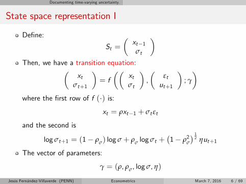
Define:
St =(xt−1σt
)Then, we have a transition equation:(
xtσt+1
)= f
((xtσt
),
(εtut+1
);γ
)where the first row of f (·) is:
xt = ρxt−1 + σt εt
and the second is
log σt+1 = (1− ρσ) log σ+ ρσ log σt +(1− ρ2σ
) 12 ηut+1
The vector of parameters:
γ = (ρ, ρσ, log σ, η)
Jesús Fernández-Villaverde (PENN) Econometrics March 7, 2016 6 / 69
Documenting time-varying uncertainty.
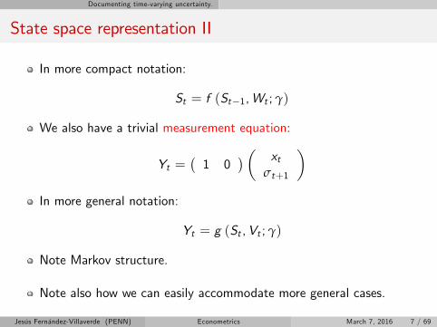
State space representation II
In more compact notation:
St = f (St−1,Wt ;γ)
We also have a trivial measurement equation:
Yt =(1 0
) ( xtσt+1
)In more general notation:
Yt = g (St ,Vt ;γ)
Note Markov structure.
Note also how we can easily accommodate more general cases.
Jesús Fernández-Villaverde (PENN) Econometrics March 7, 2016 7 / 69

Documenting time-varying uncertainty.
Shocks
{Wt} and {Vt} are independent of each other.
{Wt} is known as process noise and {Vt} as measurement noise.
Wt and Vt have zero mean.
No assumptions on the distribution beyond that.
Jesús Fernández-Villaverde (PENN) Econometrics March 7, 2016 8 / 69

Documenting time-varying uncertainty.
Conditional densities
From St = f (St−1,Wt ;γ) , we can compute p (St |St−1;γ).
From Yt = g (St ,Vt ;γ), we can compute p (Yt |St ;γ) .
From St = f (St−1,Wt ;γ) and Yt = g (St ,Vt ;γ), we have:
Yt = g (f (St−1,Wt ;γ) ,Vt ;γ)
and hence we can compute p (Yt |St−1;γ).
Jesús Fernández-Villaverde (PENN) Econometrics March 7, 2016 9 / 69

Filtering
Filtering, smoothing, and forecasting
Filtering: we are concerned with what we have learned up to currentobservation.
Smoothing: we are concerned with what we learn with the full sample.
Forecasting: we are concerned with future realizations.
Jesús Fernández-Villaverde (PENN) Econometrics March 7, 2016 10 / 69
Filtering
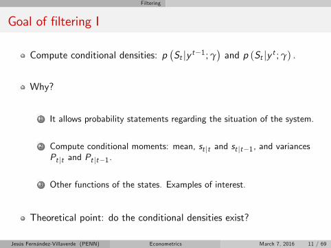
Goal of filtering I
Compute conditional densities: p(St |y t−1;γ
)and p (St |y t ;γ) .
Why?
1 It allows probability statements regarding the situation of the system.
2 Compute conditional moments: mean, st |t and st |t−1, and variancesPt |t and Pt |t−1.
3 Other functions of the states. Examples of interest.
Theoretical point: do the conditional densities exist?
Jesús Fernández-Villaverde (PENN) Econometrics March 7, 2016 11 / 69

Filtering
Goals of filtering II
Evaluate the likelihood function of the observables yT at parametervalues γ:
p(yT ;γ
)Given the Markov structure of our state space representation:
p(yT ;γ
)= p (y1|γ)
T
∏t=2p(yt |y t−1;γ
)Then:
p(yT ;γ
)=∫p (y1|s1;γ) dS1
T
∏t=2
∫p (yt |St ;γ) p
(St |y t−1;γ
)dSt
Hence, knowledge of{p(St |y t−1;γ
)}Tt=1 and p (S1;γ) allow the
evaluation of the likelihood of the model.
Jesús Fernández-Villaverde (PENN) Econometrics March 7, 2016 12 / 69
Filtering
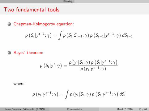
Two fundamental tools
1 Chapman-Kolmogorov equation:
p(St |y t−1;γ
)=∫p (St |St−1;γ) p
(St−1|y t−1;γ
)dSt−1
2 Bayes’theorem:
p(St |y t ;γ
)=p (yt |St ;γ) p
(St |y t−1;γ
)p (yt |y t−1;γ)
where:
p(yt |y t−1;γ
)=∫p (yt |St ;γ) p
(St |y t−1;γ
)dSt
Jesús Fernández-Villaverde (PENN) Econometrics March 7, 2016 13 / 69
Filtering
Interpretation
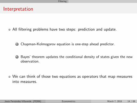
All filtering problems have two steps: prediction and update.
1 Chapman-Kolmogorov equation is one-step ahead predictor.
2 Bayes’theorem updates the conditional density of states given the newobservation.
We can think of those two equations as operators that map measuresinto measures.
Jesús Fernández-Villaverde (PENN) Econometrics March 7, 2016 14 / 69
Filtering
Recursion for conditional distribution
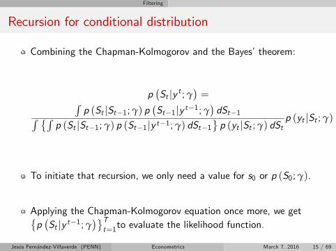
Combining the Chapman-Kolmogorov and the Bayes’theorem:
p(St |y t ;γ
)=∫
p (St |St−1;γ) p(St−1|y t−1;γ
)dSt−1∫ {∫
p (St |St−1;γ) p (St−1|y t−1;γ) dSt−1}p (yt |St ;γ) dSt
p (yt |St ;γ)
To initiate that recursion, we only need a value for s0 or p (S0;γ).
Applying the Chapman-Kolmogorov equation once more, we get{p(St |y t−1;γ
)}Tt=1to evaluate the likelihood function.
Jesús Fernández-Villaverde (PENN) Econometrics March 7, 2016 15 / 69

Filtering
Initial conditions
From previous discussion, we know that we need a value for s1 orp (S1;γ) .
Stationary models: ergodic distribution.
Non-stationary models: more complicated. Importance oftransformations.
Forgetting conditions.
Non-contraction properties of the Bayes operator.
Jesús Fernández-Villaverde (PENN) Econometrics March 7, 2016 16 / 69

Filtering
Smoothing
We are interested on the distribution of the state conditional on allthe observations, on p
(St |yT ;γ
)and p
(yt |yT ;γ
).
We compute:
p(St |yT ;γ
)= p
(St |y t ;γ
) ∫ p(St+1|yT ;γ
)p (St+1|St ;γ)
p (St+1|y t ;γ)dSt+1
a backward recursion that we initialize with p(ST |yT ;γ
),
{p (St |y t ;γ)}Tt=1 and{p(St |y t−1;γ
)}Tt=1 we obtained from filtering.
Jesús Fernández-Villaverde (PENN) Econometrics March 7, 2016 17 / 69
Filtering
Forecasting
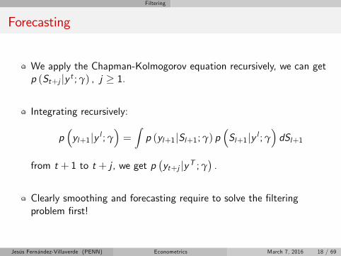
We apply the Chapman-Kolmogorov equation recursively, we can getp (St+j |y t ;γ) , j ≥ 1.
Integrating recursively:
p(yl+1|y l ;γ
)=∫p (yl+1|Sl+1;γ) p
(Sl+1|y l ;γ
)dSl+1
from t + 1 to t + j , we get p(yt+j |yT ;γ
).
Clearly smoothing and forecasting require to solve the filteringproblem first!
Jesús Fernández-Villaverde (PENN) Econometrics March 7, 2016 18 / 69
Filtering
Problem of filtering
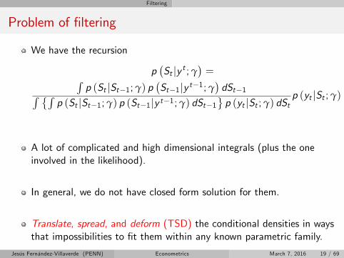
We have the recursion
p(St |y t ;γ
)=∫
p (St |St−1;γ) p(St−1|y t−1;γ
)dSt−1∫ {∫
p (St |St−1;γ) p (St−1|y t−1;γ) dSt−1}p (yt |St ;γ) dSt
p (yt |St ;γ)
A lot of complicated and high dimensional integrals (plus the oneinvolved in the likelihood).
In general, we do not have closed form solution for them.
Translate, spread, and deform (TSD) the conditional densities in waysthat impossibilities to fit them within any known parametric family.
Jesús Fernández-Villaverde (PENN) Econometrics March 7, 2016 19 / 69
Filtering
Exception
There is one exception: linear and Gaussian case.
Why? Because if the system is linear and Gaussian, all the conditionalprobabilities are also Gaussian.
Linear and Gaussian state spaces models translate and spread theconditional distributions, but they do not deform them.
For Gaussian distributions, we only need to track mean and variance(suffi cient statistics).
Kalman filter accomplishes this goal effi ciently.
Jesús Fernández-Villaverde (PENN) Econometrics March 7, 2016 20 / 69

Nonlinear Filtering
Nonlinear filtering
Different approaches.
Deterministic filtering:
1 Kalman family.
2 Grid-based filtering.
Simulation filtering:
1 McMc.
2 Particle filtering.
Jesús Fernández-Villaverde (PENN) Econometrics March 7, 2016 21 / 69

Nonlinear Filtering
Particle filtering I
Remember,
1 Transition equation:
St = f (St−1,Wt ;γ)
2 Measurement equation:
Yt = g (St ,Vt ;γ)
Jesús Fernández-Villaverde (PENN) Econometrics March 7, 2016 22 / 69

Nonlinear Filtering
Particle filtering II
Some Assumptions:
1 We can partition {Wt} into two independent sequences {W1,t} and{W2,t}, s.t. Wt = (W1,t ,W2,t ) anddim (W2,t ) + dim (Vt ) ≥ dim (Yt ).
2 We can always evaluate the conditional densitiesp(yt |W t
1 , yt−1, S0;γ
).
3 The model assigns positive probability to the data.
Jesús Fernández-Villaverde (PENN) Econometrics March 7, 2016 23 / 69

Nonlinear Filtering
Rewriting the likelihood function
Evaluate the likelihood function of the a sequence of realizations ofthe observable yT at a particular parameter value γ:
p(yT ;γ
)
We factorize it as (careful with initial condition!):
p(yT ;γ
)=
T
∏t=1p(yt |y t−1;γ
)=
T
∏t=1
∫ ∫p(yt |W t
1 , yt−1,S0;γ
)p(W t1 , S0|y t−1;γ
)dW t
1 dS0
Jesús Fernández-Villaverde (PENN) Econometrics March 7, 2016 24 / 69

Nonlinear Filtering
A law of large numbers
If{{st |t−1,i0 ,w t |t−1,i1
}Ni=1
}Tt=1
N i.i.d. draws from{p(W t1 , S0|y t−1;γ
)}Tt=1, then:
p(yT ;γ
)'
T
∏t=1
1N
N
∑i=1p(yt |w t |t−1,i1 , y t−1, st |t−1,i0 ;γ
)
The problem of evaluating the likelihood is equivalent to the problem ofdrawing from
{p(W t1 , S0|y t−1;γ
)}Tt=1
Jesús Fernández-Villaverde (PENN) Econometrics March 7, 2016 25 / 69

Nonlinear Filtering
Introducing particles I
{st−1,i0 ,w t−1,i1
}Ni=1
N i.i.d. draws from p(W t−11 ,S0|y t−1;γ
).
Each st−1,i0 ,w t−1,i1 is a particle and{st−1,i0 ,w t−1,i1
}Ni=1
a swarm of
particles.{st |t−1,i0 ,w t |t−1,i1
}Ni=1
N i.i.d. draws from p(W t1 ,S0|y t−1;γ
).
Jesús Fernández-Villaverde (PENN) Econometrics March 7, 2016 26 / 69
Nonlinear Filtering
Introducing particles II
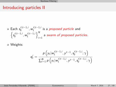
Each st |t−1,i0 ,w t |t−1,i1 is a proposed particle and{st |t−1,i0 ,w t |t−1,i1
}Ni=1
a swarm of proposed particles.
Weights:
qit =p(yt |w t |t−1,i1 , y t−1, st |t−1,i0 ;γ
)∑Ni=1 p
(yt |w t |t−1,i1 , y t−1, st |t−1,i0 ;γ
)
Jesús Fernández-Villaverde (PENN) Econometrics March 7, 2016 27 / 69
Nonlinear Filtering
A proposition
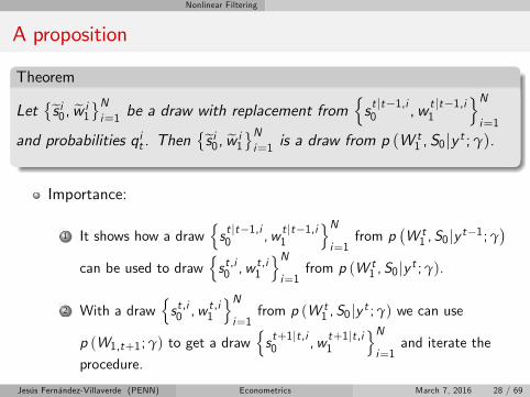
Theorem
Let{s̃ i0, w̃
i1
}Ni=1 be a draw with replacement from
{st |t−1,i0 ,w t |t−1,i1
}Ni=1
and probabilities qit . Then{s̃ i0, w̃
i1
}Ni=1 is a draw from p (W t
1 , S0|y t ;γ).
Importance:
1 It shows how a draw{st |t−1,i0 ,w t |t−1,i1
}Ni=1
from p(W t1 , S0 |y t−1;γ
)can be used to draw
{st ,i0 ,w
t ,i1
}Ni=1
from p (W t1 , S0 |y t ;γ).
2 With a draw{st ,i0 ,w
t ,i1
}Ni=1
from p (W t1 , S0 |y t ;γ) we can use
p (W1,t+1;γ) to get a draw{st+1|t ,i0 ,w t+1|t ,i1
}Ni=1
and iterate the
procedure.
Jesús Fernández-Villaverde (PENN) Econometrics March 7, 2016 28 / 69

Nonlinear Filtering
Algorithm
Step 0, Initialization: Set t 1 and setp(W t−11 ,S0|y t−1;γ
)= p (S0;γ).
Step 1, Prediction: Sample N values{st |t−1,i0 ,w t |t−1,i1
}Ni=1
from
the density p(W t1 ,S0|y t−1;γ
)= p (W1,t ;γ) p
(W t−11 , S0|y t−1;γ
).
Step 2, Weighting: Assign to each draw st |t−1,i0 ,w t |t−1,i1 theweight qit.
Step 3, Sampling: Draw{st ,i0 ,w
t ,i1
}Ni=1
with rep. from{st |t−1,i0 ,w t |t−1,i1
}Ni=1
with probabilities{qit}Ni=1. If t < T set
t t + 1 and go to step 1. Otherwise go to step 4.
Step 4, Likelihood: Use{{st |t−1,i0 ,w t |t−1,i1
}Ni=1
}Tt=1
to compute:
p(yT ;γ
)'
T
∏t=1
1N
N
∑i=1p(yt |w t |t−1,i1 , y t−1, st |t−1,i0 ;γ
)Jesús Fernández-Villaverde (PENN) Econometrics March 7, 2016 29 / 69

Nonlinear Filtering
Evaluating a Particle filter
We just saw a plain vanilla particle filter.
How well does it work in real life?
Is it feasible to implement in large models?
Jesús Fernández-Villaverde (PENN) Econometrics March 7, 2016 30 / 69

Nonlinear Filtering
Why did we resample?
We could have not resampled and just used the weights as you wouldhave done in importance sampling (this is known as sequentialimportance sampling).
Most weights go to zero.
But resampling impoverish the swarm.
Eventually, this becomes a problem.
Jesús Fernández-Villaverde (PENN) Econometrics March 7, 2016 31 / 69

Nonlinear Filtering
Jesús Fernández-Villaverde (PENN) Econometrics March 7, 2016 32 / 69

Nonlinear Filtering
Why did we resample?
Effective Sample Size:
ESSt =1[
∑Ni=1 p
(yt |w t |t−1,i1 , y t−1, st |t−1,i0 ;γ
)]2Alternatives:
1 Stratified resampling (Kitagawa, 1996): optimal in terms of variance.
2 Adaptive resampling.
Jesús Fernández-Villaverde (PENN) Econometrics March 7, 2016 33 / 69
Nonlinear Filtering
Simpler notation
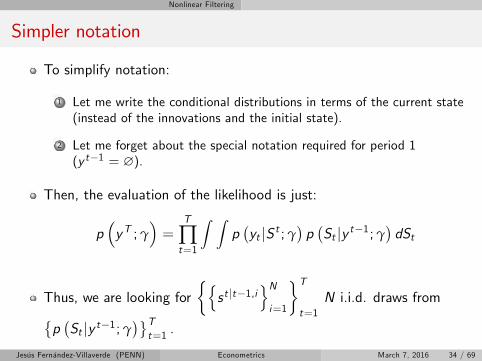
To simplify notation:
1 Let me write the conditional distributions in terms of the current state(instead of the innovations and the initial state).
2 Let me forget about the special notation required for period 1(y t−1 = ∅).
Then, the evaluation of the likelihood is just:
p(yT ;γ
)=
T
∏t=1
∫ ∫p(yt |S t ;γ
)p(St |y t−1;γ
)dSt
Thus, we are looking for{{st |t−1,i
}Ni=1
}Tt=1
N i.i.d. draws from{p(St |y t−1;γ
)}Tt=1 .
Jesús Fernández-Villaverde (PENN) Econometrics March 7, 2016 34 / 69
Nonlinear Filtering
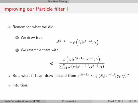
Improving our Particle filter I
Remember what we did:
1 We draw fromst |t−1,i ∼ p
(St |st−1,i ;γ
)2 We resample them with:
qit =p(yt |st |t−1,i , y t−1;γ
)∑Ni=1 p
(yt |st |t−1,i , y t−1;γ
)But, what if I can draw instead from st |t−1,i ∼ q
(St |st−1,i , yt ;γ
)?
Intuition.
Jesús Fernández-Villaverde (PENN) Econometrics March 7, 2016 35 / 69
Nonlinear Filtering
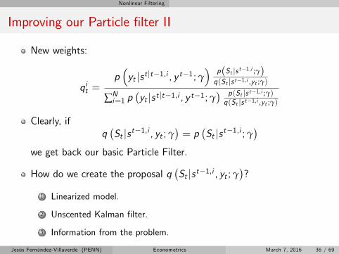
Improving our Particle filter II
New weights:
qit =p(yt |st |t−1,i , y t−1;γ
)p(St |s t−1,i ;γ)q(St |s t−1,i ,yt ;γ)
∑Ni=1 p
(yt |st |t−1,i , y t−1;γ
) p(St |s t−1,i ;γ)q(St |s t−1,i ,yt ;γ)
Clearly, ifq(St |st−1,i , yt ;γ
)= p
(St |st−1,i ;γ
)we get back our basic Particle Filter.
How do we create the proposal q(St |st−1,i , yt ;γ
)?
1 Linearized model.
2 Unscented Kalman filter.
3 Information from the problem.
Jesús Fernández-Villaverde (PENN) Econometrics March 7, 2016 36 / 69

Nonlinear Filtering
Improving our Particle filter III
Auxiliary Particle Filter: Pitt and Shephard (1999).
Imagine we can compute either
p(yt+1|st ,i
)or
p̃(yt+1|st ,i
)Then:
qit =p̃(yt+1|st ,i
)p(yt |st |t−1,i , y t−1;γ
)p(St |s t−1,i ;γ)q(St |s t−1,i ,yt ;γ)
∑Ni=1 p̃ (yt+1|st ,i ) p
(yt |st |t−1,i , y t−1;γ
) p(St |s t−1,i ;γ)q(St |s t−1,i ,yt ;γ)
Auxiliary Particle Filter tends to work well when we have fat tail...
...but it can temperamental.
Jesús Fernández-Villaverde (PENN) Econometrics March 7, 2016 37 / 69

Nonlinear Filtering
Improving our Particle filter IV
Resample-Move.
Blocking.
Many others.
A Tutorial on Particle Filtering and Smoothing: Fifteen years later, byDoucet and Johansen (2012)
Jesús Fernández-Villaverde (PENN) Econometrics March 7, 2016 38 / 69

Nonlinear Filtering
Nesting it in a McMc
Fernández-Villaverde and Rubio Ramírez (2007) and Flury andShepard (2008).
You nest the Particle filter inside an otherwise standard McMc.
Two caveats:
1 Lack of differentiability of the Particle filter.
2 Random numbers constant to avoid chatter and to be able to swapoperators.
Jesús Fernández-Villaverde (PENN) Econometrics March 7, 2016 39 / 69

Nonlinear Filtering
Parallel programming
Why?
Divide and conquer.
Shared and distributed memory.
Main approaches:
1 OpenMP.
2 MPI.
3 GPU programming: CUDA and OpenCL.
Jesús Fernández-Villaverde (PENN) Econometrics March 7, 2016 40 / 69

Nonlinear Filtering
Jesús Fernández-Villaverde (PENN) Econometrics March 7, 2016 41 / 69

Nonlinear Filtering
Tools
In Matlab: parallel toolboox.
In R: package parallel.
In Julia: built-in procedures.
In Mathematica: parallel computing tools.
GPUs: ArrayFire.
Jesús Fernández-Villaverde (PENN) Econometrics March 7, 2016 42 / 69

Nonlinear Filtering
Parallel Particle filter
Simplest strategy: generating and evaluating draws.
A temptation: multiple swarms.
How to nest with a McMc?
Jesús Fernández-Villaverde (PENN) Econometrics March 7, 2016 43 / 69
Nonlinear Filtering
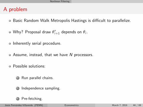
A problem
Basic Random Walk Metropolis Hastings is diffi cult to parallelize.
Why? Proposal draw θ∗i+1 depends on θi .
Inherently serial procedure.
Assume, instead, that we have N processors.
Possible solutions:
1 Run parallel chains.
2 Independence sampling.
3 Pre-fetching.
Jesús Fernández-Villaverde (PENN) Econometrics March 7, 2016 44 / 69

Nonlinear Filtering
Multiple chains
We run N chains, one in each processor.
We merge them at the end.
It goes against the principle of one, large chain.
But it may works well when the burn-in period is small.
If the burn-in is large or the chain has subtle convergence issues, itresults in waste of time and bad performance.
Jesús Fernández-Villaverde (PENN) Econometrics March 7, 2016 45 / 69
Nonlinear Filtering
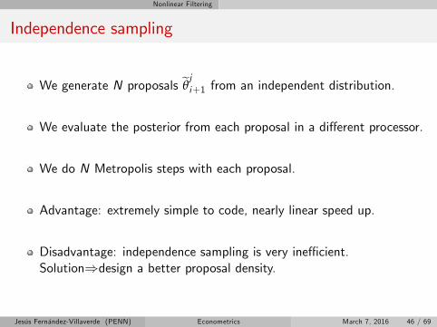
Independence sampling
We generate N proposals θ̃ji+1 from an independent distribution.
We evaluate the posterior from each proposal in a different processor.
We do N Metropolis steps with each proposal.
Advantage: extremely simple to code, nearly linear speed up.
Disadvantage: independence sampling is very ineffi cient.Solution⇒design a better proposal density.
Jesús Fernández-Villaverde (PENN) Econometrics March 7, 2016 46 / 69

Nonlinear Filtering
Prefetching I
Proposed by Brockwell (2006).
Idea: we can compute the relevant posteriors several periods inadvance.
Set superindex 1 for rejection and 2 for acceptance.
Advantage: if we reject a draw, we have already evaluated the nextstep.
Disadvantage: wasteful. More generally, you can show that the speedup will converge only to log2 N.
Jesús Fernández-Villaverde (PENN) Econometrics March 7, 2016 47 / 69

Nonlinear Filtering
Prefetching II
1 Assume we are at θi .
2 We draw 2 paths for iteration i + 1,{
θ̃1i+1 = θi , θ̃
2i+1 ∼ g (θi )
}.
3 We draw 4 paths for iteration i + 2{θ̃11i+2 = θ̃
1i+1, θ̃
12i+2 ∼ g
(θ̃1i+1
), θ̃21i+2 = θ̃
2i+1, θ̃
22i+2 ∼ g
(θ̃2i+1
)}.
4 We iterate h steps, until we have N = 2h possible sequences.
5 We evaluate each of the posteriors p(
θ̃1,...,1i+h
), ..., p
(θ̃2,...,2i+h
)in each
of the N processors.
6 We do a MH in each step of the path using the previous posteriors(note that any intermediate posterior is the same as the correspondingfinal draw where all the following children are “rejections”).
Jesús Fernández-Villaverde (PENN) Econometrics March 7, 2016 48 / 69

Nonlinear Filtering
A simpler prefetching algorithm I
Algorithm for N processors, where N is small.
Given θi :
1 We draw N{
θ̃i+1,1, ..., θ̃i+1,N
}and we evaluate the posteriors
p(
θ̃i+1,1
), ..., p
(θ̃i+1,N
).
2 We evaluate the first proposal, θ̃i+1,1:
1 If accepted, we disregard θi+1,2, ..., θi+1,2.
2 If rejected, we make θi+1 = θi and θ̃i+2,1 = θ̃i+1,2 is our new proposalfor i + 2.
3 We continue down the list of N proposals until we accept one.
Advantage: if we reject a draw, we have already evaluated the nextstep.
Jesús Fernández-Villaverde (PENN) Econometrics March 7, 2016 49 / 69

Nonlinear Filtering
A simpler prefetching algorithm II
Imagine we have a PC with N = 4 processors.
Well gauged acceptance for a normal SV model≈ 20%− 25%. Letme fix it to 25% for simplicity.
Then:
1 P(accepting 1st draw) = 0.25. We advance 1 step.
2 P(accepting 2nd draw) = 0.75 ∗ 0.25. We advance 2 steps.3 P(accepting 3tr draw) = 0.752 ∗ 0.25. We advance 3 steps.4 P(accepting 4th draw) = 0.753 ∗ 0.25. We advance 4 steps.5 P(not accepting any draw) = 0.75∗4. We advance 4 steps.
Therefore, expected numbers of steps advanced in the chain:
1 ∗ 0.25+ 2 ∗ 0.75 ∗ 0.25+ 3 ∗ 0.75∗2 ∗ 0.25+ 4 ∗ 0.753 = 2.7344Jesús Fernández-Villaverde (PENN) Econometrics March 7, 2016 50 / 69

Taking DSGE-SV Models to the Data
First-order approximation
Remember that the first-order approximation of a canonical RBCmodel without persistence in productivity shocks:
k̂t+1 = a1k̂t + a2εt , εt ∼ N (0, 1)
Then:
k̂t+1 = a1(a1k̂t−1 + a2εt−1
)+ a2εt
= a21 k̂t−1 + a1a2εt−1 + a2εt
Since a1 < 1 and assuming k̂0 = 0
k̂t+1 = a2t
∑j=0aj1εt−j
which is a well-understood MA system.
Jesús Fernández-Villaverde (PENN) Econometrics March 7, 2016 51 / 69

Taking DSGE-SV Models to the Data
Higher-order approximations
Second-order approximation:
k̂t+1 = a0 + a1k̂t + a2εt + a3k̂2t + a4ε2t + a5k̂t εt , εt ∼ N (0, 1)
Then:
k̂t+1 = a0 + a1(a0 + a1k̂t + a2εt + a3k̂2t + a4ε
2t + a5k̂t εt
)+ a2εt
+a3(a0 + a1k̂t + a2εt + a3k̂2t + a4ε
2t + a5k̂t εt
)2+ a4ε2t
+a5(a0 + a1k̂t + a2εt + a3k̂2t + a4ε
2t + a5k̂t εt
)εt
We have terms in k̂3t and k̂4t .
Jesús Fernández-Villaverde (PENN) Econometrics March 7, 2016 52 / 69
Taking DSGE-SV Models to the Data
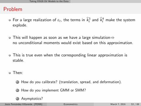
Problem
For a large realization of εt , the terms in k̂3t and k̂4t make the system
explode.
This will happen as soon as we have a large simulation⇒no unconditional moments would exist based on this approximation.
This is true even when the corresponding linear approximation isstable.
Then:
1 How do you calibrate? (translation, spread, and deformation).
2 How do you implement GMM or SMM?
3 Asymptotics?Jesús Fernández-Villaverde (PENN) Econometrics March 7, 2016 53 / 69

Taking DSGE-SV Models to the Data
A solution
For second-order approximations, Kim et al. (2008): pruning.
Idea:
k̂t+1 = a0 + a1(a0 + a1k̂t + a2εt + a3k̂2t + a4ε
2t + a5k̂t εt
)+ a2εt
+a3(a0 + a1k̂t + a2εt + a3k̂2t + a4ε
2t + a5k̂t εt
)2+ a4ε2t
+a5(a0 + a1k̂t + a2εt + a3k̂2t + a4ε
2t + a5k̂t εt
)εt
We omit terms raised to powers higher than 2.
Pruned approximation does not explode.
Jesús Fernández-Villaverde (PENN) Econometrics March 7, 2016 54 / 69

Taking DSGE-SV Models to the Data
What do we do?
Build a pruned state-space system.
Apply pruning to an approximation of any arbitrary order.
Prove that first and second unconditional moments exist.
Closed-form expressions for first and second unconditional momentsand IRFs.
Conditions for the existence of some higher unconditional moments,such as skewness and kurtosis.
Apply to a New Keynesian model with EZ preferences.
Software available for distribution.Jesús Fernández-Villaverde (PENN) Econometrics March 7, 2016 55 / 69
Taking DSGE-SV Models to the Data
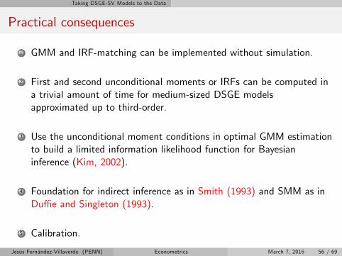
Practical consequences
1 GMM and IRF-matching can be implemented without simulation.
2 First and second unconditional moments or IRFs can be computed ina trivial amount of time for medium-sized DSGE modelsapproximated up to third-order.
3 Use the unconditional moment conditions in optimal GMM estimationto build a limited information likelihood function for Bayesianinference (Kim, 2002).
4 Foundation for indirect inference as in Smith (1993) and SMM as inDuffi e and Singleton (1993).
5 Calibration.
Jesús Fernández-Villaverde (PENN) Econometrics March 7, 2016 56 / 69

State-Space Representations
Dynamic models and state-space representations
Dynamic model:
xt+1 = h (xt , σ) + σηεt+1, εt+1 ∼ IID (0, I)yt = g (xt , σ)
Comparison with our previous structure.
Again, general framework (augmented state vector).
Jesús Fernández-Villaverde (PENN) Econometrics March 7, 2016 57 / 69
State-Space Representations
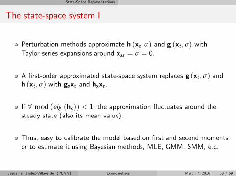
The state-space system I
Perturbation methods approximate h (xt , σ) and g (xt , σ) withTaylor-series expansions around xss = σ = 0.
A first-order approximated state-space system replaces g (xt , σ) andh (xt , σ) with gxxt and hxxt .
If ∀ mod (eig (hx)) < 1, the approximation fluctuates around thesteady state (also its mean value).
Thus, easy to calibrate the model based on first and second momentsor to estimate it using Bayesian methods, MLE, GMM, SMM, etc.
Jesús Fernández-Villaverde (PENN) Econometrics March 7, 2016 58 / 69

State-Space Representations
The state-space system II
We can replace g (xt , σ) and h (xt , σ) with their higher-orderTaylor-series expansions.
However, the approximated state-space system cannot, in general, beshown to have any finite moments.
Also, it often displays explosive dynamics.
This occurs even with simple versions of the New Keynesian model.
Hence, it is diffi cult to use the approximated state-space system tocalibrate or to estimate the parameters of the model.
Jesús Fernández-Villaverde (PENN) Econometrics March 7, 2016 59 / 69

State-Space Representations
The pruning method: second-order approximation I
Partition states: [ (xft)′
(xst )′]
Original state-space representation:
x(2)t+1 = hx(xft + x
st
)+12Hxx
((xft + x
st
)⊗(xft + x
st
))+12hσσσ2 + σηεt+1
y(2)t = gxx(2)t +
12Gxx
(x(2)t ⊗ x
(2)t
)+12gσσσ2
Jesús Fernández-Villaverde (PENN) Econometrics March 7, 2016 60 / 69
State-Space Representations
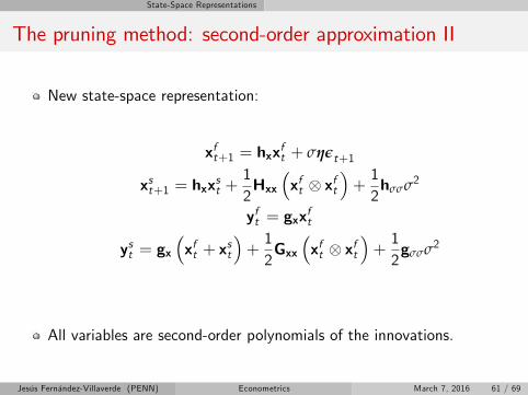
The pruning method: second-order approximation II
New state-space representation:
xft+1 = hxxft + σηεt+1
xst+1 = hxxst +
12Hxx
(xft ⊗ xft
)+12hσσσ2
yft = gxxft
yst = gx(xft + x
st
)+12Gxx
(xft ⊗ xft
)+12gσσσ2
All variables are second-order polynomials of the innovations.
Jesús Fernández-Villaverde (PENN) Econometrics March 7, 2016 61 / 69
State-Space Representations
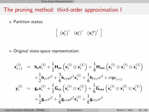
The pruning method: third-order approximation I
Partition states: [ (xft)′
(xst )′ (
xrdt)′ ]
Original state-space representation:
x(3)t+1 = hxx(3)t +
12Hxx
(x(3)t ⊗ x
(3)t
)+16Hxxx
(x(3)t ⊗ x
(3)t ⊗ x
(3)t
)+12hσσσ2 +
36hσσxσ
2x(3)t +16hσσσσ3 + σηεt+1
y(3)t = gxx(3)t +
12Gxx
(x(3)t ⊗ x
(3)t
)+16Gxxx
(x(3)t ⊗ x
(3)t ⊗ x
(3)t
)+12gσσσ2 +
36gσσxσ
2x(3)t +16gσσσσ3
Jesús Fernández-Villaverde (PENN) Econometrics March 7, 2016 62 / 69
State-Space Representations
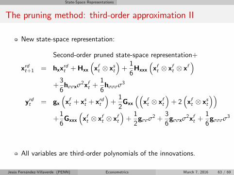
The pruning method: third-order approximation II
New state-space representation:
Second-order pruned state-space representation+
xrdt+1 = hxxrdt +Hxx(xft ⊗ xst
)+16Hxxx
(xft ⊗ xft ⊗ xf
)+36hσσxσ
2xft +16hσσσσ3
yrdt = gx(xft + x
st + x
rdt
)+12Gxx
((xft ⊗ xft
)+ 2
(xft ⊗ xst
))+16Gxxx
(xft ⊗ xft ⊗ xft
)+12gσσσ2 +
36gσσxσ
2xft +16gσσσσ3
All variables are third-order polynomials of the innovations.
Jesús Fernández-Villaverde (PENN) Econometrics March 7, 2016 63 / 69

State-Space Representations
Higher-order approximations
We can generalize previous steps:
1 Decompose the state variables into first-, second-, ... , and kth-ordereffects.
2 Set up laws of motions for the state variables capturing only first-,second-, ... , and kth-order effects.
3 Construct the expression for control variables by preserving onlyeffects up to kth-order.
Jesús Fernández-Villaverde (PENN) Econometrics March 7, 2016 64 / 69
State-Space Representations
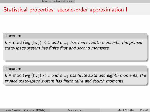
Statistical properties: second-order approximation I
Theorem
If ∀ mod (eig (hx)) < 1 and εt+1 has finite fourth moments, the prunedstate-space system has finite first and second moments.
Theorem
If ∀ mod (eig (hx)) < 1 and εt+1 has finite sixth and eighth moments, thepruned state-space system has finite third and fourth moments.
Jesús Fernández-Villaverde (PENN) Econometrics March 7, 2016 65 / 69
State-Space Representations
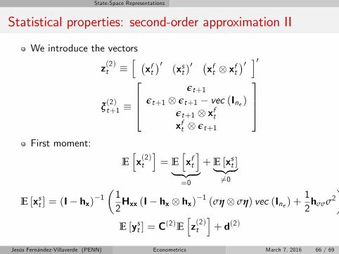
Statistical properties: second-order approximation II
We introduce the vectors
z(2)t ≡[ (xft)′
(xst )′ (
xft ⊗ xft)′ ]′
ξ(2)t+1 ≡
εt+1
εt+1 ⊗ εt+1 − vec (Ine )εt+1 ⊗ xftxft ⊗ εt+1
First moment:
E[x(2)t]= E
[xft]
︸ ︷︷ ︸=0
+E [xst ]︸ ︷︷ ︸6=0
E [xst ] = (I− hx)−1(12Hxx (I− hx ⊗ hx)−1 (ση⊗ ση) vec (Ine ) +
12hσσσ2
)E [yst ] = C
(2)E[z(2)t]+ d(2)
Jesús Fernández-Villaverde (PENN) Econometrics March 7, 2016 66 / 69
State-Space Representations
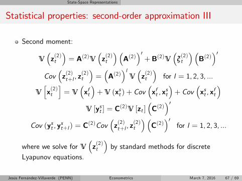
Statistical properties: second-order approximation III
Second moment:
V(z(2)t)= A(2)V
(z(2)t) (A(2)
)′+B(2)V
(ξ(2)t
) (B(2)
)′Cov
(z(2)t+l , z
(2)t
)=(A(2)
)lV(z(2)t)for l = 1, 2, 3, ...
V[x(2)t]= V
(xft)+V (xst ) + Cov
(xft , x
st
)+ Cov
(xst , x
ft
)V [yst ] = C
(2)V [zt ](C(2)
)′Cov (yst , y
st+l ) = C
(2)Cov(z(2)t+l , z
(2)t
) (C(2)
)′for l = 1, 2, 3, ...
where we solve for V(z(2)t)by standard methods for discrete
Lyapunov equations.
Jesús Fernández-Villaverde (PENN) Econometrics March 7, 2016 67 / 69

State-Space Representations
Statistical properties: second-order approximation IV
Generalized impulse response function (GIRF): Koop et al. (1996)
GIRFvar (l , ν,wt ) = E [vart+l |wt , εt+1 = ν]−E [vart+l |wt ]
Importance in models with volatility shocks.
Jesús Fernández-Villaverde (PENN) Econometrics March 7, 2016 68 / 69

State-Space Representations
Statistical properties: third-order approximation
Theorem
If ∀ mod (eig (hx)) < 1 and εt+1 has finite sixth moments, the prunedstate-space system has finite first and second moments.
Theorem
If ∀ mod (eig (hx)) < 1 and εt+1 has finite ninth and twelfth moments,the pruned state-space system has finite third and fourth moments.
Similar (but long!!!!!) formulae for first and second moments andIRFs.
Jesús Fernández-Villaverde (PENN) Econometrics March 7, 2016 69 / 69