Literature Review: Intelligent Robot Observers

Florian Shkurti

February 12, 2013

Contents

1 Introduction 1

2 Bayesian Filtering and Estimation 22.1 Bayesian Filtering . . . . . . . . . . . . . . . . . . . . . . . . . . . . . . . . . . . . . . . . 3

2.1.1 Kalman Filter . . . . . . . . . . . . . . . . . . . . . . . . . . . . . . . . . . . . . . . 32.1.2 Extended Kalman Filter . . . . . . . . . . . . . . . . . . . . . . . . . . . . . . . . . 42.1.3 Unscented Kalman Filter . . . . . . . . . . . . . . . . . . . . . . . . . . . . . . . . 5

2.2 Smoothing . . . . . . . . . . . . . . . . . . . . . . . . . . . . . . . . . . . . . . . . . . . . . 5

3 Sampling-based Path Planning 63.1 RRT . . . . . . . . . . . . . . . . . . . . . . . . . . . . . . . . . . . . . . . . . . . . . . . . 73.2 RRT* . . . . . . . . . . . . . . . . . . . . . . . . . . . . . . . . . . . . . . . . . . . . . . . 83.3 PRM . . . . . . . . . . . . . . . . . . . . . . . . . . . . . . . . . . . . . . . . . . . . . . . . 8

4 Clustering 104.1 k-means . . . . . . . . . . . . . . . . . . . . . . . . . . . . . . . . . . . . . . . . . . . . . . 114.2 Lloyd’s algorithm . . . . . . . . . . . . . . . . . . . . . . . . . . . . . . . . . . . . . . . . . 114.3 k-means++ . . . . . . . . . . . . . . . . . . . . . . . . . . . . . . . . . . . . . . . . . . . . 124.4 Maximum-likelihood clustering . . . . . . . . . . . . . . . . . . . . . . . . . . . . . . . . . 12

5 Classification and ensemble methods 135.1 Computing nearest neighbours . . . . . . . . . . . . . . . . . . . . . . . . . . . . . . . . . 135.2 Bagging classifiers . . . . . . . . . . . . . . . . . . . . . . . . . . . . . . . . . . . . . . . . 155.3 Boosting classifiers . . . . . . . . . . . . . . . . . . . . . . . . . . . . . . . . . . . . . . . . 15

6 Active Vision 166.1 Feature-level active vision . . . . . . . . . . . . . . . . . . . . . . . . . . . . . . . . . . . . 166.2 Image-level active vision . . . . . . . . . . . . . . . . . . . . . . . . . . . . . . . . . . . . . 176.3 Viewpoint-level active vision . . . . . . . . . . . . . . . . . . . . . . . . . . . . . . . . . . . 18

1 Introduction

Most of today’s robots collect video footage and other sensor data without being able to semanticallyinterpret what the data represents. This results in autonomous agents that do not have the ability todiscriminate which parts of the scene, or the sensor data, is informative and which is not, dependingon the robot’s surrounding environment and context. This literature review provides a summary ofalgorithms and important papers whose ideas can facilitate the design of an intelligent robot observer.

Ideally, such an observer would be able to discriminate between informative and non-informativeparts of a given scene, focusing its attention on events and places that are important and should berecorded, as opposed to recording everything. This active vision paradigm is one of the topics examinedin this review, and some of the key ideas are presented. Additionally, since robots have to process streamsof incoming data from multiple sources, preferably in real-time, methods that cluster, summarize, andcompress incoming data streams could be very beneficial towards this end. This motivated us to includea section on the analysis of clustering algorithms and their properties.

1

Classifying parts of the scene as important or not largely has to do with contextual information suchas the robot’s mission, its past experience, the surrounding parts of the scene etc. We therefore examinesome of the most well-known supervised classification methods, so that a number of basic learned rulesare incorporated in the decision-making process. For instance, such a rule might be to assign moreimportance to human activity than recording video of objects when both are present in the scene.

Navigating through the informative parts of the scene in the presence of dynamic obstacles is some-thing that we would like this type of observer to be capable of doing. To that end we summarize someof the most important path-planning algorithms that work without exhaustively modeling the availablespace that is obstacle-free. Some of these path-planners assume the existence of an accurate map andperfect localization within that map. In practice this is still a generally open problem in robotics, in thecase where the robot operates in unstructured environments. So, we dedicate a section of this review toestimation, localization and mapping methods, presenting some of the recent progress in this domain.

Sometimes this review focuses more on the algorithm properties and specific tools for each of theabove topics; this is because we believe that robotic systems should be accompanied by some theoreticaljustifications and analyses whenever possible, and not just deemed successful when they perform well ona restricted experimental scenario.

2 Bayesian Filtering and Estimation

Today’s robots rely on a variety of sensors and electro-mechanical actuators to measure properties oftheir environment (and themselves) and to affect it in some way. The range of available sensors is broad:

• Cameras that measure and digitize the intensity of light in the visible spectrum

• 2D or 3D laser rangefinders that return range and angle measurements to obstacles

• Inertial measurement units (IMUs) that measure angular velocity and linear acceleration

• GPS receivers based on trilateration of the receiver’s position with respect to orbiting satellites

• Infrared cameras that measure and digitize the intensity of light in the infrared spectrum

• SONAR sensors which can be used to measure distances based on the time-of-flight of emittedsound

• Tactile sensors, which measure contact forces

• Doppler Velocity Logs (DVLs) which measure the velocity of underwater vehicles and their distanceto the seafloor [1, p. 19-28]

• Underwater acoustic positioning systems, replicating GPS functionality underwater [1, p. 19-28]

• Rotary encoders, which measure the angle of a motor1

• Pressure sensors

• Altimeters

• Magnetic compasses

Although the list is seemingly long, it is only a short selection of sensors that are most commonly usedin robotics research today. In fact, it does not even include actuators that enable the robot to controlaspects of the external environment and navigate through it. In the presence of so many different possibleinputs and outputs the problem of combining measurements from different such sources, in order to createa single informed and accurate estimate, accompanied by a confidence measure on the estimate, has beenand continues to be one of the central themes in robotics research. Arguably, the concrete problem thathas fueled much of these efforts in the fusion of noisy sensors has been Simultaneous Localization andMapping (SLAM), which was first formulated in the mid ’80s. The main question in SLAM is: how cana robot concurrently map its environment and localize itself within that map? Methods that addressthis problem in real-time are sought after even today.

This section will therefore provide a summary of different SLAM and tracking algorithms that willmotivate the description of filtering methods, such as different variants of the Kalman filter, but alsoalternatives to filtering methods, such as smoothing.

1This is useful, for example, in a robotic arm, where we would like to know the current angle of the axle of each motorthat controls a joint. These angles determine the configuration of the arm in space.

2

2.1 Bayesian Filtering

2.1.1 Kalman Filter

A Kalman filter is a statistical estimator for some random vector of interest that might include, forinstance, the position, orientation and velocity of the robot. We denote this random vector by xt where trepresents time and we refer to it as “the state vector”. The goal of the filter is to generate a probabilisticestimate of xt given the sensor measurements2, which comprise a vector of observed data by the sensors,denoted by zt. In other words a filter estimates p(xt | z1, ..., zt). Let xt|t denote an estimate of the statext given all sensor measurements up to and including time t. The Kalman Filter state estimate, denotedby xMMSE

t|t , is such that it minimizes the mean square error:

xMMSEt|t = argmin

xt

E[(xt − xt)T (xt − xt) | z1, z2, ..., zt] (1)

From this definition we can show that the minimum mean square error estimate can be computed as theconditional expectation of the state given the sensor measurements:

xMMSEt|t = E[xt | z1, z2, ..., zt] (2)

Therefore, computing this estimate requires knowledge of an underlying conditional probability distri-bution p(xt | z1, z2, ..., zt) which encodes the degree of belief of being in state xt given all the sensoryinputs up to time t. In order to make the computation of this estimate more tractable the Kalman Filtermakes some simplifying assumptions:

1. (Markov assumption) The state xt depends only on the state xt−1

2. The measurement zt depends only on the state xt and not on the previous measurements z1, ..., zt−1

These assumptions have a critical effect on reducing the complexity of computing xMMSEt|t because they

enable us to compute the conditional probability distribution mentioned in a recursive manner, usingBayes’ rule, as follows3:

p(xt | z1, z2, ..., zt) = p(zt|xt)︸ ︷︷ ︸sensor model

∫p(xt | xt−1)︸ ︷︷ ︸

state transition model

p(xt−1 | z1, z2, ..., zt−1)dxt−1/p(zt | z1, ..., zt−1) (3)

The sensor model describes how the next sensor measurements depend on the current state, while thestate transition model describes the transition probabilities from the set of previous possible states tothe set of current possible states. At this point the Kalman filter makes more assumptions:

3. (Unimodality assumption) This assumption is about p(xt | z1, z2, ..., zt) having only one mode, i.e.about maintaining only one hypothesis about the state. In the majority of cases this is implementedas a normal distribution. Specifically, the state xt given the measurements z1, z2, ..., zt, the sensormodel, and the state transition model are assumed to be normally distributed:

xt|z1, z2, ..., zt ∼ N (µt|t, Pt|t) (4)

xt|xt−1 ∼ N (0, Qt) (5)

zt|xt ∼ N (0, Rt) (6)

where N (µt|t, Pt|t) denotes the multivariate normal distribution with mean µt|t and covariancematrix Pt|t. Thus the Kalman Filter need only compute two estimates:

xMMSEt|t = E[xt | z1, z2, ..., zt] = µt|t (7)

PMMSEt|t = E[(xt − xMMSE

t|t )(xt − xMMSEt|t )T | z1, z2, ..., zt] = Pt|t (8)

4. (Linearity assumption) The current state xt is a linear function of the previous state xt−1, andthe current measurement zt is a linear function of the state xt. In both cases, the functions areaffected by uncorrelated Gaussian noise processes. More formally,

xt = Ftxt−1 + wt where wt ∼ N (0, Qt) (9)

zt = Htxt + vt where vt ∼ N (0, Rt) (10)

2In this discussion we have opted to not model control actions, for simplification purposes.3This makes the Kalman Filter an instance of a recursive Bayes filter.

3

where wt is independent of wt−1, wt−2, ..., w0 and vt is independent of vt−1, vt−2, ..., v0. The noiseprocesses wt and vt model uncertainty caused by factors such as: our inability to exhaustively de-scribe the physical system that governs the dynamics of xt and zt, inaccurate sensor measurements,or small quantities that we simply opt to ignore. Similar concepts are seen in Taylor approxima-tions of functions, for instance in the basic Newtonian equations of motion. The matrices Ft andHt are deterministic; they encode our knowledge of how the state evolves and how we expect themeasurements to depend on the state.

The recursive algorithm that computes the estimate of the Kalman filter can be described in two steps:the propagation (or prediction) and the update (or correction) step. In the propagation step the filterpredicts what the next state will be according to its linear state transition model, having access only tomeasurements and state information up until the previous time unit. For ease of notation we will denotexMMSEt|t by xt|t and PMMSE

t|t by Pt|t.

xt|t−1 = Ftxt−1|t−1 (11)

Pt|t−1 = FtPt−1|t−1FTt +Qt (12)

Following the propagation step the filter has access to the current measurements and it performs a correc-tion of the estimated state and covariance, based on the residual rt between the expected measurementand the actual measurement:

rt = zt −Htxt|t−1 (13)

St = HtPt|t−1HTt +Rt (14)

Kt = Pt|t−1HTt S−1 (15)

xt|t = xt|t−1 +Ktrt (16)

Pt|t = (I −KtHt)Pt|t−1 (17)

St is the covariance matrix of the residual. Intuitively, if this matrix is “large” by some measure thenwe should not trust the residual that the current measurement is suggesting, but if it is “small” then weshould probably trust it. Kt is called the “optimal Kalman gain” and it is computed in such a way thatit minimizes the trace of the covariance matrix Pt|t. This is not an arbitrary criterion, as it is equivalentto minimizing the mean square error in Eq. (1).

2.1.2 Extended Kalman Filter

There are examples of dynamical systems that have nonlinear state transition and sensor models. Forexample, [2] examines the scenario of performing SLAM solely with a single camera. The main ideahere is to track keypoints, corresponding to landmarks in the 3D world, in consecutive images so thatthe difference between the expected pixel locations and the actual ones gives rise to a residual whichcan correct the position and orientation estimate of the robot4. The state vector in this case containsthe robot’s state and the landmark positions in the world. The robot’s state is [pW qWC vW ωC ] whichincludes the position of the camera in world coordinates W , the quaternion describing the rotation fromthe camera coordinates C to the world coordinates, the linear velocity of the robot in world coordinates,and the angular velocity of the robot in camera coordinates. The state transition function is not linearfor this specific scenario, due to the presence of the quaternion:

pW (t+ 1) = pW (t) + vW (t)∆t+1

2vW (t)∆t2 (18)

qWC (t+ 1) = qWC (t)⊗ q(ωC(t) + ωC(t)∆t) (19)

vW (t+ 1) = vW (t) + vW (t)∆t (20)

ωC(t+ 1) = ωC(t) + ωC(t)∆t (21)

where vW (t) and ωC(t) are modeled as Gaussian noise, and ⊗ represents quaternion multiplication.In this case we have xt+1 = f(xt) + wt where f is nonlinear. Likewise, the sensor measurement model

4It was shown recently using arguments from control theory that the information acquired from tracking keypoints isnot enough to fully disambiguate the 3D position and orientation of the robot. This is one of the reasons why the systemproposed in [2] did not work well, save for small workspaces.

4

zt = h(xt) + nt describes the nonlinear projection of the 3D landmark coordinates in the camera’s pixelspace. Therefore, these physical models cannot be directly put in the Kalman Filter framework; weinstead use the linearized versions of f and h with respect to xt. This is the idea behind the ExtendedKalman Filter, which, due to these linearizations loses the optimality guarantees of the KF.

2.1.3 Unscented Kalman Filter

The Unscented Kalman Filter [3] was designed with the purpose of avoiding the linearizations that werebeing performed as part of the EKF. The basic building block of this theory is the way it handles non-linear transformations of the form y = f(x). If the distribution of x is Gaussian then the UKF aims tocompute the mean µy and covariance Pyy in a way that these statistics are unbiased and consistent, inother words µy ≈ E[y] and Pyy ≈ E[yyT ]− E[y]E[yT ], which is often not the case with the EKF.

The idea behind the UKF is to deterministically sample the Gaussian distribution of x and transformthese samples using f in such a way that the distribution of y is approximated, instead of finding theexact distribution of a linearized f . These sample points of x ∈ Rn are referred to as “sigma points” andare deterministically selected as follows:

X 0 = µx w0 = k/(n+ k) (22)

X i = µx + (√

(n+ k)Pxx)i wi = 1/(2(n+ k)) (23)

Xn+i = µx − (√

(n+ k)Pxx)i wn+i = 1/(2(n+ k)) (24)

(25)

where wi are weights associated with each point, k ∈ R is a tuning parameter, (√

(n+ k)Pxx)i is theith row or column of the matrix square root5 of (n + k)Pxx, and i = 1, ..., n. These sigma points werechosen in such a way that

µy =

2n∑i=0

wif(X i) (26)

Pyy =

2n∑i=0

wi(f(X i)− µy)(f(X i)− µy)T (27)

A similar sampling can be done for the sensor measurement model z = h(x). These two transformationsare the main steps and contributions of the UKF, and they both occur during the propagation step. Theupdate step remains the same as in the Kalman filter.

2.2 Smoothing

Due to the lack of estimator consistency that resulted from the linearizations in the EKF some researchersstarted exploring possible estimation methods that fall outside the realm of filtering. Smoothing proved tobe a viable alternative. While in filtering the goal is to estimate the density p(xt | z1, ..., zt), in smoothingone estimates the entire trajectory p(x1, ..., xt | z1, ..., zt), so the full SLAM problem is addressed. Oneof the most representative works in this category is [4]. In this work the robot is assumed to observea set of landmarks L = lj , j = 1, ..., N while executing its trajectory, which is discretized into a setof poses X = xi, i = 1, ...,M. Each landmark is therefore observed from a set of poses, at each posegiving rise to a different measurement zk, k = 1, ...,K = Z.

In this framework both smoothing and mapping (SAM) are solved simultaneously, and the formaldefinition of the problem is:

(X∗, L∗) = argmaxX,L

p(X,L|Z) = argmaxX,L

p(X,L,Z) = argminX,L

− log(p(X,L,Z)) (28)

where

p(X,L,Z) = p(x0)

M∏i=1

p(xi |xi−1, ui)

K∏k=1

p(zk |xik , ljk) (29)

So, the full joint distribution is modeled in terms of a state transition model p(xi |xi−1, ui) that takes intoaccount controls ui given to the robot, and a sensor measurement model p(zk |xik , ljk) which explains

5Can be computed using the Cholesky decomposition of Pxx.

5

the sensor reading zk that the robot receives when it observes landmark ljk from the pose xik . In [4]these two models have normal distributions:

xi = f(xi−1, ui) + wi wi ∼ N (0,Λi) (30)

zk = h(xik , ljk) + vk vk ∼ N (0,Σk) (31)

This assumption allows us to write the objective function:

(X∗, L∗) = argminX,L

M∑i=1

||f(xi−1, ui)− xi||2 +

K∑k=1

||h(xik , ljk)− zk||2 (32)

The next step in the proposed method is to linearize all the terms in the non-linear least-squares for-mulation above, which can be a standalone step or part of a non-linear optimization method. In eithercase, after linearizing each error term the problem becomes to find:

δ∗ = argminδM∑i=1

||Fi−1δxi−1 +Giδxi − ai||2 +

K∑k=1

||Hikδxik + Jjkδljk − ck||2 (33)

where the vector δ is the difference of the sought variables and the linearization point, for example, δxi =xi − xoi . The matrices F,G,H, J are the Jacobians of the respective functions around the linearizationpoint, and ak, ck are constants. The reason why this formulation is useful is because it can be writtenas a linear least squares problem:

δ∗ = argminδ

||Aδ − b||2 (34)

where A is an (Ndx + Kdz) × (Ndx + Mdl) matrix that is constructed from the Jacobian matricesmentioned above as sub-blocks, and b is a constant vector, dependent on the point of linearization. dxis the dimensionality of the pose vector x and likewise for dz, dl. This is a linear least squares problem,which can be solved very efficiently using the QR-factorization of A, as [4] points out. In addition, thismethod was shown to be usable in real-time by doing incremental updates to the QR-factorization asnew measurements are made, illustrating the practical applicability of the smoothing approach.

3 Sampling-based Path Planning

The subject of path planning deals with the question of how to continuously move an object from astarting to a target configuration (i.e. rigid motion), while staying within the boundaries of a designatedworkspace. While in the face of everyday human experience this question, also known as the PianoMover’s problem, may seem an easy task, it has been in fact proven to be PSPACE-hard6 [5]. There aretwo main algorithm design strategies that address this problem: one which exhaustively pre-computesand maintains an explicit geometric representation of the workspace, and another which samples itinstead. For both strategies the concept of a configuration space is key to reasoning about path-planningalgorithms.

According to the first strategy, one computes the configuration space, the set of all possible configu-rations of the object, and excludes the obstacle space, the set of configurations that intersect obstacles,which leaves a complete characterization of the free space, the allowed workspace. This approach isoften reasonable and widely used and visualised for low-dimensional problems, for example in 2D motionplanning. Even in that case, however, the configuration space for a robot that is capable of rotationand translation is three-dimensional: R2 × S1, a cylinder. If we take into account higher-dimensionalproblems, such as the rigid motion of a robot arm with many joints, or snake robots7, then this strategybecomes computationally intractable.

The second strategy does not attempt to maintain an explicit representation of the configurationspace; instead, it samples this space and relies on a collision detection module to decide whether aparticular configuration belongs in free space or not. The collision detection module is regarded as anoracle, or a user-provided primitive which hides away any geometric representation issues. The main

6PSPACE is the class of decision problems solvable by a Turing machine using space polynomial on the size of the input.NP ⊆ PSPACE

7A simple robot arm, without the manipulator (hand), has around 4-7 joints, i.e. degrees-of-freedom. For the sake ofcomparison, a simple model for the human body has around 26 joints, but a model of snake robots has 10-50 joints.

6

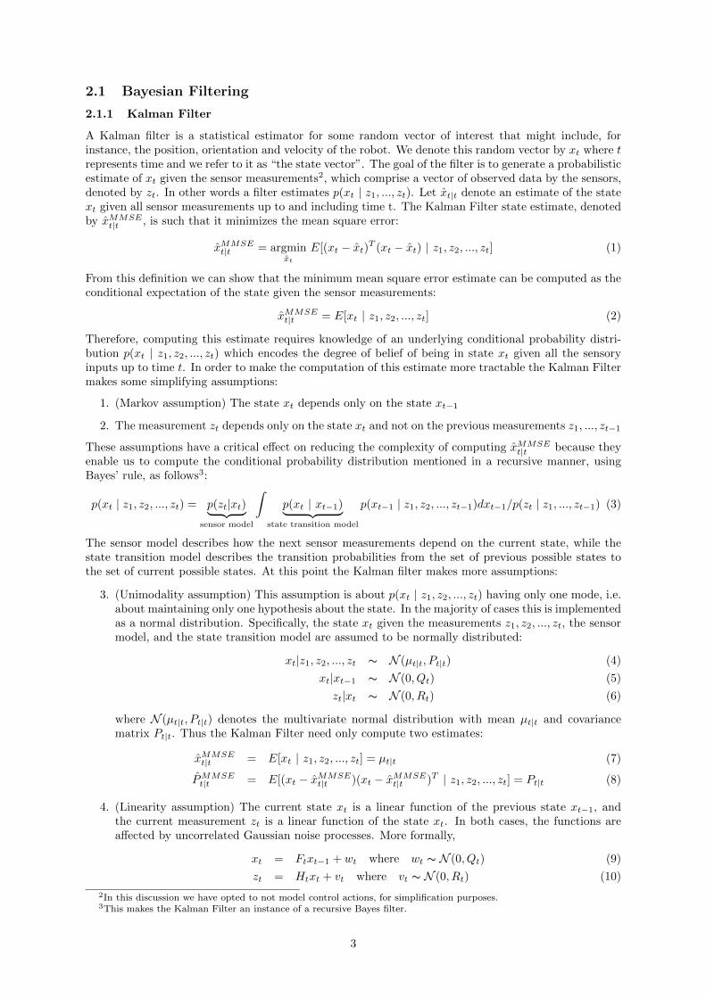
Algorithm 1: The main body of the RRT sampling algorithm. G=(V,E) denotes the tree representation,Sample is the function responsible for densely sampling the configuration space, and Extend is thefunction that generates a local path towards the new node, if possible.

idea among planning algorithms that fall in this category is that if they draw sufficiently many samplesfrom the free space, a solution path will be found with probability one, while if a path does not existthe algorithm might not terminate. These algorithms are called probabilistically-complete, and the restof this section is going to focus on providing a summary of recent developments in this area of pathplanning, in particular an analysis of the RRT, RRT*, and PRM sampling-based algorithms.

3.1 RRT

The Rapidly-exploring Random Tree (RRT) algorithm [5] randomly samples the free space trying toextend a tree from the initial configuration to the goal. A node represents a configuration that isreachable from the starting point, and an edge connects two configurations that are reachable via a smalllocal path that avoids obstacles. The algorithm, shown here as Alg. 1, terminates after a user-specifiednumber of times, or if the new sample is sufficiently close to the target configuration that a local pathcan connect them. If the latter is the case, we can trace a unique path from the start to the target.

One needs to be very careful and attentive when selecting the function Sample(i). This function,regardless of whether it is deterministic or random, must produce a sequence that is dense in the con-figuration space. Formally that means that the closure of the values of the sequence must completelycover the configuration space; informally, that means that for any possible configuration in the space thesequence can generate a value that is “close” to it.Sample(i) should also generate uniform samples that are not biased at particular regions. One of

the cases in which this problem arises is when one tries to uniformly sample from SO(3), the space of3D rotations. Rotation representation plays a major role here, because uniformly sampling three Eulerangles, for example, will not give rise to a uniform sampling of the space of rotations, due to the effect ofgimbal lock8. Uniform sampling methods that rely on the quaternion representation of rotations, whichdoes not suffer from such singularities, address this issue.

Another aspect with respect to which the choice of Sample(i) is important is the property of inter-ruptibility the planning algorithm. If for any reason we need to terminate the planning process earlierthan expected, we might want to have a uniformly dense covering of the space, as opposed to a finecovering of some regions but a very coarse covering of others. The metrics of dispersion and discrepancyhave been used in heuristics that regulate the covering of the sampling process, thereby reducing thedegree of randomness. Dispersion measures the radius of the largest uncovered ball in the configurationspace, and discrepancy measures the maximum difference between the number of points that were ex-pected to be sampled according to the uniform distribution and the number of points that were actuallysampled, in any subspace.

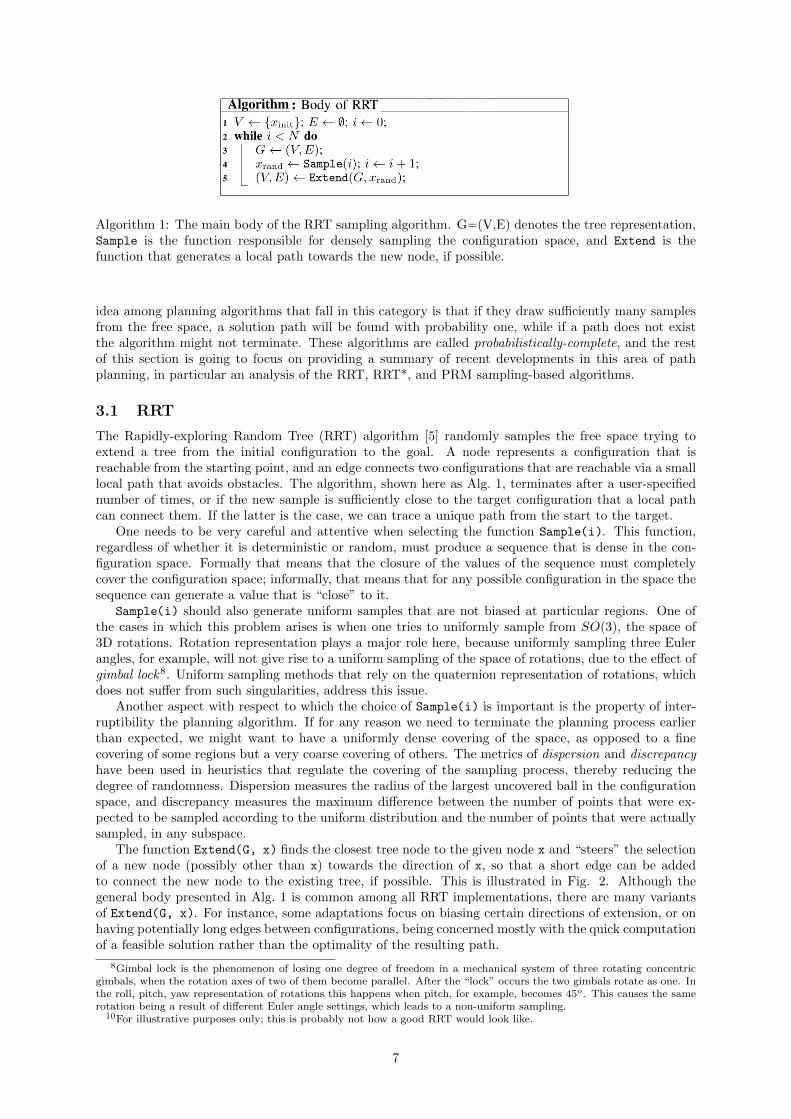
The function Extend(G, x) finds the closest tree node to the given node x and “steers” the selectionof a new node (possibly other than x) towards the direction of x, so that a short edge can be addedto connect the new node to the existing tree, if possible. This is illustrated in Fig. 2. Although thegeneral body presented in Alg. 1 is common among all RRT implementations, there are many variantsof Extend(G, x). For instance, some adaptations focus on biasing certain directions of extension, or onhaving potentially long edges between configurations, being concerned mostly with the quick computationof a feasible solution rather than the optimality of the resulting path.

8Gimbal lock is the phenomenon of losing one degree of freedom in a mechanical system of three rotating concentricgimbals, when the rotation axes of two of them become parallel. After the “lock” occurs the two gimbals rotate as one. Inthe roll, pitch, yaw representation of rotations this happens when pitch, for example, becomes 45o. This causes the samerotation being a result of different Euler angle settings, which leads to a non-uniform sampling.

10For illustrative purposes only; this is probably not how a good RRT would look like.

7

(a) (b)

(c) (d)

Figure 2: (a) Structure of the RRT at the previous iteration10. (b) Nearest neighbour tree node toSample(i) is computed. (c) Length of the new edge is limited to a user-specified threshold, η (d)Structure of the RRT at the end of the current iteration.

3.2 RRT*

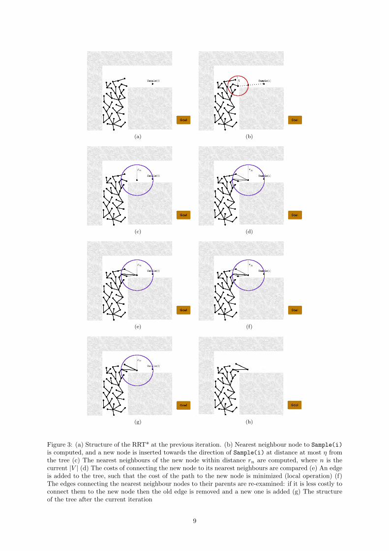
Approximately ten years after the initial publication of the RRT planner, and many reported practicalimplementations in real robot systems, the issue of whether the resulting path was optimal was still notsettled. The answer was recently shown to be negative in [6], provided the cost function satisfies somemild analytic requirements11. In particular it was proven that the probability that the RRT planneroutputs an optimal path tends to zero as the number of samples tends to infinity, even though theprobability that it will find a path tends to one. An alternative formulation, the RRT*, was proposedthat finds the optimal path with probability one as the number of samples tends to infinity. The RRT*planner consists of a modification of Extend(G, x) which is illustrated in Fig. 3. RRT* does notconnect the new node to its nearest neighbour; instead it searches all the nodes around a neighbourhoodof radius rn, trying to minimize the cost of reaching from the starting node to the new node, which is alocal operation. In addition, after the new node has been connected to the tree, all the existing parentsof its nearest neighbours are re-examined in order to see whether those nodes are reachable at a lowercost via the newly-inserted node. If so, the tree is rewired locally, and this local modification is whatenables the finding of an optimal path with high probability.

3.3 PRM

The RRT and RRT* algorithms that were mentioned above are aimed at single-query planning scenarios,meaning that if a new pair of starting and target configurations is input, then the old tree will have tobe discarded or heavily extended. The purpose of the Probabilistic Roadmap (PRM) sampling-basedplanning algorithm is to address multiple-query scenarios, without having to significantly modify thedata structure during the query stage. To this end, it requires a preprocessing step in which a graphrepresentation of the configuration space is constructed. Just like in the case of RRTs, the nodes aresampled configurations from the free space and edges are local paths that connect two configurationswithout leaving the free space. PRMs differ from RRTs in that a discrete graph search algorithm, such

11Lipschitz continuity, and therefore bounded derivative

8

(a) (b)

(c) (d)

(e) (f)

(g) (h)

Figure 3: (a) Structure of the RRT* at the previous iteration. (b) Nearest neighbour node to Sample(i)is computed, and a new node is inserted towards the direction of Sample(i) at distance at most η fromthe tree (c) The nearest neighbours of the new node within distance rn are computed, where n is thecurrent |V | (d) The costs of connecting the new node to its nearest neighbours are compared (e) An edgeis added to the tree, such that the cost of the path to the new node is minimized (local operation) (f)The edges connecting the nearest neighbour nodes to their parents are re-examined: if it is less costly toconnect them to the new node then the old edge is removed and a new one is added (g) The structureof the tree after the current iteration

9

Algorithm 4: The main body of the PRM sampling algorithm. Near(G, v, r) returns the set of nearestneighbour nodes of v, within a radius of r.

as Dijkstra’s, A* search, or Floyd-Warshall shortest paths, is required to find the best path between thestarting and ending configurations, whereas for RRTs the path is unique.

A simplified description of the PRM algorithm (s-PRM) is depicted in Alg. 4, which is essentiallyidentical to the construction of random geometric graphs. In fact, the radius of the neighbours of a givennode, r, is chosen in such a way that the graph will be connected with high probability, i.e. probabilitytending to one as the number of samples increases. It has been shown that this algorithm will find theoptimal path with high probability, if one exists, so it shares this property with the RRT*. One of theissues of practical interest is how many samples need to be drawn in order to guarantee that the s-PRMwill find a path if one exists, or in other words that the probability of error be sufficiently low. Thisissue was addressed in at least two works, [7, 8].

In [7] it was shown that the expected number of samples required are bounded above by a constantthat depends on the existence of positive-measure subspaces of the configuration space which can coverpart of paths from the target to the destination. This bound was based on an existence proof, and didnot provide a constructive method of actually computing the upper bound as a function of the tolerableerror, even though it showed that the probability of error decreases at an exponential rate in the numberof samples.

In [8] the probability of error of the s-PRM, as a function of the samples drawn, and the distanceof the path connecting the start and the goal from the obstacles, was actually computed. This is veryrelevant in a practical implementation because it allows the estimation of an upper bound on the numberof samples required to achieve the desired probability of error.

4 Clustering

Clustering algorithms deal with the question of how to group data points in such a way that “similar”points belong to the same group and there is no group containing “dissimilar” points. These algorithmsare useful in diverse branches of robotics from planning, to sensor data interpretation, to fault detec-tion. They enable the robot to reason and infer relations using the sparser representation of the grouprepresentatives rather than all data points. In addition to this functionality, clustering algorithms alsoenable robots to detect outliers in their incoming data streams. An outlier is any data point that eitherclearly does not belong to any cluster, or possibly one that has a high degree of ambiguity with respect tothe cluster it belongs to, while other points do not. There is a significant number of different clusteringtechniques, including among others:

• k-means, which, given a set of points in Rd, computes k centers in Rd, such that the total squareddistance of the given points to their closest clusters is minimized.

• maximum-likelihood estimate of the parameters of a mixture-of-Gaussians (or other distributions)that are going to represent the clusters, based on the given data points.

• spectral clustering, where the problem of finding k clusters of a given set of points in Rd is reducedto computing the eigenvalues and eigenvectors of a matrix that is created from the similarity scoresbetween each pair of points.

• hierarchical clustering, where the data is organized into trees, either bottom-up by grouping similarpoints, or top-down, by partitioning a set into more homogeneous components.

• any classification technique.

10

In this section we are going to focus on the properties of the first two techniques, namely k-meansand maximum-likelihood clustering via the Expectation-Maximization (EM) algorithm.

4.1 k-means

Given points x1, ..., xn ∈ Rd, the k-means problem is about finding k representatives c1, ..., ck ∈ Rd, suchthat the total squared distance of the given points to their closest cluster representatives is minimized,or more formally:

argminc1,...,ck

n∑i=1

minj=1,...,k

‖xi − cj‖2 (35)

One can show by algebraic arguments, as is done in [9], that if Cj is one of the clusters of points in theoptimal solution, then its representative, cj , must be the center of mass of Cj . So, if we let C1, ..., Ck bea partition of the points x1, ..., xn the problem can also be written as a combinatorial optimization:

argminC1,...,Ck

k∑j=1

∑x∈Cj

‖x− µ(Cj)‖2 (36)

where µ returns the mean of its input set of points.It was shown in [10] that the minimization of the cost function of Eq. (35) can be done in the

framework of gradient descent and Newton’s optimization method. For both cases, it was shown thatthere is a rigorous way of determining the descent rate, without resorting to heuristic tuning. This isimportant because it allows one to argue about the convergence of solutions to k-means in terms ofthe convergence rate of these different optimization methods. That said, even though the cost functiondecreases at each optimization step for each of these methods, convergence to local minima is almostsure [10].

4.2 Lloyd’s algorithm

The k-means problem has been shown to be NP-Hard, in fact even for the cases of k = 2 and planarpoints. The standard heuristic algorithm used in practice, known since the ’60s, is the following:

Step 1: Choose centers c1, ..., ck arbitrarilyStep 2: Set Cj = x : ‖x− cj‖ ≤ ‖x− ci‖ ∀i resolving cases of equidistant centers consistentlyStep 3: Set cj = µ(Cj). If the mean is undefined do not modify cj .Step 4: If no cluster Cj has changed since the last iteration stop, otherwise go to step 2.

In essence the algorithm produces an iterative refinement that converges to the Voronoi cells corre-sponding to the cluster centers, with each cell enclosing the points that are contained in that cluster. Thecomplexity of this heuristic algorithm has been the focus of many works, especially in the last five years.For instance, in [11] it was shown that the worst-case complexity of this algorithm is 2Ω(n), even whenthe input points lie on R2. Notwithstanding this result, Lloyd’s heuristic is perceived to be a relativelyefficient algorithm in practice, even though unfortunately, to the best of our knowledge, no average-caseanalysis has been performed to date.

Instead, what has been performed in recent years is a smoothed analysis of its running time [12].The main idea behind smoothed analysis is that given a worst-case input from an adversary, insteadof considering this pessimistic upper bound, we should consider the neighbourhood around said input.More specifically, if the worst-case input is perturbed by random Gaussian noise of standard deviationσ, then if we can show that the expected running time of the perturbed input is bounded above by apolynomial in (n, 1/σ) then this shows that the worst-case input is an “isolated” event. More formally,if In is an input of length n to an algorithm and T (In) is its running time then worst-case analysisconsiders max

InT (In), average-case analysis considers Ep(In) [T (In)], while smoothed analysis considers

maxIn

Eη∼N (η|0,σ2In×n) [T (In +η)]. In [12] it is shown that Lloyd’s heuristic has polynomial running time

using smoothed analysis.

11

4.3 k-means++

k-means++ is a modified version of Lloyd’s algorithm that is shown to be O(logk)-competitive on averagewith respect to the optimal clustering. The modification it proposes is on step 1, the selection of theinitial clusters:

Step 1.1: Let c1 be chosen uniformly at random from x1, ..., xnStep 1.2: Choose cj from x1, ..., xn with probability p(x) = min

c=c1,...,cj−1

‖x−c‖2/n∑i=1

minc=c1,...,cj−1

‖xi − c‖2

If we denote the cost in Eq. (36) by φ(X , C), where X = x1, ..., xn and C is a partition of X ,then [9] shows that the following will be true after the two cluster initialization steps mentioned above:Ep(C) [φ(X , C)] ≤ 8(lnk+ 2)φ(X , COPT ). Since the cost function decreases after each iteration of Lloyd’salgorithm, this competitive ratio holds until k-means++ terminates. In addition, [9] shows that this ratiois tight, by constructing an example of X where the expected cost is at least 2 lnk φ(X , COPT )

4.4 Maximum-likelihood clustering

While the k-means formulation mentioned above assigned each point xi to a unique cluster Cj , we canalso adopt the model whereby there is uncertainty in the cluster assignment for each data point [13, ch.9.2]. So, we make the assumption that the k clusters are represented as components in a mixture ofGaussians, which means that the data is assumed to be drawn from the density12:

pπ,c,Σ(x) =

k∑j=1

πj N (x|cj ,Σj) (37)

where π is a vector of probabilities with πj = p(zj = 1) being the probability of choosing cluster Cj .N (x|cj ,Σj) denotes the probability density of cluster Cj being centered at cj , the mean of the normal,and whose shape is determined by the covariance matrix Σj . In contrast to this formulation, k-meansrepresents clusters only by their centers. Considering all this, maximizing the likelihood of the givendata points means:

argmaxπ,c,Σ

pπ,c,Σ(X ) = argmaxπ,c,Σ

n∏i=1

pπ,c,Σ(xi) = argmaxπ,c,Σ

n∑i=1

ln(pπ,c,Σ(xi)) (38)

At a local maximum of Eq. (38) the partial derivatives with respect to cj , Σj , and πj are all zero, fromwhich we get:

cj =

n∑i=1

wijxi/

n∑i=1

wij (39)

Σj =

n∑i=1

wij(xi − cj)(xi − cj)T /n∑i=1

wij (40)

πj =

n∑i=1

wij/n (41)

where (42)

wij = πj N (xi|cj ,Σj)/k∑r=1

πrN (xi|cr,Σr) = p(zj = 1|xi) (43)

The probabilities wij can be regarded as the degree to which point xi belongs to cluster Cj . One wayto perform the maximization and avoid the interdependency between the different parameters is EM(Expectation-Maximization) [13, ch. 9.4], which is a two-phase iterative optimization method:

Step 1: Initialize π, c,Σ and evaluate the log-likelihood in Eq. (38)Step 2: Evaluate wij , keeping πj , cj ,Σj fixed.Step 3: Evaluate πj , cj ,Σj , keeping wij fixed.

12π ∈ Rk, c ∈ Rd×k,Σ ∈ Rd×(d+k) are regarded as model parameters for the k clusters.

12

Step 4: Stop if the new log-likelihood or the parameters have converged, otherwise go to step 2.

The EM iterations guarantee that the value of the log-likelihood will be non-decreasing and it will reach astationary point. In general, however, it is not always guaranteed that a local maximum will be reached,and examples of data points and the distributions that generated them have been presented, in which theEM iterations converge to a saddle point. These pathological situations do not arise in the case wherethe data are sampled from a mixture of Gaussians.

5 Classification and ensemble methods

Classification is the problem of correctly assigning a label y ∈ 1, ...,m to an input x ∈ Rd, which hasnot been seen before, based on a known set of training examples Dn = (xi, yi), i = 1...n, which havebeen drawn from an unknown distribution. If the possible range of the labels is y ∈ R then we speak ofregression instead of classification. Our goal is to construct a classifier gDn(x) that estimates the truedistribution p(y|x) by trying to minimize a loss function. An example of a loss function in the case ofm-class classification is Ep(x,y|Dn)

[1[gDn (x)6=y]|Dn

]= p(gDn(x) 6= y|Dn), while in the case of regression

we might use the mean squared error Ep(x,y|Dn)

[(gDn(x)− y)2|Dn

]. These two loss functions, although

frequently used, might not be the most appropriate for a given problem, so one must be attentive whenchoosing them. Although numerous classifiers have been proposed in the literature, such as:

• k-nearest neighbours

• decision trees

• support vector machines (SVMs)

• naive Bayes

• neural networks

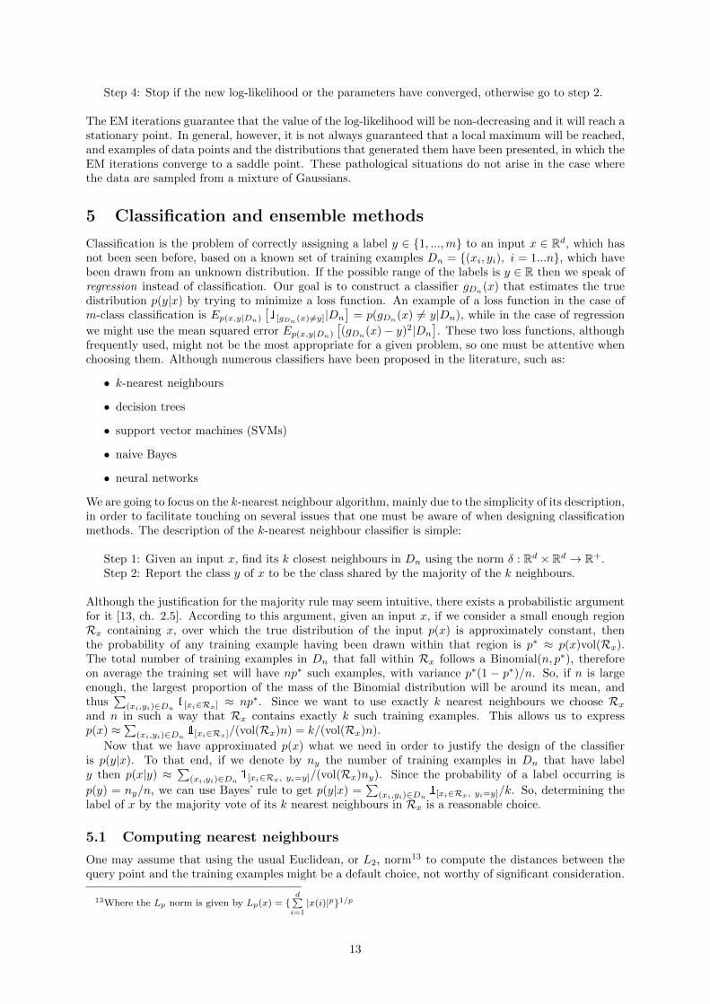
We are going to focus on the k-nearest neighbour algorithm, mainly due to the simplicity of its description,in order to facilitate touching on several issues that one must be aware of when designing classificationmethods. The description of the k-nearest neighbour classifier is simple:

Step 1: Given an input x, find its k closest neighbours in Dn using the norm δ : Rd × Rd → R+.Step 2: Report the class y of x to be the class shared by the majority of the k neighbours.

Although the justification for the majority rule may seem intuitive, there exists a probabilistic argumentfor it [13, ch. 2.5]. According to this argument, given an input x, if we consider a small enough regionRx containing x, over which the true distribution of the input p(x) is approximately constant, thenthe probability of any training example having been drawn within that region is p∗ ≈ p(x)vol(Rx).The total number of training examples in Dn that fall within Rx follows a Binomial(n, p∗), thereforeon average the training set will have np∗ such examples, with variance p∗(1 − p∗)/n. So, if n is largeenough, the largest proportion of the mass of the Binomial distribution will be around its mean, andthus

∑(xi,yi)∈Dn 1[xi∈Rx] ≈ np∗. Since we want to use exactly k nearest neighbours we choose Rx

and n in such a way that Rx contains exactly k such training examples. This allows us to expressp(x) ≈

∑(xi,yi)∈Dn 1[xi∈Rx]/(vol(Rx)n) = k/(vol(Rx)n).

Now that we have approximated p(x) what we need in order to justify the design of the classifieris p(y|x). To that end, if we denote by ny the number of training examples in Dn that have labely then p(x|y) ≈

∑(xi,yi)∈Dn 1[xi∈Rx, yi=y]/(vol(Rx)ny). Since the probability of a label occurring is

p(y) = ny/n, we can use Bayes’ rule to get p(y|x) =∑

(xi,yi)∈Dn 1[xi∈Rx, yi=y]/k. So, determining thelabel of x by the majority vote of its k nearest neighbours in Rx is a reasonable choice.

5.1 Computing nearest neighbours

One may assume that using the usual Euclidean, or L2, norm13 to compute the distances between thequery point and the training examples might be a default choice, not worthy of significant consideration.

13Where the Lp norm is given by Lp(x) = d∑

i=1|x(i)|p1/p

13

Figure 5: On the x-axis is the dimensionality d. On the y-axis DMAXpd −DMINp

d is shown from datagenerated uniformly at random. The norms used: (a) the L3 (b) the L2 (c) the L1 (d) the L2/3 (e) theL2/5.

In [14, 15] the authors point out that this is often a mistaken assumption when the dimensionality of thedata is high. They show that using Lp norms where p > 1 might lead to a phenomenon where there isnot much difference between the farthest and the closest points as the dimensionality of the data goes toinfinity, which implies that any algorithm based on nearest neighbour search might not be meaningful,and might suffer from a high ratio of false positives. In robotics nearest neighbor search is ubiquitous,as many of the representations of the sensor data use high-dimensional vectors14.

Specifically, given an input query point x ∈ Rd let the Lp distance of the farthest neighbour of xin the training set Dn be DMAXp

d , and similarly for that of the closest training example, let it beDMINp

d . Let us consider x to be the origin of the coordinate system, without loss of generality, so thatDMAXp

d = max‖x‖p | (x, y) ∈ Dn, x ∈ Rd. Then [15] proves the following theorem:

Theorem 1. If limd→∞ var(‖x‖p

E[‖x‖p] ) = 0 then ∀ε > 0 limd→∞ p(DMAXpdDMINpd

≤ 1 + ε) = 1

Under the given precondition, DMAXpd converges in probability to DMINp

d . Settings in which theprecondition holds and others, where it does not, are identified in the paper. In particular, it mentionsthat in scenarios where the query point belongs to a clearly defined cluster in the training set theprecondition is not generally satisfied, whereas in the case where the training examples and the querypoints are drawn as i.i.d. samples then it does.Based on the theorem above, the work in [14] examines the values of p for which the corresponding Lpnorm leads to a high difference between DMAXp

d and DMINpd as d → ∞. The main theorem that

illustrates their results is:

Theorem 2. If a point has n − 1 neighbours following an arbitrary distribution then there exists a

constant Cp > 0 such that Cp ≤ limd→∞E[DMAXpd−DMINpd ]

d1/p−1/2 ≤ (n− 1)Cp

This means that E[DMAXpd − DMINp

d ] grows as d1/p−1/2 while d → ∞. So, for p > 2 it tendsto 0 while for p < 2 it tends to infinity, which, according to the authors, will help differentiate nearestneighbours in high dimensions. Therefore, they recommend using the L1 norm, or even a fractional Lpnorm with p < 1, in favour of the other Lp norms, including the Euclidean, as shown by their results onFig. 5.

14For instance, feature extraction methods from images are often associated with a high-dimensional image descriptorthat describes the local structure of the image’s intensity gradient. This is also the case in motion planning algorithms aswe mentioned in section 3.

14

5.2 Bagging classifiers

Many researchers have studied the question of whether combining different classifiers into a single outputcontributes significantly, if at all, to a lower misclassification rate. One of the resulting methods isbootstrap aggregation, or “bagging” [16], according to which several classifiers are combined by averagingin the case of real-valued labels, or by majority rule in the case of finite labels. Ideally, this method

requires many training sets D(j)n , j = 1, ..., s, all independently sampled from a distribution D, and all

of whose examples are i.i.d., but realistically, one usually has access to only one training set Dn. Inthat case we can randomly choose with replacement from Dn to form the training sets. Hence, given sreal-valued classifiers g

D(j)n

(x) the bagging method outputs g(x) = ED[gD

(j)n

(x)]. For a fixed pair (x, y)

the error of a single real-valued classifier is:

ED[(gD(j)(x)− y)2] = y2 − 2yED[gD(j)(x)] + ED[gD(j)(x)2] (44)

≥ y2 − 2yg(x)ED[gD(j)(x)]2 (45)

= (y − g(x))2 (46)

so the expected error over all pairs (x, y) is not increased if we use the aggregate classifier g(x). Thequestion of when does bagging significantly decrease the expected error depends on how big the differenceED[gD(j)(x)2]−ED[gD(j)(x)]2 ≥ 0 is. Equivalently, this means that the higher the variance varD[gD(j)(x)]of each classifier’s performance on different training sets, the larger the improvement of the baggedclassifier will be.

Similar results are shown in [16] for classifiers whose range is a finite set of labels: if the componentclassifiers gD(j)(x) can predict the modes of the true distribution p(y|x) frequently, but not necessarilywith frequency p(y|x), then the bagged classifier g(x) will show a significant improvement over thecomponent classifiers. The higher this order-correctness property of the component classifiers, the betterthe resulting g(x) will be. If, on the other hand, this property is not satisfied very often then the resultingclassifier may end up performing worse than its components, unlike in the case of real-valued classifiers.

5.3 Boosting classifiers

Another way of combining individual classifiers into an aggregate, improved one, is boosting [17]. Themain idea behind it is that multiple “weak” classifiers can be combined into an accurate classifier bycarefully weighting the individual components. By “accurate” it is meant that the classification error ofthe final classifier on the training examples can become arbitrarily small given sufficient examples andweak predictors. The most well-known boosting algorithm is Adaptive Boosting, or AdaBoost, which isa supervised learning method, so the weak classifiers need to be trained on labeled examples. At eachtraining iteration t = 1, ..., T , AdaBoost trains a new weak classifier gt(x) : Rd → −1,+1 which isdesigned in such a way that it performs better than random classification, based on the training dataDn, where it is assumed in this case that the labels are binary. For the next iteration AdaBoost assigns

more weight w(t+1)i to the training examples that gt(x) misclassified, and after all iterations are done

the resulting classifier g(x), a linear combination of the weak classifiers, is returned. The steps of thealgorithm are outlined below:

Step 1: assign uniform weights w(1)i = 1/n to all training examples for all i = 1, ..., n

Step 2: repeat steps 3 to 6 from t = 1, ..., T

Step 3: find a gt : Rd → −1,+1 that minimizes the weighted error∑ni=1 w

(t)i 1[gt(xi)6=yi]

Step 4: evaluate the error percentage of the classifier, εt =∑ni=1 w

(t)i 1[gt(xi)6=yi]/

∑ni=1 w

(t)i

Step 5: weight to be assigned to gt in the final classifier is αt = ln( 1−εtεt

)

Step 6: update the weights to focus on misclassified examples, w(t+1)i = w

(t)i exp(αt1[gt(xi) 6=yi])

Step 7: output g(x) = sign(∑Tt=1 αtgt(x))

The choice of weights αt for each component and the weight update equations w(t)i are not arbitrary, of

15

course. [17] shows that the training error of AdaBoost satisfies:

n∑i=1

1[g(xi)6=yi] ≤n∑i=1

exp(−yiT∑t=1

αtgt(xi)) = n

T∏t=1

Zt ≤ nexp(−2

T∑t=1

(1/2− εt)2) (47)

where

Zt =

n∑i=1

w(t)i exp(−αtyigt(xi)) (48)

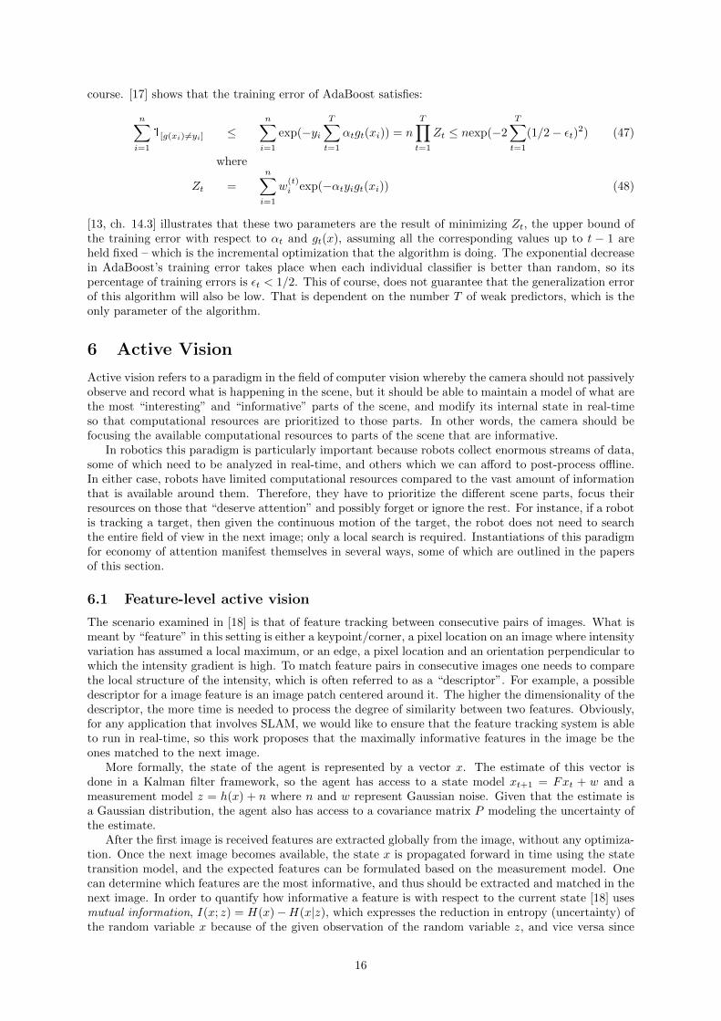
[13, ch. 14.3] illustrates that these two parameters are the result of minimizing Zt, the upper bound ofthe training error with respect to αt and gt(x), assuming all the corresponding values up to t − 1 areheld fixed – which is the incremental optimization that the algorithm is doing. The exponential decreasein AdaBoost’s training error takes place when each individual classifier is better than random, so itspercentage of training errors is εt < 1/2. This of course, does not guarantee that the generalization errorof this algorithm will also be low. That is dependent on the number T of weak predictors, which is theonly parameter of the algorithm.

6 Active Vision

Active vision refers to a paradigm in the field of computer vision whereby the camera should not passivelyobserve and record what is happening in the scene, but it should be able to maintain a model of what arethe most “interesting” and “informative” parts of the scene, and modify its internal state in real-timeso that computational resources are prioritized to those parts. In other words, the camera should befocusing the available computational resources to parts of the scene that are informative.

In robotics this paradigm is particularly important because robots collect enormous streams of data,some of which need to be analyzed in real-time, and others which we can afford to post-process offline.In either case, robots have limited computational resources compared to the vast amount of informationthat is available around them. Therefore, they have to prioritize the different scene parts, focus theirresources on those that “deserve attention” and possibly forget or ignore the rest. For instance, if a robotis tracking a target, then given the continuous motion of the target, the robot does not need to searchthe entire field of view in the next image; only a local search is required. Instantiations of this paradigmfor economy of attention manifest themselves in several ways, some of which are outlined in the papersof this section.

6.1 Feature-level active vision

The scenario examined in [18] is that of feature tracking between consecutive pairs of images. What ismeant by “feature” in this setting is either a keypoint/corner, a pixel location on an image where intensityvariation has assumed a local maximum, or an edge, a pixel location and an orientation perpendicular towhich the intensity gradient is high. To match feature pairs in consecutive images one needs to comparethe local structure of the intensity, which is often referred to as a “descriptor”. For example, a possibledescriptor for a image feature is an image patch centered around it. The higher the dimensionality of thedescriptor, the more time is needed to process the degree of similarity between two features. Obviously,for any application that involves SLAM, we would like to ensure that the feature tracking system is ableto run in real-time, so this work proposes that the maximally informative features in the image be theones matched to the next image.

More formally, the state of the agent is represented by a vector x. The estimate of this vector isdone in a Kalman filter framework, so the agent has access to a state model xt+1 = Fxt + w and ameasurement model z = h(x) + n where n and w represent Gaussian noise. Given that the estimate isa Gaussian distribution, the agent also has access to a covariance matrix P modeling the uncertainty ofthe estimate.

After the first image is received features are extracted globally from the image, without any optimiza-tion. Once the next image becomes available, the state x is propagated forward in time using the statetransition model, and the expected features can be formulated based on the measurement model. Onecan determine which features are the most informative, and thus should be extracted and matched in thenext image. In order to quantify how informative a feature is with respect to the current state [18] usesmutual information, I(x; z) = H(x)−H(x|z), which expresses the reduction in entropy (uncertainty) ofthe random variable x because of the given observation of the random variable z, and vice versa since

16

Figure 6: An example of a saliency map constructed from a color, an intensity, and an orientationcontrast layer.

it is symmetric. In addition, one can also compute I(zi; zj) which describes to what degree two featuresare independent, which if it is low then it might possibly be redundant to attempt to measure both.

6.2 Image-level active vision

Aside from quantifying which features are going to be the most informative, we may ask: given an imagethat we have not seen before, what are the parts of it that are the most informative for the purposeof searching for a specific object? This is the scenario examined in [19], the main idea behind whichis to perform gaze planning on a coarse, but fast-to-compute, visual saliency map and then apply acomputationally expensive accurate detector for the object of interest at the parts that were deemed tobe more salient.

The construction of the saliency map which is a critical component of this paper was described in [20].This map is essentially a linear combination of different processed versions (layers) of the original image,as shown in Fig. 6. Some of these layers measure intensity contrast, others measure local color differencesbetween the three color channels, and the third group measures local contrasts in orientation. Takeninto isolation, each of these three groups of layers has desirable properties for low-level keypoint features.After the saliency map has been computed, [19] detects the most salient locations on the map and definesa gaze πi in pixel coordinates for each of those locations. Assuming that the total number of gazes isgoing to be small, the proposed method considers all the possible gaze sequences, in other words, searchplans π, for the object of interest.

This work assumes the existence of a detector model p(yt|xt) which is the probability that the objectdetector will detect the object or not, yt ∈ 0, 1, at the image location xt. This density is estimatedoffline from training data and it depends on the particular type of object that is being searched for,but not on the gaze plan. For example, computer monitors were objects of interest in the experimentalsection of this work, and in the training set which was used monitors usually appeared on the bottompart of the image, not on the ceiling, so this will be encoded in the detector model.

For each fixed gaze sequence π of length T , there is a cost Cπ associated with it. The cost functionproposed in [19] is

Cπ =

T∑t=1

λt Ep(x0:T ,y1:T | π) [H(p(xt | y1:t, π)−H(p(xt−1 | y1:t−1, π)))] (49)

where the difference in entropy measures the increase in uncertainty about the object’s location aroundgaze πt compared to that around gaze πt−1, given the history of detector responses. λ is a discountfactor for this increase, and the planning horizon is up to T , the length of the gaze sequence. The gazesequence with the smallest cost is the one chosen for actual applications of the object detector.

This method was shown to perform better than the sequence obtained by ordering the gazes in thesaliency map based on their importance. One of the conclusions of this work’s experiments was that it hasless false positives than applying the object detector throughout the entire image, which is an additionalreason to motivate this kind of active vision approaches, aside from the reduced computational load.

17

6.3 Viewpoint-level active vision

In [21] the problem of object recognition is examined in the context of active vision. Here an agentequipped with a camera operates in a 3D world and wants to estimate the identity y ∈ 1, ..., k andthe orientation of an object with respect to a global frame of reference. One of the difficulties associatedwith this problem is that if an object is viewed from a specific viewpoint there might be many plausiblehypotheses about its class. To resolve this ambiguity one therefore might have to consider more thanone viewpoint. Efficiently selecting the least number of informative viewpoints required to recognize anobject is the main problem addressed in [21]. This work makes some simplifying assumptions:

First, the agent’s position is assumed to be constrained on the surface of a viewing sphere whosecenter is one of the objects of interest. In other words, the agent is not allowed to approach the objector zoom in, but only to pan and tilt, so its position is actually a viewpoint v = (φ1, φ2) on the viewingsphere15. Second, the orientation of the object that is being viewed is discretized, and is assumed tobe indexed by θ ∈ 1, ..., Nθ which identifies a finite number of possible 3D orientation values. Third,the scene is assumed to have only one light source, whose 3D position is also discretized and assumedto be indexed by l ∈ 1, ..., Nl, which identifies a finite number of possible positions. Fourth, the sceneincludes only one of the k objects.

The measurement model of the camera z = h(y, v, θ, l) is assumed to be estimated offline using aspecific camera and lighting model, and due to its uncertainty it is also regarded as a conditional densityp(z|y, v, θ, l) whose parameters are known. The main idea in [21] is to choose the next viewpoint vt+1

so that it resolves the most significant ambiguity, i.e. a viewpoint from which there are at least twovery different, yet plausible, hypotheses about y, θ given the past measurements and viewpoints. Tohave a plausible hypothesis according to this criterion, means that the following probability should bemaximized:

p(y, θ|Mt) =

Nl∑l=1

p(y, θ, l|Mt) ∝Nl∑l=1

p(zt|y, θ, l, vt)p(y, θ, l|Mt−1) (50)

where Mt = zt, vt, ..., z1, v1 is the set of past measurements and viewpoints. [21] interprets having twodifferent hypotheses as maximizing the following divergence for two hypotheses (y, θ) and (y′, θ′):

J(p(zt+1 | y, θ, vt+1,Mt) || p(zt+1 | y′, θ′, vt+1,Mt)) (51)

where J(p||q) = DKL(p||q) + DKL(q||p) is the so called Jeffrey’s divergence, and DKL is the Kullback-Leibler divergence. To make the computation that is necessary in Jeffrey’s divergence16 a bit clearer, weobserve that after applying Bayes’ rule and some independence assumptions:

p(zt+1 | y, θ, vt+1,Mt) =

Nl∑l=1

p(zt+1 | y, θ, l, vt+1) p(y, θ, l | Mt) / p(y, θ | Mt) (52)

which means that what needs to be modelled is only the measurement model p(z|y, θ, l, v) and theinitial value p(y, θ, l|M1) because the rest can be computed recursively via dynamic programming. So,in summary the proposed criterion for viewpoint selection is the following:

v∗t+1 = argmaxvt+1

k∑y=1

Nθ∑θ=1

k∑y′=1

Nθ∑θ′=1

p(y, θ|Mt)p(y′, θ′|Mt)J(p(zt+1 | y, θ, vt+1,Mt) || p(zt+1 | y′, θ′, vt+1,Mt)) (53)

This criterion is compared in [21] against the mutual information criterion of choosing the next viewpointthat maximizes the mutual information between (y, θ) and zt+1|vt+1. The comparison is performed onsynthetic scenes, where it is shown experimentally that (53) does as well as the mutual informationcriterion, which is reported to take “several days”17 to recognize all the objects in the database, butabout 1000 times faster.

15The agent is keeping the object in the center of its field of view16It is mentioned in the paper that if p and q are Gaussian distributions then J(p||q) has a closed form.17Of course, without looking at the source code, and without knowing which efforts were made to optimize the compu-

tation, this claim is very hard to verify.

18

References

[1] M. J. Stanway, “Contributions to Automated Realtime Underwater Navigation,” Ph.D. Thesis,M.I.T. and Woods Hole Oceanographic Institution, 2012.

[2] A. J. Davison, I. D. Reid, N. D. Molton, and O. Stasse, “MonoSLAM: real-time single cameraSLAM.” IEEE transactions on pattern analysis and machine intelligence, vol. 29, no. 6, pp. 1052–1067, Jun. 2007.

[3] S. J. Julier and J. K. Uhlmann, “A New Extension of the Kalman Filter to Nonlinear Systems,” inThe 11th International Symposium on Aerospace/Defence Sensing, Simulation and Controls, 1997.

[4] F. Dellaert and M. Kaess, “Square Root SAM: Simultaneous Localization and Mapping via SquareRoot Smoothing,” International Journal of Robotics Research, vol. 25, no. 12, pp. 1181–1203, 2006.

[5] S. M. Lavalle, Planning Algorithms, Chapter 5: Sampling-based Motion Planning. CambridgeUniversity Press, 2006.

[6] S. Karaman and E. Frazzoli, “Incremental Sampling-based Algorithms for Optimal Motion Plan-ning,” in Robotics: Science and Systems (RSS), Zaragoza, Spain, 2010.

[7] A. Ladd, “Generalizing the analysis of PRM,” in IEEE International Conference on Robotics andAutomation (ICRA), 2002, pp. 2120–2125.

[8] L. Kavraki, M. Kolountzakis, and J.-C. Latombe, “Analysis of Probabilistic Roadmaps for pathplanning,” IEEE Transactions on Robotics and Automation, vol. 14, no. 1, pp. 166–171, 1998.

[9] D. Arthur and S. Vassilvitskii, “k-means++ : The Advantages of Careful Seeding,” in Symposiumon Discrete Algorithms (SODA), vol. 8, 2007, pp. 1027–1035.

[10] L. Bottou, “Convergence Properties of the K-Means Algorithms,” in Advances in Neural InformationProcessing Systems (NIPS), 1995, pp. 585–592.

[11] A. Vattani, “k-means Requires Exponentially Many Iterations Even in the Plane,” Discrete &Computational Geometry, vol. 45, no. 4, pp. 596–616, Mar. 2011.

[12] D. Arthur, B. Manthey, and H. Roglin, “Smoothed Analysis of the k-Means Method,” Journal ofthe ACM, vol. 58, no. 5, pp. 1–31, Oct. 2011.

[13] C. Bishop, Pattern Recognition and Machine Learning, 1st ed. Springer, 2006.

[14] C. Aggarwal, A. Hinneburg, and D. Keim, “On the Surprising Behavior of Distance Metrics in HighDimensional Space,” in International Conference on Database Theory, 1999, pp. 420–434.

[15] K. Beyer, J. Goldstein, R. Ramakrishnan, and U. Shaft, “When Is Nearest Neighbor Meaningful ?”in International Conference on Database Theory, 1999, pp. 217–235.

[16] L. Breiman, “Bagging Predictors,” Journal of Machine Learning, vol. 24, no. 2, pp. 123–140, 1996.

[17] R. Schapire, “The Boosting Approach to Machine Learning: An Overview,” MSRI Workshop onNonlinear Estimation and Classification, 2003.

[18] A. J. Davison, “Active Search for Real-Time Vision,” in IEEE International Conference on Com-puter Vision, 2005, pp. 66–73.

[19] J. Vogel and N. D. Freitas, “Target-directed attention : Sequential decision-making for gaze plan-ning,” in IEEE International Conference on Robotics and Automation, 2008, pp. 2372–2379.

[20] L. Itti, C. Koch, and E. Niebur, “A model of saliency-based visual attention for rapid scene analysis,”IEEE Transactions on Pattern Analysis and Machine Intelligence, vol. 20, no. 11, pp. 1254–1259,1998.

[21] C. Laporte and T. Arbel, “Efficient Discriminant Viewpoint Selection for Active Bayesian Recogni-tion,” International Journal of Computer Vision, vol. 68, no. 3, pp. 267–287, May 2006.

19