THEORETICAL REVIEW

The drift diffusion model as the choice rule in reinforcementlearning

Mads Lund Pedersen1,2& Michael J. Frank3

& Guido Biele1,4

Published online: 13 December 2016# Psychonomic Society, Inc. 2016

Abstract Current reinforcement-learning models often as-sume simplified decision processes that do not fully reflectthe dynamic complexities of choice processes. Conversely,sequential-sampling models of decision making account forboth choice accuracy and response time, but assume that de-cisions are based on static decision values. To combine thesetwo computational models of decision making and learning,we implemented reinforcement-learning models in which thedrift diffusion model describes the choice process, therebycapturing both within- and across-trial dynamics. To exempli-fy the utility of this approach, we quantitatively fit data from acommon reinforcement-learning paradigm using hierarchicalBayesian parameter estimation, and compared model variantsto determine whether they could capture the effects of stimu-lant medication in adult patients with attention-deficit hyper-activity disorder (ADHD). The model with the best relative fitprovided a good description of the learning process, choices,and response times. A parameter recovery experiment showed

that the hierarchical Bayesian modeling approach enabled ac-curate estimation of the model parameters. The model ap-proach described here, using simultaneous estimation ofreinforcement-learning and drift diffusion model parameters,shows promise for revealing new insights into the cognitiveand neural mechanisms of learning and decision making, aswell as the alteration of such processes in clinical groups.

Keywords Decisionmaking . Reinforcement learning .

Bayesianmodeling .Mathematical models

Computational models have greatly contributed to bridging thegap between behavioral and neuronal accounts of adaptivefunctions such as instrumental learning and decision making(Forstmann & Wagenmakers, 2015). The discovery that learn-ing is driven by phasic bursts of dopamine coding a rewardprediction error can be traced to reinforcement-learning (RL)models (Glimcher, 2011; Montague, Dayan, & Sejnowski,1996; Rescorla & Wagner, 1972). Similarly, the current under-standing of the neural mechanisms of simple decision makingclosely resembles the processes modeled in sequential-sampling models of decision making (Smith & Ratcliff, 2004).

RLmodels have been extended to account for the complex-ities of learning—for example, by proposing different valua-tions (Ahn, Busemeyer, Wagenmakers, & Stout, 2008;Busemeyer & Stout, 2002) and updating of gains and losses(Frank, Moustafa, Haughey, Curran, & Hutchison, 2007;Gershman, 2015), by accounting for the role of working mem-ory during learning (Collins & Frank, 2012), and by introduc-ing adaptive learning rates (Krugel, Biele, Mohr, Li, &Heekeren, 2009). In contrast, the choice process during instru-mental learning in RL is typically modeled with simple choicerules such as the softmax logistic function (Luce, 1959),which do not capture the dynamics of decision making (and

Electronic supplementary material The online version of this article(doi:10.3758/s13423-016-1199-y) contains supplementary material,which is available to authorized users.

* Mads Lund Pedersenm.l.pedersen@psykologi.uio.no

* Guido Bieleguido.biele@neuro-cognition.org

1 Department of Psychology, University of Oslo, Oslo, Norway2 Intervention Centre, Oslo University Hospital, Rikshospitalet,

Oslo, Norway3 Department of Cognitive, Linguistic & Psychological Sciences,

Brown Institute for Brain Science, Brown University,Providence, Rhode Island, USA

4 Norwegian Institute of Public Health, Oslo, Norway

Psychon Bull Rev (2017) 24:1234–1251DOI 10.3758/s13423-016-1199-y

hence are unable to account for choice latencies). Conversely,these complexities are described well by the class ofsequential-sampling models of decision making, which in-cludes the drift diffusion model (DDM; Ratcliff, 1978), thelinear ballistic accumulator model (Brown & Heathcote,2008), the leaky competing accumulator model (Usher &McClelland, 2001), and decision field theory (Busemeyer &Townsend, 1993). The DDM of decision making is a widelyused sequential-sampling model (Forstmann, Ratcliff, &Wagenmakers, 2016; Ratcliff & McKoon, 2008; Wabersich& Vandekerckhove, 2013; Wiecki, Sofer, & Frank, 2013),which assumes that choices are made by continuouslysampling noisy decision evidence accumulating until adecision boundary is reached in favor of one of two alter-natives. The key advantage of sequential-sampling modelslike the DDM is that they extract more information fromchoice data by simultaneously fitting response time (RT;and the distributions thereof) and accuracy (or choicedirection) data. Combining the dynamic learning process-es across trials modeled by RL with the fine-grainedaccount of decision processes within trials afforded bysequential-sampling models could therefore provide aricher description and new insights into decision process-es in instrumental learning.

To draw on the advantages of both RL and sequential-sampling models, the goal of this article is to construct acombined model that can improve understanding of thejoint latent learning and decision processes in instrumen-tal learning. A similar approach has been described byFrank et al. (2015), who modeled instrumental learningby combining Bayesian updating as a learning mechanismwith the DDM as a choice mechanism. The innovation ofthe research described here is that we combined a detaileddescription of both RL and choice processes, allowing forsimultaneous estimation of their parameters. The benefitof using the DDM as the choice rule in an RL model isthat a combined model can capture various factors, in-cluding the sensitivity to expected rewards, how they areupdated by prediction errors, and the trade-off betweenspeed versus accuracy during response selection. This en-deavor can help decompose mechanisms of choice andlearning in a richer way than could be accomplished byeither RL or DDM models alone, while also laying thegroundwork to further investigate the neural underpin-nings of these subprocesses by fitting model parametersbased on neural regressors (Cavanagh, Wiecki, & Cohen,2011; Frank et al., 2015).

One hurdle for the implementation of complex modelsof learning and decision making has traditionally been thedifficulty to fit models with a large number of parameters.The advancement of methods for Bayesian parameter es-timation in hierarchical models has helped address thisproblem (Lee & Wagenmakers, 2014; Wiecki et al.,

2013). A hierarchical Bayesian approach improves theestimation of individual parameters by assuming that theparameters for individuals are drawn from group distribu-tions (Kruschke, 2010), yielding mutually constrained es-timates of group and individual parameters that can im-prove parameter recovery for individual subjects (Gelmanet al., 2013).

In the following sections, we will describe RL modelsand the DDM in detail, before explaining and justifying acombined model. We will propose potential mechanismsinvolved in instrumental learning, and describe modelsexpressing these mechanisms. Next, we compare how wellthese models describe data from an instrumental-learningtask in humans. To show that combining RL and theDDM is able to account for data and provide new insight,we will demonstrate that the best-fitting model can disen-tangle effects of stimulant medication on learning and de-cision processes in attention-deficit hyperactivity disorder(ADHD). Finally, to ensure that the model parameterscapture the submechanisms they are intended to describe,we show that the generated parameters can successfully berecovered from simulated data.

Reinforcement-learning models

RL models were developed to describe associative andinstrumental learning (Bush & Mosteller, 1951; Rescorla& Wagner, 1972). The central tenet to these models isthat learning is driven by unexpected outcomes—forexample, the surprising occurrence or omission ofreward, in associative learning, or when an action results ina larger or smaller reward than is expected, in instrumentallearning. An unexpected event is captured by the predictionerror (PE) signal, which describes the difference between theobserved and predicted rewards. The PE signal thus generatesan updated reward expectation by correcting pastexpectations.

The strong interest in RL in cognitive neuroscience wasamplified by the finding that the reward PE is signaled bymidbrain dopaminergic neurons (Montague et al., 1996;Schultz, Dayan, & Montague, 1997), which can then alterexpectations and subsequent choices by modifying synapticplasticity in the striatum (see Collins & Frank, 2014, for areview and models).

RL models typically consist of, at least, an updatingmechanism for adapting reward expectations of choice op-tions, and an action selection policy that describes howchoices between options are made. A popular learning al-gorithm is the delta learning rule (Bush & Mosteller, 1951;Rescorla & Wagner, 1972), which can be used to describetrial-by-trial instrumental learning. According to this algo-rithm, the reward value expectation for the chosen option i

Psychon Bull Rev (2017) 24:1234–1251 1235

on trial t, Vi(t), is calculated by summing the reward ex-pectation from the previous trial and the reward PE:

Vi tð Þ ¼ Vi t−1ð Þ þ η Rewardi t−1ð Þ−Vi t−1ð Þ½ �: ð1Þ

The PE is weighted with a learning rate parameter η, suchthat larger learning rates close to 1 lead to fast adaptation ofreward expectations, and small learning rates near 0 lead toslow adaptation. The process of choosing between options canbe described by the softmax choice rule (Luce, 1959). Thischoice rule models the probability pi(t) that a decision makerwill choose one option i among all options j:

pi tð Þ ¼e β tð Þ�Vi tð Þð Þ

X n

j ¼ 1e β tð Þ�V j tð Þ½ �:

ð2Þ

The parameter β governs the sensitivity to rewards and theexploration–exploitation trade-off. Larger values indicate greatersensitivity to the rewards received, and hence more deterministicchoice of options with higher reward values. FollowingBusemeyer and colleagues’ assumptions in the expectancy va-lence (EV) model (Busemeyer & Stout, 2002), sensitivity canchange over the course of learning following a power function:

β tð Þ ¼ t=10ð Þc; ð3Þwhere consistency c is a free parameter describing the changein sensitivity. Sensitivity to expected rewards increases duringthe course of learning when c is positive, and decreases when cis negative. Change in sensitivity is related to the exploration–exploitation trade-off (Daw, O’Doherty, Dayan, Seymour, &Dolan, 2006; Sutton & Barto, 1998), in which choices are atfirst typically driven more by random exploration, but thengradually shift to exploitation in stable environments whendecision makers learn the expected values and preferentiallychoose the option with the highest expected reward. The EVmodel (Busemeyer & Stout, 2002) thus assumes that the con-sistency of choices with learned values is determined by onedecision variable. Reward sensitivity normally increases (andexploration decreases) with learning, but it can also remainstable or even decrease, due to boredom or fatigue. Other RLmodels, such as the prospect valence learning model, assume atrial-independent reward sensitivity in which reward sensitivityremains constant throughout learning (Ahn et al., 2008; Ahn,Krawitz, Kim, Busemeyer, & Brown, 2011).

We hypothesized that the β sensitivity decision variable cap-tures potentially independent decision processes that can bedisentangled using sequential sampling models, such as theDDM, which incorporate the full RT distribution of choices.For example, frequent choosing of superior options can resultfrom clear and accurate representations of the option values, fromfavoring accurate over speedy choosing, or from a tendency tofavor exploitation over exploration. Conversely, frequent choos-ing of inferior options can be caused by noisy and biased

representations of the option values, by a focus on speedy overaccurate choosing, or by the exploration of alternative optionswith lower but uncertain payoff expectations. Using the DDM asthe choice function in an RL model can help to disentangle therepresentations of option values from a focus on speed versusaccuracy (due to their differential influences on the RT distribu-tions), and thus improve knowledge of the latent processes in-volved in choosing during reinforcement-based decisionmaking.

Drift diffusion model of decision making

The DDM is one instantiation of the broader class ofsequential-sampling models used to quantify the processes un-derlying two-alternative forced choice decisions (Bogacz,Brown, Moehlis, Holmes, & Cohen, 2006; Jones &Dzhafarov, 2014; Ratcliff, 1978; Ratcliff & McKoon, 2008;Smith & Ratcliff, 2004). The DDM assumes that decisionsare made by continuously sampling noisy decision evidenceuntil a decision boundary in favor of one of two alternativesis reached (Ratcliff &Rouder, 1998). Consider decidingwheth-er a subset of otherwise randomly moving dots are moving leftor right, as in a random dot-motion task (Shadlen & Newsome,2001). Such a decision process is represented in Fig. 1 bysample paths with a starting point indicated by the parameterz. The difference in evidence between dot-motion toward theleft or toward the right is continuously gathered until a bound-ary for one of the two alternatives (upper or lower boundary,here representing Bleft^ and Bright^) is reached. According tothe DDM, accuracy and RT distributions depend on a number

Fig. 1 Main features of the drift diffusion model. The accumulation ofevidence begins at a starting point (z). Evidence is represented by samplepaths with added Gaussian noise, and is gathered until a decisionboundary is reached (upper or lower) and a response is initiated. Highand low drift rates are depicted as lines with high and low color saturation,respectively. From BHDDM: Hierarchical Bayesian Estimation of theDrift-Diffusion Model in Python,^ by Wiecki, Sofer, and Frank, 2013,Frontiers in Neuroinformatics, 7, Article 14. Copyright 2013 by FrontiersMedia S.A. Adapted with permission

1236 Psychon Bull Rev (2017) 24:1234–1251

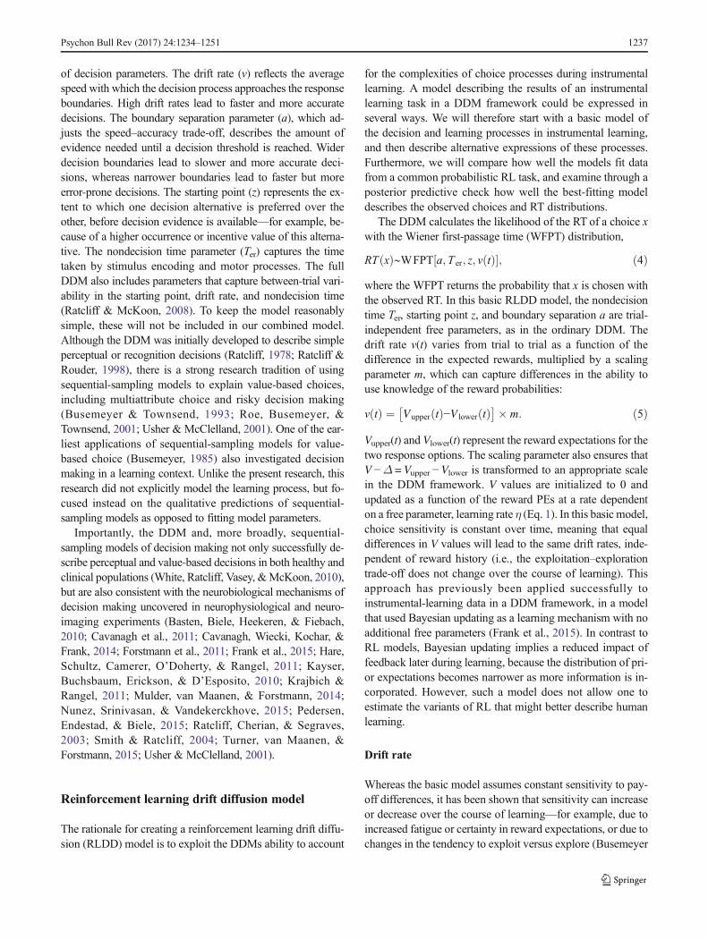
of decision parameters. The drift rate (v) reflects the averagespeed with which the decision process approaches the responseboundaries. High drift rates lead to faster and more accuratedecisions. The boundary separation parameter (a), which ad-justs the speed–accuracy trade-off, describes the amount ofevidence needed until a decision threshold is reached. Widerdecision boundaries lead to slower and more accurate deci-sions, whereas narrower boundaries lead to faster but moreerror-prone decisions. The starting point (z) represents the ex-tent to which one decision alternative is preferred over theother, before decision evidence is available—for example, be-cause of a higher occurrence or incentive value of this alterna-tive. The nondecision time parameter (Ter) captures the timetaken by stimulus encoding and motor processes. The fullDDM also includes parameters that capture between-trial vari-ability in the starting point, drift rate, and nondecision time(Ratcliff & McKoon, 2008). To keep the model reasonablysimple, these will not be included in our combined model.Although the DDM was initially developed to describe simpleperceptual or recognition decisions (Ratcliff, 1978; Ratcliff &Rouder, 1998), there is a strong research tradition of usingsequential-sampling models to explain value-based choices,including multiattribute choice and risky decision making(Busemeyer & Townsend, 1993; Roe, Busemeyer, &Townsend, 2001; Usher & McClelland, 2001). One of the ear-liest applications of sequential-sampling models for value-based choice (Busemeyer, 1985) also investigated decisionmaking in a learning context. Unlike the present research, thisresearch did not explicitly model the learning process, but fo-cused instead on the qualitative predictions of sequential-sampling models as opposed to fitting model parameters.

Importantly, the DDM and, more broadly, sequential-sampling models of decision making not only successfully de-scribe perceptual and value-based decisions in both healthy andclinical populations (White, Ratcliff, Vasey, &McKoon, 2010),but are also consistent with the neurobiological mechanisms ofdecision making uncovered in neurophysiological and neuro-imaging experiments (Basten, Biele, Heekeren, & Fiebach,2010; Cavanagh et al., 2011; Cavanagh, Wiecki, Kochar, &Frank, 2014; Forstmann et al., 2011; Frank et al., 2015; Hare,Schultz, Camerer, O’Doherty, & Rangel, 2011; Kayser,Buchsbaum, Erickson, & D’Esposito, 2010; Krajbich &Rangel, 2011; Mulder, van Maanen, & Forstmann, 2014;Nunez, Srinivasan, & Vandekerckhove, 2015; Pedersen,Endestad, & Biele, 2015; Ratcliff, Cherian, & Segraves,2003; Smith & Ratcliff, 2004; Turner, van Maanen, &Forstmann, 2015; Usher & McClelland, 2001).

Reinforcement learning drift diffusion model

The rationale for creating a reinforcement learning drift diffu-sion (RLDD) model is to exploit the DDMs ability to account

for the complexities of choice processes during instrumentallearning. A model describing the results of an instrumentallearning task in a DDM framework could be expressed inseveral ways. We will therefore start with a basic model ofthe decision and learning processes in instrumental learning,and then describe alternative expressions of these processes.Furthermore, we will compare how well the models fit datafrom a common probabilistic RL task, and examine through aposterior predictive check how well the best-fitting modeldescribes the observed choices and RT distributions.

The DDM calculates the likelihood of the RT of a choice xwith the Wiener first-passage time (WFPT) distribution,

RT xð Þ∼WFPT a; T er; z; v tð Þ½ �; ð4Þwhere the WFPT returns the probability that x is chosen withthe observed RT. In this basic RLDD model, the nondecisiontime Ter, starting point z, and boundary separation a are trial-independent free parameters, as in the ordinary DDM. Thedrift rate v(t) varies from trial to trial as a function of thedifference in the expected rewards, multiplied by a scalingparameter m, which can capture differences in the ability touse knowledge of the reward probabilities:

v tð Þ ¼ Vupper tð Þ−V lower tð Þ� �� m: ð5Þ

Vupper(t) and Vlower(t) represent the reward expectations for thetwo response options. The scaling parameter also ensures thatV −Δ = Vupper − Vlower is transformed to an appropriate scalein the DDM framework. V values are initialized to 0 andupdated as a function of the reward PEs at a rate dependenton a free parameter, learning rate η (Eq. 1). In this basic model,choice sensitivity is constant over time, meaning that equaldifferences in V values will lead to the same drift rates, inde-pendent of reward history (i.e., the exploitation–explorationtrade-off does not change over the course of learning). Thisapproach has previously been applied successfully toinstrumental-learning data in a DDM framework, in a modelthat used Bayesian updating as a learning mechanism with noadditional free parameters (Frank et al., 2015). In contrast toRL models, Bayesian updating implies a reduced impact offeedback later during learning, because the distribution of pri-or expectations becomes narrower as more information is in-corporated. However, such a model does not allow one toestimate the variants of RL that might better describe humanlearning.

Drift rate

Whereas the basic model assumes constant sensitivity to pay-off differences, it has been shown that sensitivity can increaseor decrease over the course of learning—for example, due toincreased fatigue or certainty in reward expectations, or due tochanges in the tendency to exploit versus explore (Busemeyer

Psychon Bull Rev (2017) 24:1234–1251 1237

&Stout, 2002). Accordingly, an extended drift rate calculationallows for additional variability by assuming that themultiplication factor of V-Δ changes according to a powerfunction:

v tð Þ ¼ Vupper−V lower

� �� t=10ð Þp: ð6Þ

In this expression, the drift rate increases throughout learn-ing when the choice consistency parameter p is positive,representing increased confidence in the learned values, anddecreases when p is negative, representing boredom or fatigue.The power function could also account for a move from explo-ration to exploitation when reward sensitivity increases.

Boundary separation

In the basic model described above, the boundary separa-tion (sometimes referred to as the decision threshold) isassumed to be static. However, it could be that the bound-ary separation is altered as learning progresses. Time-dependent changes of decision thresholds could follow apower function by calculating the threshold as a combina-tion of a boundary baseline bb times the boundary powerparameter bp multiplied by trial t:

a tð Þ ¼ bb� t=10ð Þbp: ð7Þ

Learning rate

Several studies have reported differences in updating ofexpected rewards following positive and negative PEs(Gershman, 2015), which is hypothesized to be causedby the differential roles of striatal D1 and D2 dopaminereceptors in separate corticostriatal pathways (Collins &Frank, 2014; Cox, Frank, Larcher, Fellows, & Clark,2015; Frank, Moustafa, Haughey, Curran, & Hutchison,2007). We therefore assumed that V values could bemodeled with asymmetric updating rates, where η+ and η−

are used to update the expected rewards following positiveand negative PEs, respectively.

Model selection

The various mechanisms for drift rate, boundary separation,and learning rate outlined above can be combined into differentmodels, and these models can be compared for their abilities todescribe data. Identifying a model with a good fit requiresseveral considerations (Heathcote, Brown, & Wagenmakers,2015). First of all, a model describing latent cognitive processesneeds to be able to fit data from human or animal experiments.To separate learning from choice sensitivities, we therefore fitmodels on data from subjects performing a probabilistic

instrumental-learning task. To determine which model de-scribed the data best, we first compared models on their relativefits to the data, and then further ascertained the validity of thebest-fitting model by examining its absolute fit (Steingroever,Wetzels, & Wagenmakers, 2014) through posterior predictivechecks (Gelman,Meng, & Stern, 1996). A useful model shouldalso have clearly interpretable parameters, which in turn de-pends on the ability to recover the model parameters—that is,the model must be possible to identify the generative parame-ters. We therefore performed a parameter recovery experimentas a final step to ensure that the fitted parameters described theprocesses that we propose they describe.

Method

Instrumental-learning task

The probabilistic selection task (PST) is an instrumental-learning task that has been used to describe the effect of do-pamine on learning in both clinical and normal populations(Frank, Santamaria, O’Reilly, & Willcutt, 2007; Frank,Seeberger, & O’Reilly, 2004), in which increases in dopamineboost relative learning from positive as compared to negativefeedback. On the basis of a detailed neural-network model ofthe basal ganglia, these effects are thought to be due to theselective modulation of striatal D1 and D2 receptors throughdopamine (Frank et al., 2004). The task has been used toinvestigate the effects of dopamine on learning and decisionmaking in ADHD (Frank, Santamaria, et al., 2007), autismspectrum disorder (Solomon, Frank, & Ragland, 2015),Parkinson’s disease (Frank et al., 2004), and schizophrenia(Doll et al., 2014), among others.

The PST consists of a learning phase and a test phase.During the learning phase, decision makers are presented withthree different stimulus pairs (AB, CD, EF), represented asJapanese hiragana letters, and learn to choose one of the twostimuli in each pair on the basis of reward feedback. Rewardprobabilities differ between the stimulus pairs. In AB trials,choosing A is rewarded with a probability of .8, whereas B isrewarded with a probability of .2. In the CD pair, C isrewarded with a probability of .7, and D .3, and in the EF pair,E is rewarded with a probability of .6, and F .4. Becausestimulus pairs are presented in random order, the reward prob-abilities for all six stimuli have to be maintained throughoutthe task. Success in the learning phase is to learn to maximizerewards by choosing the optimal (A, C, E) over the suboptimal(B, D, F) option in each stimulus pair (AB, CD, EF). Subjectsperform as many blocks (of 60 trials each) as required untiltheir running accuracy at the end of a block is above 65% forAB pairs, 60% for CD pairs, and 50% for EF pairs, or untilthey complete six blocks (360 trials) if the criteria are not met.The PSTalso includes a test phase, which wewill not examine

1238 Psychon Bull Rev (2017) 24:1234–1251

in the present research because it does not involve trial-to-triallearning and exploration. Instead, we will focus on the learn-ing phase of the PST, which can be described as a probabilisticinstrumental-learning task.

The data from the learning phase of the PST in Frank,Santamaria, O’Reilly, and Willcutt (2007) were used to assessthe RLDD models’ abilities to account for data from humansubjects. We also used the task to simulate data from syntheticsubjects in order to test the best-fitting model’s ability to re-cover the parameters. In the original article, the effects ofstimulant medication were tested in ADHD patients with awithin-subjects medication manipulation, and 17 ADHD sub-jects were also compared to 21 healthy controls. In the presentstudy, we focused on the results from ADHD patients to un-derstand the causes of the appreciable effects of medication onthis group. Subjects were tested twice in a within-subjectsdesign. The order of medication administration was random-ized between the ADHD subjects. The results showed thatmedication improved learning performance, and the subse-quent test phase showed that this change was accompaniedby a selective boost in reward learning rather than in learningfrom negative outcomes, consistent with the predictions of thebasal ganglia model related to dopaminergic signaling in stri-atum (Frank, Santamaria, et al., 2007).

Analysis

Parameters in the RLDD models were estimated in a hierar-chical Bayesian framework, in which prior distributions of themodel parameters were updated on the basis of the likelihoodof the data given the model, to yield posterior distributions.The use of Bayesian analysis, and specifically hierarchicalBayesian analysis, has increased in popularity (Craigmile,Peruggia, & Van Zandt, 2010; Lee & Wagenmakers, 2014;Peruggia, Van Zandt, & Chen, 2002; Vandekerckhove,Tuerlinckx, & Lee, 2011; Wetzels, Vandekerckhove,Tuerlinckx, &Wagenmakers, 2010), due to its several benefitsrelative to traditional analysis. First, posterior distributionsdirectly convey the uncertainty associated with parameter es-timates (Gelman et al., 2013; Kruschke, 2010). Second, in ahierarchical approach, individual and group parameters areestimated simultaneously, which ensures mutually constrainedand reliable estimates of both the group and the individualparameters (Gelman et al., 2013; Kruschke, 2010). These ben-efits make a Bayesian hierarchical framework especially valu-able when estimating individual parameters for complexmodels based on a limited amount of data, as is often the casein research with clinical groups (Ahn et al., 2011) or in exper-iments combining parameter estimates with neural data toidentify neural instantiations of proposed processes in cogni-tive models (Cavanagh et al., 2011). In the context of model-ing decision making, Wiecki et al. (2013) showed that a

Bayesian hierarchical approach recovers the parameters ofthe DDM better than do other methods of analysis.

We used the JAGS Wiener module (Wabersich &Vandekerckhove, 2013) in JAGS (Plummer, 2004), via therjags package (Plummer & Stukalov, 2013) in R (RDevelopment Core Team, 2013), to estimate posterior distri-butions. Individual parameters were drawn from the corre-sponding group-level distributions of the baseline (OFF) andmedication effect parameters. Group-level parameters weredrawn from uniformly distributed priors and were estimatedwith noninformative mean and standard deviation grouppriors. For each trial, the likelihood of the RT was assessedby providing the WFPT distribution with the boundary sepa-ration, starting point, nondecision time, and drift rate parame-ters. Responses in the PST data were accuracy-coded, andsymbol–value associations were randomized across subjects.It was therefore assumed that the subjects would not develop abias, represented as a change in starting point (z) toward adecision alternative. To examine whether learning results ina change of the starting point in the direction of the optimalresponse, we compared the RTs for correct and error responsesin the last third of the experiment. Changes in starting pointshould be reflected in slower error RTs (Mulder,Wagenmakers, Ratcliff, Boekel, & Forstmann, 2012; Ratcliff& McKoon, 2008). We focused this analysis on the last thirdof the trials, because in those trials subjects would be morelikely to maximize rewards and less likely to make explorato-ry choices, which more frequently are Berroneous,^ but couldalso be slower for reasons other than bias. Comparison of themedian correct and error RTs showed no clear RT differences,such that the alternative hypothesis was only 1.78 times morelikely than the null-hypothesis (median error RT = 1.039[0.406] s, median correct RT = 0.935 [0.373] s, BF10 = 1.78;Morey & Rouder, 2015). Hierarchical modeling of medianRTs that explicitly accounted for RT differences between theconditions showed the same results, whereas an analysis of alltrials showed even weaker evidence for slower error responses(BF10 = 1.37). The starting point was therefore fixed at .5.Nonresponses (0.011%) and RTs faster than 0.2 s (1.5%) wereremoved prior to analysis.

To capture individual within-subjects effects of medication,we used a dummy variable coding for the medication condi-tion, and estimated for each trial the individual parameters forOFF as a baseline and the individual parameters for ON asbaseline, plus the effect of medication (see The supplementarymaterials for the model code). To assess the effect of medica-tion, we report the posterior means, 95% highest density in-tervals, and Bayes factors as measures of evidence for theexistence of directional effects. Because all priors for groupeffects are symmetric, Bayes factors for directional effects cansimply be calculated as the ratio of the posterior mass abovezero to the posterior mass below zero (Marsman &Wagenmakers, 2016).

Psychon Bull Rev (2017) 24:1234–1251 1239

Relative model fit

Comparison of the relative model fits was performed with anapproximation to the leave-one-out (LOO) cross-validation(Vehtari, Gelman, & Gabry, 2016). In our application, LOOrepeatedly excludes the data from one subject and uses theremaining subjects to predict the data for the left-out subject(i.e., subjects and not trials are independent observations). Ittherefore balances between the likelihood of the data and thecomplexity of the model, because both too-simple and too-complex models would give bad predictions, due to under-and overfitting, respectively. Higher LOO values indicate bet-ter fits. To directly compare the model fits, we computed thedifference in predictive accuracy between models and its stan-dard error, and assumed that the model with the highest pre-dictive ability had a better fit if the 95% confidence interval ofthe difference did not overlap with 0.

Absolute model fit

One should not be encouraged by a relative model comparisonalone (Nassar & Frank, 2016); the best-fitting model of thosedevised might still not capture the key data. The best-fittingmodel from the relative model comparison was therefore eval-uated further to determine its ability to account for key featuresof the data by using measures of absolute model fit, whichinvolves comparing observed results with data generated fromthe estimated parameters. We used two absolute model fitmethods, based on the post-hoc absolute-fit method and thesimulation method described by Steingroever and colleagues(Steingroever et al., 2014). The post-hoc absolute-fit method(also called one-step-ahead prediction) tests a model’s abilityto fit the observed choice patterns given the history of previouschoices, whereas the simulation method tests a model’s abilityto generate the observed choice patterns. We used bothmethods because models that accurately fit observed choicesdo not necessarily accurately generate them (Steingroever et al.,2014). Therefore, a model with a good match to the observedchoice patterns in both methods could, with a higher level ofconfidence, be classified as a good model for describing theunderlying process. The methods were used as posterior pre-dictive checks (Gelman et al., 2013) to identify the model’sability to re-create both the evolution of choice patterns andthe full RT distribution of choices.

In the post-hoc absolute-fit method, parameter value com-binations were sampled from the individuals’ joint posterior.For each trial, observed payoffs were used together with learn-ing parameters to update the expected rewards for the nexttrial. Expected rewards were then used together with decisionparameters to generate choices for the next trial with therwiener function from the RWiener package (Wabersich &Vandekerckhove, 2014). This procedure was performed 100times to account for posterior uncertainty, each time drawing a

parameter combination from a random position in the individ-uals’ joint posterior distribution.

The simulation method followed the same procedure as thepost-hoc absolute-fit method, with the exception that the ex-pected values were updated with payoffs from the simulated,not from the observed, choices. The payoff scheme was thesame as in the PST task, and each synthetic subject made 212choices, which was the average number of trials completed bythe subjects in the PST dataset. We accounted for posterioruncertainty in the simulation method following the same pro-cedure as for the post-hoc absolute-fit method.

Results

Model fit of data from human subjects

Relative model fit

We compared eight models with different expressions of latentprocesses assumed to be involved in reinforcement-based de-cision making, based on data from 17 adult ADHD patients inthe learning phase of the PST task (Frank, Santamaria, et al.,2007). All models were run with four chains with 40,000burn-in samples and 2,000 posterior samples each. To assessconvergence between the Markov chain Monte Carlo

(MCMC) chains, we used the R̂ statistic (Gelman et al.,1996), which measures the degree of variation between chains

relative to the variation within chains. The maximum R̂ valueacross all parameters in all eight models was 1.118 (four pa-rameters in one model above 1.1), indicating that for eachmodel all chains converged successfully (Gelman & Rubin,1992). The LOOwas computed for all models as a measure ofthe relative model fit.

The eight models tested differed in two expressions for cal-culating drift rate variability, two expressions for calculatingboundary separation, and either one or two learning rates (seeTable 1 for descriptions and LOO values for all tested models).All models tested had a better fit than a pure DDM modelassuming no learning processes—that is, with static decisionparameters (Table 1, Supplementary Table 1). The drift rate wascalculated as the difference between expected rewards multi-plied by a scaling parameter, which was either constant (m) orvaried according to a power function (p; see above). The trial-independent scaling models (mean LOO: –16.75) provided onaverage a better fit than the trial-dependent scaling models(mean LOO: –16.805), although this difference was weak (con-fidence interval of the difference: –0.019, 0.128).

Similarly, boundary separation was modeled as a fixed pa-rameter or varied following a power function, changing acrosstrials. The models in which the boundary was trial-dependenthad on average a better fit (mean LOO: –16.573) than the

1240 Psychon Bull Rev (2017) 24:1234–1251

models with fixed boundary separations (mean LOO: –16.983), and this effect was strong (confidence interval ofdifference: 0.172, 0.648). Separating the learning rates forpositive and negative PEs (mean LOO: –16.699) resulted inan overall better fit (confidence interval of difference: 0.052,0.264) than using a single learning rate (mean LOO: –16.857).

Pair-wise comparison of the model fits revealed that twomodels (Models 6 and 8) had a better fit than the other models(see Supplementary Table 1). Themean predictive accuracy ofModel 6 was highest, but it could not be confidently distin-guished from the fit of Model 8. Nevertheless, Model 6 had aslightly better fit (–16.488 vs. –16.506) and had all the prop-erties favored when comparing across models, in that its driftrate was multiplied by a constant scaling factor, the boundaryseparation was estimated to change following a power func-tion, and learning rates were split by the sign of the PE(Table 1). On the basis of these results, we selected Model 6to further investigate how an RLDD model can describe datafrom the learning phase of the PST, and to test its ability torecover parameters from simulated data.

Absolute model fit

The four chains of Model 6 (Table 1) converged for all group-

and individual-level parameters, with R̂ values between 1.00and 1.056 (see https://github.com/gbiele/RLDDM for modelcode and data). There were some dependencies between the

group parameters (Fig. 2), in particular a negative correlationbetween drift rate scaling and the positive learning rate.

Comparing models using estimates of relative model fitsuch as the LOO does not assess whether the modelstested are good models of the data. Absolute model fitprocedures, however, can inform as to whether a modelaccounts for the observed results. A popular approach toestimate absolute model fit is to use posterior predictivechecks (Gelman et al., 2013), which involve comparingthe observed data with data generated on the basis ofposterior parameter distributions. Tests of absolute modelfit for RL models often include a comparison of the evo-lution of choice proportions (learning curves) for observedand predicted data. To validate sequential-sampling modelslike the DDM, however, one usually compares observedand predicted RT distributions. Because the RLLD modelsuse both choices and RTs to estimate parameters, we cre-ated data with both the post-hoc absolute-fit method andthe simulation method procedures described above(Steingroever et al., 2014), and visually compared the sim-ulated data with the observed experimental data on mea-sures of both RT and choice proportion (visual posteriorpredictive check; Gelman & Hill, 2007).

Posterior predictive plots for the development of choiceproportions over time are shown in Fig. 3. For each subject,trials were grouped into bins of ten for each difficulty level.The average choice proportions in each subject’s bins werethen averaged to give the group averages shown in Fig. 3.The leftmost plots display the mean development of observedchoice proportions in favor of the good option from eachdifficulty level for the OFF and ON medication conditions.The middle and rightmost plots display the mean probabilitiesof choosing the good option on the basis of the post-hoc ab-solute-fit method and the simulation method, respectively.The degree of model fit is indicated by the degree to whichthe generated choices resemble the observed choices. Fromvisually inspecting the graphs, it is clear that while ON med-ication, the subjects on average learned to choose the correctoption in all three stimulus pairs, whereas while OFF medica-tion they did not achieve a higher accuracy than about 60% forany of the stimulus pairs. The fitted model recreates this overallpattern: Both methods identify improved performance in theON condition, which is stronger for the more deterministicreward conditions, while also recreating the lack of learningin the OFF group. The model does not recreate the short-termfluctuations in choice proportions, which could reflect othercontributions to trial-to-trial adjustments in this task, outsideof instrumental learning—for example, from working memoryprocesses (Collins & Frank, 2012). Finally, the simulationmethod slightly overestimated the performances in both groups.

The models described here were designed to accountfor underlying processes by incorporating RTs in additionto choices. Therefore, a good model should also be able to

Table 1 Summary of reinforcement-learning drift diffusion models

Model DriftRateScaling

BoundarySeparation

LearningRate

elpd Rank

1 constant fixed single –17.023 7

2 constant power single –16.600 3

3 power fixed single –17.108 8

4 power power single –16.697 4

5 constant fixed dual –16.891 5

6* constant power dual –16.488 1*

7 power fixed dual –16.909 6

8 power power dual –16.506 2

DDM NA fixed NA –17.860 9

In the Drift Rate Scaling column, Bconstant^ indicates that V-delta wasmultiplied by a constant parameter m, whereas Bpower^ indicates that V-delta was multiplied with a parameter p following a power function. ForBoundary Separation, Bfixed^ indicates that boundary separation was atrial-independent free parameter, whereas Bpower^ means that boundaryseparation was estimated with a power function. Under Learning Rate,Bdual^ represents models with separate learning rates for both positiveand negative prediction errors, whereas Bsingle^ models estimate onelearning rate, ignoring the valence of the prediction error. The best-fitting model is marked with an asterisk. elpd = expected log pointwisepredicitive density, NA = not applicable

Psychon Bull Rev (2017) 24:1234–1251 1241

predict the RT distributions of choices. The posterior pre-dictive RTs of choices based on the post-hoc absolute-fitmethod and the simulation method are shown in Fig. 4 asdensities superimposed on histograms of the observed re-sults. Responses in favor of suboptimal options are codedas negative RTs. The results from both the post-hoc abso-lute-fit method and the simulation method re-create theresult that overall accuracy is higher in the easier condi-tions ON medication, while slightly overestimating theproportion of correct trials OFF medication. The tails ofthe distributions are accurately predicted for all difficultylevels for both groups.

Effects of medication on learning and decisionmechanisms

We estimated group and individual parameters dependenton the medication manipulation, both to test whether theresults from the model are in line with the behavioralresults reported by Frank, Santamaria, O’Reilly, andWillcutt (2007) and to examine whether they can contrib-ute to a mechanistic explanation of the processes drivingthe effects of stimulant medication in ADHD (see the

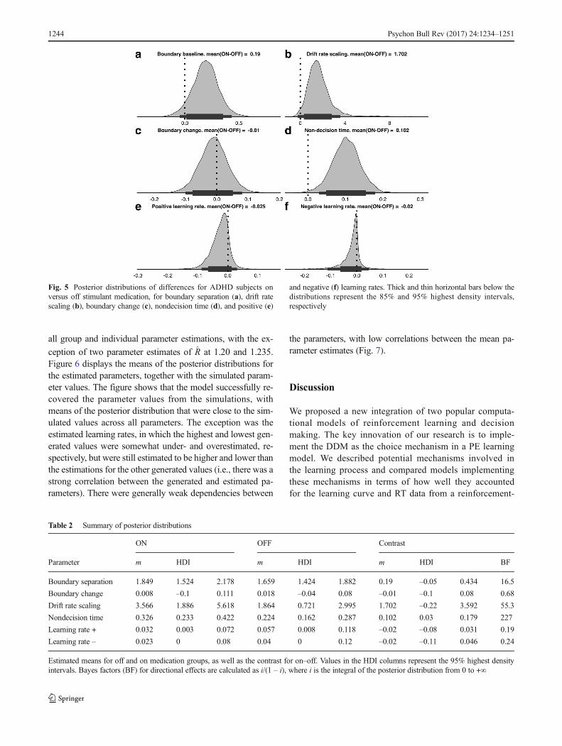
Discussion section). Group-level parameters of thewithin-subjects medication effects were used to assesshow the stimulant medication influenced performance(Fig. 5 and Table 2; Wetzels & Wagenmakers, 2012).

Following Jeffreys’s evidence categories for Bayesfactors (Jeffreys, 1998), the within-subjects comparisonrevealed strong or very strong evidence that medicationincreased the drift rate scaling, nondecision time, andboundary separation (Fig. 5). The results also indicatedsubstantial evidence that medication led to lower posi-tive and negative learning rates.

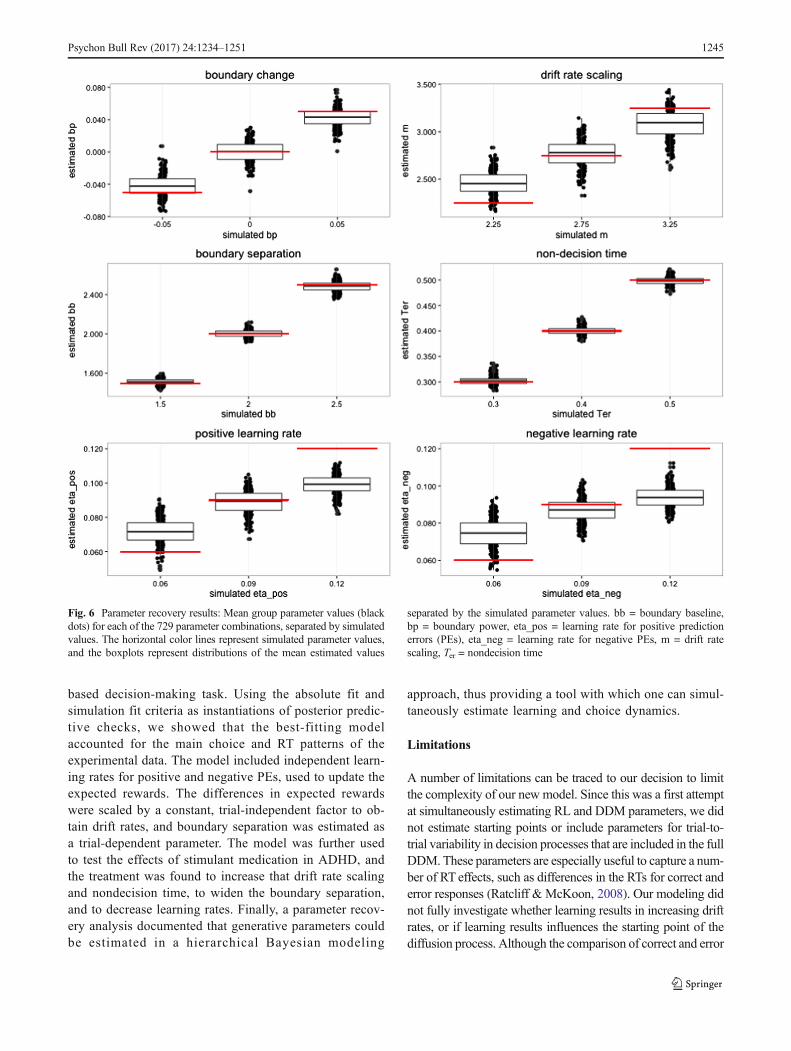
Parameter recovery from simulated data

As a validation of the best-fitting RLDD model (Model 6,Table 1), we performed a parameter recovery study byestimating the posterior distributions of the parameterson simulated data. We used estimated parameter valuesfrom the original PST data to select plausible values forthe free parameters in the best-fitting model. Assigningthree values for each of the six parameters resulted in amatrix with 36 = 729 unique combinations of parametervalues. The choice and RT data were simulated using

Fig. 2 Scatterplot and density of group parameter estimates fromposterior distributions off (red) and on (purple) medication.bb = boundary baseline, bp = boundary power, eta_pos = learning

rate for positive prediction errors (PEs), eta_neg = learning rate fornegative PEs, m = drift rate scaling, Ter = nondecision time

1242 Psychon Bull Rev (2017) 24:1234–1251

assigned parameter values. For each of the 729 combinationsof parameter values, we created data for five synthetic subjectsperforming 212 trials each (the mean number of trialscompleted in the PST dataset).

The model was run with two MCMC chains with 2,000burn-in samples and 2,000 posterior samples for each chain.

The R̂ values for the posterior distributions indicated conver-

gence, with point estimate values of R̂ between 1 and 1.15 for

Fig. 3 Development of mean proportions of choices in favor of theoptimal option for the OFF (top row) and ON (bottom row) medicationgroups, for (a) the observed data, (b) the post-hoc absolute-fit method,and (c) the simulation fit method, across stimulus pairs AB, CD, and EF(see panel legends), which had reward probabilities for the optimal and

suboptimal options of .8–.2, .7–.3, and .6–.4, respectively. The choiceswere fit (b) and simulated (c) by drawing 100 samples from each subject’sposterior distribution. For each subject, trials were grouped into bins often for each difficulty level, and group averages were created from theindividual mean choice proportions for each bin

Fig. 4 Posterior predictive RT distributions across stimulus pairs, shownseparately for the OFF and ON medication groups. Gray histogramsdisplay the observed results, and density lines represent generated

results from the post-hoc absolute-fit method and the simulation fitmethod (in red and purple online, respectively). Choices in favor of thesuboptimal option are coded as negative

Psychon Bull Rev (2017) 24:1234–1251 1243

all group and individual parameter estimations, with the ex-

ception of two parameter estimates of R̂ at 1.20 and 1.235.Figure 6 displays the means of the posterior distributions forthe estimated parameters, together with the simulated param-eter values. The figure shows that the model successfully re-covered the parameter values from the simulations, withmeans of the posterior distribution that were close to the sim-ulated values across all parameters. The exception was theestimated learning rates, in which the highest and lowest gen-erated values were somewhat under- and overestimated, re-spectively, but were still estimated to be higher and lower thanthe estimations for the other generated values (i.e., there was astrong correlation between the generated and estimated pa-rameters). There were generally weak dependencies between

the parameters, with low correlations between the mean pa-rameter estimates (Fig. 7).

Discussion

We proposed a new integration of two popular computa-tional models of reinforcement learning and decisionmaking. The key innovation of our research is to imple-ment the DDM as the choice mechanism in a PE learningmodel. We described potential mechanisms involved inthe learning process and compared models implementingthese mechanisms in terms of how well they accountedfor the learning curve and RT data from a reinforcement-

Fig. 5 Posterior distributions of differences for ADHD subjects onversus off stimulant medication, for boundary separation (a), drift ratescaling (b), boundary change (c), nondecision time (d), and positive (e)

and negative (f) learning rates. Thick and thin horizontal bars below thedistributions represent the 85% and 95% highest density intervals,respectively

Table 2 Summary of posterior distributions

ON OFF Contrast

Parameter m HDI m HDI m HDI BF

Boundary separation 1.849 1.524 2.178 1.659 1.424 1.882 0.19 –0.05 0.434 16.5

Boundary change 0.008 –0.1 0.111 0.018 –0.04 0.08 –0.01 –0.1 0.08 0.68

Drift rate scaling 3.566 1.886 5.618 1.864 0.721 2.995 1.702 –0.22 3.592 55.3

Nondecision time 0.326 0.233 0.422 0.224 0.162 0.287 0.102 0.03 0.179 227

Learning rate + 0.032 0.003 0.072 0.057 0.008 0.118 –0.02 –0.08 0.031 0.19

Learning rate – 0.023 0 0.08 0.04 0 0.12 –0.02 –0.11 0.046 0.24

Estimated means for off and on medication groups, as well as the contrast for on–off. Values in the HDI columns represent the 95% highest densityintervals. Bayes factors (BF) for directional effects are calculated as i/(1 – i), where i is the integral of the posterior distribution from 0 to +∞

1244 Psychon Bull Rev (2017) 24:1234–1251

based decision-making task. Using the absolute fit andsimulation fit criteria as instantiations of posterior predic-tive checks, we showed that the best-fitting modelaccounted for the main choice and RT patterns of theexperimental data. The model included independent learn-ing rates for positive and negative PEs, used to update theexpected rewards. The differences in expected rewardswere scaled by a constant, trial-independent factor to ob-tain drift rates, and boundary separation was estimated asa trial-dependent parameter. The model was further usedto test the effects of stimulant medication in ADHD, andthe treatment was found to increase that drift rate scalingand nondecision time, to widen the boundary separation,and to decrease learning rates. Finally, a parameter recov-ery analysis documented that generative parameters couldbe estimated in a hierarchical Bayesian modeling

approach, thus providing a tool with which one can simul-taneously estimate learning and choice dynamics.

Limitations

A number of limitations can be traced to our decision to limitthe complexity of our new model. Since this was a first attemptat simultaneously estimating RL and DDM parameters, we didnot estimate starting points or include parameters for trial-to-trial variability in decision processes that are included in the fullDDM. These parameters are especially useful to capture a num-ber of RT effects, such as differences in the RTs for correct anderror responses (Ratcliff & McKoon, 2008). Our modeling didnot fully investigate whether learning results in increasing driftrates, or if learning results influences the starting point of thediffusion process. Although the comparison of correct and error

Fig. 6 Parameter recovery results: Mean group parameter values (blackdots) for each of the 729 parameter combinations, separated by simulatedvalues. The horizontal color lines represent simulated parameter values,and the boxplots represent distributions of the mean estimated values

separated by the simulated parameter values. bb = boundary baseline,bp = boundary power, eta_pos = learning rate for positive predictionerrors (PEs), eta_neg = learning rate for negative PEs, m = drift ratescaling, Ter = nondecision time

Psychon Bull Rev (2017) 24:1234–1251 1245

responses revealed very weak evidence for their difference,there was also no clear evidence that they were identical.Hence, further research could explicitly compare models thatassume an influence of learning on the drift rate or startingpoint. In addition, explicitly modeling posterror slowingthrough wider decision boundaries following errors (Dutilhet al., 2012) could have further improved the model fit. Still,these additional parameters are likely not crucial in the contextof the analyzed experiment, because the posterior predictivecheck showed that the model described the RT distribution datawell; for instance, the data did not contain large numbers ofslow responses not captured by the model.

A closer examination of the choice data reveals more roomto improve the modeling. Even though the learning model isalready relatively flexible, it cannot account for all of the choicepatterns. The model tended to overestimate learning success forthe most difficult learning condition, in which both choice op-tions have similar reward probabilities (60:40). Also, whereasthe difference between the proportions of correct responses be-tween learning conditions ON medication was larger at thebeginning of learning than at the end, the model predicted larger

differences at the end. Such patterns could potentially be cap-tured by models with time-varying learning rates (Frank et al.,2015; Krugel et al., 2009; Nassar, Wilson, Heasly, & Gold,2010), by models that could explicitly account for capacity-limited and delay-sensitive working memory in learning(Collins & Frank, 2012), or by more elaborate model-basedapproaches to instrumental learning (Collins & Frank, 2012;Biele, Erev, & Ert, 2009; Doll et al., 2014; Doll, Simon, &Daw, 2012). Hence, whereas the model implements importantfundamental aspects of instrumental learning and decision mak-ing, the implementation of additional processes might be need-ed to fully account for the data from other experiments. Note,though, that increasing the model complexity would typicallymake it more difficult to fit the data, and thus should always beaccompanied by parameter recovery studies that test the inter-pretability of the parameters. As is often seen for RL models,our model did not account for short-time fluctuations in choicebehavior.We suggest that reduced short-time fluctuation in sim-ulated choices can be attributed to the fact that the averagechoice proportions in absolute-fit methods are the result of100 times as many choices as in the original data, which

Fig. 7 Scatterplots and correlations between the mean parameterestimates for each of the 64 parameter combination estimations. bb =boundary baseline, bp = boundary power, eta_pos = learning rate for

positive prediction errors (PEs), eta_neg = learning rate for negativePEs, m = drift rate scaling, Ter = nondecision time

1246 Psychon Bull Rev (2017) 24:1234–1251

effectively reduces variation in the choice proportions betweenbins. By comparison, the overestimation of learning when thechoice options have similar reward probabilities could point to amore systematic failure of the model.

The parameter recovery experiment showed that we wereable to recover the parameter values. Although the resultsshowed that we could recover the precise parameter valuesfor the boundary parameters, nondecision time, and drift ratescaling, it proved hard to recover the high and low learningrates, especially for negative PEs. The fact that it is easier torecover positive learning rates is likely due to the fact thatthere are more trials with positive PEs, as would be expectedin any learning experiment. Still, it should be noted that wewere able to recover the correct order of the learning rateparameters on the group level. Additional parameter recoveryexperiments with only one learning rate for positive and neg-ative PEs resulted in more robust recovery of the learningrates, highlighting the often-observed fact that the price ofincreased model complexity is a less straightforward interpre-tation of the model parameters (results are available uponrequest from the authors). In a nutshell, the parameter recov-ery experiment showed that although we could detect whichgroup had higher learning rates on average, one should notdraw strong conclusions on the basis of small differences be-tween learning rates on the individual level.

Effects of stimulant medication on submechanismsof learning and choice mechanisms in ADHD

We investigated the effects of stimulant medication on learn-ing and decision making (Fig. 5), both to compare these re-sults with the observed results from the original article (Frank,Santamaria, et al., 2007) and to assess the RLDD model’sability to decompose choice patterns into underlying cognitivemechanisms. The original article reported selectiveneuromodulatory effects of dopamine (DA) on go-learningand of noradrenaline (NA) on task switching (Frank,Santamaria, et al., 2007). A comparison of the parameterscould therefore describe the underlying mechanisms drivingthese effects.

Learning rate

The within-subjects effect of stimulant medication identifieddecreased learning rates for positive and negative feedback fol-lowing medication. Although it might at first seem surprisingthat the learning rate was higher off medication, it is importantto note that the faster learning associated with higher learningrates also means greater sensitivity to random fluctuations in thepayoffs.We found a stronger positive correlation between learn-ing rate and accuracy when patients were on as compared to offmedication, selectively for learning rates for positive PEs [inter-action effect: β = 0.84, t(25) = 2.190, p = .038]. These results

show that patients had a more adaptive learning rate onstimulant medication, and also suggest that a reasonablyhigher scaling parameter for differences in reward expec-tation is needed to detect the effects of learning rate onlearning success.

Drift rate scaling

The drift rate parameter in the RLDD model depends on bothlearning rate and sensitivity to reward. The drift rate scalingparameter in our model describes the degree to which currentknowledge is used, as well as the level of exploration versusexploitation. Stimulant medication was found to increase sen-sitivity to reward. These results are in line with the involve-ment of DA in improving the signal-to-noise ratio of corticalrepresentations (Durstewitz, 2006) and striatal filtering of cor-tical input (Nicola, Hopf, & Hjelmstad, 2004), and in main-taining decision values in working memory (Frank,Santamaria, et al., 2007). They are also supported by the op-ponent actor learning model, hypothesizing that DA increasessensitivity to rewards during choice, independently fromlearning (Collins & Frank, 2014).

Boundary separation

Boundary separation estimates increased with medication, in-dicating a shift toward a stronger focus on accuracy in thespeed–accuracy trade-off. This effect is particularly interest-ing, in that it reveals differences in choice processes duringinstrumental learning. It also extends the finding of impairedregulation of the speed–accuracy trade-off during decisionmaking in ADHD (Mulder, Bos, Weusten, & van Belle,2010) to the domain of instrumental learning. The effect canbe related to difficulties with inhibiting responses, in line withthe dual-pathway hypothesis of ADHD (Sonuga-Barke,2003), since responses are given before sufficient evidenceis accumulated. A possible neural explanation of this effectstarts with the recognition that stimulant medication alsomodulates NA levels (Berridge et al., 2006; Devilbiss &Berridge, 2006), which, via the subthalamic nucleus(STN), provides a global Bhold your horses^ signal toprevent premature responding (Cavanagh et al., 2011;Frank, 2006; Frank et al., 2015; Frank, Samanta, Moustafa,& Sherman, 2007; Frank, Scheres, & Sherman, 2007;Ratcliff & Frank, 2012).

Nondecision time

Finally, within-subjects contrasts identified a strong increasein nondecision time through medication, which partially (overand above changes in boundary separation) can explain thefinding of slower RTs in the medicated group (Frank,Santamaria, et al., 2007). Why stimulant medication should

Psychon Bull Rev (2017) 24:1234–1251 1247

affect nondecision time is not immediately clear. However,faster nondecision times in ADHD have been reported in stud-ies comparing DDM parameters on unmedicated childrenwith ADHD and in typically developing controls, with anoverall effect size of 0.32 (95% CI: 0.48–0.15; Karalunas,Geurts, Konrad, Bender, & Nigg, 2014). The studies reportingthis effect could not find a clear interpretation or possiblemechanism driving this change, instead suggesting that itmight be related to motor preparation and not stimulusencoding (Metin et al., 2013). Alternatively, increased com-munication with STN through phasic NA activity could alsoexplain how the STN can suppress premature responses (Aron& Poldrack, 2006).

Implications

Modeling choices during instrumental learning withsequential-sampling models could be useful in several waysto better understand adaptive behavior. One topic of increas-ing interest is response vigor during instrumental learning(see, e.g., Niv, Daw, Joel, & Dayan, 2006). Adaptive learnersadjust their response rates according to the expected averagereward rate, whereby adaptation is thought to depend on DAsignaling (Beierholm et al., 2013). The RLDD model couldinform about response vigor adaptations in several ways. Forexample, average reward expectations in cognitive perceptualtasks can be modeled through PE learning, whereas theadaptation of boundary separation can function as an indica-tor for the adjustment of response vigor. More generally, theadaptive adjustment of response vigor should result inreduced boundary separations over time in instrumental-learning tasks, as well as (crucially) a greater reduction ofboundary separation for decision makers with higher averagereward expectations, which would be indicated by a higherdrift rate. On a psychological level, the joint consideration of(change of) boundary separation and drift rate can help clarifyhow the shift from explorative to exploitative choices,fatigue, or boredom influence decisionmaking in instrumentallearning. In addition to supporting the exploration of basic RLprocesses, the RLDDmodel should also be useful in sheddinglight on cognitive deficiencies of learning and on decisionmaking in clinical groups (Maia & Frank, 2011; Montague,Dolan, Friston, & Dayan, 2012; Ziegler, Pedersen,Mowinckel, & Biele, 2016), as in the effect of stimulantmedication on cognitive processes in ADHD shown here(Fig. 5), but also in other groups with deficient learning anddecision making (Mowinckel, Pedersen, Eilertsen, & Biele,2015), such as in drug addiction (Everitt & Robbins, 2013;Schoenbaum, Roesch, & Stalnaker, 2006), schizophrenia(Doll et al., 2014), and Parkinson’s disease (Frank, Samanta,et al., 2007; Moustafa, Sherman, & Frank, 2008; Yechiam,Busemeyer, Stout, & Bechara, 2005).

References

Ahn, W.-Y., Busemeyer, J. R., Wagenmakers, E.-J., & Stout, J. C.(2008). Comparison of decision learning models using the gen-eralization criterion method. Cognitive Science, 32, 1376–1402. doi:10.1080/03640210802352992

Ahn, W.-Y., Krawitz, A., Kim, W., Busemeyer, J. R., & Brown, J. W.(2011). A model-based fMRI analysis with hierarchical Bayesianparameter estimation. Journal of Neuroscience, Psychology, andEconomics, 4, 95–110. doi:10.1037/a0020684

Aron, A. R., & Poldrack, R. A. (2006). Cortical and subcortical contributionsto stop signal response inhibition: Role of the subthalamic nucleus.Journal of Neuroscience, 26, 2424–2433. doi:10.1523/jneurosci.4682-05.2006

Basten, U., Biele, G., Heekeren, H. R., & Fiebach, C. J. (2010). How thebrain integrates costs and benefits during decision making.Proceedings of the National Academy of Sciences, 107, 21767–21772. doi:10.1073/pnas.0908104107/-/DCSupplemental

Beierholm, U., Guitart-Masip, M., Economides, M., Chowdhury, R., zel,E. D. U., Dolan, R. J., & Dayan, P. (2013). Dopamine modulatesreward-related vigor. Neuropsychopharmacology, 38, 1495–1503.doi:10.1038/npp.2013.48

Berridge, C.W., Devilbiss, D. M., Andrzejewski, M. E., Arnsten, A. F. T.,Kelley, A. E., Schmeichel, B., ... Spencer R. C. (2006).Methylphenidate preferentially increases catecholamine neurotrans-mission within the prefrontal cortex at low doses that enhance cog-nitive function. Biological Psychiatry, 60(10), 1111–1120.doi:10.1016/j.biopsych.2006.04.022

Biele, G., Erev, I., & Ert, E. (2009). Learning, risk attitude and hot stovesin restless bandit problems. Journal of Mathematical Psychology,53(3), 155–167. doi:10.1016/j.jmp.2008.05.006

Bogacz, R., Brown, E., Moehlis, J., Holmes, P., & Cohen, J. D. (2006). Thephysics of optimal decision making: A formal analysis of models ofperformance in two-alternative forced-choice tasks. PsychologicalReview, 113, 700–765. doi:10.1037/0033-295X.113.4.700

Brown, S. D., & Heathcote, A. (2008). The simplest complete model ofchoice response time: Linear ballistic accumulation. CognitivePsychology, 57, 153–178. doi:10.1016/j.cogpsych.2007.12.002

Busemeyer, J. R. (1985). Decision making under uncertainty: A compar-ison of simple scalability, fixed-sample, and sequential-samplingmodels. Journal of Experimental Psychology: Learning, Memory,and Cognition, 11, 538–564. doi:10.1037/0278-7393.11.3.538

Busemeyer, J. R., & Stout, J. C. (2002). A contribution of cognitivedecision models to clinical assessment: Decomposing performanceon the Bechara gambling task. Psychological Assessment, 14, 253–262. doi:10.1037/1040-3590.14.3.253

Busemeyer, J. R., & Townsend, J. T. (1993). Decision field theory: Adynamic-cognitive approach to decision making in an uncertain en-vironment. Psychological Review, 100, 432–459. doi:10.1037/0033-295X.100.3.432

Bush, R. R., & Mosteller, F. (1951). A mathematical model for simplelearning. Psychological Review, 58, 313–323.

Cavanagh, J. F., Wiecki, T. V., Kochar, A., & Frank, M. J. (2014). Eyetracking and pupillometry are indicators of dissociable latent deci-sion processes. Journal of Experimental Psychology: General, 143,1476–1488. doi:10.1037/a0035813

Cavanagh, J. F., Wiecki, T. V., & Cohen, M. X. (2011). Subthalamic nucleusstimulation reverses mediofrontal influence over decision threshold.Nature, 14, 1462–1467. doi:10.1038/nn.2925

Collins, A. G. E., & Frank, M. J. (2012). How much of reinforcementlearning is working memory, not reinforcement learning? A behavioral,computational, and neurogenetic analysis. European Journal ofNeuroscience, 35, 1024–1035. doi:10.1111/j.1460-9568.2011.07980.x

Collins, A. G. E., & Frank, M. J. (2014). Opponent actor learning(OpAL): Modeling interactive effects of striatal dopamine on

1248 Psychon Bull Rev (2017) 24:1234–1251

reinforcement learning and choice incentive. Psychological Review,121, 337–366. doi:10.1037/a0037015

Cox, S., Frank, M. J., Larcher, K., Fellows, L. K., & Clark, C. A. (2015).Striatal D1 and D2 signaling differentially predict learning frompositive and negative outcomes. NeuroImage, 109, 95–101.doi:10.1016/j.neuroimage.2014.12.070

Craigmile, P. F., Peruggia, M., & Van Zandt, T. (2010). HierarchicalBayes models for response time data. Psychometrika, 75, 613–632. doi:10.1007/s11336-010-9172-6

Daw, N. D., O’Doherty, J. P., Dayan, P., Seymour, B., & Dolan, R. J.(2006). Cortical substrates for exploratory decisions in humans.Nature, 441, 876–879. doi:10.1038/nature04766

Devilbiss, D. M., & Berridge, C. W. (2006). Low-dose methylphenidateactions on tonic and phasic locus coeruleus discharge. Journal ofPharmacology and Experimental Therapeutics, 319, 1327–1335.doi:10.1124/jpet.106.110015

Doll, B. B., Simon, D. A., & Daw, N. D. (2012). The ubiquity of model-based reinforcement learning.Current Opinion in Neurobiology, 22,1075–1081. doi:10.1016/j.conb.2012.08.003

Doll, B. B.,Waltz, J. A., Cockburn, J., Brown, J. K., Frank,M. J., &Gold,J. M. (2014). Reduced susceptibility to confirmation bias in schizo-phrenia. Cognitive, Affective, & Behavioral Neuroscience, 14, 715–728. doi:10.3758/s13415-014-0250-6

Durstewitz, D. (2006). A few important points about dopamine’s role inneural network dynamics. Pharmacopsychiatry, 39, 72–75.doi:10.1055/s-2006-931499

Dutilh, G., van Ravenzwaaij, D., Nieuwenhuis, S., van der Maas, H. L. J.,Forstmann, B. U., & Wagenmakers, E.-J. (2012). How to measurepost-error slowing: A confound and a simple solution. Journal ofMathematical Psychology, 56, 208–216. doi:10.1016/j.jmp.2012.04.001

Everitt, B. J., & Robbins, T. W. (2013). From the ventral to the dorsalstriatum: Devolving views of their roles in drug addiction.Neuroscience & Biobehavioral Reviews, 37, 1946–1954.doi:10.1016/j.neubiorev.2013.02.010

Forstmann, B. U., Ratcliff, R., & Wagenmakers, E.-J. (2016). Sequentialsampling models in cognitive neuroscience: Advantages, applica-tions, and extensions. Annual Review of Psychology, 67, 641–666.doi:10.1146/annurev-psych-122414-033645

Forstmann, B. U., Tittgemeyer, M., Wagenmakers, E.-J., Derrfuss,J., Imperati, D., & Brown, S. D. (2011). The speed–accuracytradeoff in the elderly brain: A structural model-based ap-proach. Journal of Neuroscience, 31, 17242–17249.doi:10.1523/JNEUROSCI.0309-11.2011

Forstmann, B. U., & Wagenmakers, E.-J. (Eds.). (2015). An introductionto model-based cognitive neuroscience. New York, NY: Springer.doi:10.1007/978-1-4939-2236-9

Frank, M. J. (2006). Hold your horses: A dynamic computational role forthe subthalamic nucleus in decision making. Neural Networks, 19,1120–1136. doi:10.1016/j.neunet.2006.03.006

Frank, M. J., Gagne, C., Nyhus, E., Masters, S., Wiecki, T. V., Cavanagh, J.F., & Badre, D. (2015). fMRI and EEG predictors of dynamic decisionparameters during human reinforcement learning. Journal ofNeuroscience, 35, 485–494. doi:10.1523/JNEUROSCI.2036-14.2015

Frank, M. J., Moustafa, A. A., Haughey, H. M., Curran, T., & Hutchison, K.E. (2007). Genetic triple dissociation reveals multiple roles for dopa-mine in reinforcement learning. Proceedings of the National Academyof Sciences, 104, 16311–16316. doi:10.1073/pnas.0706111104

Frank, M. J., Samanta, J., Moustafa, A. A., & Sherman, S. J. (2007). Holdyour horses: Impulsivity, deep brain stimulation, and medication inParkinsonism. Science, 318, 1309–1312. doi:10.1126/science.1146157

Frank, M. J., Santamaria, A., O’Reilly, R. C., & Willcutt, E. (2007). Testingcomputational models of dopamine and noradrenaline dysfunction inattention deficit/hyperactivity disorder. Neuropsychopharmacology, 32,1583–1599. doi:10.1038/sj.npp.1301278

Frank, M. J., Scheres, A., & Sherman, S. J. (2007). Understanding decision-making deficits in neurological conditions: Insights from models ofnatural action selection. Philosophical Transactions of the RoyalSociety B, 362, 1641–1654. doi:10.1016/j.braindev.2004.11.009

Frank, M. J., Seeberger, L. C., & O’Reilly, R. C. (2004). By carrot or bystick: Cognitive reinforcement learning in parkinsonism. Science,306, 1940–1943. doi:10.1146/annurev.ento.50.071803.130456

Gelman, A., Carlin, J. B., Stern, H. S., Dunson, D. B., Vehtari, A., &Rubin, D. B. (2013). Bayesian data analysis (3rd ed.). Boca Raton,FL: CRC Press.

Gelman, A., & Hill, J. (2007). Data analysis using regression andmultilevel/hierarchical models. Cambridge, UK: CambridgeUniversity Press.

Gelman, A., Meng, X.-L., & Stern, H. S. (1996). Posterior predictiveassessment of model fitness via realized discrepancies. StatisticaSinica, 6, 733–760.

Gelman, A., & Rubin, D. B. (1992). Inference from iterativesimulation using multiple sequences. Statistical Science, 7,457–472.

Gershman, S. J. (2015). Do learning rates adapt to the distribution ofrewards? Psychonomic Bulletin & Review, 22, 1320–1327.doi:10.3758/s13423-014-0790-3

Glimcher, P. W. (2011). Understanding dopamine and reinforcementlearning: The dopamine reward prediction error hypothesis.Proceedings of the National Academy of Sciences, 108.doi:10.1073/pnas.1014269108

Hare, T. A., Schultz, W., Camerer, C. F., O’Doherty, J. P., &Rangel, A. (2011). Transformation of stimulus value signalsinto motor commands during simple choice. Proceedings ofthe National Academy of Sciences, 108, 18120–18125.doi:10.1073/pnas.1109322108/-/DCSupplemental

Heathcote, A., Brown, S. D., &Wagenmakers, E.-J. (2015). An introduc-tion to good practices in cognitive modeling. In B. U. Forstmann &E.-J. Wagenmakers (Eds.), An introduction to model-based cogni-tive neuroscience (pp. 25–48). New York, NY: Springer.doi:10.1007/978-1-4939-2236-9_2

Jeffreys, H. (1998). The theory of probability. Oxford, UK: OxfordUniversity Press.

Jones, M., & Dzhafarov, E. N. (2014). Unfalsifiability and mutual trans-latability of major modeling schemes for choice reaction time.Psychological Review, 121, 1–32. doi:10.1037/a0034190

Karalunas, S. L., Geurts, H. M., Konrad, K., Bender, S., & Nigg, J. T.(2014). Reaction time variability in ADHD and autism spectrumdisorders: Measurement and mechanisms of a proposed trans-diagnostic phenotype. Journal of Child Psychology andPsychiatry, 55, 685–710. doi:10.1111/jcpp.12217

Kayser, A. S., Buchsbaum, B. R., Erickson, D. T., & D’Esposito, M.(2010). The functional anatomy of a perceptual decision in the hu-man brain. Journal of Neurophysiology, 103, 1179–1194.doi:10.1152/jn.00364.2009

Krajbich, I., & Rangel, A. (2011). Multialternative drift-diffusion model pre-dicts the relationship between visual fixations and choice in value-baseddecisions. Proceedings of the National Academy of Sciences, 108,13852–13857. doi:10.1073/pnas.1101328108/-/DCSupplemental

Krugel, L. K., Biele, G., Mohr, P. N. C., Li, S. C., & Heekeren, H.R. (2009). Genetic variation in dopaminergic neuromodulationinfluences the ability to rapidly and flexibly adapt decisions.Proceedings of the National Academy of Sciences, 106,17951–17956.

Kruschke, J. K. (2010). Doing Bayesian data analysis. San Diego, CA:Academic Press.

Lee, M. D., & Wagenmakers, E.-J. (2014). Bayesian cognitive modeling.Cambridge, UK: Cambridge University Press.

Luce, R. D. (1959). Individual choice behavior: A theoretical analysis.New York; NY: Wiley.

Psychon Bull Rev (2017) 24:1234–1251 1249

Maia, T. V., & Frank, M. J. (2011). From reinforcement learning modelsto psychiatric and neurological disorders. Nature Publishing Group,14, 154–162. doi:10.1038/nn.2723

Marsman, M., & Wagenmakers, E.-J. (2016). Three insights from aBayesian interpretation of the one-sided p value. Educational andPsychological Measurement. doi:10.1177/0013164416669201.Advance online publication.

Metin, B., Roeyers, H.,Wiersema, J. R., van derMeere, J. J., Thompson,M.,& Sonuga-Barke, E. J. S. (2013). ADHD performance reflects ineffi-cient but not impulsive information processing: A diffusionmodel anal-ysis. Neuropsychology, 27, 193–200. doi:10.1037/a0031533

Montague, P. R., Dayan, P., & Sejnowski, T. J. (1996). A framework formesencephalic dopamine systems based on predictive Hebbianlearning. Journal of Neuroscience, 16, 1936–1947.

Montague, P. R., Dolan, R. J., Friston, K. J., & Dayan, P. (2012).Computational psychiatry. Trends in Cognitive Sciences, 16, 72–80. doi:10.1016/j.tics.2011.11.018

Morey, R. D., & Rouder, J. N. (2015). BayesFactor: Computation ofBayes factors for common designs (R package version 0.9.11-1)[Computer software manual]. Retrieved from http://bayesfactorpcl.r-forge.r-project.org

Moustafa, A. A., Sherman, S. J., & Frank, M. J. (2008). A dopaminergicbasis for working memory, learning and attentional shifting inParkinsonism. Neuropsychologia, 46, 3144–3156. doi:10.1016/j.neuropsychologia.2008.07.011

Mowinckel, A. M., Pedersen, M. L., Eilertsen, E., & Biele, G.(2015). A meta-analysis of decision-making and attention inadults with ADHD. Journal of Attention Disorders, 19, 355–367. doi:10.1177/1087054714558872

Mulder, M. J., Bos, D., Weusten, J. M. H., & van Belle, J. (2010). Basicimpairments in regulating the speed–accuracy tradeoff predictsymptoms of attention-deficit/hyperactivity disorder. BiologicalPsychiatry, 68, 1114–1119. doi:10.1016/j.biopsych.2010.07.031

Mulder, M. J., van Maanen, L., & Forstmann, B. U. (2014). Perceptualdecision neurosciences—A model-based review. Neuroscience,277, 872–884. doi:10.1016/j.neuroscience.2014.07.031

Mulder,M. J.,Wagenmakers, E.-J., Ratcliff, R., Boekel,W.,&Forstmann, B.U. (2012). Bias in the brain: A diffusion model analysis of prior prob-ability and potential payoff. Journal of Neuroscience, 32, 2335–2343.doi:10.1523/JNEUROSCI.4156-11.2012

Nassar, M. R., & Frank, M. J. (2016). Taming the beast: Extracting gen-eralizable knowledge from computational models of cognition.Current Opinion in Behavioral Sciences, 11, 49–54. doi:10.1016/j.cobeha.2016.04.003

Nassar, M. R., Wilson, R. C., Heasly, B., & Gold, J. I. (2010). An approx-imately Bayesian delta-rule model explains the dynamics of beliefupdating in a changing environment. Journal of Neuroscience, 30,12366–12378. doi:10.1523/JNEUROSCI.0822-10.2010

Nicola, S. M., Hopf, F. W., & Hjelmstad, G. O. (2004). Contrast enhance-ment: A physiological effect of striatal dopamine? Cell and TissueResearch, 318, 93–106. doi:10.1007/s00441-004-0929-z

Niv, Y., Daw, N. D., Joel, D., & Dayan, P. (2006). Tonic dopamine:Opportunity costs and the control of response vigor.Psychopharmacology, 191, 507–520. doi:10.1007/s00213-006-0502-4

Nunez, M. D., Srinivasan, R., & Vandekerckhove, J. (2015). Individualdifferences in attention influence perceptual decision making.Frontiers in Psychology, 8, 18. doi:10.3389/fpsyg.2015.00018

Pedersen, M. L., Endestad, T., & Biele, G. (2015). Evidence accumula-tion and choice maintenance are dissociated in human perceptualdecision making. PLoS ONE, 10, e140361. doi:10.1371/journal.pone.0140361

Peruggia, M., Van Zandt, T., & Chen, M. (2002). Was it a car or a cat Isaw? An analysis of response times for word recognition. In C.Gatsonis (Ed.), Case studies in Bayesian statistics (Vol. 6, pp.319–334). New York, NY: Springer.

Plummer, M. M. (2004). JAGS: Just another Gibbs sampler [Software].Retrieved from https://sourceforge.net/projects/mcmc-jags/

Plummer, M. M., & Stukalov, A. (2013). Package Brjags.^ [Softwareupdate for JAGS]. Retrieved from https://sourceforge.net/projects/mcmc-jags/

R Development Core Team. (2013). R: A language and environment forstatistical computing. Vienna, Austria: R Foundation for StatisticalComputing. Retrieved from www.R-project.org

Ratcliff, R. (1978). A theory of memory retrieval. Psychological Review,85, 59–108. doi:10.1037/0033-295X.85.2.59

Ratcliff, R., Cherian, A., & Segraves, M. A. (2003). A comparison ofmacaque behavior and superior colliculus neuronal activity to pre-dictions from models of two-choice decisions. Journal ofNeurophysiology, 90, 1392–1407. doi:10.1152/jn.01049.2002

Ratcliff, R., & Frank, M. J. (2012). Reinforcement-based decision mak-ing in cor t icostr iata l ci rcui ts: Mutual constraints byneurocomputational and diffusion models. Neural Computation,24, 1186–1229.

Ratcliff, R., &McKoon, G. (2008). The diffusion decisionmodel: Theoryand data for two-choice decision tasks. Neural Computation, 20,873–922. doi:10.1162/neco.2008.12-06-420

Ratcliff, R., & Rouder, J. N. (1998). Modeling response times fortwo-choice decisions. Psychological Science, 9, 347–356.doi:10.1111/1467-9280.00067

Rescorla, R. A., & Wagner, A. R. (1972). A theory of Pavlovian condi-tioning: Variations in the effectiveness of reinforcement andnonreinforcement. In A. H. Black & W. F. Prokasy (Eds.),Classical conditioning II: Current research and theory (pp. 64–99). New York, NY: Appleton-Century-Crofts.

Roe, R. M., Busemeyer, J. R., & Townsend, J. T. (2001). Multialternativedecision field theory: A dynamic connectionist model of decisionmaking. Psychological Review, 108, 370–392. doi:10.1037/0033-295X.108.2.370

Schoenbaum, G., Roesch, M. R., & Stalnaker, T. A. (2006). Orbitofrontalcortex, decision-making and drug addiction. Trends inNeurosciences, 29, 116–124. doi:10.1016/j.tins.2005.12.006

Schultz, W., Dayan, P., & Montague, P. R. (1997). A neural substrate ofprediction and reward. Science, 275, 1593–1599.

Shadlen, M. N., & Newsome, W. T. (2001). Neural basis of a perceptualdecision in the parietal cortex (area LIP) of the rhesus monkey.Journal of Neurophysiology, 86, 1916–1936.

Smith, P. L., & Ratcliff, R. (2004). Psychology and neurobiology ofsimple decisions. Trends in Neurosciences, 27, 161–168.doi:10.1016/j.tins.2004.01.006

Solomon, M., Frank, M. J., & Ragland, J. D. (2015). Feedback-driventrial-by-trial learning in autism spectrum disorders. AmericanJournal of Psychiatry, 172, 173–181. doi:10.1176/appi.ajp.2014.14010036

Sonuga-Barke, E. J. S. (2003). The dual pathway model of AD/HD: anelaboration of neuro-developmental characteristics. Neuroscience &Biobehavioral Reviews, 27 , 593–604. doi :10.1016/j .neubiorev.2003.08.005

Steingroever, H., Wetzels, R., & Wagenmakers, E.-J. (2014). Absoluteperformance of reinforcement-learning models for the IowaGambling Task. Decision, 1, 161–183. doi:10.1037/dec0000005

Sutton, R. S., & Barto, A. G. (1998). Reinforcement learning. Cambridge,MA: MIT Press.

Turner, B. M., van Maanen, L., & Forstmann, B. U. (2015). Informingcognitive abstractions through neuroimaging: The neural drift diffu-sion model. Psychological Review, 122, 312–336. doi:10.1037/a0038894

Usher, M., & McClelland, J. L. (2001). The time course of perceptualchoice: The leaky, competing accumulator model. PsychologicalReview, 108, 550–592. doi:10.1037/0033-295X.111.3.757

1250 Psychon Bull Rev (2017) 24:1234–1251

Vandekerckhove, J., Tuerlinckx, F., & Lee, M. D. (2011). Hierarchicaldiffusion models for two-choice response times. PsychologicalMethods, 16, 44–62. doi:10.1037/a0021765

Vehtari, A., Gelman, A., & Gabry, J. (2016). Practical Bayesian modelevaluation using leave-one-out cross-validation and WAIC.Retrieved from https://arXiv.org/abs/1507.04544

Wabersich, D., &Vandekerckhove, J. (2013). Extending JAGS:A tutorialon adding custom distributions to JAGS (with a diffusion modelexample). Behavior Research Methods, 46, 15–28. doi:10.3758/s13428-013-0369-3

Wabersich, D., & Vandekerckhove, J. (2014). The RWiener package: AnR package providing distribution functions for the Wiener diffusionmodel. R Journal, 6, 49–56.

Wetzels, R., Vandekerckhove, J., Tuerlinckx, F., & Wagenmakers, E.-J.(2010). Bayesian parameter estimation in the Expectancy Valencemodel of the Iowa gambling task. Journal of MathematicalPsychology, 54, 14–27. doi:10.1016/j.jmp.2008.12.001

Wetzels, R., & Wagenmakers, E.-J. (2012). A default Bayesian hypothesistest for correlations and partial correlations. Psychonomic Bulletin &Review, 19, 1057–1064. doi:10.3758/s13423-012-0295-x

White, C. N., Ratcliff, R., Vasey, M. W., & McKoon, G. (2010). Usingdiffusion models to understand clinical disorders. Journal ofMathematical Psychology, 54, 39–52. doi:10.1016/j.jmp.2010.01.004

Wiecki, T. V., Sofer, I., & Frank, M. J. (2013). HDDM: HierarchicalBayesian estimation of the drift-diffusion model in Python.Frontiers in Neuroinformatics, 7, 14. doi:10.3389/fninf.2013.00014

Yechiam, E., Busemeyer, J. R., Stout, J. C., & Bechara, A. (2005). Usingcognitive models to map relations between neuropsychological dis-orders and human decision-making deficits. Psychological Science,16, 973–978. doi:10.1111/j.1467-9280.2005.01646.x

Ziegler, S., Pedersen, M. L., Mowinckel, A. M., & Biele, G. (2016).Modelling ADHD: a review of ADHD theories through their pre-dictions for computational models of decision-making and rein-forcement learning. Neuroscience & Biobehavioral Reviews.doi:10.1016/j.neubiorev.2016.09.002

Psychon Bull Rev (2017) 24:1234–1251 1251