SEA ICE PHYSICAL PROCESSES AND BlOLOGlCAL LlNKAGES WlTHlN

THE NORTH WATER POLYNYA DURING 1998

BY

C.J. MUNDY

A Thesis Submitted to the Faculty of Graduate Studies

In Partial Fulfillment of the Requirements For the Degree of

MASTER OF ARTS

Deparbnent of Geography University of Manitoba Winnipeg, Manitoba

0 June, 2000

National Library of Canada

Bibliothèque nationale du Canada

Acquisitions and Acquisitions et Bibliographie Services services bibliographiques 395 Wellington Street 395. me Wdliigtm OnawaON KlAON4 Ot\awaON K 1 A W Canada CaMda

The author has granted a non- exclusive Licence ailowing the National Library of Canada to reproduce, loan, distribute or sel1 copies of this thesis in microform, paper or electronic formats.

The author retauis ownership of the copyright in this thesis. Neither the thesis nor substantial extracts fiom it may be printed or otherwise reproduced without the author's permission.

L'auteur a accordé une licence non exclusive permettant à la Bibliothèque nationale du Canada de reproduire, prêter, distribuer ou vendre des copies de cette thèse sous la forme de microfiche/film, de reproduction sur papier ou sur format électronique.

L'auteur conserve la propriété du droit d'auteur qui protège cette thèse. Ni la thèse ni des extraits substantiels de celle-ci ne doivent être imprimés ou autrement reproduits sans son autorisation.

THE UNIVERSITY OF MANITOBA

FACULTY OF CRADUATE STUDIES *****

COPYRIGHT PERMISSION PAGE

Sea Ice Physical Processes and Biological Linkages within the North Water Poiynya During 1998

C. J. Mundy

A Thesis/Practicum submitted to the Faculty of Graduate Studies of The University

of ~Manitoba in partial fulfibnent of the requirements of the degree

of

Master of Arts

Permission has been granted to the Library of The University of Manitoba to lend o r sell copies of this thesis/practicum, to the National Library of Canada to microfilm this thesis/practicum and to lend or sel1 copies of the film, and to Dissertations Abstracts International to publish an abstract of this thesis/practicum.

The author reserves other publication rights, and neither this thesis/prrcticum nor extensive extracts from it may be printed or otherwise reproduced without the author's written permission.

ABSTRACT

Sea ice is a major component of the Earth's climate system and is believed

to be a sensitive indicator of climate change. The North Water (NOW) refers to a

region of anomalous sea ice conditions at the northern end of Baffin Bay. The

dynamic sea ice cover is due to the presence of the NOW polynya. An

explanation for the polynya's occurrence has yet to be confirrned. In this thesis I

studied the spatial and temporal patterns of sea ice cover within the North Water

(NOW) in the context of polynya formation and maintenance mechanisrns.

Further, biological implications of the NOW's sea ice cover patterns were

examined. To accomplish this I developed a sea ice classification scheme for

RADARSAT-1 ScanSAR imagery obtained throughout f 998. 1 extracted sea ice

type and concentration and constructed a Geographic Information System (GIS)

database for analysis of spatial and temporal trends in sea ice cover over this

annual cycle.

Spatially, the results identified a clear and consistent pattern of sea ice cover

throughout 1998. Areas of increased ice deformation (evidenced by the presence

of compressive deforrned ice types) along the east coast of Canada with a fesser

degree of deformation towards Greenland and the Canadian Archipelago were

inferred. Temporally. the polynya opened southward along the Canadian coast

and eastward towards the Greenland coast. Subsequently. the polynya appeared

to be largely controlled by the latent heat mechanism with the exception of the

west Greenland coast. There were some areas of lower ice deformation along

the coast of Greenland that could also be explained, at least in part, through

sensible heat inputs (i.e., both oceanic and atmospheric). These areas of lesser

ice deformation also corresponded to the occurrence of shallow mixed layer

depths earlier than surrounding areas. Consequently, these areas have the

potential to accommodate an earlier primary production bloom.

This thesis represents an advancement in the developrnent of our

understanding of ocean-sea ice-atmosphere processes that occur within the

North Water and its polynya. Links between the polynya's sea ice cover, phys id

mechanisms, biological production and climate variability and change were

made. Further analysis within the NOW Study research network will examine

these links in more detail.

ACKNOWLEDGEMENTS

Reaching the end of a thesis is quite an accomplishment, but it could not be

done alone. There are so many people that I would like to thank. In no particular

order ... I would like to extend my appreciation to Dr. David G. Barber. Your

supervision helped steer me through tough decisions and your "down to earth"

nature and friendship always made you easy to talk to and approach when

dificulties arose. You have placed me in incredible positions and situations that

will continually assist me in my future endeavors and I am very thankful for that. I

look forward to spending at least another year with you as a Research Associate.

Thank you to al1 the residents of rooms 203, 205, 229, 225 and 114 of the

Isbister Building who I know have al1 leant their ears for rny many questions.

More specifically, thank you Johnnies (Yackel, lacoua and Hanesiak) for many

helpful ideas which contributed to this thesis as well as putting up with being

called Johnny. Thank you Ron Hempel, for without you the grid and therefore this

thesis may not have yet been a realization. Thank you roomy (Steve Quiring) for

your much needed assistance during that summer and your never-ending

assistance ever since. Thanks David Mosscrop for al1 the assistance both inside

and outside the lab. Dr. Tim "the namen Papakyriakou. thanks for helping explain

the many faces of energy to me and for boosting my ego at times.

iii

Thank you Dr. Alan J.W. Catchpole and Dr. Gordon G.C. Robinson for your

patience and many suggestions when I fint proposed rny thesis, for critically

reviewing the near final product and for not stumping me too much during my

defense.

I extend my thanks to the Department of Geography, the Centre for Earth

Observation Science (CEOS) and the University of Manitoba who have leant me

the support, facilities, space and tirne required to complete my thesis. Thank you

Trudy Baureiss, Mary Anna, Aggie Roberecki, Suzanne Beaudet, Dr. J. Brierley

and Cr. G. Smith for al1 of the much-needed assistance.

I would like to thank Kathefine Wilson who provided me with great

conversations on our theses topics as well as always being there for me when I

had troubles with the dataset. Thanks Ken Asmus for your unequaled field

preparedness and your bottomless toolbox. While I am in the ballpark. I would

also like to thank the Canadian Ice Service (CIS) for al1 their support.

Thank you Dr. Yves Gratton for providing me with the mixed layer depth data

used in this thesis. I would also like to thank Dr. Peter Minnett for access to the

ship-based meteorological data also used in this thesis.

I extend my appreciation to everyone involved in the International North

Water Polynya Study (NOW) 1998 campaign. including the crew and offcen of

the CCGS Pierre-Raddison. I would like to thank the University of Manitoba for

their support through a Graduate Fellowship. Thanks to the Northern Scientific

Training Program (NSTP) for their field assistance grants. As well. thank you

Polar Continental Shelf Project (PCSP) for your technical and logistical support in

the field.

As many people do. I would like to use a cliché to end this section ... Last.

but certainly not least, I thank my farnily for their support throughout my Masters

degree, the band for helping me chase other goals in rny life. Kate for always

being there for me and ail rny friends.

TABLE OF CONTENTS

ABSTRACT ........................................................................................................................ i

... ACKNO WLEDGEMENTS ............................................................................................... i i i

TABLE OF CONTENTS ................................................................................................... vi

LIST OF FIGURES ........................................................................................................... ix

... LIST OF TABLES ................................................. ,... ................................................... xiii

CHAPTER 1 : INTRODUCTION ..................................................................................... 1

CHAPTER 2: BACKGROUND ..................................................................................... 9

2.1 Sea Ice Types: Evolution and Characteristics ........................................................... 9

2.2 The North Water (NO W) ........................................................................................ 21

2.2.1 The NOW Region ............................................................................................ 21

2.2.2 Recent History of Knowledge on the NOW Polynya Formation and

Maintenance .............................................................................................................. 22

2.2.3 Polynyas and Local Biology ............................................................................ 25

2.2.4 Life within and adjacent to the NOW .............................................................. 29

2.2.5 Sea ice in the NOW ........................... .. ........................................................... 32

2.3 Synthetic Aperture Radar ........................................................................................ 37

2.3.1 SAR Interactions with Sea Ice ......................................................................... 37

2.3.2 The Grey level Co-occurrence Matrix .......................................................... 41

CHAPTER 3: METHODS ............................................................................................. 45

...................................................... 3.1 : The International North Water Polynya Study 45

3 -2 Data ......................................................................................................................... 46

3.2.1 RADARSAT- 1 Data ........................................................................................ 47

3.2.2 Field Data ......................................................................................................... 48

3.2.3 Data Validation ......................................... ... . . . 51

3.3 GIS Framework ............ .. ...................................................................................... 56

3.4 Analytical Design ................ ...... ........................................................................ 59

CHAPTER 4: SCANSAR SEA ICE CLASSIFICATION OF THE NORTH WATER . 63

. . 4.1 Texture Statistics ..................................................................................................... 64

4.2 Classification Procedure ......................................................................................... 69

4.3 Classification Results ............................ ... .......................................................... 72

CHAPTER 5: RESULTS AND DISCUSSION ............................................................... 79

5.1 Sea Ice Spatial Patterns ........................................................................................... 79

5.1 . 1 W inter Period ................................................................................................... 80

5.1 -2 Spring Period ................................................................................................... 86

5.1.3 Fall Period ........................................................................................................ 90

5.2 Sea Ice Temporal Evolution .................................................................................... 95

5.2.1 Prior to Ice Bridge ............................................................................................ 98

5.2.2 Ice Bridge Present ............................................................................................ 99

5.2.3 After Ice Bridge ............................................................................................ 102

5.2 -4 Fall Freeze-up ............................................................................................ 103

5.3 Mixed Layer Depth (MLD) and Sea Ice Patterns ............................................. 103

CHAPTER 6: CONCLUSIONS AND RECOMMENDATIONS ............................... 107

vii

REFERENCES ........................................................................................................ f 15

viii

LIST OF FIGURES

........................................ Figure 1.1. A map of the North Water of northern Baffin Bay. 6

Figure 2.1. Temperature of the density maximum (tpmax) and of the freezing point (tg)

....................... for seawater of different salinities (Afier Weeks and Ackley 1986). 12

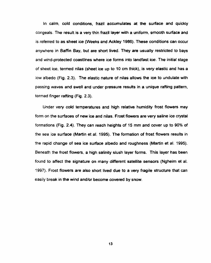
Figure 2.2. Ice core half sections of first-year ice (a) and muitiyear ice (b), demonstrating

basic layers of the ice types. ..................................................................................... 1 2

Figure 2.3. Nilas formed during a period of wind abatement. Top and bottom pictures are

a close-up and horizon view, respectively. Finger rafting is present (examples are

circled) and the beginnings of some fiost flowen (top picture). Picture was taken in

Smith Sound, 1 998. ................................................................................................... 14

Figure 2.4. An icescape of frost flower covered young ice (1 5 cm thick) formed during a

period of cold, calm conditions. Picture was taken in northem Baffin Bay, 1998. .. 15

Figure 2.5. Grease ice forming on the upper right of the image. Dampening of surface

waves has occurred, making the surface appear very smooth. Picture was taken in

Smith Sound, 1998 .................................................................................................... 16

Figure 2.6. Pancake ice formed the day before during high wind conditions. Pictures

were taken in northem Baffin Bay, 1998 (picture on right courtesy of K. Takahashi

and N. Nagao). ...................,...................,... 16

Figure 2.7. The begimings of a young ice sheet formed through the congelation of

pancake ice. Picture was taken as the ship broke through the ice in northern Baffm

Bay, 1 998 (picture courtesy of K. Takahashi and N. Nagao). .................................. 1 7

Figure 2.8. Rubble field formed dong the southem extent of the North Water polynya of

northem Baffin Bay, 1998. ....................................................................................... 19

Figure 2.9. Multiyear ice that had most likely fomcd in the Arctic Basin. Ice thickness

was 2 7 m on top of the hummock. Picture was taken in Wellington Channel, 1997.

.................................................................................................................................. 20

Figure 2.10. Areal concentrations of Chia (mg m-*) in the upper 30 m (Afier Lewis et al.

1 996). ........................................................................................................................ 3 1

Figure 2.1 1. Mean monthly extent of the North Water (After Dunbar 1969). ................ 33

Figure 3.1. Helicopter view of the CCGS Pierre-Raddison. Picture was taken in nonhem

...................................................................................................... Baffin Bay, 1998. 48

Figure 3.2. Pictures of starting a sample site after being craned to the sea ice sampie site

via a metal 'basket' (a) and sampling an ice floe approximately 50 m in diameter (b).

The CCGS Pierre-Raddison is visible in the background of the picture b. Pictures

were taken in northern Baffin Bay, 1 998 (Pictures courtesy of K. Takahashi, N.

Nagao and E. Key). ................................................................................................... 49

Figure 3.3. Photograph of camera and other sensors mounted on the rear of the CCG

helicopter during a grid survey. ................................................................................ 5 1

Figure 3.4. A ScanSAR image sample showing the CCGS Pierre Raddison (arrow

pointing to cluster of bright pixels) in an icescape of nilas ice undemeath the Kane

Basin ice bridge. Date and time of the RADARSAT-1 overpass was Apnl 1 1, 1998

and 2 1 : 1 8 UTC, respectively. .............. . ........................ ...... ...................................... 53

Figure 3 -5 . Surface validated winter ScanSAR imagery (1 28 x 128 pixels) demonstrating

different surface class signatures. Detailed descriptions of windows are provided in

Table 3.2. ............................................................................. . ............................... 55

Figure 3.6. A map of surface validated training and test class sites. ............................... 56

Figure 3.7. A diagrammatic representation of the GIS framework demonstrating: the 2

km grid extent (shaded area) (a), the geo-registered 2krn gnd ceIl (b), a ce11 to

database link (c) and a database to database link (d). ............................................ . 58

Figure 3.8. A 50 km transect of 2 km grid cells used to compare with results obtained in

Steffen (1986). ...................................... ... .............................................................. 61

Figure 4.1. Flow chart of surface type classification scheme. Signature statistics (Mean,

Std. Dev.) for grey level (A) and entropy (B) are provided ................................... ... 76

Figure 5.1. 1998 winter period (Jan. 2 1 through Feb. 28) k-means cluster results for the

GIS grid. The table provides the mean surface type composition for each blue-

shaded cluster. ........................................................................................................... 8 1

Figure 5.2. Averaged 1998 winter period (Jan. 2 1 through Feb. 28) concentrations of

multiyear (a) and rubble (b) sea ice types. .............. ...................................... . . . 82

Figure 5.3. 1998 spring period (Mar. 1 7 through May 26) k-means cluster results for the

GIS grid. The table provides the mean surface type composition for each blue-

shaded cluster. ......................................................... .............................................. 87

Figure 5.4. Averaged 1998 spring period (Mar. 17 through May 26) concentrations of

rubble sea ice (a) and open water (b). .................................................................. 88

Figure 5.5. 1998 fa11 period (Oct. 15 through Dec. 7) k-means cluster results for the GIS

grid. The table provides the mean surface type composition for each blue-shaded

cluster. ....................................................................................................................... 9 1

Figure 5.6. Averaged 1998 fa11 period (Oct. 15 through Dec. 7) concentrations of open

water (a) and medium first-year sea ice (b). ........................................................... 93

Figure 5.7. Map of the North Water sub-regions. ............................................................ 95

Figure 5.8. Sea ice concentration time series during 1998 for CA1 (a), GL I (b), CA2 (c),

GL2 (d), CA3 (e), GL3 (f), CA4 (g) and GL4 (h). 1, II, III and N depict the four

temporal stages outlined in the text. ......................................................................... 97

Figure 5.9. Sea ice concentration time series during 1998 for CA5 (a). GLS W (b), CA6

(c), GL6W (d), GLSE (e) and GL5E (0. 1, II, III and IV depict the four temporal

stages outlined in the text .......................................................................................... 98

Figure 5.10. Meteorological variables including wind speed (Wind Sp.), wind direction

(Wind Dir.), air temperature (Air T), relative humidity (RH), incident short wave

(S W) and long wave energy (LW) and pressure (P) collected in transit on board the

CCGS Pierre Raddison during the 1998 North Water Polynya Study Expedition

(Afier Mimett 2000). Vertical dashed lines were added to highlight the month of

May (Day of Year 121 to 151) ................................................................................ 101

Figure 5.1 1. Mixed layer depths (m) for CTD casts made during Legs 1 (March 26 to

May 5 (a)), 2 (May 5 to June 2 (b)), 3 (June 2 to June 29 (c)) and 4 (June 29 to July

27 (d)) of the 1998 International North Water Polynya Study expedition.

Interpolated 10 km radii swround each CTD cast location. ................................... 105

xii

LIST OF TABLES

Table 3.1. Validated surface types for RADARSAT- 1 ScanSAR wide beam mode

imagery. ....................-....*............. .......... ............................. - ..................................... 54

Table 3.2. Window descriptions for Fig. 2. .................... - ...-... . ..................................... 55

Table 4.1. Contingency table of percent agreement between classified and training data,

obtained from the initial Multiple Discriminate Analysis (MDA) results. ............... 72

Table 4.2. Correlation of discriminating variables with canonical discriminate functions,

obtained from final MDA results. ..................................................................... . 74

Table 4.3. Kappa coefficients (K) and standard deviations (K,) for combinations of

discriminating variables based on Table 4.2 results. ........................................... 75

Table 5.1. Surface type composition along a 50 km transect for the winter, spring ad

fa11 periods of 1998 (Jan.21 through Feb. 28, Mar. 17 through May 26 and Oct. 15

through Dec. 7, respectively). ............................................................................. . . 85

xiii

CHAPTER 1: INTRODUCTION

The Earth's clirnate - a complex interaction between incoming solar

radiation, emitted Earth radiation and the characteristics of the planet's surface

and atmosphere - has been ever-changing throughout its history. However,

increased atmospheric COz levels and a cfimate warming over the past century

have raised public concern. A question of whether this change has an

anthropogenic origin or is simply the natural variability of the Earth's climate has

been posed (World Climate Research Program (WCRP) objective - in McBean

1992). In order to answer this question we must first be able to detect and

understand change in relation to the physical interactions causing the change.

Throughout the last couple of decades climate change research has largely

focused on polar regions where 1 is thought the change will occur earlier and will

likely be amplified relative to temperate and tropical regions of the planet (e.g.,

Barry et al. 1993).

Due to the many difficulties associated with research in polar regions (Le.,

low temperatures, inaccessibility, 24 hr winter darkness and high logistical

expenses), polar marine systems have remained poorly understood relative to

other regions of the planet. However, their sensitivity to climate variability,

importance to many biological species and profound influence on ocean

circulation and global climate are well recognized. One of the most unique and

vital components of these regions is a temporally and spatially dynamic sea ice

cover.

Sea ice: (i) influences global ocean thennohaline circulation by supplying

cold, dense brine through accretion (freeze-up) and fresh surface water through

ablation (melt) (Aagaard and Carmack 1989); (ii) provides a platfonn for

deposition of snow, which in combination control the ocean-sea ice-atmosphere

(OSA) exchange of mass, heat and rnomentum (Maykut 1978; 1982) and affect

the surface radiation balance through changes in albedo (Barry et al. 1993); and

(iii) has both direct and indirect consequences on biological production (e-g.,

Welch et al. 1992). Furthemore, sea ice has been hypothesized as a sensitive

indicator of climate change through possible feedback mechanisms operating

across the OSA interface (Barry et al. 1993). Mounting evidence of climate

change includes temporal trends of decreasing Arctic pack-ice extent (e.g.,

Parkinson et al. 1999) and thickness (e-g., Rothrock et al. 1999).

Sea ice is both spatially and temporally variable. Over an annual cycle, the

ocean's ice cover profoundly modifies up to 15% of the Earth's surface. Advance

and retreat of sea ice cause most of this change. Parkinson et al. (1999) found

the Arctic average seasonal coverage (1978-1996) of sea ice extents to range

from a minimum of 7.0 x 1 o6 km2 in Septernber to a maximum of 15.4 x 106 km2

in March. Interannual variations among these averages are quite substantial with

regional oscillations demonstrating an approximate ten-year cycle (Mysak and

Venegas 1998).

Throughout the winter months, the extensive Arctic sea ice cover is dotted

with anornalous openings referred to as polynyas and leads. Modeled and

observed results have dernonstrated new ice ( ~ 3 0 cm) and open water to only

cover 1% (Thorndike et al. 1975) to 2.6% (Mclaren 1988) of the total Arctic

Ocean during this time. However. heat exchange through open water and new

ice surfaces can be two orden of magnitude greater than surrounding snow

covered sea ice (Maykut 1978). Consequently, polynyas and leads dominate

regional heat budgets (Maykut 1978) and significantly influence salt flux to the

oceans (Canack 1990) and heat flux to the atmosphere in winter (Maykut 1982).

Polynyas and leads have been distinguished through definitions set forth by

the World Meteorological Organization's official glossary (WMO 1970). A lead is

a linear feature, which occurs due to ice divergence along weak points in the ice.

A polynya is defined as any nonlinear-shaped area of open water and/or sea ice

cover < 30 cm thick enclosed by a much thicker ice cover (WMO 1970). It can be

restricted on one side by a coast, terrned shore polynyas, or bounded by fast ice,

termed flaw polynyas. Polynyas that occur in the same position every year are

called recurring polynyas (WMO 1970). The latter type can also be subdivided

into: those which remain open throughout winter and those which can freeze over

during the coldest months, yet open in late winter or early spring. In contrast to

leads, which form and freeze over periodically (e.g., c 1 day; Bauer and Martin

1983). polynyas, once forrned, generally remain open until the surrounding ice

cover breaks-up.

Two generalized mechanisms, termed latent and sensible heat, act to fomi

and rnaintain polynyas (Smith et al. 1990). A latent heat mechanism involves

wind andlor current driven divergence of ice (along a coast, ice shelf, grounded

ice berg or landfast ice structure) with the latent heat of fusion, released from

continual ice accretion, balancing heat loss to the atmosphere and hence

maintaining open water. A polynya formed under this type of mechanism is

expected to be associated with high ice defomation (Le., ice defomation caused

through surface turbulence). Aitematively, a sensible heat mechanism impedes

the formation of ice through a w a m oceanic heat input and would therefore be

less likely associated with high ice deformation. Due to a polynya's dependence

on atmospheric and oceanic processes affecting its sea ice cover. the

significance of a polynya is strongly linked to the significance of sea ice.

Consequently, polynyas are thought to be sensitive to climatic change (IAPP

1989).

The presence of recurring polynyas in the Arctic makes them important to al1

biolog ical life (Stirling 1 980, 1997; Massom 1988) including indigenous peoples

(Schledermann 1980). They provide overwintering areas for many marine

mammal species including : polar bears (Ursus mantirnus). ringed seals (Phoca

hispida), bearded seals (Elignathus barbatus), walruses (Odobenus rosmarus),

belug a (white) whales (Delphinapterus leucas), nawhals (Monodon monoceros)

and bowhead (Greenland Right) whales (Balaena mystiscetus) (e-g.. Stirling

1980, 1997; Finley and Renaud 1980). In the spring, they can account for early

and enhanced primary production blooms (e.g.. Lewis et al. 1996), which provide

food for higher trophic level feeders (Welch et al. 1992). Subsequently, polynyas

are important to early spring migrations for al1 of the mammal species mentioned

above and many seabird species. Some of the more prominent seabird species

include: dovekies (Alle alle), thick-billed murres (Uria lomvia), black guillemotts

(Cepphus grille), black-legged kittiwakes (Rissa tndactyla) , ivory g ulls (Pagophila

ebumean), glaucous gulls (Lams hypedwreus) and northern fulmars (Fulmans

glacialis) (Nettleship and Evans 1 985).

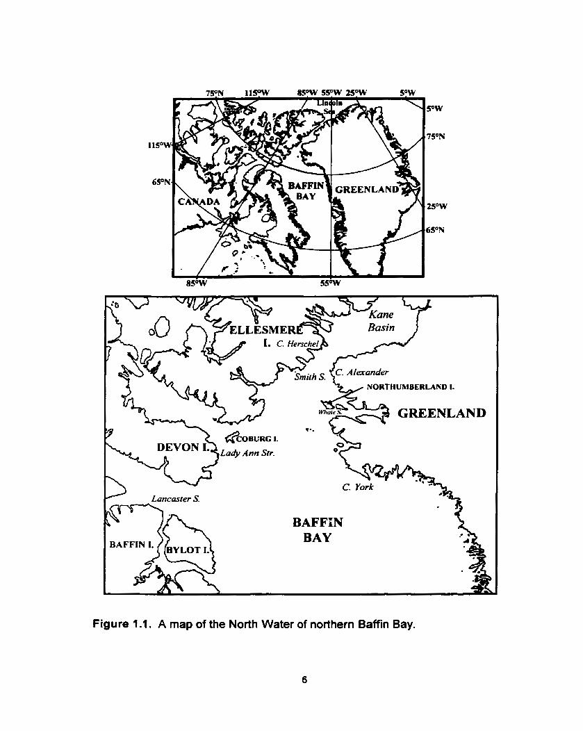
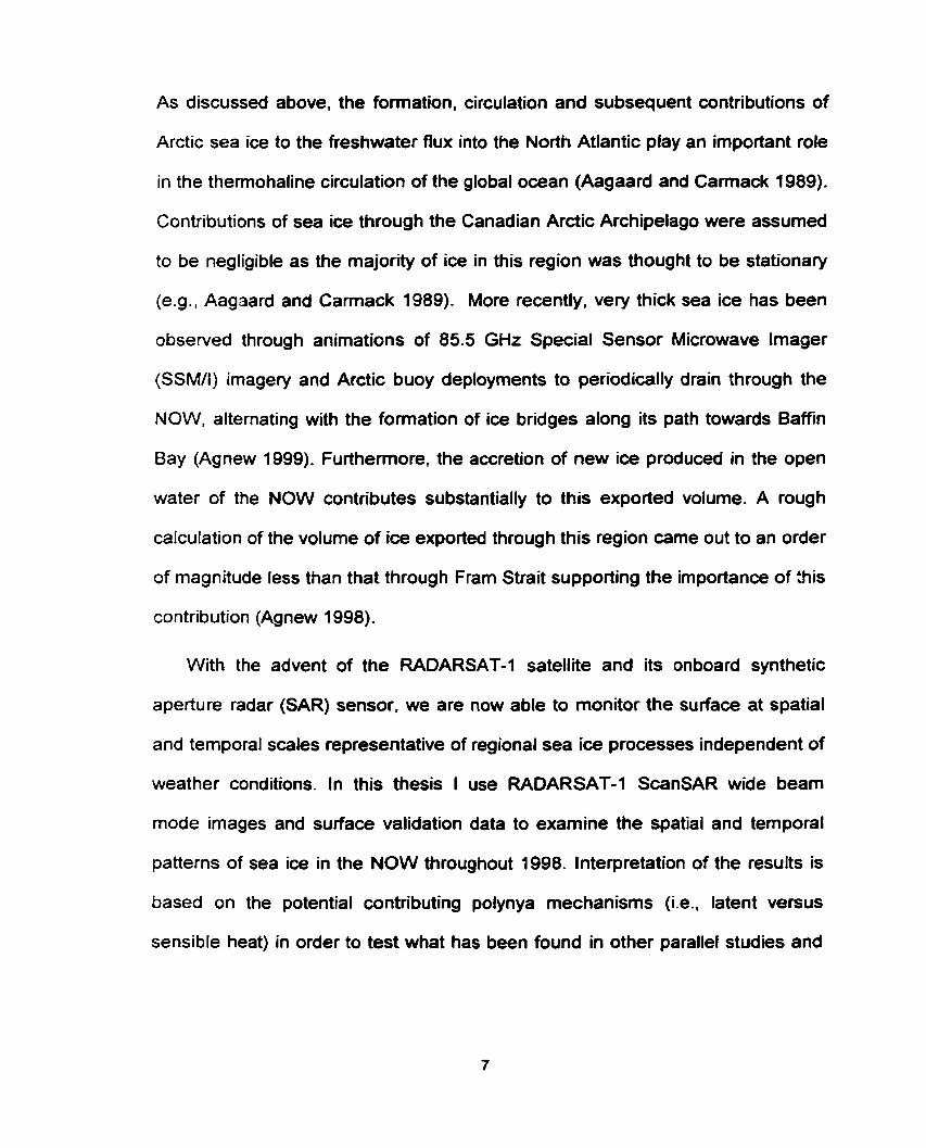
The North Water (NOW) refers to a region of anomalous sea ice cover in

northern Baffin Bay (Fig. 1.1). It encompasses both Canadian and Greenland

waters (Fig. 1 .l). which makes the region of international interest. Further, it is

home to the largest recurring polynya found in the Canadian Archipelago. The

NOW polynya has also been acknowledged as perhaps the most biologically

significant polynya in the Canadian Arctic due in part to its size and permanence

(Stirling 1980; 1997). Consequently, the NOW has drawn attention from a

multitude of different acadernic fields including circumpolar specialists from bath

the physical and social sciences. Of particular interest to researchers are the

physical mechanisms that act to form and maintain the polynya and their

relationship to climate change and local biology.

BAFFIN BAY

Figure 7 .l. A map of the North Water of northern Baffin Bay.

As discussed above, the formation, circulation and subsequent contributions of

Arctic sea ice to the freshwater fiux into the North Atlantic play an important role

in the thermohaline circulation of the global ocean (Aagaard and Camack 1989).

Contributions of sea ice through the Canadian Arctic Archipelago were assumed

to be negligible as the majority of ice in this region was thought to be stationary

(e.g., Aagaard and Carmack 1989). More recently, very thick sea ice has been

observed through animations of 85.5 GHz Special Sensor Microwave Imager

(SSMII) imager- and Arctic buoy deployments to periodically drain through the

NOW, alternating with the formation of ice bridges along its path towards Baffin

Bay (Agnew 1999). Furtherrnore, the accretion of new ice produced in the open

water of the NOW contributes substantially to this exported volume. A rough

calculation of the volume of ice exported through this region came out to an order

of magnitude less than that through Fram Strait supporting the importance of 31is

contribution (Agnew 1998).

With the advent of the RADARSAT-1 satellite and its onboard synthetic

aperture radar (SAR) sensor. we are now able to monitor the surface at spatial

and temporal scales representative of regional sea ice processes independent of

weather conditions. In this thesis I use RADARSAT-1 ScanSAR wide beam

mode images and surface validation data to examine the spatial and temporal

patterns of sea ice in the NOW throughout 1998. lnterpretation of the results is

based on the potential contributing polynya mechanisms (Le., latent versus

sensible heat) in order to test what has been found in other parallel studies and

provide insight where data collection has been lacking. Further, biological

implications of the North Water's sea ice cover patterns are examined.

More specifically, the main objectives of this thesis are: (1) to develop a

robust ScanSAR sea ice classification scheme; (2) to examine the spatial and

temporal patterns of sea ice cover within the North Water (NOW) in relation to

the potential physical mechanisms responsible for the NOW polynya's

occurrence, and (3) ta relate the sea iœ spatio-temporal patterns to the potential

for biological productivity within the NOW.

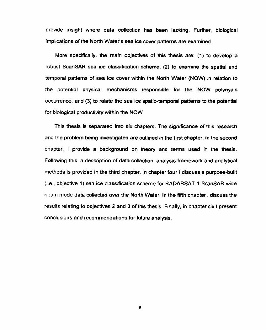
This thesis is separated into six chapters. The signifieance of this research

and the problem being investigated are outlined in the first chapter. In the second

chapter, 1 provide a background on theory and ternis used in the thesis.

Following this, a description of data collection, analysis framework and analytical

methods is provided in the third chapter. In chapter four I discuss a purpose-built

(Le., objective 1) sea ice classification scheme for RADARSAT-1 ScanSAR wide

beam mode data collected over the North Water. In the fifth chapter I discuss the

results relating to objectives 2 and 3 of this thesis. Finally, in chapter six I present

conclusions and recommendations for future analysis.

CHAPTER 2: BACKGROUND

In this chapter I provide an overview of sea ice, the North Water and

Synthetic Aperture Radar (SAR), segmented into 3 sections. The first section

describes the evolution and subsequent charateristics of sea ice. In section two I

examine our current knowledge pertaining to the North Water (NOW). In the final

section I describe the basic theory of Synthetic Aperture Radar (SAR) data in

relation to remote sensing of sea ice. In particular I introduce the Grey Level Co-

occurrence Matrix (GLCM) as a tool in separating various ice types frorn SAR

imagery.

2.1 Sea /ce Types: Evolution and Characteristics

Since the 1970's. sea ice has been extensively studied as it is thought to be

a sensitive indicator of climate change (Barry et al. 1993) and plays an active role

in the global climate (e.g.. Aagaard and Cannack 1989). This section describes

the evolution of sea ice types in differing environments and subsequent

characteristics including some key definitions that will be used throughout this

thesis'.

Sea ice is defined as any form of ice found within the ocean that has

originated from the freezing of seawater (WMO 1970). Seawater is a combination

of pure water and various dissolved solids (salts) and gases with an approximate

salinity of 35%0. It should be noted that ocean salinity varies greatly between

water masses. particularly at polar latitudes (Carmack 1990). The formation of

ice from seawater is a complex process where the salt and gas components are

squeezed out and trapped within as the pure water component creates hydrogen

bonds forming ctystals of ice. The result is a mixture of ice, brine (a concentrated

salt-water mixture), solid salts (if temperatures are cold enough) and gas (Weeks

and Ackley 1986).

Based on mobility, sea ice is distinguished as either fast ice or pack ice. Fast

ice refers to ice that is fastened to land and is therefore immobile. It may fom in-

situ or by freezing of free-fioating ice to the shore or fast ice edge. Alternatively.

pack ice refers to mobile ice or any f o n of ice that is not fast ice.

Temporally, sea ice develops through the following chronological stages: (i)

new ice. (ii) nilas, (iii) young ice, (iv) first-year ice and (v) old or multiyear ice.

New ice refers to very thin ice forrns that are a collection of individual crystals not

completely frozen together. Nilas and young ice are transition stages based on

ice thickness and crystal structure. First-year ice refen to ice developed from

1 General terrninology of sea ice used this thesis is based on mobility, ageithickness and fom; however the definitions by no means encapsulate al1 types of sea ice that have been delineated. For a complete synthesis, please refer to WMO (1970) and/or MANICE (1994).

10

young ice that is not more than one winter's growth. Old ice has been split up

into second-year ice (survived only one summer's melt) and multiyear ice

(survived at least two summers' melt) by the WMO (1970). However, most

scientific literature uses the terni "multiyear" ice in reference to both old ice types

(e-g., Weeks and Ackley 1986). 1 will use the latter reference in that 'multiyeaf

ice will refer to ice that has survived at least one summer's melt. Throughout this

temporal development sea ice can demonstrate numerous forms and features

depending on environmental conditions. These developed forms and features are

the basis for further sea ice distinction.

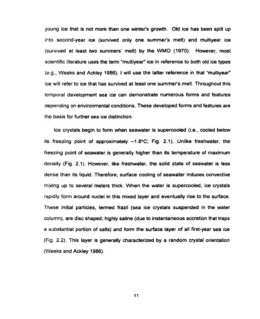
Ice crystals begin to fonn when seawater is supercooled (Le., cooled below

its freezing point of approximately -1.8OC; Fig. 2.1). Unlike freshwater, the

freezing point of seawater is generally higher than its temperature of maximum

density (Fig. 2.1). However, like freshwater, the solid state of seawater is less

dense than its liquid. Therefore, surface cooling of seawater induces convective

rnixing up to several meters thick. When the water is supercooled, ice crystals

rapidly f om around nuclei in this mixed layer and eventually rise to the surface.

These initial particles, tened frazil (sea ice crystals suspended in the water

column), are disc shaped, highly saline (due to instantaneous accretion that traps

a substantial portion of salts) and fom the surface layer of al1 first-year sea ice

(Fig. 2.2). This layer is generally characterized by a random crystal orientation

(Weeks and Ackley 1986).

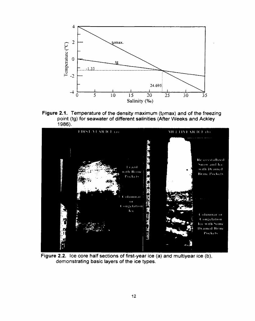
Figure 2.2. Ice core half sections of first-year ice (a) and multiyear ice (b), demonstrating basic layers of the ice types.

In calm, cold conditions, frazil accumulates at the surface and quickly

congeals. The result is a very thin frazil layer with a uniforni, smooth surface and

is referred to as sheet ice (Weeks and Ackley 1986). These conditions can occur

anywhere in Baffm Bay, but are short lived. They are usually restricted to bays

and wind-protected coastlines where ice foms into landfast ice. The initial stage

of sheet ice, termed nilas (sheet ice up to 10 cm thick), is very elastic and has a

low albedo (Fig. 2.3). The elastic nature of nilas allows the ice to undulate with

passing waves and swell and under pressure results in a unique rafting pattern,

termed finger rafting (Fig. 2.3).

Under very cold temperatures and high relative humidity frost flowers may

form on the surfaces of new ice and nilas. Frost flowers are very saline ice crystal

formations (Fig. 2.4). They can reach heights of 15 mm and cover up to 90% of

the sea ice surface (Martin et al. 1995). The formation of frost flowers results in

the rapid change of sea ice surface albedo and roughness (Martin et al. 1995).

Beneath the frost flowen, a high salinity slush layer foms. This layer has been

found to affect the signature on many different satellite sensors (Ngheim et al.

1997). Frost flowers are also short lived due to a very fragile structure that can

easily break in the wind andfor become covered by snow.

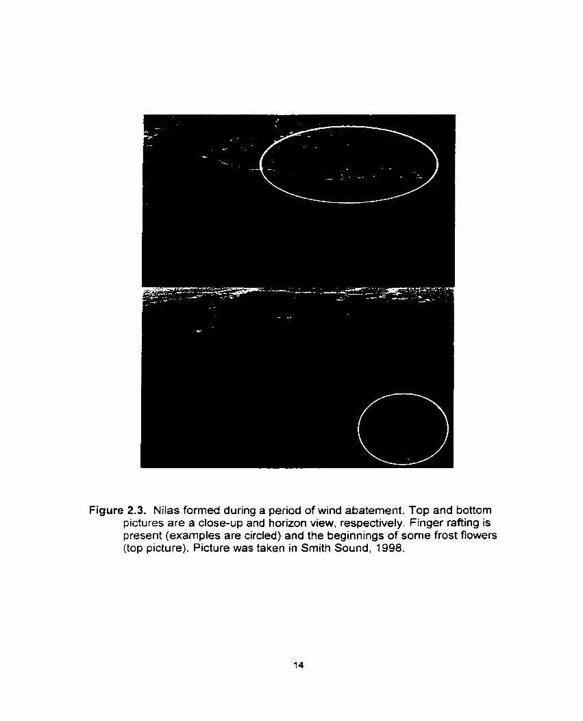
Figure 2.3. Nilas formed during a period of wind abatement. Top and bottom pictures are a close-up and horizon view, respectively. Finger rafting is present (examples are circled) and the beginnings of some frost flowers (top picture). Picture was taken in Smith Sound, 1998.

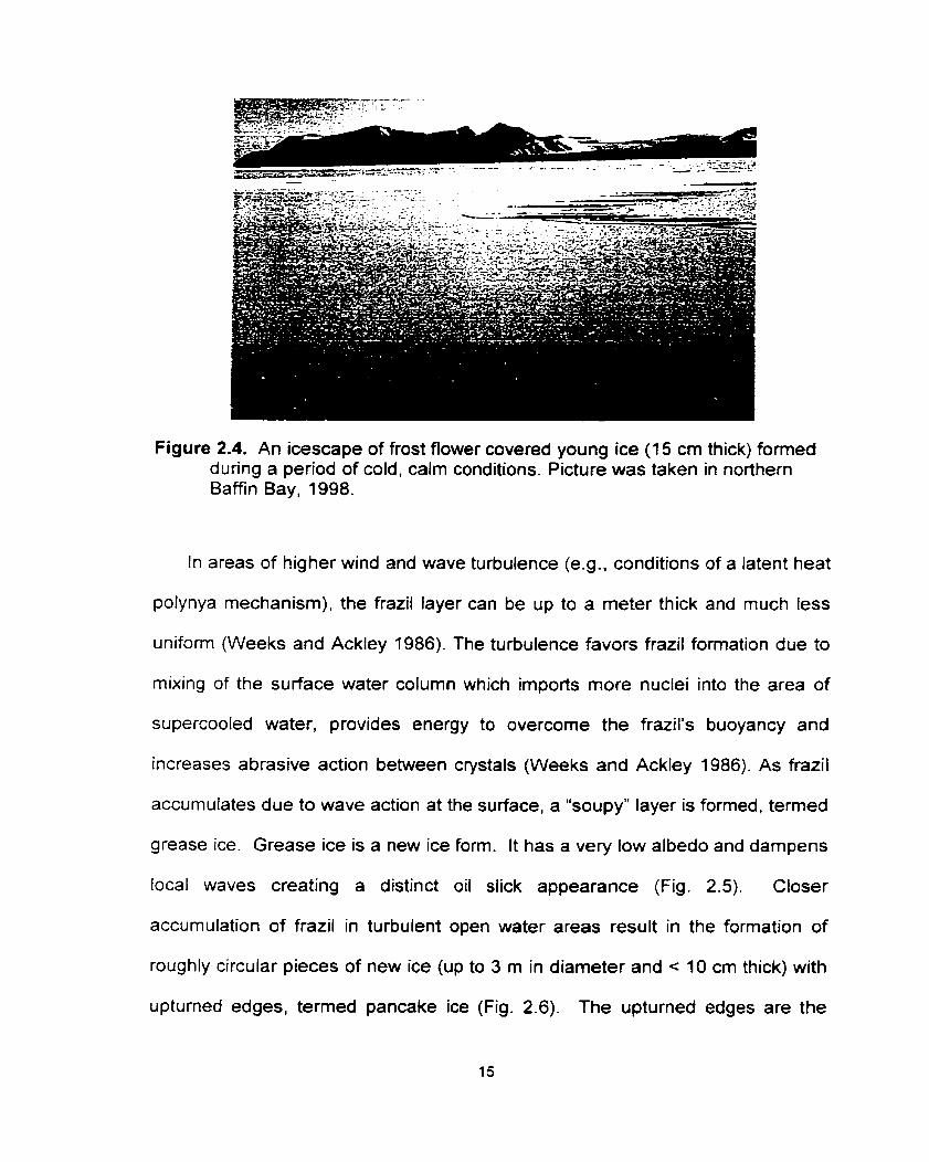
Figure 2.4. An icescape of frost flower covered young ice (1 5 cm thick) formed during a period of cold, calm conditions. Picture was taken in northern Baffin Bay, 1998.

In areas of higher wind and wave turbulence (e-g., conditions of a latent heat

polynya mechanism), the frazil layer can be up to a meter thick and much less

uniform (Weeks and Ackley 1986). The turbulence favors frazil formation due to

mixing of the surface water column which imports more nuclei into the area of

supercooled water, provides energy to overcorne the frazil's buoyancy and

increases abrasive action between crystals (Weeks and Ackley 1986). As frazil

accumuiates due to wave action at the surface, a "soupy" layer is formed, termed

grease ice. Grease ice is a new ice form. It has a very low albedo and dampens

local waves creating a distinct oil slick appearance (Fig. 2.5). Closer

accumulation of frazil in turbulent open water areas result in the formation of

roughly circular pieces of new ice (up to 3 m in diameter and c 10 cm thick) with

upturned edges, termed pancake ice (Fig. 2.6). The upturned edges are the

result of wave action, which cause repeated convergence and divergence

between neighboring pieces of ice. The repeated contacts create the circular

form and push frazil ont0 the edge of the pancake (Weeks and Ackley 1986).

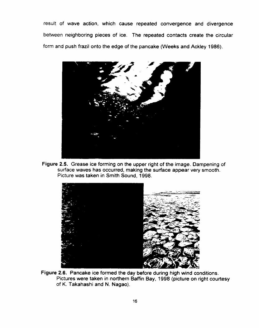
Figure 2.5. Grease ice forming on the upper right of the image. Dampening of surface waves has occurred, making the surface appear very smooth. Picture was taken in Smith Sound, 1998.

Figure 2.6. Pancake ice formed the day before during high wind conditions. Pictures were taken in northern Baffin Bay, 1998 (picture on right courtesy of K. Takahashi and N. Nagao).

The next stage of development is young ice. which has been subdivided into

grey ice (10-15 cm thick) and grey-white ice (15-30 cm thick). This stage

accounts for the transition from new ice and nilas through to first-year ice. New

ice types begin to congeal as they become more compacted and/or a period of

calm and cold conditions occurs (Fig. 2-7). This results in floes or sheets of ice of

varying diameter. Once an ice surface has been produced, sheet ice will begin to

form underneath the congeled grease and/or pancake ice. The ice is now

produced as a result of sensible heat being conducted upward along a

temperature gradient throug h the ice volume. Consequently. ice crystals begin to

grow on the lower surface of the ice sheet as opposed to frazil formation (Weeks

and Ackley 1986). Throughout a thin layer (approximately 5-10 cm), growth

selection is made on crystal orientation. Vertical growth predominates creating a

characteristic ice structure termed columnar or congelation ice (Fig 2.2; Weeks

and Ackley 1986).

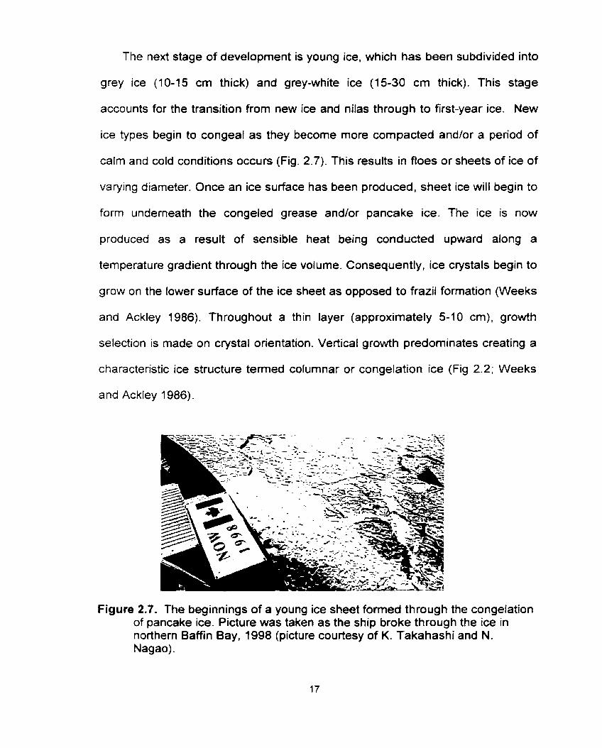
Figure 2.7. The beginnings of a young ice sheet formed through the congelation of pancake ice. Picture was taken as the ship broke through the ice in northern Baffin Bay. 1998 (picture courtesy of K. Takahashi and N. Nagao).

By the end of the young ice stage, sea ice is much less elastic. Finger rafting

no longer occun, although in areas of high wind and ocean stress rafting of

these ice types (Le., one pieœ of ice overriding another) can still occur (personal

observation 1998). More Iikely, ice deformation takes the fom of rubbling

(ridging). For example, pack-ice fioes can have upturned edges similar to

pancake ice, but are the result of floe collisions and subsequent ice edge

deformation. There is also a general trend of lateral ice sheet growth including

the congelation of separate floes. This is due to tighter distributions of floes and

less wave action as a result of the smaller open water area.

The transition from young ice to first-year ice is sirnply a thickness

delineation. First-year ice has also been subdivided into 3 developmental stages

based on its thickness. These stages are temed thin first-year ice (30-70 cm),

medium first-year ice (70-120 cm) and thick first-year ice (> 120 cm). All first-

year ice types are fonned as sheet ice and can be either landfast or pack-ice.

Due to extensive columnar growth, first-year sea ice types have lower

salinities by volume and are much less elastic than the younger ice types (Weeks

and Ackley 1986). As a consequence, rafting becomes much less common.

Under wind and oœan stress, rubbling of first-year ice generally occurs.

Rubbling or ridging occurs due to compressive failures within an ice sheet as

wind and current action cause converging horizontal pressures (Mellor 1986).

This results in the forcing of one portion of the ice sheet upward and the other

downward, foming a sail and keel, respectively. Common results of such ridging

are the formation of extensive linear features temed pressure ridges (Mellor

1986). As mentioned earlier, rubbling can also occur due to collisions between

two separate ice floes. The result is the piling of broken ice above and below

each ice sheet. Extensive rubble fields can form as a result of this type of ice

deformation and are common in areas of high wind andlor current action (Fig.

2.7). During simiiar conditions, first-year ice may also break into smaller floes,

which take angular forms due to linear failures along hydrogen bonds in the ice

(MeIlor 1 986).

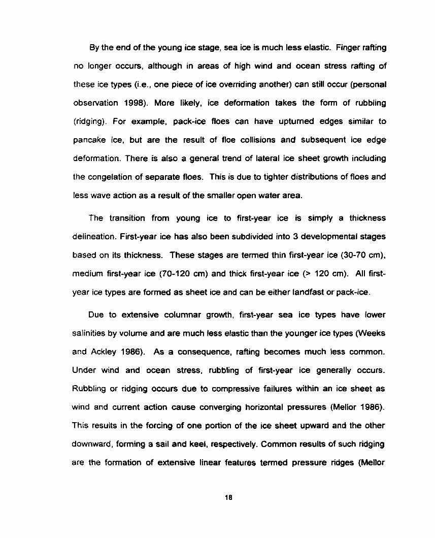
Figure 2.8. Rubble field formed along the southern extent of the North Water polynya of northern Baffin Bay, 1998.

When first-year sea ice remains intact after one melt season, the ice is then

termed old or multiyear ice. The vast majority of the Arctic Basin is covered by

multiyear ice. This ice type is much less saline than first year ice due to

preferential melt of brine pockets and subsequent brine drainage that occurs

during ablation (melt). As a result of brine drainage and melting snow, pockets of

air are formed during freeze-up within the surface layers of rnultiyear ice. This

re-crystallized layer has been termed the active layer (Weeks and Ackley 1986).

The surface of Arctic multiyear ice also demonstrates a characteristic rolling, or

hummocky topography (Fig. 2.9), the result of differential melt and freeze-up due

to snow distribution (Weeks and Ackley 1986). A final feature of multiyear ice is

its floe shape. Floes are generally rounded due to weathering and collisions

between other floes. Further, floe sire can be up to kilometers in diameter.

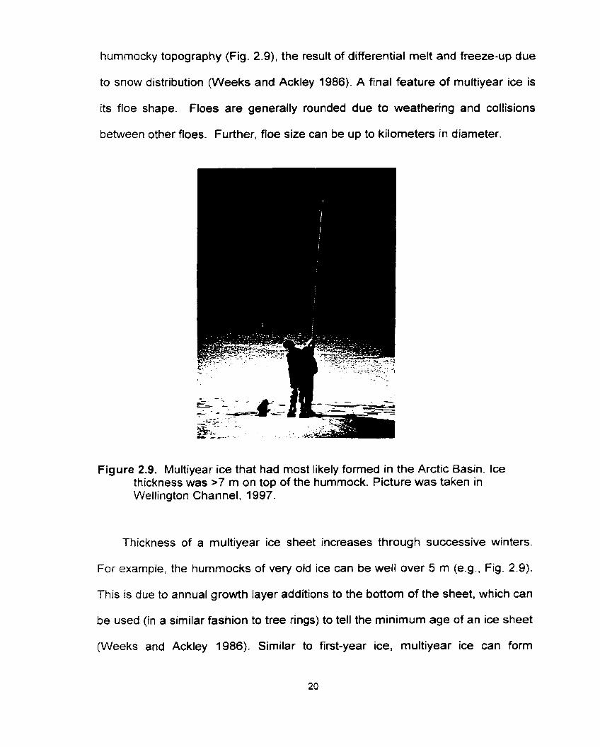
Figure 2.9. Multiyear ice that had most likely formed in the Arctic Basin. Ice thickness was >7 m on top of the hummock. Picture was taken in Wellington Channel, 1997.

Thickness of a multiyear ice sheet increases through successive winters.

For example, the hummocks of very old ice can be well over 5 m (e-g., Fig. 2.9).

This is due to annual growth layer additions to the bottom of the sheet, which can

be used (in a similar fashion to tree rings) to tell the minimum age of an ice sheet

(Weeks and Ackley 1986). Sirnilar to first-year ice, multiyear ice can form

pressure ridges and rubble ice due to wind and current stresses. This

deformation can also act to increase the average thickness of an ice sheet.

2.2 The North Water (NOId(I

In this section I provide a background on the North Water including: an

evolving knowledge on the NOW polynya rnechanisms; records of biological

abundance and the reasons for their high numbers; and the use of remote

sensing in monitoring and investigating the NOW sea ice cover.

2.2.1 The NOW Region

The anomalous region of open water found in northern Bamn Bay has been

documented since the early part of the lïth century. Used by whalers, this region

provided a means to start an early whaling season as a corridor for navigation

into Lancaster Sound (Dunbar 1969; Nutt 1969). The open water was also well

known to peoples of the Thüle culture and later the Danes who founded a trading

seulement in northern Greenland (Dunbar 1969).

Coined as the 'North Water' by the frequenting whalen, the region

encompasses Smith Sound and northern Baffin Bay (Fig. 1.1). The waters are

equally shared between Greenland and Canada. Three recumng polynyas are

recognized wittiin the NOW region: the Smith Sound, Lady Ann Strait and Barrow

Strait - Lancaster Sound polynyas (Steffen 1985). Eventually. the three separate

polynyas become contiguous in the early spring forming the NOW polynya.

2.2.2 Recent History of Knowledge on the NOW Polynya Formation and Maintenance

The formation and maintenance of the North Water polynya has been of

interest since its documented discovery by William Baffin in 1616 (Dunbar and

Dunbar 1972). Many famous explorers frequented the area in an attempt to

decipher how and why the open water occurred. A debate on the physical

mechanisms acting to form and maintain the polynya developed over the

following centuries. Surnmaries of the history of knowledge on the formation and

maintenance of the North Water are available in papers by Nutt (1969) and

Dunbar and Dunbar (1972).

The Smith Sound polynya has drawn most recent attention due to its size,

biological importance and the Iikelihood of a combined latent and sensible heat

mechanism contributing to its formation and maintenance (e-g.. IAPP. 1989;

Smith et al., 1990; Mysak and Huang, 1992; Lewis et al., 1996). Muench (1 971)

had concluded that the main factor behind the polynya's occurrence was the

blockage of ice entering the area due to an ice bridge and the southward removal

of ice due to persistent winds and currents (i.e., a latent heat mechanism). The

scientific community generally accepted this conclusion until Steffen (1985)

documented the occurrence of wann water cells off the coast of Greenland and

other locations within the North Water.

Steffen (1985) concluded through calculations that sensible heat was an

important factor behind the polynya's occurrence throughout winter and early

spring. The possibility of a sensible heat mechanism had long been suspected

(e.g., Nutt 1 969; Dunbar and Dunbar 1 972). The suspected source was a well-

documented warm water layer at depth rnoving northward along the west coast

of Greenland called the West Greenland current. Steffen (1985) was the first to

provide convincing evidence of the current reaching the surface within the NOW.

He suggested the warm water cells' existence could be explained by the coastal

upwelling of relatively wam (> O°C) Batfin Bay Atlantic water from the West

Greenland current. The upwelling being induced through offshore surface water

movement caused in part by the Coriolis force deflecting southward surface

water rnovement to the right. However. Melling et al. (2000) noted that Steffen's

(1985) radiation instruments only measured the ocean's skin temperature,

creating an ambiguous oceanic interpretation of the data.

Bourke and Paquette (1991) were the next to investigate the contribution of

sensible heat in the polynya's formation. Their study focused on the bottom and

deep water of 8affin Bay. They noted the highest temperature between the

surface and a 300 m depth in the vicinity of Smith Sound was -0.6OC. Bourke

and Paquette (1991) concluded that upwelling of this water would not be a

significant factor behind the NOW polynyas occurrence. This would later contrast

with observations by Lewis et al. (1 996).

Modeling efforts followed the work done by Bourke and Paquette (1991).

Mysak and Huang (1992) coupled a latent heat polynya model developed by

Pease (1987) for the NOW polynya with a reduced-gravity, coastal upwelling

model. They concluded that the latent heat mechanism was dominant. However,

Mysak and Huang (1994) did conclude that upwelling, which occurred on a

slower time scale than the latent heat mechanism, played a role in detennining

the polynya width toward the Greenland coast.

Darby et al. (1994) used a nonlinear steady state model with an improved

coastline as a follow up to Mysak and Huang's (1992) efforts. The steady-state

nature of the model limited its application to after the polynya reached an

equilibrium length, or after the polynya had opened. Similar to Mysak and Huang

(1992), Darby et al. (1994) concluded that the latent heat mechanism was

dominant, with the exception of late spring. During late spring, when heat foss to

the atmosphere was reduced, they found the eastern ice edge to be largely

influenced through a sensible heat mechanism.

Lewis et al. (1996) took a new approach to exarnining the possibility of a

contributing sensible heat mechanism. They examined the primary productivity of

the NOW. Collecting biological and oceanographic profiles over a 48 hr period in

mid May, they found temperatures in the West Greenland current to be up to 2.4"

above its freezing temperature ( 1 . 4 O warmer than that observed by Bourke and

Paquette (1991)) and phytoplankton biomass to be greatest along the west coast

of Greenland with a westwarc! decreasing trend. They concluded that sensible

heat can play an important role and substantiated this with observations of higher

primary productivity that occurred along the coast of Greenland relative to the

coast of Canada.

A factor that has not been examined in rnodels or observations of the North

Water is oceanic haline convection caused through brine rejection from freezing

sea ice. Mysak and Huang (1992) noted the possibility, but did not include it in

their model. However, with the high rates of ice production associated with a

latent heat mechanism, one could expect the sensible heat contribution from

haline convection to be substantial.

The debate on the importance of sensible heat contributing to the NOW

polynya has yet to be finafized. Recent manuscripts (2000) by Barber et al.,

Melling et al. and Mundy and Barber continue the debate. These papers are

discussed in Chapters 5 and 6.

2.2.3 Polynyas and Local Biology

The biological importance of recurring polynyas has been noted (Stirling

1980, 1997; Massom 1988). Close correlations have been demonstrated

between recurring polynyas and historic Thüle settlements, whose culture largely

depends on marine rnammals for food (Schledermann 1980). Historically, whaler

obsewations have demonstrated an early spring abundance of rnammals and

seabirds within and near anomalous open water areas in the Arctic pack-ice

(e-g., Nutt 1969). Such observations were indicative of increased biological

productivity (Stirling 1980; 1997). Stirling (1 997) noted the early presence of

whales near polynyas and the observations of whales later in the season

indicated both an early and extended period of food availability. Brown and

Nettleship (1 981) have made similar observations with seabirds demonstrating

that most major colonies of cliff nesting birds in the Canadian Arctic were located

in the vicinity of recurring polynyas. Based on these observations Dunbar (1981)

hypothesized that phytoplankton productivity was high in polynyas. This

hypothesis was later supported (e-g., Hirche et al. 1991 ; Lewis et al- 1996).

The primary explanation for incteased primary production in polynyas, at

least in early spring, is related to light limitation. Solar insolation is the main

limiting factor during the initiation of primary production in sea ice covered waters

(e-g., Gosselin and Legendre 1990; Welch and Bergmann 1989). The

attenuation of photosynthetically active radiation (PAR) through sea ice is

substantial (Maykut and Grenfell 1975). Furthemore, a snow cover can

significantly increase the surface albedo and PAR attenuation (Barry et al. 1993).

With ice concentrations of 90% or less, the effects of snow and ice on PAR

attenuation become negligible due to transmission and reflection of solar

radiation through small leads and cracks. This results in an adequate supply of

diffuse light for primary production to occur (Smith 19â5). In a polynya, these

conditions are available long before adjacent ice covered areas.

Ice algae, a variety of marine microalgae associated with sea ice (also called

sympagic or epontic algae), provide an initial source of primary production as

they are well adapted to the low light levels available beneath the snow and ice

cover. Estimates for ice algal contributions to total primary production range from

10 tu 30% over an annual cycle (Alexander 1974; Welch et al. 1992). Wiihin a

polynya and along its outer edge, the effects of ice and snow on Iimiting ice algal

production would be negligible.

Phytoplankton, primary producers suspended in the water column, account

for the majority of Arctic primary production in an annual cycle (Welch et al.

1992). Both ice and snow cover and water column stability govern light limitation

within the water column. As the water column becomes stratified or the mixed

layer depth (MLD) shallows, phytoplankton can be entrained in an area

favourable to growth relative to light availability (e-g., Maynard and Clark 1987)-

However, once stabilized the water is depleted of nutrients through consumption

and no replenishment. This cycle and 'avoidance' of this cycle has been studied

extensively within the marginal ice zone (ME) and along ice edges where a

phenomenon known as an ice edge bloom occurs (e-g., Alexander and Niebauer

1981 ; Smith and Nelson 1986; Maynard and Clark 1987; Sullivan et al. 1988;

Niebauer and Smith 1989).

Ice edges are very similar to polynyas in that they represent areas of

enhanced biological production with elevated levels of mammals and seabirds

relative to the surrounding ice-covered and ice-free sea. Although the formation

and maintenance of polynyas are much more dynamic than circumstances at a

receding ice edge, the mechanisms acting to enhance biological production are

comparable (Massom 1988). It is also noted that a polynya actually contains an

interior ice edge. Additionally, a polynya's ice edge begins to recede in early

spring, earlier than surrounding ice-covered areas (e.g., Ito 1985).

Maynard and Clark (1987) wmpiled a list of possible components used to

explain ice edge blooms previously proposed in literature. These components

included: water column stratification through input of low-salinity melt water;

nutrient replenishment through wind and tidal driven upwelling at the ice edge; an

inoculum from released ice algal populations; and nutrient replenishment and

distribution control through mesoscale eddies formed along the MIZ. Each

mechanism does not necessarily occur along every ice edge and no single

mechanism is needed for a bloom to occur (Comiso et al. 1993).

Although higher primary productivity has been noted as the most important

factor in explaining elevated mammal and bird abundances within and adjacent

to polynyas (Stirling 1980; 1997; Massom 1988), there are additional

explanations for their high numben. Stirling (1997) nicely summarized these as:

"calmer water, which makes resting on the surface and diving for

food easier than in open sea; access to a substrate to rest upon

after periods in the open water; a temporary banier to migration; a

navigational aid to migrating species; a place where marine

mammals can breathe and seabirds can feed in heavily ice-covered

waters; habitat upon which, or into which. to escape from

predators.. . "

Clearly, explaining the abundance of biology within and adjacent to polynyas

is a complex problem. Further, the explanations used for any particular polynya

will Vary due to different oceanographic and atmospheric conditions. It is clear

though, that the abundance is strongly related to sea ice.

2.2.4 Life within and adjacent to the NOW

In accordance with the previous subsection, the North Water is one of the

most well known biological 'hot spots' in the Arctic. The Thüle culture has had

settlernents in the area for up to 3000 yean. before which it was hypothesized

that the polynya was not present (Schledennann 1980). Whalers used the region

as a means to start an early whaling season (Dunbar 1969; Nutt 1969). Inuit

hunters of Pond Inlet and Arctic Bay of northern Baffin Island also use the area to

hunt narwhals and beluga as they follow leads and cracks away from open water

in early spring (Stirling 1980). These statements alone indicate a consistent

highly productive region with a large marine mammal population to sustain the

human needs.

The NOW is also very important to seabirds. Seabirds forage solely in the

marine environment and therefore need ice free water to gain access to their

prey. Some of the highest seabird concentrations in the world are found within

and adjacent to the region. Every year millions (ca.14 to 30 million pairs) of birds

migrate to the North Water to feed and to breed along both the eastem Canada

and western Greenland coasts, where there are widespread cliffs favourable for

nesting (Nettleship and Evans 1985; Salmonsen 1981 ; Boertman and Mosbech

1998). During shipboard surveys conducted in the North Water, Dovekies (Alle

alle) were the most numerous bird sighted with densities at times of over 1000

birds per square kilometer of water (personal communication N. Kamovsky). The

polynya provides the seabirds with an extended period of time in which they can

conduct their breeding activities, which include: post migration feeding, courtship.

egg laying and incubation, chick rearing, molting and pre-migration feeding

activities. In order to support these numbers of birds, a high level and extended

period of prirnary production would be needed.

Much less information has been collested on the biomass/abundance of

mammals. fishes, plankton and ice algae in the region (IAPP 1989). The NOW

encompasses a vast area and consequently it is hard to estimate numbers frorn

very few observations. Finley and Renaud (1980) found very few marine

mammals during aerial surveys made in mid March and mid May of 1978. They

concluded that the North Water was not a major overwintering area for marine

mammals. This work was re-visited during the International North Water Study

(see section 3.1) by 1. Stirling and M. Holst. They found the NOW to be an

overwintering area for Bbowhead whales (Holst and Stirling 1999) as well as

nanvhals and walruses in accordance with Finley and Renaud (personal

communication M. Holst).

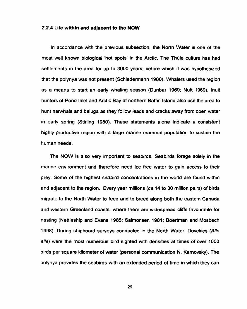
Lewis et al. (1996) observed that chlorophyll a (Chla) concentrations, an

estimate of phytoplankton biomass, was comparable with that of an ice edge

bloom. The highest Chla concentrations occurred along the western Greenland

coast near Northumberland Island with a decreasing trend toward the eastem

Canada coast (Fig. 2.1 0). Chla was also negatively correlated with water column

nutrient concentrations, implying that the bloom had initiated along the Greenland

coast and was progressively moving westward. Phytoplankton was found to

occur in areas where evidence demonstrated the possibility of surface waters

mixing with the West Greenland Current at depth. ft was concluded that there

was a connection between the sensible heat processes occum'ng in the vicinity of

Northumberland Island and the observed phytoplankton bloom (Lewis et al.

1996).

Figure 2.10. Areal concentrations of Chla (mg m-2) in the upper 30 rn (After Lewis et al. 1996).

The International North Water Polynya study (see section 3.1) later based

their hypotheses on Lewis et al.'s (1996) conclusion. Two underlying hypotheses

were proposed: (1) a sensible heat mechanism would be associated with

enhanced primary production due to early stratification, a subsequent warrn

surface rnixed layer and replenishment of nutrients through upwelling; and (2) a

latent heat polynya will be associated with a later primary production bloom due

to late stratification (NOW proposal 1997). It is noted that initiation of primary

production under a latent heat mechanism would still be earlier than adjacent ice

covered areas.

2.2.5 Sea ice in the NOW

The size of the North Water has made it difficult for past explorers to

delineate the extent of open water. Estimates made prior to aircraft and satellite

observations were faulty. For example, the North Water was previously thought

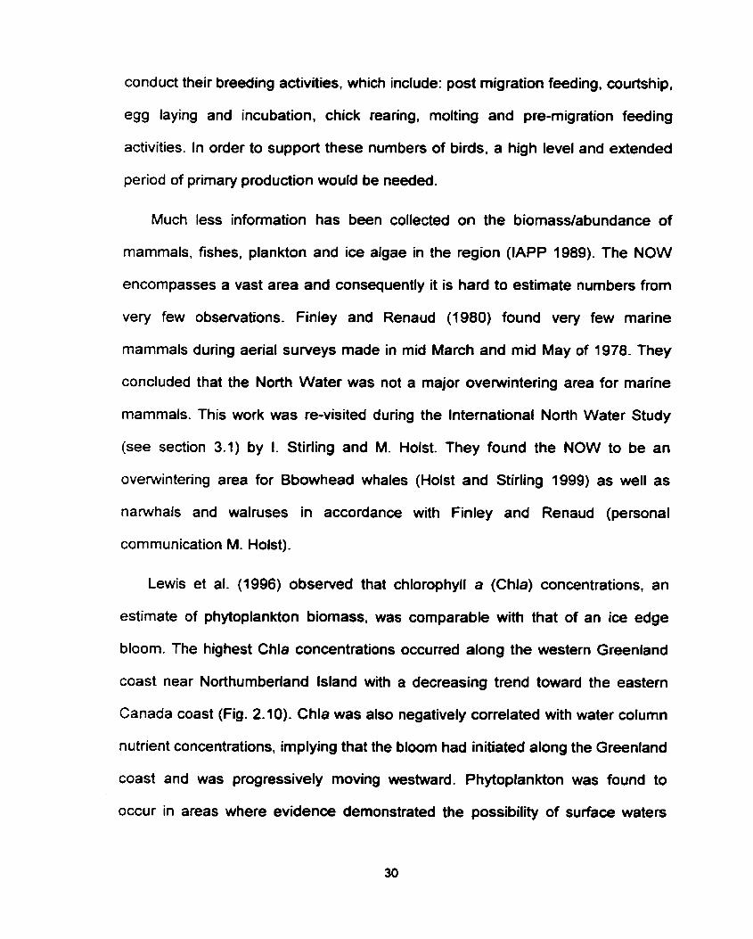
to be open year round (Nutt 1969). Dunbar (1969) was the first to note through

visual aircraft observations that this was not the case. She compiled aircraft

observations made by the US. Naval Oceanographic Office and the Canadian

Meteorological Service between the yean of ?954 to 1968. The data were

averaged showing the first well defined extent of the polynya for the months of

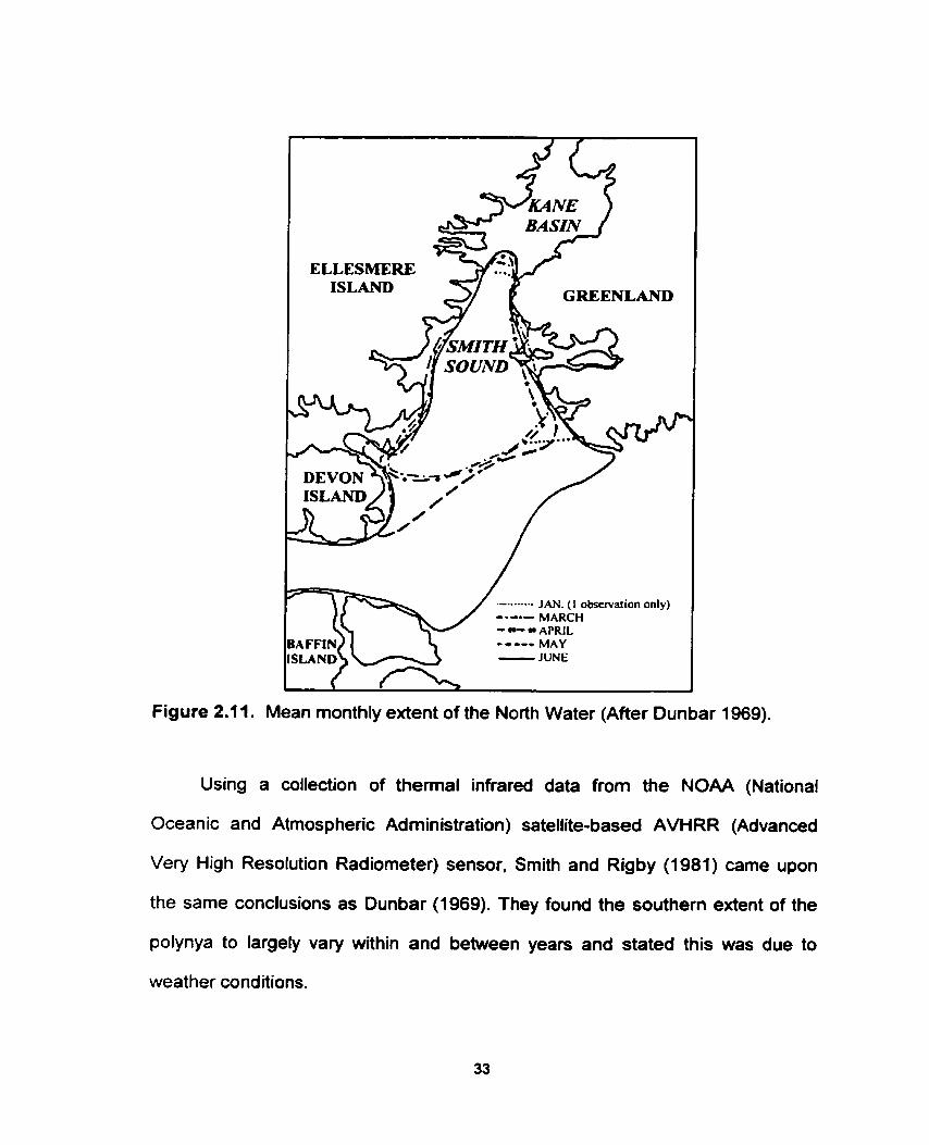
March through June (Fig. 2.1 1). She concluded that the ice edges along the

coasts of Greenland and Canada and within Kane Basin were very consistent

between years. Further, she found the southern ice extent was highly variable

and dependent on climate and season.

In 1971-72, Dunbar (1 972) flew ice reconnaissance flights using radar-scope

photography and visual observations. The results were the first conclusive proof

that the North Water consisted of very little open water during the winter months.

It was found that most open water was restricted to the northem most area near

Smith Sound. She also dernonstrated that small open water patches occurred

throughout the area. creating continual areas of ice formation and many different

types of ice (Dunbar 1972).

.- ..... ... JAN. ( 1 observation only) - - - O - MARCH - - APRIL

FAAND - JUNE

Figure 2.1 1. Mean monthly extent of the North Water (After Dunbar 1969).

Using a collection of thermal infrared data from the NOAA (National

Oceanic and Atmospheric Administration) satellite-based AVHRR (Advanced

Very High Resolution Radiometer) sensor. Smith and Rigby (1981) came upon

the same conclusions as Dunbar (1969). They found the southern extent of the

polynya to largely Vary within and between years and stated this was due to

weather conditions.

Ito and Müller (1982) furthered Smith and Rigby's (1981) statements,

concluding ice motion through Smith Sound was strongly influenced by wind.

They (Ito and Müller) used data from the near infrared channels of the Landsat

sateIlites (1, 2 and 3). By delineating distinct ice features, such as a re-frozen

lead and the edge of an ice floe, and tracking them between images they

determined ice motion. A resultant mean velocity of 4.3 km d-' and speeds up to

34.9 km d-' were observed for ice flowing through Smith Sound (Ito and Müller

1982). These measurements were compared to land-based wind observations,

which demonstrated a strong connection between ice velocity and wind speed.

These were the first large scale measurements of sea ice motion within the

NOW. However, there were large errors associated with their estimations and

satellite data were temporally sparse due to cloud cover.

Sea ice type in the North Water was first examined by Ito (1 985). He visually

classified ice types by grey-tone from the same data set as Ito and Müller (1982).

Subsequently, he was able to distinguish open water, new ice, nilas, grey ice and

'older ice' (grey-white ice and thicker) as well as landfast versus pack-ice. His

observations were made during spring and early summer, as daylight was

needed. Sea ice types and the decay were compared between 2 sub-regions,

one over Smith Sound and one to the south. He found significant variation

between these regions, with higher open water, nilas and grey ice concentrations

within Smith Sound. It was concluded that the North Water consisted of a thin ice

cover in winter and thus ablated earlier than surrounding areas in the spring (Ito

1985). However, no suggestions were made to explain why the North Water

contained thinner ice in early spring.

Steffen (1986) provided the first substantial winter view of the North Watet

sea ice conditions. Through the use of a thermal infrared sensor on board an

aircraft, Steffen (1986) was able to classify six surface classes: open water, dark

nilas, light nilas. grey ice, grey-white ice and white ice (i.e., > 30 cm). Ouring

November, December and January, he found young ice, nifas and open water

covered more than 50% of the Smith Sound polynya. However, the rest of the

region, with the exception of small areas in Lady Ann Strait and Lancaster

Sound, was near 100% white ice cover. Subsequently, Steffen (1986) noted the

polynya in winter was much smaller than previously believed (he quoted Stirling

and Cleator 1981). As well, he noted the open water and young ice were almost

exclusively limited to the coast of Greenland off of Cape Alexander where he had

previously found warm water cells with the same data set (1 985).

During February and March Steffen (1986) found concentrations of white ice

rose to over 50%. It was suggested in passing that extended periods of wind

abatement were responsible for the increasing ice cover. It is noted here and

revisited in Chapter 6 that Steffen's (1986) results tie into Ito's (1985) results,

explaining why thinner ice would occur in the spring.

Agnew (1998) accomplished the next signifiant study on sea ice within or

around the NOW. Although multiyear ice was known to occur within the NOW in

substantial concentrations (e.g., Ito and Müller 1982; de Bastiani 1990), Agnew

(1998) was the first to demonstrate a consistent drainage of multiyear ice from

the Arctic Basin and into the NOW. He did so using animations of 85.5 GHz

SSMll imagery. The drainage was found to periodically stop as ice bridges

formed with Nares Strait and Smith Sound. He also noted the Lincoln Sea. found

at the northern tip of Canada and Greenland (Fig. 1.1). is known to contain some

of the thickest multiyear ice within the Arctic Basin due to deformation as it is

compressed against the northwest coasts of Ellesmere Island and Greenland.

Consequently. the drainage of multiyear ice into the NOW represents a

significant contribution to the freshwater budget that was previously assumed to

be negligible (Aagaard and Camack 1989).

The application of both aircraft- and satellite-based remote sensing to the

study of sea ice cover in the North Water has been dernonstrated. This 'tool'

allows for a much larger spatial and temporal coverage than previously attained

through field measurements. Subsequently, many insights as to how and why

the NOW polynya is formed and maintained were provided. However, there are

still many questions left unanswered. New satellites and sensors, such as

RADARSAT-1 and its onboard Synthetic Aperture Radar (SAR) sensor. are now

better equipped to help answer these questions. Furthemore, there is a trend of

increasing spatial and temporal coverage capabilities of these satellite systems,

which will provide an ever-increasing amount of information.

2.3 Synthetic Aperture Radar

In this section I describe why and how Synthetic Aperture Radar (SAR) is

used extensively as a remote sensing device to detect sea ice types. I further this

discussion with an examination of Grey Level Co-occurrence Matrices (GLCMs)

and their use in aiding sea ice classifications of SAR imagery.

2.3.1 SAR Interactions with Sea Ice

A Synthetic Aperture Radar (SAR) instrument makes use of microwave

energy that is virtually unaffected by al1 weather conditions and can be used day

and night. These facts alone make the use of SAR in polar regions a very

powerful tool. A;: additional advantage of using SAR over polar oceans is a

unique sensitivity to sea ice. This sensitivity has provided the possibility to

distinguish many important surface parameten. Some examples include: open

water, wind velocity, sea ice type, age, concentration and snow cover (e.g.,

Ulaby et al. 1982; Kwok et al. 1992; Bel'chanskiy et al. 1996; Barber and Ngheim

1 998).

SAR is an active rnicrowave system. A SAR instrument transmits microwave

signals or pulses of microwave energy and then records the portion of

transrnitted energy that is backscattered from the observed feature. In a SAR

image, the amount of backscatter is represented with a relative grey-level scale.

For example, the greater the backscatter is, the brighter the image. The amount

of backscatter is dependent on surface roughness. penetration depth of the

transmitted energy and the presence of inhomogeneities within the observed

material (e-g., gas pockets or salinity changes in sea ice) (Ulaby et al. 1982).

These interactions are al1 controlled by the dielectric properties of the observed

material relative to the other materials the signal passes through (e.g., the

atmosphere). Dielectric properties define the electrical conductivity of the

material relative to the wavelength. polarization and incidence angle of the

transmitted energy.

Microwave scattering models separate the scattering process into surface

and volume scattering. The relative complex dielectric constant is computed at

each interface and as an average for each volume. The relative complex

dielectric constant (E*) given in equation 2.1 is used to express the permittivity

(cf) and loss (E") of the material. That is, E' is the ability of electromagnetic energy

to pass into or through a particular interface or volume and E" is a measure of the

transfer of energy to the material. The dielectric constant is expressed as the

complex sum of a real and imaginary part where j is the square root of negative

one.

The extent to which an interface will act as a surface is proportional to the

relative complex dielectric constant (Ulaby et al. 1982).

Discussed earlier, sea ice is a mixture of ice, brine, solid salts (if wld

enough) and gas. Each component possesses a unique dielectric property at

rnicrowave frequencies and can exist in different characteristic sizes. shapes,

volumes and distributions- Dielectric constants for air, ice and brine are

approximateiy 1, 3 and 80, respectively. The proportion of each component

determines the dielectric properties of sea ice. Although small in proportion, the

high dielectric constant of brine significantly influences the dielectric properties of

sea ice.

In a situation where an interface will predominately cause surface scattering

(Le., high relative complex dielectric constant). such as the interface between air

and seawater or saline first-year ice, surface roughness and geometry will

primarily determine the amount of backscatter. Calm open water, grease ice.

nilas and smooth first-year sea ice al1 refiect most of the transmitted radiation

away from the SAR sensor at the same angie as the incidence angle. This type

of reflection is called specular reflection. In a SAR image, these surface types

appear as dark signatures due to small backscatter values. Rougher surfaces,

such as rough open water, rubbled ice and pancake ice, cause a higher

probability of backscatter and therefore appear brighter in a SAR scene. Surface

orientation relative to the sensor can also play a crucial role in the amount of

energy return to the sensor. The degree of surface roughness is actually a

continuum from specular reflection to diffuse reflection where roug hness or

surface variation (h) can be defined by the Rayleigh criterion given in Equation

A h <

8 cos 8

where  and B are the SAR wavelength and incidence angle, respectively (i.e., if

h is true, then the surface is considered smooth).

Like rough surface types, multiyear ice also appears bright in a SAR image.

However, surface scattering is not the dominant scattering type for multiyear sea

ice. In multiyear sea ice most of the brine has drained through preferential melt of

the brine pockets (see section 2.1). The lower salinity results in a lower dielectric

mismatch at the air-ice interface. This allows a greater penetration of the radar

signal into the ice volume, which then interacts with interna1 inhomogeneites of

the ice. The result is volume scattering.

Volume scattering is dependent on the density, size and geometric shape of

scatterers. Scatterers have to be large enough to be resolved or 'seen' by a

particular frequency in order to affect the signal. That is, the radar will interact

with these ice inclusions only if their characteristic dimensions are at least one

tenth that of the radar wavelength (Ulaby et al. 1982). Further, as the size of the

particies approaches the wavelength of the signal, scattering increases. The re-

crystallized active layer in rnultiyear ice primarily detemines the amount of

backscatter. The air pockets within this layer (Fig. 2.2) can cause, if large

enough, significant scattering making the ice type appear bright in a SAR image.

As described above, SAR scattering over sea ice is largely dependent on the

ice type. Backscatter over fint-year sea ice with a saline surface is primarîly

dependent on surface roughness with very little volume scattering. Alternatively,

the low salinity of a multiyear ice active layer and the presence of substantial

volume scatters result in a greater importance of volume scattering to the SAR

return. These unique interactions cause varying returns between different sea ice

types, allowing for the possibility of their discrimination within a SAR scene.

However, the distinction between various ice types is not perfect based purely on

backscatter. Additional methods such as using spatial information (e-g., texture

and contextual information) have to be employed to further distinguish ice types.

2.3.2 The Grey level Cooccurrence Matrix

Many investigations attempting to classify Synthetic Aperture Radar (SAR)

data have explored the use of spatial information in an attempt to automate or

assist in delineating different sea ice types (e-g., Homes et al. 1984; Barber and

LeDrew 1991 ; Nystuen and Garcia 1992; Barber et al. 1993; Smith et al. 1995;

Soh and Tsatsoulis 7999). The majority of these approaches examined second-

order texture statistics derived from Grey Level Co-occurrence Matrices (GLCM).

Haralick et al. (1973) first defined the use of a GLCM in classifying imagery.

The GLCM represents one of many second-order statistical approaches to

texture analysis. For clarification, a first-order approach uses image tone (i.e., the

grey level values representing relative backscatter in a radar image). Examples

of first-order statistics in radar imager- include the mean, standard deviation and

range of a window of pixels (e.g., Nystuen and Garcia 1992). Second-order

statistics also make use of grey level. The fundamental difference is that a

second-order approach provides a measure of the spatial information between a

pixel (image resolution ceIl) and its neighbors (Barber et al. 1993). The use of

second-order approaches such as a GLCM derived statistic also adds

robustness to the discrimination of SAR sea ice classes. Further, Shokr (1991)

found evidence that secondorder texture measures provide unique values for ice

types, independent of absolute image calibration, a common problem with SAR

imagery.

The GLCM provides the conditional joint probabilities of al1 pixel pairwise

combinations within a given computational window sire. Many different

aigorithms are available to extract specific information from the GLCM. Each

provides a separate measure of localized texture. Therefore, some statistics

outperform others in delineating sea ice types.

Holmes et al. (1984) accomplished one of the earlier studies on the use of

texture analysis on SAR imagery. They confinned the usefulness of applying a

GLCM approach to delineate ice floe boundaries and discriminate multiyear from

first-year ice types. Studies by Barber and LeDrew (1991) and Shokr (1991)

demonstrated the power of different texture statististics individually and in

combinations. However, not al1 classification studies have shown the same

success in the use of GLCM statistics. For example, Nystuen and Garcia (1992)

demonstrated only a marginally improved classification through the use of GLCM

statistics and rewmmended that first-order statistics should be used in order to

minimize computational effort. Smith et al. (1995) supported these results though

it was apparent that calibration of the SAR images had to be accomplished prior

to the use of grey level and fint-order texture statistics.

There appears to be a trade-off between the absolute calibration of images

and the use of second-order texture statistics. Noted above, second-order

textures can provide unique values for ice types independent of absolute

calibrations (Shokr 1991). Barber et al. (1993) also noted that a second-order

approach would be more dependent on the relative spatial variation. Therefore,

second-order texture measures can provide unique information on the spatial

variation of grey tones.

In this chapter I have reviewed al1 major aspects pertaining to my thesis. In

the first section I described the evolution of sea ice types in differing

environments and subsequent characteristics including some key definitions that

will be used throughout this thesis. In the second section I described the North

Water and provided a recent history of knowledge on the NOW polynya

rnechanisms, documents of biological abundance and the potential reasons for

their high numbers and the use of remote sensing in monitoring and investigating

the NOW sea ice cover. A description of SAR interaction with sea ice was

included in the final section. This also included a bnef description of the use of

GLCMs in SAR sea ice classifications. In the next chapter I describe the methods

used in this thesis. This includes descriptions of the data collection, Geographic

Information System (GIS) framework and data analysis.

CHAPTER 3: METHODS

In this chapter I describe the data used in this thesis and how it was analyzed

to meet my stated objectives. The chapter is presented in four interrelated

sections: (1) the lnternational NOW Polynya Study, the project from which data

were collected for this thesis; (2) the data sets used here, including both satellite

and field data and the methods employed to collect and validate the data; (3) the

Geographic Information System (GIS) framework that was designed and

implemented for the purpose of this thesis; and (4) the spatial and temporal

analytical methods used to meet my thesis objectives.

3.7: The International North Water Polynya Study

In 1990, the Arctic Ocean Science Board launched the lnternational Arctic

Polynya Programme (IAPP) initiative with the following mission statement: '10

intençively study the physical/meteorological processes leading to the formation

of polynyas and of the biological and biogeochemical processes taking place

within their boundaries" (IAPP 1989).

The North Water polynya is considered to be one of the most productive

areas above the Arctic Circle and is located at a latitude thought to be impacted

early and significantly by the present trend in climate change (NOW Proposal

1997). As a result, many leading Arctic specialists from Canada and abroad

(Denmark, Poland, United States, Japan, Mexico, Belgium and the United

Kingdom) proposed the highly integrative and multidisciplinary International North

Water Polynya Study. This was the second polynya study (the fint was the

Northeast Water Polynya Study in the Greenland Sea during 1992 and 1993) to

be initiated under the umbrella of the IAPP. The NOW project was built around a

central hypothesis linking biological productivity of the North Water to local

climatic and oceanographic forcing (see Chapter 2) while exploring the response

of the ecosystem to the climate change scenario through modeling (NOW

Proposal 1997). During the summer of 1997 (onboard the CCGS Louis SE

Laurent) and the spring and summer of 1998 (onboard the CCGS Piem

Radisson) field data of various oceanographic, meteorological, biological and

biog eochemical variables were successfully collected within the NOW polyn ya.

Data used in this thesis were collected during the 1998 expedition.

3.2 Data

Critical for understanding the mechanisms behind polynya formation and

maintenance is our ability to monitor thern. During The International North Water

Polynya Study (NOW study) 1998 expedition both satellite and field data were

collected. In this section I describe these data, including the methods used to

collect and validate them.

3.2.1 RADARSAT-1 Data

Launched in 1995, RADARSAT-1 is the newest satellite-borne SAR sensor

providing unequalled spatial and temporal coverage of the polar seas. A total of

153 ScanSAR Wide A and B beam mode images were obtained from

RADARSAT-1 over the period January 21 through December 7, 1998 (Canadian

Ice Service (CS)). RADARSAT-1 has an operating frequency of 5.3 GHz with

HH polarization. ScanSAR images were acquired over the NOW with the

following characteristics: swath width of 460 km; 100 rn pixel spacing; 8 bit pixels;

and swath lengths variable from 1000 to 2000 km. Incidence angles ranged

between 20° and 49O across a single scene. Temporal gaps between images

ranged from 12 hours to 1 week. The data were also uncalibrated with

characteristics such as inter-beam seams and unbalanced radiometric levels

across an image causing image intensity to be brighter in the near range.

Images were attained as blocks or segments in a ScanSAR file format, which

were processed at the Central Data Processing Facility (CDPF) in Gatineau,

Quebec. Each segment was 5000 lines long, with the exception of the final block

that was variable in length. Typical scenes were 2 to 4 segments long (i.e., 1000

to 2000 km). Image blocks were concatenated into one scene before use.

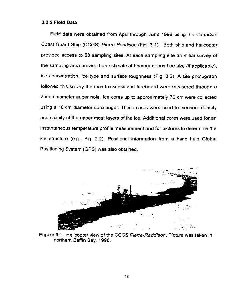
3.2.2 Field Data

Field data were obtained from April through June 1998 using the Canadian

Coast Guard Ship (CCGS) Pierre-Raddison (Fig. 3.1). Both ship and helicopter

provided access to 68 sampling sites. At each sampling site an initiai survey of

the sampling area provided an estimate of hornogeneous floe size (if applicable).

ice concentration. ice type and surface roughness (Fig. 3.2). A site photograph

followed this survey then ice thickness and freeboard were rneasured through a

2-inch diameter auger hole. Ice cores up to approximately 70 cm were collected

using a 10 cm diameter core auger. These cores were used to measure density

and salinity of the upper most layers of the ice. Additional cores were used for an

instantaneous temperature profile measurement and for pictures to determine the

ice structure (e-g., Fig. 2.2). Positional information from a hand held Global

Positioning System (GPS) was also obtained.

Figure 3.1. fielicopter view of the CCGS Pierre-Raddison. Picture was taken in northern Baffin Bay, 1998.

Figure 3.2. Pictures of starting a sample site after being craned to the sea ice sample site via a metal 'basket' (a) and sampling an ice floe approximately 50 m in diameter (b). The CCGS Pierre-Raddison is visible in the background of the picture b. Pictures were taken in northern Baffin Bay, 1998 (Pictures courtesy of K. Takahashi, N. Nagao and E. Key).

For inaccessible sites (e-g.. thin ice or small floe sue) a Hi8 video camera

was used to document ice type, concentration and floe size. Near continuous

video was obtained from a camera mounted on the bridge of the CCGS Pie-

Radisson with periodic visual observations of sea ice conditions input to a

database. Input to the database included a time stamp and a geographic position

obtained from a GPS mounted on the roof of the bridge. Daily check-ups were

used to confirm the computer clock was at the same time as the camera clock.

A camera was also mounted on a helicopter and systematic grid surveys

were flown in the vicinity of the ship. Flight times were planned near satellite

overpass times. They were flown at an opportunistic basis dependent on

weather, location and helicopter allocation time. Flight plans followed a 25 km x

25 km square grid pattern that was separated into 5 transects, each 25 km long

with a north-south orientation. Before a flight, both the carnera and computer

docks were synced with the helicopter's GPS clock. As the camera was mounted

on the rear of the helicopter (Fig. 3.3). the camera was turned on prior to the

flight. During a flight the computer was plugged directly into the helicopter's GPS

and logged the helicopter's position in real time. The passenger in the front of the

helicopter also manually logged the fiight. This included recordings of: the start

and stop time of each transect; the helicopter's altitude and speed at the

beginning and end of each transect; identified ice types and the time of the

observations; and percent cloud cover.

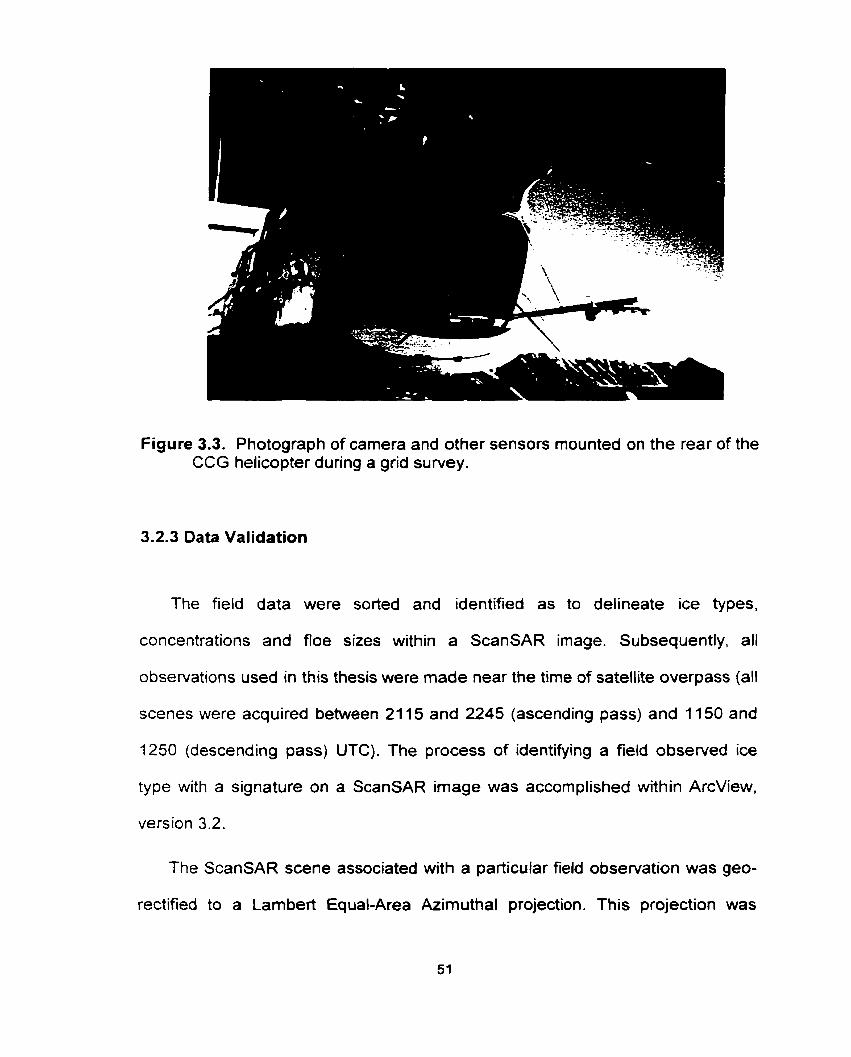
Figure 3.3. Photograph of camera and other sensors rnounted on the rear of the CCG helicopter during a grid survey.

3.2.3 Data Validation

The field data were sorted and identified as to delineate ice types,

concentrations and floe sizes within a ScanSAR image. Subsequently. al1

observations used in this thesis were made near the time of satellite overpass (al1

scenes were acquired between 21 15 and 2245 (ascending pass) and 11 50 and

1250 (descending pass) UTC). The process of identifying a field observed ice

type with a signature on a ScanSAR image was accomplished within ArcView,

version 3.2.

The ScanSAR scene associated with a particular field observation was geo-

rectified to a Lambert Equal-Area Azimuthal projection. This projection was

chosen as to rninimize the amount of image distortion from the geo-rectification

process (also termed image warping andlor geocoding). In order to geo-rectify a

ScanSAR image, Ground Control Points (GCPs) were used. GCPs were

associated with each image line within a processed ScanSAR file. The latitude

and longitude of the first, middle and last column of each image line were

extracted from the file using a program called ScanSAR Viewer (developed by

CIS). A Macro was written in Excel to extract 100 equally spaced sets of first,

middle and last column positions into a new spreadsheet. This spreadsheet of

300 positions was used to geo-rectify an image.

The GCPs were plotted over both the ScanSAR image and projection using

the ArcView extension "Image Warp". A third order polynomial was chosen for

the warping forrnulae. This resulted in a Root Mean Squared (RMS) error

between 1 and 2 pixel units for each image. RMS error is an estimation of how

well the GCPs fit from the image ont0 the projection as a result of the warping

formulae. Consequently. the RMS error implied that each GCP for an image was

warped within 100 to 200 m of the projected GCP. Although this error was larger

than the pixel size, it was accepted for the purpose of locating validation

signatures of ice types.

The field data were first sorted as being dec ted close to the tirne of an

acquired ScanSAR scene. The latitudes and longitudes associated with the field

data were plotted ont0 the same EqualArea projection and matched to

signatures on each ScanSAR scene. Validating the field observation location was

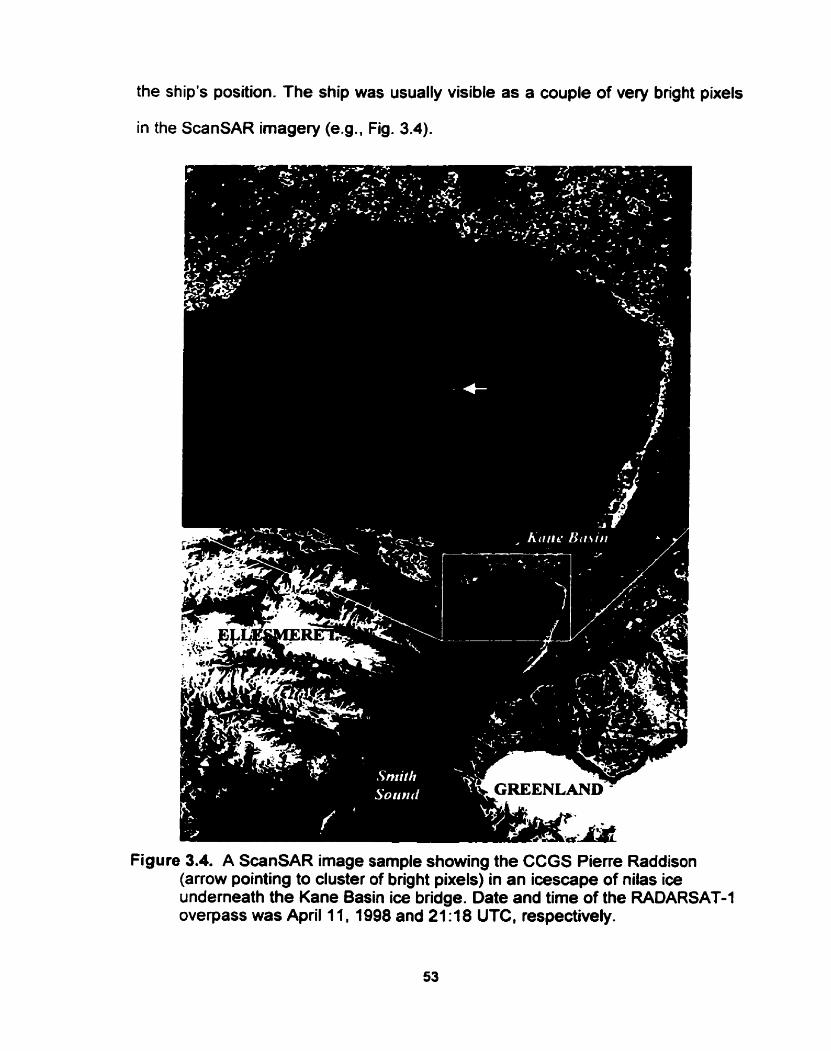
the ship's position. The ship was usually visible as a couple of very bright pix

in the ScanSAR imagery (e.g.. Fig. 3.4).

Figure 3.4. A ScanSAR image sample showing the CCGS Pierre Raddison (arrow pointing to cluster of bright pixels) in an icescape of nilas ice underneath the Kane Basin ice bridge. Date and time of the RADARSAT overpass was April 1 1, 1998 and 21 : 18 UTC, respectively.

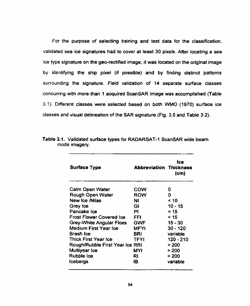
For the purpose of selecting training and test data for the classification.

validated sea ice signatures had to cover at least 30 pixels. After locating a sea

ice type signature on the geo-rectified image. it was located on the original image

by identifying the ship pixel (if possible) and by finding distinct patterns

surrounding the signature. Field validation of 14 separate surface classes

concurring with more than 1 acquired ScanSAR image was accomplished (Table

3.1). Different classes were selected based on both WMO (1 970) surface ice

classes and visual delineation of the SAR signature (Fig. 3.5 and Table 3.2).

Table 3.1. Validated surface types for RADARSAT-1 ScanSAR wide beam mode imagery.

Surface Type Ice

Abbreviation Thickness (cm)

Cairn Open Water COW Rough Open Water ROW New Ice /Nilas NI Grey Ice GI Pancake Ice PI Frost Flower Covered Ice FFI Grey-White Angular Floes GWF Medium First Year Ice MFYI Brash lce BR1 Thick First Year lce TFY l Rough/Rubble First Year Ice RRI Multiyear Ice MY1 Rubble Ice RI lce bergs IB

O O < 10 10- 15 < 15 < 15 15 - 30 30 - 120 variable 120 - 210 > 200 > 200 > 200 variable

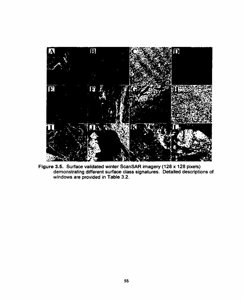
Figure 3.5. Surface validated winter ScanSAR imagery (128 x 128 pixels) demonstrating different surface class signatures. Detailed descriptions of windows are provided in Table 3.2.

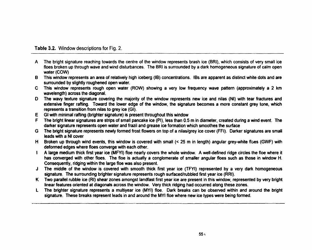
Table 3.2. Window descriptions for Fig. 2.

The bright signature reaching towards the centre of the window represents brash ice (BRI), which consists of very small ice floes broken up through wave and wind disturbances. The BRI is surrounded by a dark homogeneous signature of calm open water (COW) This window represents an area of relatively high iceberg (16) concentrations. 10s are apparent as distinct white dots and are sumunded by slightly roughened open water. This window represents rough open water (ROW) showing a very low frequency wave pattern (appraximately a 2 km wavelength) across the diagonal. The wavy texture signature cavering the majority of the window represents new ice and nilas (NI) with tear fractures and extensive finger rafting. Toward the lower edge of the window, the signature becomes a more constant grey tone, which represents a transition from nilas to grey ice (GI). GI with minimal rafting (brighter signature) is present throughout this window The bright linear signatures are strips of small pancake ice (PI), less than 0.5 m in diameter, created dudng a wind event. The darker signature represents open water and frazil and grease ice formation which smoothes the surface The bright signature represents newly formed frost flowers on top of a nilaslgrey ice cover (FFI), Darker signatures are small leads with a NI cover Broken up through wind events, this window is covered with small (< 25 m in length) angular grey-white f l m (GWF) with deformed edges where floes converge with each other. A large mdium thick first year ice (MFYI) floe nearly coven the whole window. A well-defined ridge circles the floe where it has converged with other floes. The fioe is actually a conglomerate of smaller angular floes such as those in window H. Consequently, ridging within the large floe was also present. The middle of the window is covered with smooth thick first year ice (TFYI) represented by a very dark homogeneous signature. The sunounding brighter signature represents rough surfacedlrubbled first year ice (RRI). Two parallel rubble ice (RI) shear zones amongst landfast first year ice are present in this window, represented by very bright linear features oriented at diagonals across the window. Very thick ridging had occurred along these zones. The brighter signature represents a multiyear ice (MYI) floe. Dark breaks can be observed within and around the bright signature. These breaks represent leads in and around the MY1 fioe where new ice types were k i n g formed.

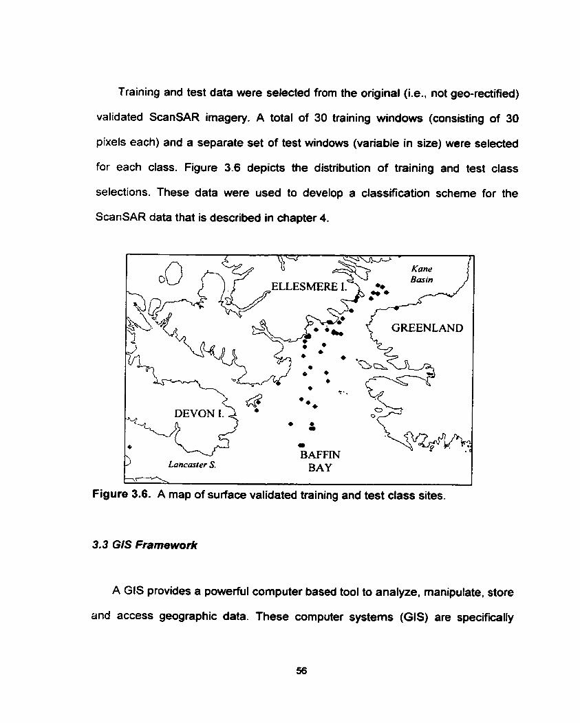
Training and test data were selected from the original (Le., not geo-rectified)

validated ScanSAR imagery. A total of 30 training windows (consisting of 30

pixels each) and a separate set of test windows (variable in size) were selected

for each class. Figure 3.6 depicts the distribution of training and test class

selections. These data were used to develop a classification scheme for the

ScanSAR data that is described in chapter 4.

Lancaster S. tL

O 0 9

9

% 0

BAFFIN BAY

GREENLAND C

--

Figure 3.6. A map of surface validated training and test class sites.

3.3 GIS Framework

A GIS provides a powerful computer based tool to analyze, manipulate, store

and access geographic data. These computer systems (GIS) are specifically

designed to discard redundant data and to organize data. making it easily

accessible to the user. This is accomplished through the organization of data into

databases or 'layers' that may be linked spatially or though a unique identifier.

Additional information, temed attribute data, may be added to the databases.

This section describes the GIS framework used in this thesis.

Satellite-borne remote sensing in the form of Synthetic Aperture Radar (SAR)

provided the core data set for this study. fnherent W h such a data set is a large

data volume. For example. one satellite data scene was approximately 60

rnegabytes of digital data. Consequently. both satellite coverage and data

volume issues helped to delineate the study region (Fig. 3.7).

Version 3.2 of Arcview, a Geographic Information System (GIS) software

package, was employed in the analysis. The GIS was used to discard redundant

data and organize data into a framework for analysis (Fig. 3.7). The base of the

GIS framework consisted of a 2 x 2 km vector based grid system. The grid

consisted of 90.868 cells centered over the NOW in a Lambert Equal-Area

Azmuthal projection with a central meridian of 55"W and reference latitude of

90°N (Fig. 3.7). Each cell was assigned a unique identifier, which provided links

between databases (Fig. 3.7). Data used to populate the GIS databases were

percent cover of each surface type extracted following classification of the

ScanSAR imagery (see chapter 4).

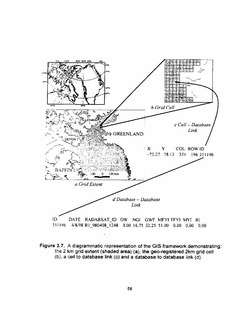
a Grid Exrenl

d Darabase - Darabase Link

ID DATE MDARSAT-ID OW NGI GWF MFYI TFYI MY1 RI 35 I 196 1/8i198 RI - 980408-1 248 0.00 16.75 32.25 5 1 .O0 0.00 0.00 0.00

Figure 3.7. A diagrammatic r2presentation of the GIS framework demonstrating: the 2 km grid extent (shaded area) (a), the geo-registered 2km grid cell (b), a cell to database link (c) and a database to database link (d).

3.4 Analytical Design

To meet the second and third objectives of this thesis, the analysis first

examined the sea ice spatio-temporal patterns. The objectives followed that by

observing these patterns I would highlight the nature of the physical processes

that create and maintain the polynya. The polynya mechanisms would also be

related to biological production as explained previously. In this section I describe

the analyses used to meet the second and third objectives of this thesis.

The analysis to meet the second objective was split into a spatial and

temporal approach. The first approach defined the database temporally and

examined the spatial structure of ice cover, whereas the second approach

defined the database spatially and examined the temporal evolution of ice cover.

The first approach focused on three temporal periods: (1) prior to the Kane

Basin ice bridge formation, (2) after the Kane Basin ice bridge formation and

before melt onset and (3) after fall freeze-up, hereafter referred to as winter.

spring and fall, respectively. The spring and fall periods were delineated as

before melt onset and after freezing conditions, respectively, with no defined

summer period due to the absence of an ice type classification throughout this

time. A buffer of at least five days between commencement and completion of

periods was used. Consequently. the periods included data from January 21

through February 28 (10 scenes). March 17 through May 26 (40 scenes) and

October 15 through December 7 (32 scenes) for winter, spring and fall.

respectively.

The grid data were averaged into the three periods and statistical analysis

was used to examine the spatial patterns of sea ice typekoncentration for each

period separately. The structure of ice cover was exarnined through a k-means

convergence cluster analysis on al1 surface types for each period. This was

accomplished within the statistical software package SPSS, version 8.0. The k-

means procedure takes a nonhierarchical approach, providing an econornical

method for cluster analysis on large data sets. This method is accomplished by

assigning each data unit (grid cell) to the nearest initial k cluster centroid (based

on an Euclidean rnetric) (Anderberg 1973). New centroids for each gaining

cluster are recomputed and data units reassigned to the nearest centroid. The

final result is obtained through an iterative process, repeated until a user defined

convergence between the previous and resultant centroids is reached. A 1

percent convergence was used for this analysis. For each period, 2 through 6

clusters were examined iteratively based on the cluster centroid values for each

surface type. Selection of the optimal k clusten was defined as that point where

no new information was obtained when examining k + 1.

Additionally, the mean surface type concentration along a 50 km transect

was calculated for comparison with similar observations made by Steffen (1 986).

The 50 km transect was located just west of Cape Alexander (Fig. 3.8).

The second approach examined the temporal evolution of sea ice cover in

defined sub-regions. lnterpretation of the first approach results prompted the

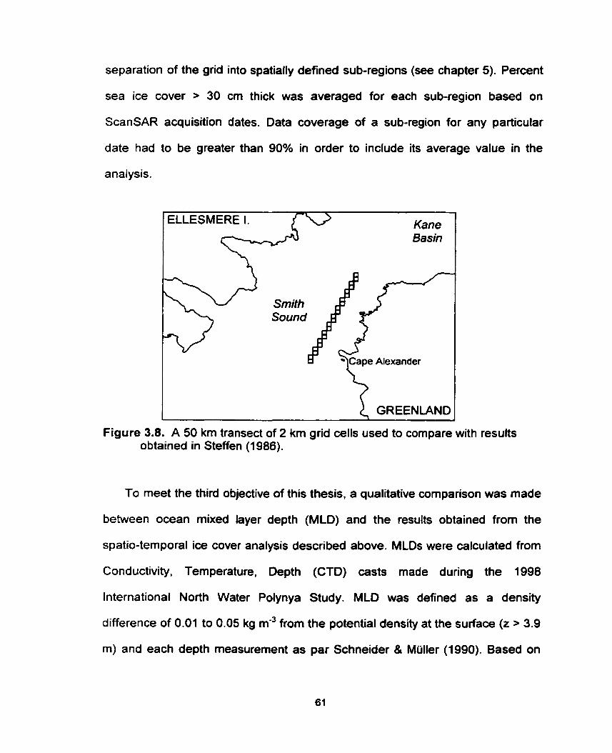
separation of the grid into spatially defined sub-regions (see chapter 5). Percent

sea ice cover + 30 cm thick was averaged for each sub-region based on

ScanSAR acquisition dates. Data coverage of a sub-region for any particular

date had to be greater than 90% in order to include its average value in the

analysis.

ELLESMERE 1.

Basin

GREENLAND

Figure 3.8. A 50 km transect of 2 km grid cells used to compare with results obtained in Steffen (1 986).

To meet the third objective of this thesis, a qualitative cornparison was made

between ocean mixed layer depth (MLD) and the results obtained from the

spatio-temporal ice cover analysis described above. MLDs were calculated from

Conductivity, Temperature, Depth (CTD) casts made during the 1998

International North Water Polynya Study. MLD was defined as a density

difference of 0.01 to 0.05 kg m" from the potential density at the surface (z > 3.9

rn) and each depth measurement as par Schneider 8 Müller (1990). Based on

each Leg of the 1998 NOW study expedition, these data were interpolated to a

grid using the inverse distance weighted method provided in Arcview, version

3.2. A 10 km radius surrounding each CTD cast point observation was used as a

fixed distance for interpolation.

This chapter was written to describe the data used and the methods

employed to meet rny thesis objectives. In the first section I described the

lnternational North Water Polynya Study, from which data for this thesis were

collected. Following this was a description of both the RADARSAT-1 ScanSAR

wide beam mode imagery and field data collected during the 1998 expedition of

the lnternational NOW study. Further, I described the methods used for data

collection and data validation. A brief description of the Geographic Information

System used to organize data into a framework for analysis was presented. In

the final section I described the analytical methods used in the thesis. The next

chapter was included out of necessity, as no sea ice classification scheme

applicable to this study had been developed for ScanSAR imagery.

Subsequently, in chapter 4, 1 discuss a ScanSAR classification scheme that was

developed for the purpose of this thesis.

CHAPTER 4: SCANSAR SEA ICE CLASSIFICATION OF THE NORTH WATER

The classification of SAR data into sea ice types is a necessity for many

polar science projects. For example, a detailed study of ocean-sea ice-

atmosphere interactions, such as the International North Water Polynya study,

requires the classification of as many different ice types as possible.

Unfortunately, the development of an automated classification scheme or

algorithm has not yet been successfully accomplished. The developrnent has

been Iirnited by absolute calibration problems of the SAR data and the fact that

different ice types may have over-lapping tonal values (e.g., Barber et al. 1991;

Kwok et al. 1992; Smith et al. 1995). Classification algorithrns have been

developed for operational use (Wohl 1995; Ramsay et al. 1997; Shokr et al.

1999). However. none have been fully automated in that they are al1 dependent

on visual interpretations of the imagery from experienced interpreters. Additional

methods for improving the classification of SAR include the use of texture (e.g.,

Barber et al. 1993) and information fusion using data from different satellite

sensors (e-g., Haverkamp and Tsatsoulis 1999). These methods have at least

begun to reduce some of the ambiguities associated wlh SAR data.

In this thesis. RADARSAT-1 ScanSAR wide beam mode images were used.

There was no available or suitable (for the purpose of this thesis) classification

algorithm developed for use with uncalibrated ScanSAR data. Therefore, a new

classification scheme was developed and implemented for the purpose of this

thesis. The scheme was not fully automated in that it used both tonal and textural

information contained within the ScanSAR imagery and visual interpretation of

the irnagery. Furthenore, the sire of the data set created the necessity for an

efficient approach that maximized classification precision and minimized image-

processing time.

In this chapter I describe the purpose built ScanSAR classification scheme. I

split the chapter into 3 sections that describe: (1) the texture statistics that were

used as distinguishing variables in the classification scherne; (2) the methods

used to develop the classification scherne; and (3) the resultant hierarchical

classification scheme used in this thesis.

4.1 Texture Statisfics

Studies have demonstrated that when used by itself. image tone in a SAR

scene is not able to discriminate between different sea ice types and open water

with similar grey levels (e-g., Barber et al. 1991 ; Kwok et al. 1992; Smith et al.

1995). To alleviate this problem, the implementation of spatial information was

introduced to assist in classification of sea ice types in SAR imagery (e-g.,

Holmes et al. 1984). There is a large number of different approaches available to

obtain spatial information from a SAR scene including both first-order (e-g.,

Nystuen and Garcia 1992; Smith et al. 1995) and second-order approaches (e-g.,

Barber and LeDrew 1991). The use of a Grey Level Occurrence Matrix (GLCM)

is only one of these approaches. However, studies such as Barber et al. (1993)

have dernonstrated that texture measures calculated from a GLCM outperfarm

other approaches.

GLCMs provide the conditional joint probabilities of al1 pixel pairwise

combinations within a given computational window size (Barber et al. 1993). That

is, a GLCM is specified by the relative frequency of grey level co-occurrences

made by grey level i with grey level j, which are separated by a given

displacement vector and confined to a given computational window. The

displacement vector is specified by the conditional parameten. interpixel

sampling distance (6) and orientation (a). Following Haralick et al. (1973), the

computation of a GLCM can be expressed algebraically as Equation 4.1, where

Cg is defined in Equation 4.2. For example:

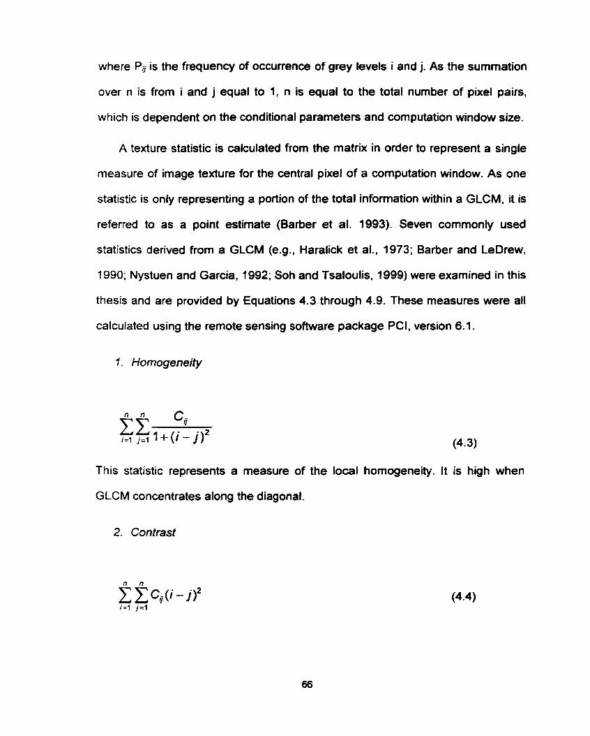
where Pu is the frequency of occurrence of grey levels i and j. As the summation

over n is from i and j equal to 1, n is equal to the total number of pixel pairs,

which is dependent on the conditional parameters and computation window size.

A texture statistic is calculated from the matrix in order to represent a single

measure of image texture for the central pixel of a computation window. As one

statistic is only representing a portion of the total information within a GLCM, it is

referred to as a point estimate (Barber et al. 1993). Seven commonly used

statistics derived from a GLCM (e-g., Haralick et al., 1973; Barber and LeDrew,

1990; Nystuen and Garcia, 1992; Soh and Tsaloulis, 1999) were examined in this

thesis and are provided by Equations 4.3 through 4.9. These measures were al1

calculated using the remote sensing software package PCI, version 6.1.

1. Homogeneity

This statistic represents a measure of the local homogeneity. It is high when

GLCM concentrates along the diagonal.

2. Contrast

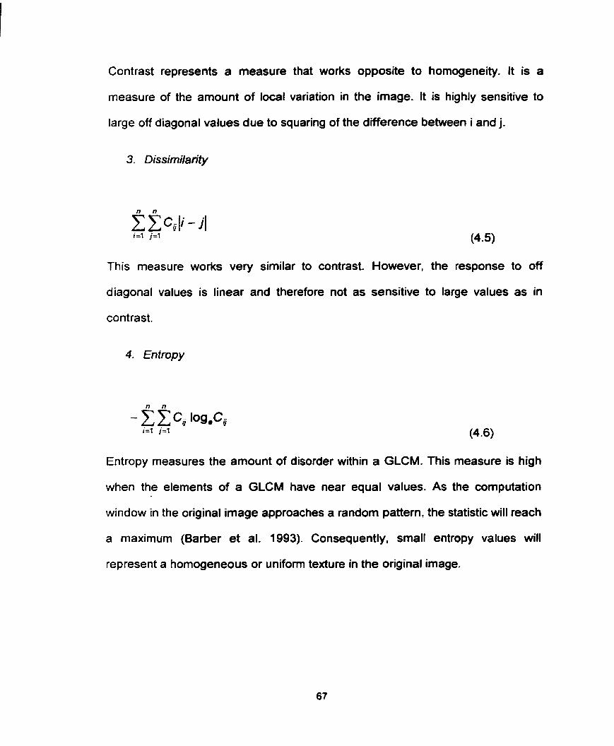
Contrast represents a measure that works opposite to homogeneity. It is a

rneasure of the amount of local variation in the image. It is highly sensitive to

large off diagonal values due to squaring of the difference between i and j.

This measure works very similar to contrast. However, the response to off

diagonal values is Iinear and therefore not as sensitive to large values as in

contrast.

4. En tropy

Entropy measures the amount of disorder within a GLCM. This rneasure is high

when the elements of a GLCM have near equal values. As the computation

window in the original image approaches a random pattern. the statistic will reach

a maximum (Barber et al. 1993). Consequently, small entropy values will

represent a homogeneous or uniforrn texture in the original image.

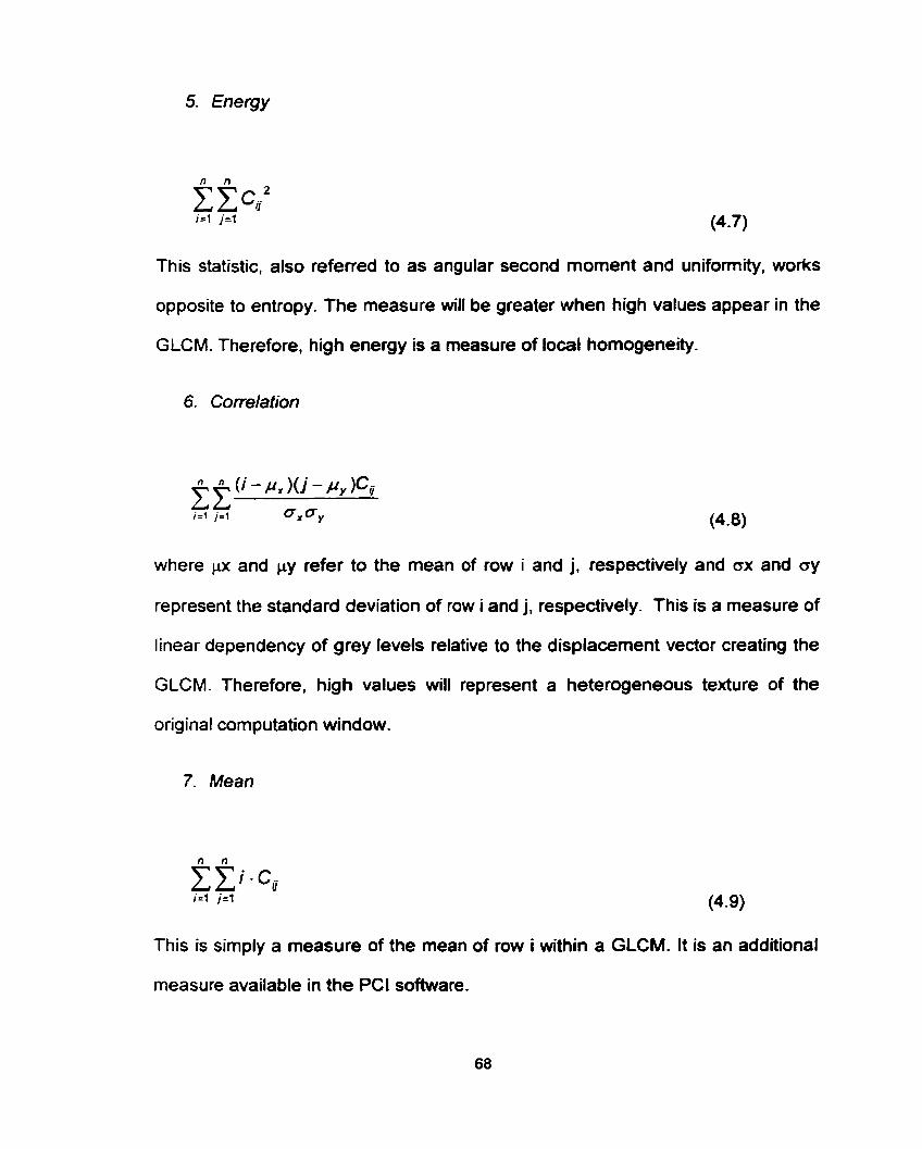
This statistic, also referred to as angular second moment and uniformity, works

opposite to entropy. The measure will be greater when high values appear in the

GLCM. Therefore, high energy is a measure of local homogeneity.

6. Correlation

where px and py refer to the

(4.8)

mean of row i and j, respectively and ox and ay

represent the standard deviation of row i and j, respectively. This is a measure of

linear dependency of grey levels relative to the displacement vector creating the

GLCM. Therefore, high values will represent a heterogeneous texture of the

original computation window.

This is simply a measure of the mean of row i within a GLCM. It is an additional

measure available in the PCI software.

Before the above texture statistics were calculated, the conditional

parameters, quantization scheme and computational window size had to be

decided upon. Barber and LeDrew (1991) have demonstrated when examining

the surface texture of SAR sea ice types, the GLCM conditional parameters, 6

and a gave optimum results when equal to 1 and O" (parallel to SAR look

direction), respectively. Consequently, these parameters were used in this thesis.

Furthermore, prior to the formation of a GLCM, data were quantized (in this case

from 256 to 16 grey levels) in order to keep the time for matrix computations

moderate. Soh and Tsatsoulis (1999) have shown 8 level quantization to be

unrepresentative of an original 256 level data set, whereas a 64 level

representation provided optimal results. However, time required to process 64

levels was deemed to be excessive in this case due to the extrernely large data

volume of SAR imagery. A decision was made to quantize to 16 levels and

justified based on results of Marceau et al. (1990). A 7 by 7 pixel window was

also chosen for GLCM computations. This window was large enough to calculate

a rneaningful joint-distribution of grey tones, yet small enough to delineate a

surface type (Shokr et al. 1995).

4.2 Classification Procedure

Using SPSS, version 8.0, a Multiple Oiscriminate Analysis (MDA) was

performed on the training data. A MDA works in a similar fashion to a Principal

Component Analysis (PCA), however it maximires inter-group variation as

opposed to maximizing variation over the complete data matrix (Manly 1986).

Based on N dimensions (Le., distinguishing variables), a MDA calculates N-1

canonical discriminate functions that maximize the discrimination between k a-

priori groups in a diminishing order. That is, the first canonical discriminate

function maximizes the inter-class variation by minimizing the residuals. The

second function also maximizes the inter-class variation, however is Iimited to

being statistically orthogonal to the previous function, and so on (Manly 1986). In

this thesis, N was initially represented by 8 variables; grey level and 7 texture

statistics, whereas k was initially represented by 14 surface classes (Fig. 3.5 and

Tables 3.1 and 3.2). A contingency table that demonstrates the training data

performance on distinguishing itself using a Mahalanobis minimum distance

classifier is outputted by the MDA in SPSS. The resultant contingency table was

examined and logical decisions were made to discard or pool classes. A MDA

was then performed on the new set of classes. An iterative merge and split

classification process was repeated until the criterion of an overall agreement of

90% or greater was obtained amongst the training data.

The pooled within-gmups absolute correlation between a discriminating

variable and standardized canonical discriminate functions was used to

determine the best discriminates. These variables were further examined using

the Maximum Likelihood Classification (MLC) technique available as part of the

Multispectral Package in PCI. A MLC uses the training data means and standard

deviations to calculate normally distributed probability density functions that are

used to determine if a pixel falls within a class or not. Following the MLC, a 7 by

7 mode filter was used to smooth out erroneously c!assified outlier pixels. The

resuits were compared with the independent set of test windows. In order to

eliminate chance agreement behnreen the classified and test pixels, the Kappa

coefficient (K) and standard deviation (Ks) were used to represent the overall

classification agreement (Bishop et al. 1975).

Once the MLC and filter pass were employed, areas of open water, new

pack-ice, old pack-ice and Iandfast ice were visually identified and a polygon was

used to segment these areas. lnterpretation of the four surface categories largely

followed Volume II of the operational Canadian Ice Service SAR Ice

Interpretation Guide (1 994). Additional information was obtained through

examination of the images in a temporal sequence. For example, landfast ice

was defined as ice that had not moved for a penod of 3 days.

Three images were randomly selected to examine reproducibility of the

manual digitization procedure. An open water polygon was outlined on each.

Areas for each polygon were extracted. The polygons were deleted and then re-

digitized with the area of each polygon extracted. This procedure was repeated

10 times. Each area calculation was divided by the maximum observed area for

each separate polygon, normalizing the observations to 1. The resultant 30

samples were used to calculate a standard deviation as an estimation of error.

Once classified into surface ice type, images were geo-rectified to the grid's

projection using the 300 GCP spreadsheet obtained from each ScanSAR file

(see section 3.2.3). Percent cover of each surface type was then extracted into

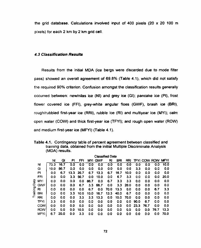
the grid database. Calculations involved input of 400 pixels (20 x 20 100 m

pixels) for each 2 km by 2 km grid ceIl.

4.3 Classification Results

Results from the initial MDA (ice bergs were discarded due to mode filter

pass) showed an overall agreement of 69.8% (Table 4.1). which did not satisfy

the required 90% criterion. Confusion amongst the classification results generally

occurred between: newlnilas ice (NI) and grey ice (GI); pancake ice (PI), frost

Rower covered ice (FFI), grey-white angular floes (GWF), brash ice (BRI),

roughlrubbled first-year ice (RRI). rubble ice (RI) and muitiyear ice (MYI); calm

open water (COW) and thick first-year ice (TFYI); and rough open water (ROW)

and medium first-year ice (MFYI) (Table 4.1).

Table 4.1. Contingency table of percent agreement between classified and training data, obtained frorn the initial Multiple Discriminate Analysis (MDA) results.

C bssified Data

NI GI PI FFI

2 MY1 5 GWF .E RI .g BR1

RRI TFY 1 cow ROW MW1

FFI MYIGWF RI BR1 0.0 0.0 0.0 0.0 0.0

Rf3i TFYI COW ROW MFYI 0.0 0.0 0.0 0.0 10.0

The decisions employed to improve the overall agreement included: (1) the

rernoval of PI, BRI, FFI, ROW and RRI; and (2) pooling of NI and GI. and COW

and TFYI. PI, BR1 and FFI ice were removed due to low intemal agreements of

13.3%, 43.0% and 57.0%, r~spectively, following the previous decision results.

NI and GI were pooled as they were very similar ice classes with low class

separation. This resulted in a new combined surface class, newlnilas-grey ice

(NGI). COW and TFYI were pooled due to low signature distinction. However,

they were later distinguished in the digitization decision rule step (see below).

ROW had a relatively low separation and was removed for later distinction using

the digitized masks. RRI was discarded because the range of its distinguishing

variables substantially overlapped with those of GWF and RI types. This had

caused GWF and RI types to have lower interna1 agreements. The removal and

pooling of the various classes mentioned above resulted in an overall agreement

that increased to 92.9%.

The final MDA results were used to choose the best discriminating variables.

The GLCM mean statistic and grey level showed the highest correlation with the

first canonical discriminate function (Table 4.2). Entropy and homogeneity texture

statistics demonstrated the highest correlation with the second canonical

discriminate function (Table 4.2). Furthemore, the fint two orthogonal axes

accounted for ove? 95% of the cumulative variation. Consequently, these 4

variables were found to be the best discriminators and were further compared

using the MLC results.

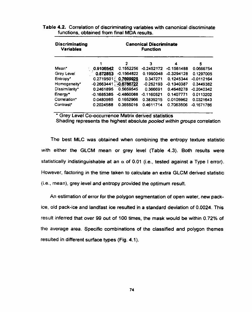
Table 4.2. Correlation of discriminating variables with canonical discriminate functions, obtained from final MDA results.

Discrirninating Variables

Canonical Discriminate Function

1 2 Mean* . - O.Qlû6542 0.1552256 Grey Level - - 0.872853 -0.1 564822 Entropy' 0.27 1 950 1 0,76-!@@!@ Homogeneity' -0. 2663441 L32676661 Dissimilarity' 0.2461 895 0.5659545 Energy 4.1685385 4.4860088 Correlation' 0.0480985 O. 1652966 Contraste 0.2024588 0.3655016

* Grey Level Co-occurrence Matrix derived statistics Shading represents the highest absolute pooled within groups correlation

The best MLC was obtained when combining the entropy texture statistic

with either the GLCM mean or grey level (Table 4.3). Both results were

statistically indistinguishable at an a of 0.01 (i.e., tested against a Type I error).

However, factoring in the time taken to calculate an extra GLCM derived statistic

(Le., mean), grey level and entropy provided the optimum result.

An estimation of error for the polygon segmentation of open water, new pack-

ice, old pack-ice and landfast ice resulted in a standard deviation of 0.0024. This

result inferred that over 99 out of 100 times, the mask would be within 0.72% of

the average area. Specific combinations of the classified and polygon themes

resulted in different surface types (Fig. 4.1).

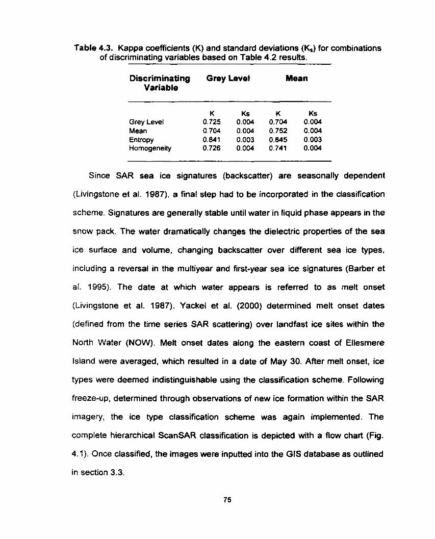
Table 4.3. Kappa coefficients (K) and standard deviations (KI) for combinations of discrirninating variables based on Table 4.2 results.

Discriminating Grey Level Mean Variable

K Ks K Ks Grey Level 0.725 0.004 0.704 0.004 Mean 0.704 0.004 0.752 0.004 Entropy 0.841 0.003 0.845 0.003 Homogeneity 0.726 0.004 0.741 0.004

Since SAR sea ice signatures (backscatter) are seasonally dependent

(Livingstone et al. 1987). a final step had to be incorporated in the classification

scheme. Signatures are generally stable until water in liquid phase appears in the

snow pack. The water dramatically changes the dielectric properties of the sea

ice surface and volume, changing backscatter over different sea ice types,

including a reversal in the multiyear and first-year sea ice signatures (Barber et

al. 1995). The date at which water appean is referred to as malt onset

(Livingstone et al. 1987). Yackel et al. (2000) detennined melt onset dates

(defined from the time series SAR scattering) over landfast ice sites within the

North Water (NOW). Melt onset dates along the eastern coast of Ellesmere

Island were averaged, which resulted in a date of May 30. After melt onset, ice

types were deemed indistinguishable using the classification scheme. Following

freeze-up, deterrnined through observations of new ice formation within the SAR

imagery, the ice type classification scheme was again implemented. The

complete hierarchical ScanSAR classification is depicted with a flow chart (Fig.

4.1). Once classified, the images were inputted into the GIS database as outlined

in section 3.3.

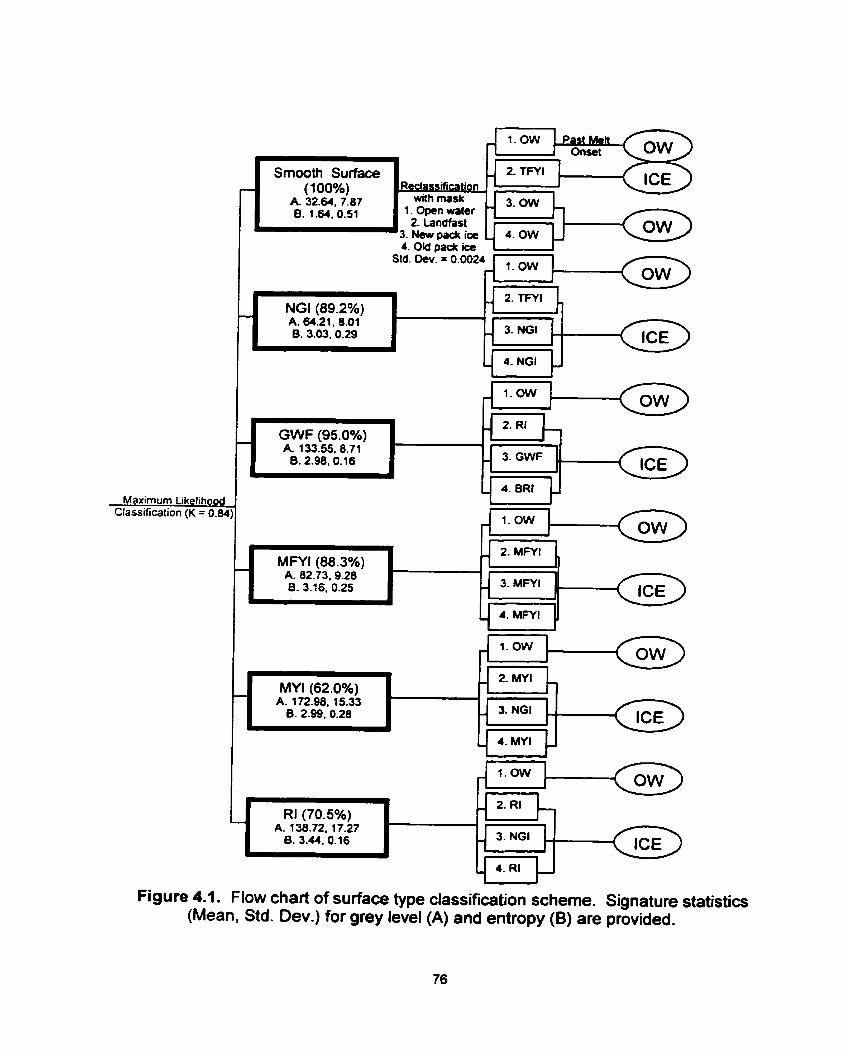
- 1.0W ,

- 2. RI - GWF (95.0%) - A. 133.55. 8.71

B. 2.98. 0.16 - 3.GWF I -

-&&&4t - 1.OW

Figure 4.1. Flow chart of surface type classification scheme. Signature statistics (Mean, Std. Dev.) for grey level (A) and entropy (6) are provided.

2.MFYI

- 3.MFYI

- 4. MFYI ,

-

--

- 1.OW

MFYI (88.3%) A. 82-73.9.28 6-3-16, 0.25

Std. Dev. = 0.0024 ' OW

L

NGI (89-2%) 'i1

A. 64.21. 8.01

I B. 3.03.0.29

- ,

- Onset

2 . m 1

-

4. Old pack iœ

3-0W

4. ow

- -

MY1 (62.0%) A. 172.98. 15.33

B. 2.99. 0.28

'3. ~cwpack iœ

L

Smooth Surface (100%)

A. 32.64. 7.87 6. 1.64, 0.51

- -

Rectwification with mark

1-openMer 2. Landfast

2.MYI

3. NGI

4. MY1

- ,

-

After the images were classified, an additional error source was observed in

the data. The classification scheme resulted in the delineation of an extensive

area as having near 100% young ice cover off the Coast Greenland near Cape

York. This result was improbable and attributed to the location of the original

training data collection. Training and test data collection occurred toward the

northwest side of the NOW (Fig. 3.4). This is an area of constant disturbance,

with high current and wind velocities. In an area such as this, the only smooth

surfaced pack-ice types are new ice types formed during calm conditions with

minimal rafting (e-g., the original NI and GI training data). After such a break in

the 'normal' conditions, ocean or atmospheric disturbances would cause the ice

to raft and deform, in essence, roughening the surface. This would cause an

increase in SAR backscatter. Consequently, as the classification moves further

from the location of training data site locations, delineation is more of smooth

versus rougher ice types as opposed to newer versus older ice types,

respectively. Considering the volume of ice, a relative delineation can be made in

that smoother ice is relatively thinner than rougher ice that has been compacted

and deformed.

In this chapter I described the development of a purpose built hierarchical

classification scheme to classify sea ice types within RADARSAT-1 images. This

included: (1) a description of how the distinguishing variables were obtained from

the ScanSAR imagery, (2) a description of the methods used to develop the

classification scheme and (3) the classification results and finalized scheme. In

the next chapter I present the results and discussion of the analysis used to meet

objectives 2 and 3 of this thesis.

CHAPTER 5: RESULTS AND DISCUSSION

In this chapter I examine the spatial and temporal patterns of the North Water

(NOW) sea ice cover using the data and analysis described in the two previous

chapters. I relate the obsewed patterns to the physical polynya mechanisms and

biological implications in the NOW polynya by examining three interrelated

themes: (1) sea ice spatial patterns; (2) sea ice temporal evolution and (3)

relationships between the mixed layer depth and sea ice patterns.

5.1 Sea /ce Spatial Patterns

The k-means cluster approach provided a natural grouping of ice typeiopen

water concentration combinations, demonstrating a clear structural pattern within

each seasonal period. This statistical distinction provided the basis for inferences

from natural ice type combinations to the physical mechanisms that could cause

the cornbinations. The main trends were obsewed when k equaled 3 or 4

clusters, depending on the period being analyzed. As more clusters were

specified for a k-means analysis, no additional spatial structure was observed.

5.1.1 Winter Period

Spatial structure of the region for the winter period (WP) was best

represented with 4 clusters (Fig. 5.1). WP cluster 1 consisted mainly of high

TFYl concentrations and was located within the landfast ice along al1 coasts.

Thick first-year ice (TFYI) was an extensive stationary surface class restricted to

sheltered landfast ice. which explained the grouping of landfast TFYI with itself.

WP cluster 2 represented a combination of medium RI and MN1

concentrations and the highest MY1 concentrations relative to other cluster

compositions (Fig. 5.1 ). Throug hout Smith Sound and south, grid cells classified

as cluster 2 were found toward the west side of the region. following the eastem

coast of Canada. Predominate composition of this group consisted of rough

surface classes inferring an area of high ocean andfor wind stress. This result is

consistent with the well-documented southward currents and predorninate

norîherly winds along this area (e-g., Nutt 1969; Muench and Sadler 1973;

Barber et al. 2000).

Cluster 2 also populated nearly 100% of the grid celis just north of Smith

Sound (Fig. 5.1). This clumped distribution had classified an area of high MY1

and RI concentrations (Fig. 5.2a and b, respectively). This observation can be

explained by: (1) Kane Basin at this location narrows considerably, which would

cause the congestion of sea ice; (2) the composition of large MY1 floes could act

to block the northern entrance to Smith Sound; and (3) cold temperatures would

cause further congelation of separate ice fioes.

Cluster/ Percent Cover (%)

O W 0.25 0.77 0.76 2.05 NGI ! .O4 9.33 23.80 78.54 GWF 0.01 0.70 2.1 1 0.13 MFYI 10.18 38.88 58.60 17.95 TFYI 86.15 1.94 2.22 0.20 MY1 0.68 13.31 2.00 0.20

Figure 5.1. 1998 winter period (Jan. 21 through Feb. 28) k-means cluster results for the GIS grid. The table provides the mean surface type composition for each blue-shaded cluster.

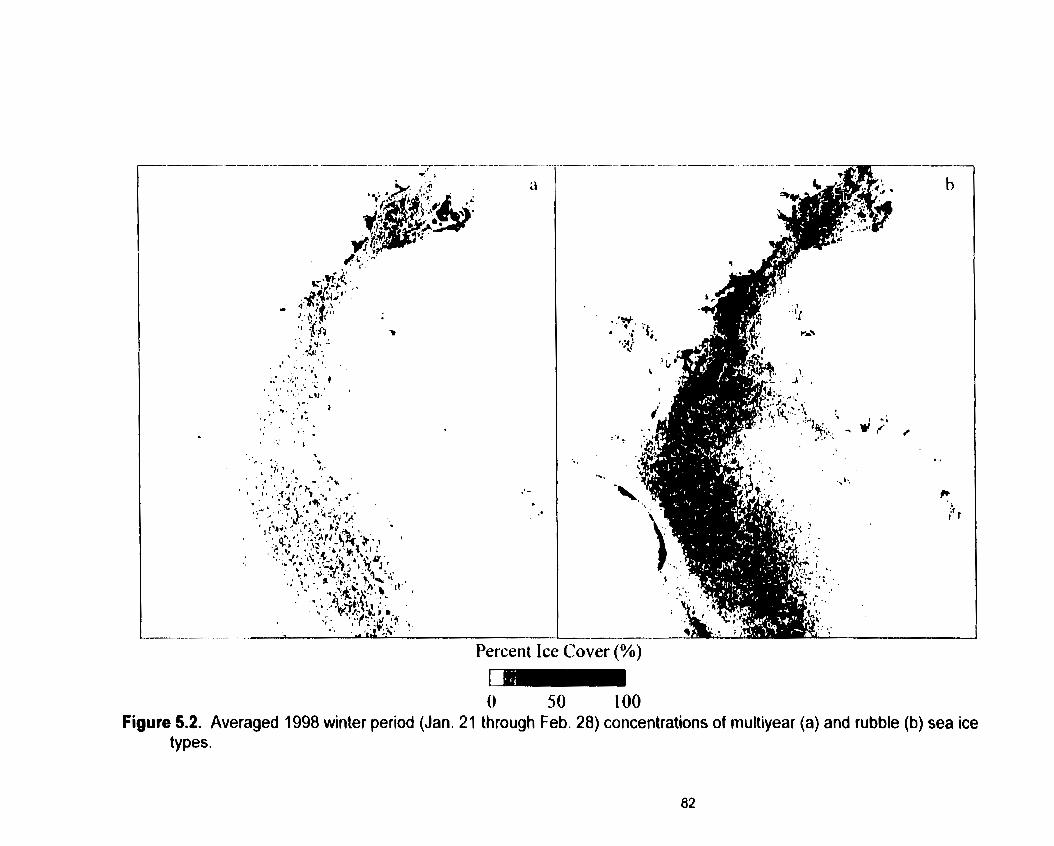
Percent Ice Cover (%)

- - -

Figure 5.2. Averaged 1998 ~ i n t e r period (Jan. 21 through Feb. 28) concentrations of inultiyear (a) and rubble (b) sea ice types.

Multiyear ice has been observed through animations of 85.5 GHz SSM/I

(Special Sensor Microwave Imager) to penodically drain through Nares Strait

alternating with the formation of ice bridges along its path towards Baffin Bay

(Agnew 1998). Therefore, the majority of MY1 found in this area would have an

Arctic Basin origin. Furthemore, the Lincoln Sea. found at the northern tip of

Canada and Greenland (Fig. 1.1). is known to contain some of the thickest MY1

within the Arctic Basin due to deformation as it is cornpressed against the

northwest coast of Greenland.

With no Kane Basin ice bridge present during the winter period, cluster 2

may also be interpreted as depicting a uthoroughfaren of sea ice. Ito and Müller

(1 982) had calculated a mean ice velocity of 4.3 km-d-' in a southward direction

through Smith Sound with a maximum observation of 34.9 km-d-', which was

strongly influenced by wind. Further, Wilson et al. (2000) found monthly averaged

ice velocities of up to 8.64 km-d-' (March, 1998) through Smith Sound. These

southward sea ice velocities combined with thick MY1 composition represent a

poorly documented contribution to the freshwater flux out of the Arctic Basin into

Baffin Bay.

The tendency of cluster 2 to occur tightly along the western side of the region

through and south of Smith Sound may be interrelated with the distribution of

cluster 3 (Fig. 5.1). Composition of cluster 3 for the winter period was a

combination of NGI and MFYl with relatively high GWF concentrations. Steffen

(1985) documented a consistent occurrence of warrn water celfs off the wast of

Greenland near Cape Alexander and Cape York. He explained the cells'

existence as the upwelling of wann (O°C) Atlantic Baffin Bay water compensating

a mass movement of water westward throughout Smith Sound. With congestion

of sea ice in Kane Basin and the presence of strong and consistent northerly

winds, the Coriolis force deflects surface mass flow to the right of the wind,

inducing upwelling along the Greenland coast (Steffen 1985). The spatial

distributions and compositions of WP clusters 2 and 3 throughout Smith Sound

support this explanation. These distributions within Smith Sound c m be

additionally explained through katabatic (downslope) winds off the coast of

Greenland. Bromwich et al. (1996) have modeled strong downslope winds over

the Greenland Ice Sheet driven mainly by radiative cooling of the sloping terrain.

Their results, substantiated through surface observations, demonstrated strong

(> 10 m S-') offshore winds. which deviate to the right (north) due to the Coriolis

force. In the vicinity of Smith Sound. these katabatic winds would be opposite in

direction to the predominate northerly winds documented for the area. Therefore.

these winds could cause divergence of ice off the coast of Greenland. Similar to

Steffen's (1985) explanation. offshore mass transport of surface waters could

cause upwelling of warm Atlantic waters from depth. There is no way of

distinguishing between an oceanic and atmospheric forcing on this ice using the

NOW study 1998 data set. Thus this observation is left as a speculation

consistent with the same general observations of Steffen (1 985).

Cluster 4 grouped the lowest concentrations of RI and MYI. Therefore. the

spatial transition from clusters 2 through 3 to 4 infers a trend of decreasing ice

deformation towards Greenland and west into Lancaster Sound. This obsewation

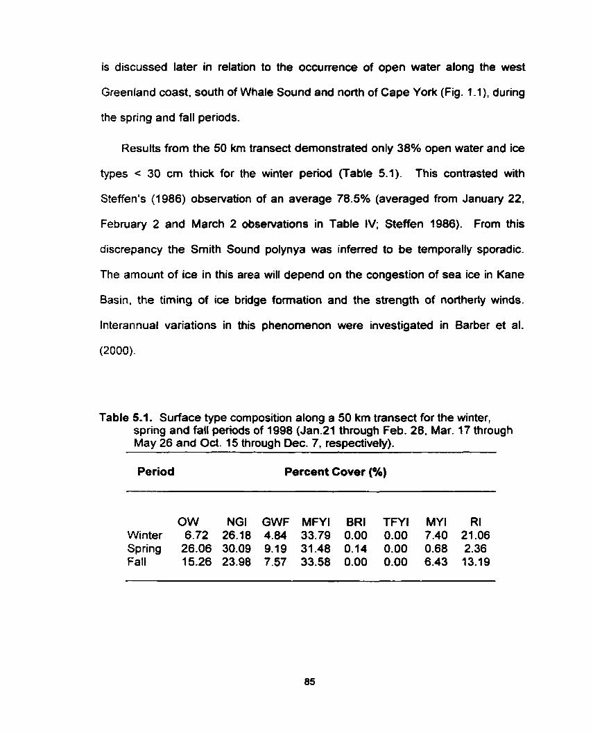
is discussed later in relation to the occurrence of open water along the west

Greenland coast, south of Whale Sound and north of Cape York (Fig. 1 A), during

the spring and fall periods.

Results from the 50 km transect demonstrated only 38% open water and ice

types c 30 cm thick for the winter period (Table 5.1). This contrasted with

Steffen's (1986) observation of an average 78.5% (averaged from January 22,

February 2 and March 2 observations in Table IV; Steffen 1986). From this

discrepancy the Smith Sound polynya was inferred to be temporally sporadic.

The amount of ice in this area will depend on the congestion of sea ice in Kane

Basin, the timing of ice bridge formation and the strength of northerly winds.

lnterannual variations in this phenornenon were investigated in Barber et al.

(2000).

Table 5.1. Surface type composition along a 50 km transect for the winter, spring and fall periods of 1998 (Jan.21 through Feb. 28, Mar. 17 through May 26 and Oct. 15 through Dec. 7 , respectively). -

Period Percent Cover (%)

OW NGI GWF MFYI BR1 TFYl MY1 RI Winter 6.72 26.18 4.84 33.79 0.00 0.00 7.40 21.06 Spring 26.06 30.09 9.19 31.48 0.14 0.00 0.68 2.36 Fall 15.26 23.98 7.57 33.58 0.00 0.00 6.43 13.19

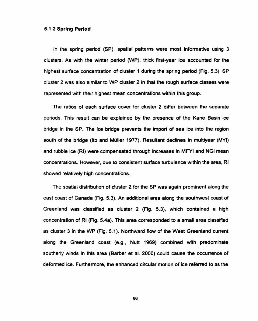
5.1.2 Spring Period

In the spring period (SP), spatial patterns were most informative using 3

clusters. As with the winter period (WP), thick first-year ice accaunted for the

highest surface concentration of cluster 1 during the spring period (Fig. 5.3). SP

cluster 2 was also similar to WP cluster 2 in that the rough surface classes were

represented with their highest mean concentrations within this group.

The ratios of each surface cover for cluster 2 differ between the separate

periods. This result can be explained by the presence of the Kane Basin ice

bridge in the SP. The ice bridge prevents the import of sea ice into the region

south of the bridge (Ito and Müller 1977). Resultant declines in multiyear (MYI)

and rubble ice (RI) were compensated through increases in MFYl and NGI mean

concentrations. However, due to consistent surface turbulence within the area, RI

showed relatively high concentrations.

The spatial distribution of cluster 2 for the SP was again prominent along the

east coast of Canada (Fig. 5.3). An additional area along the southwest coast of

Greenland was classified as cluster 2 (Fig. 5.3), which contained a high

concentration of RI (Fig. 5.4a). This area corresponded to a srnaIl area classified

as cluster 3 in the WP (Fig. 5.1). Northward flow of the West Greenland current

along the Greenland coast (e.g., Nutt 1969) combined with predominate

southerly winds in this area (Barber et al. 2000) could cause the occurrence of

deformed ice. Furtherrnore, the enhanced circular motion of ice refened to as the

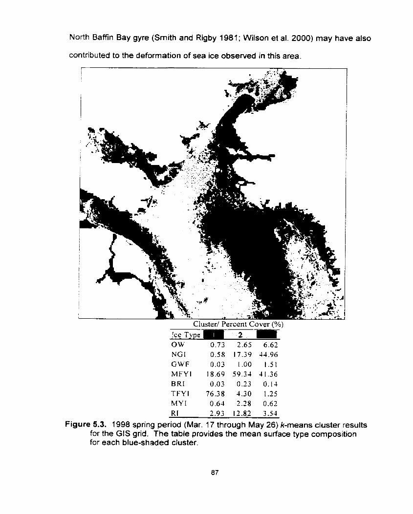
North Baffin Bay gyre (Smith and Rigby 1981; Wilson et al. 2000) may have also

contributed to the deformation of sea ice obsewed in this area.

Figure 5.3. 1998 spring period (Mar. 17 through May 26) k-means cluster results for the GIS grid. The table provides the mean surface type composition for each blue-shaded cluster.

SP cluster 3 was composed of low RI and MY1 concentrations relative to

cluster 2 (Fig. 5.3). The distribution was similar to clusters 3 and 4, substantiating

the interpretation of relatively low sea ice deformation towards Greenland and

Lancaster Sound. An exception of this similarity was observed within the Smith

Sound area. The presence of the Kane Basin ice bridge and the subsequent

large divergence of ice essentially masked the ability of a cluster analysis to

naturally separate the east and west sides of Smith Sound. However, the

previously discussed explanations of westward water mass movement and

induced upwelling was supported through the mean concentration distribution of

OW during the spring period (Fig. 5.4b). This result was in good agreement with

the location of warm water cells mapped by Steffen and Ohmura (1985), further

supporting their existence.

An additional area of very high open water concentrations just south of

Coburg Island was observed (Fig. 5.4a). Offshore winds and/or southward

currents and winds on either side of the island causing divergence of ice can

explain the location of the open water. Further, the ice divergence and

subsequent water mass movement could induce upwelling along the southern

edge of Coburg Island. Although no in-situ observations of water temperature

were made for this position during the spring perïod in 1998, Steffen (1985) did

find water temperatures to be above -1.8OC during both the 1978/ï9 and 1980/81

winters.

The 50 km transect demonstrated 65.3% surface cover c 30 cm thick (Table

6). As discussed above, the more extensive area of lower ice concentration was

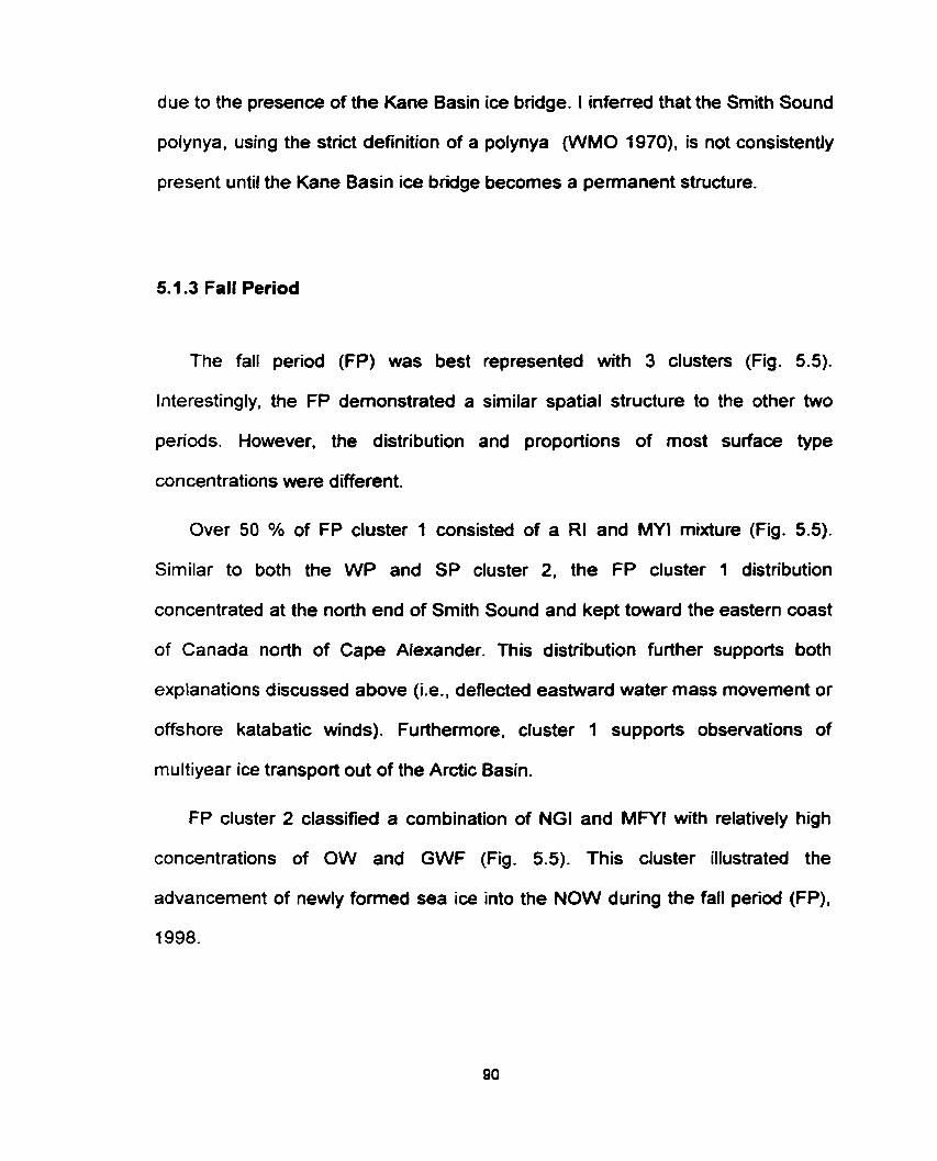
due to the presence of the Kane Basin ice bridge. I inferred that the Smith Sound

polynya, using the strict definition of a polynya (WMO 1970). is not consistently

present until the Kane Basin ice bridge becomes a permanent structure.

5.1.3 Fall Period

The fall period (FP) was best represented with 3 clusten (Fig. 5.5).

Interestingly, the FP demonstrated a similar spatial structure to the other two

periods. However, the distribution and proportions of most surface type

concentrations were different.

Over 50 % of FP cluster 1 consisted of a RI and MY1 mixture (Fig. 5.5).

Similar to both the WP and SP cluster 2, the FP cluster 1 distribution

concentrated at the north end of Smith Sound and kept toward the eastern coast

of Canada north of Cape Alexander. This distribution further supports both

explanations discussed above (i.e., deflected eastward water mass movement or

offshore katabatic winds). Furthemore, cluster 1 supports observations of

rnultiyear ice transport out of the Arctic Basin.

FP cluster 2 classified a combination of NGI and MFYI with relatively high

concentrations of OW and GWF (Fig. 5.5). This cluster illustrated the

advancement of newly fonned sea ice into the NOW during the fall period (FP),

1998.

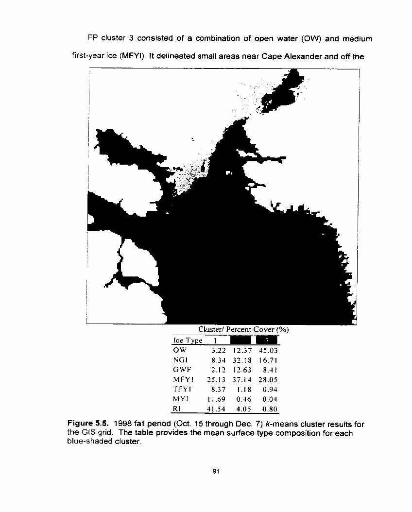
FP cluster 3 consisted of a combination of open water (OW) and medium

first-year ice (MFYI). ft delineated small areas near Cape Alexander and off the

Chster/ Percent Cover (%)

O W 3.22 12.37 45.03 NGI 8.34 32.1 8 16.71 G W F 2.12 12.63 8.41 MFYI 25.13 37.1 4 28.05 TFYI 8.37 1 . 1 8 0.94 iMY 1 1 1.69 0.46 0.04 RI 41-54 4.05 0.80

Figure 5.5. 1998 fall period (Oct. 15 through Dec. 7) k-means cluster results for the GIS grid. The table provides the mean surface type composition for each blue-shaded cluster.

southern tip of Coburg Island (Fig. 5.5). However, it was mainly distributed

towards the south end of the grid with an extension north along the west coast of

Greenland and into Whale Sound (Fig. 5.5). The southeastem portion was

predominately OW, whereas the southwestern portion of this distribution

consisted largely of MN1 (Fig. 5.6a and b, respectively). Prior to freeze-up, the

area was covered by 100% OW. Whereas, near the FP end (Le., December 7,

1998). sea ice nearly covered the whole region, with the exception of the

southwest Greenland coast. Barber et al. (2000) demonstrated predominant

southerly winds in this vicinity from 1979 to 1996. They also showed a late fall

accretion in the same vicinity. It was suggested that these winds could import

warmer air from southern Baffin Bay and could contribute to the late fall freeze-

up. Accordingly, the same mechanism is used to explain the open water

observed in this study. The influx of wanner air and/or warrner surface water from

southern Baffin Bay could impede ice formation and cause ice divergence.

Advection of this atmospheric andlor oceanic heat source may have reached

even further north. During the winter and spring periods, an area of relatively low

ice deformation was inferred along the Greenland coast between Whale Sound

and Cape York. Furthemore, high open water concentrations were observed

along this location for bath the spring and fall periods (Fig. 5.4b and 5.6a,

respectively). As a latent heat polynya mechanism is consistent with relatively

large surface forcing tbat causes ice divergence and deformation, the

observation of open water along this location implied the occurrence of a

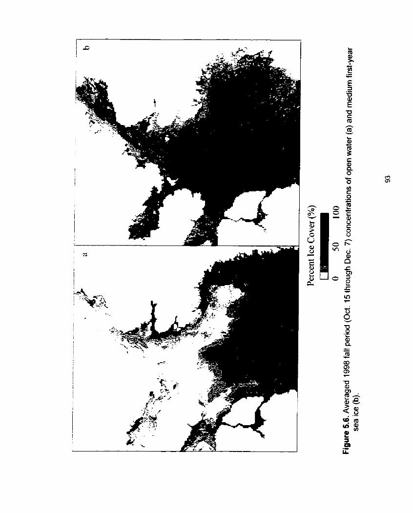
sensible heat input. The heat input could impede ice formation during freeze-up

resulting in a thinner ice cover, which would subsequently ablate earlier in the

spring. This mechanism was actually suggested, yet not explained, by Ito (1985).

During the fall period (FP). open water (OW) had higher concentrations

within and south of Whale Sound than north near Cape Alexander (Fig. 5.6a).

Furthermore, FP cluster 3 was largely absent in the vicinity of Smith Sound (Fig.

5.5). Smith Sound appears to be separated from the west Greenland coast south

of Whale Sound and hence the surface heat influx from south Baffin Bay (see

above) due to the presence of Northumberland Island and its neighboring islands

(Fig . 1.1 ). Consequently, the occurrence of a mechanism independent to the

explained upwelling along Smith Sound was inferred. This inference was

corroborated by an observed mode of late fall accretion and early spring ablation

(separate from the Smith Sound vicinity) along the Greenland coast from 1979 to

1996 (Barber et al. 2000).

The 50 km transect contained a composition of only 46.8% open w a t e r h

cover c 30 cm thick (Table 5.1). This was considerably less than Steffen's (1986)

observations, when averaged resulted in 91.4% open waterlice cover < 30 cm

(average obtained from December 2, 20 and 29, 1980 from Table IV; Steffen,

1986). As discussed earlier, the lower concentrations observed during this

investigation may have been the result of less sea ice congestion at the northem

end of Smith Sound than in Steffen's (1986) study.

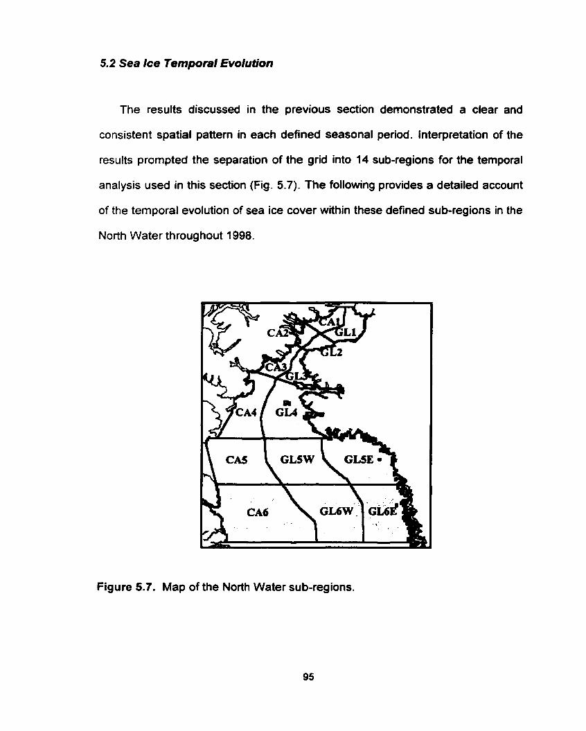
5.2 Sea /ce Temporal Evolution

The results discussed in the previous section demonstrated a clear and

consistent spatial pattern in each defined seasonal period. lnterpretation of the

results prompted the separation of the grid into 14 sub-regions for the temporal

analysis used in this section (Fig. 5.7). The following provides a detailed account

of the temporal evolution of sea ice cover within these defined sub-regions in the

North Water throughout 1998.

Figure 5.7. Map of the North Water sub-regions.

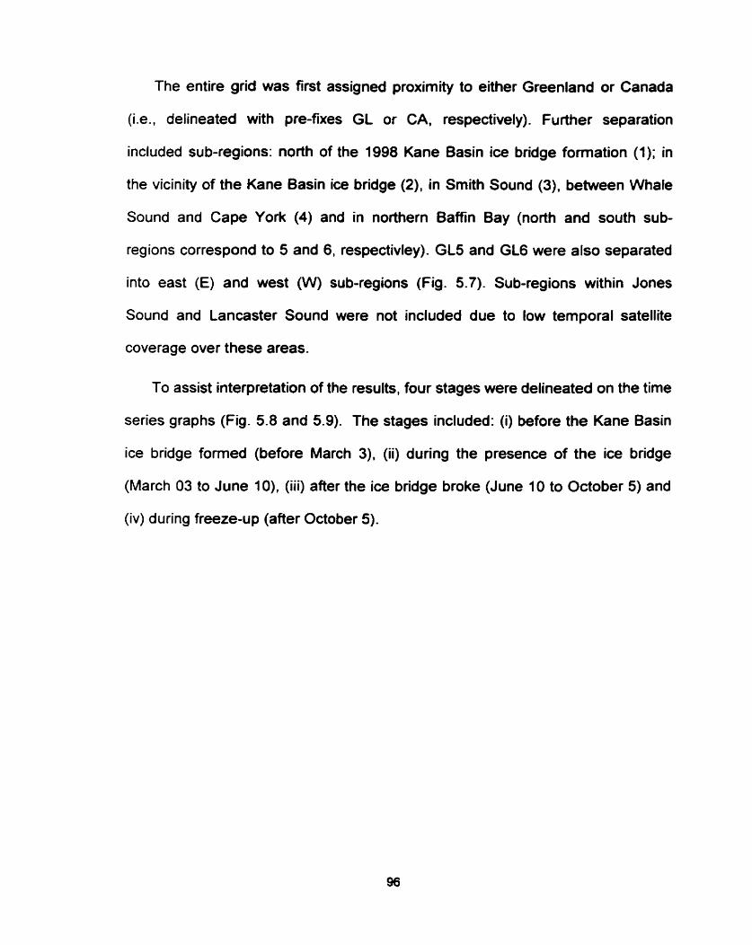
The entire grid was first assigned proximity to either Greenland or Canada

(i.e., delineated with pre-fixes GL or CA, respectively). Further separation

included sub-regions: north of the 1998 Kane Basin ice bridge formation (1); in

the vicinity of the Kane Basin ice bridge (2), in Smith Sound (3). between Whale

Sound and Cape York (4) and in northern Baffin Bay (north and south sub-

regions correspond to 5 and 6, respectivley). GL5 and GL6 were also separated

into east (E) and west (W) sub-regions (Fig. 5.7). Sub-regions within Jones

Sound and Lancaster Sound were not included due to low temporal satellite

coverage over these areas.

To assist interpretation of the results, four stages were delineated on the time

series graphs (Fig. 5.8 and 5.9). The stages included: (i) before the Kane Basin

ice bridge forrned (before March 3). (ii) during the presence of the ice bridge

(March 03 to June 1 O), (iii) after the ice bridge broke (June 10 to October 5) and

(iv) during freeze-up (after October 5).

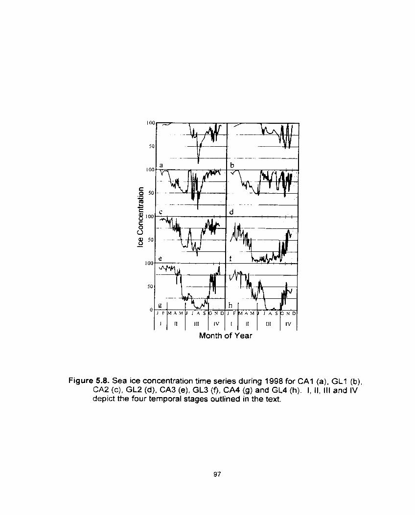
Month of Year

Figure 5.8. Sea ice concentration time series during 1998 for CA1 (a), GL1 (b), CA2 (c), GL2 (d), CA3 (e), GL3 ( f ) . CA4 (g) and GL4 (h). 1 , 11 , III and IV depict the four temporal stages outlined in the text.

Month of Year

Figure 5.9. Sea ice concentration time series during 1998 for CA5 (a), GLSW (b). CA6 (c), GL6W (d), GL5E (e) and GL5E (f). 1, 11, III and IV depict the four temporal stages outlined in the text.

5.2.1 Prior to Ice Bridge

Prior to formation of the Kane Basin ice bridge, the North Water (NOW) sea

ice is advected continually from the Lincoln Sea into Baffin Bay. North of Cape

York, sea ice concentrations were close to but slightly below 100%

concentrations due to the consistent motion of the pack-ice and subsequent

crack and lead formation (Fig. 5.8). South of Cape York, the pack within Baffin

Bay had a more compact distribution and did not demonstrate the lower ice

concentrations (Fig. 5.9).

Greenland sub-regions between Smith Sound and Cape York (i.e.. GL3 and

GL4) both dernonstrated average sea ice concentrations less than 75% prior to

the ice bridge formation (Fig. 5.8). As discussed earlier, these results can be

explained through either coastal upwelling (Steffen 1985) or by offshore katabatic

winds that have been modeled to occur along the coast of these sub-regions

(Bromwich et al. 1996). 1 note again that no observations of ocean surface

temperature were made in this vicinity during the expedition.

5.2.2 Ice Bridge Present

Once the bridge formed, sea ice cover north of the bridge (Le., CA1 and

GL1) became landfast and demonstrated near 100% concentrations (Fig. 5.8). In

the vicinity of the bridge and Smith Sound, the latent heat mechanism was

dominant. Ice concentrations dropped slightly then stabilized at a point where air

temperatures, winds and/or currents were balanced by newly formed sea ice that

accumulated at the southern extent (Fig. 5.8). This process is typical of a latent

heat polynya mechanism such as described by Pease (1987).

The polynya opened rapidly in May (Fig. 5.8). From April 29, 1998, the air

temperature increased frorn approximately -1 1 to -1 -1 OC by May 2, leveled off at

an averaged -5OC until May 8 where it decreased to -12.2OC on May 12, then

steadily increased to approximately O°C by the end of May (Minnett 2000; Fig.

5.10). Further, 3 strong peaks of winds coming from the north (i.e.. near 01360°)

occurred throughout May (Minnett 2000; Fig. 5.1 O). During this period I speculate

that a positive feedback loop was created. Wanner temperatures resulted in less

new ice formation and higher winds resulted in more stress on the polynya's

southern ice extent. This resulted in more open water, which absorbed greater

amounts of solar energy and provided a longer north-south fetch for wave

development. The increased absorption and wave stress would cause increased

lateral and mechanical sea ice ablation (e-g. Hall and Rothrock 1985). All of

these factors would feedback into creating a larger open water area in the NOW.

Within Smith Sound, a substantial difference was observed betweeo average

ice concentrations of CA3 and GL3 (Fig. 5.8). Both sub-regions showed a slight

decreasing trend after the formation of the ice bridge. Once the polynya began to

open in May, ice concentrations in GL3 dropped to less than 15% (Fig. 5.8). The

low concentrations were attributed to a small amount of landfast ice along the

Greenland coast in this vicinity. The lower landfast concentration in GL3 was due

to the offshore movement of water described above. Further, sensible heat inputs

from upwelling along the Greenland coast may have also contributed to the lower

ice concentrations observed in GL3.

In GL4, the extensive opening of the polynya was not as dramatic as

compared with CA4 (Fig. 5.8). This was attributed to the direction of sea ice

motion in this area. Wilson et al. (2000) dernonstrated that sea ice moves

northward in this region as a consequence of the north Baffin Bay gyre.

Consequently, ice was advected into this sub-region as opposed to being

exported southward.

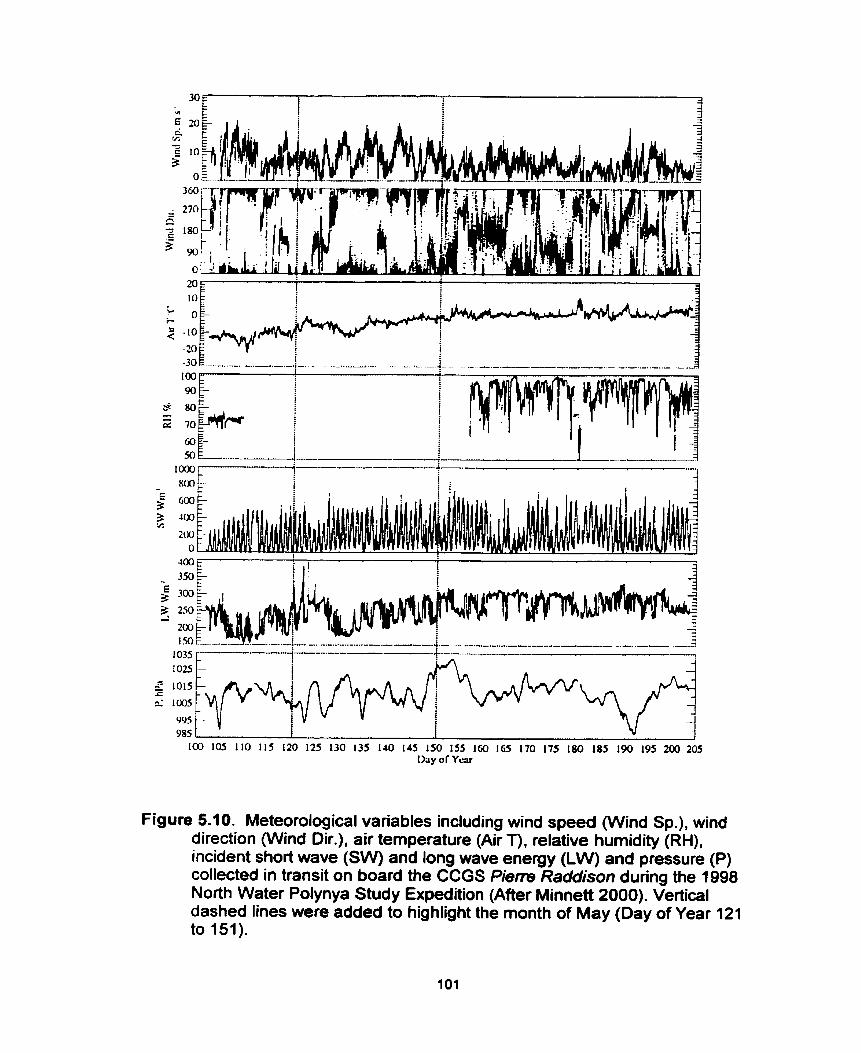
xcn L- i . i

Figure 5.1 0. Meteorological variables including wind speed Wind Sp.). wind direction (Wind Dir.), air temperature (Air T), relative humidity (RH), incident short wave (SW) and long wave energy (LW) and pressure (P) collected in transit on board the CCGS Pierre Raddison during the 1998 North Water Polynya Study Expedition (After Minnett 2000). Vertical dashed lines were added to highlight the month of May (Day of Year 121 to 151).

5.2.3 After Ice Bridge

After the ice bridge broke, sea ice ernptied through Kane Basin and into the

NOW in a strong pulse. This pulse was observed as a decrease in CA1 and GL1

ice concentrations and subsequent increases in sub-regions to the south (Fig.

5.8). The pulse of sea ice was not observed in GL3, as ice did not flow through

this sub-region (Fig. 5.8). The sea ice was essentially pushed towards the

Canadian side of Smith Sound due to the offshore water mass movernent

described above. As rnentioned above, the increase in sea ice concentrations in

GL4 was due to an increased import of sea ice from the south (Wilson et al.

2000).

Within CA4, the sea ice pulse was greatly diminished and south of Cape

York the pulse of sea ice was not observed (Fig. 5.8 and 5.9, respectively).

Furthermore, throughout July, August and September. sea ice was continually

observed to flow though Kane Basin. However, the sea ice appeared to ablate

before it reached Cape York. The ablation of sea ice in this region was probably

accentuated by lateral melt and mechanical erosion from the open ocean (e-g..

Hall and Rothrock 1985).

During August and September, sea ice concentrations increased within Kane

Basin and CA3 (Fig. 5.8). The increase was attributed to increased ice flowing

into the area from the north. During this time, temperatures had cooled enough to

slow the ablation of sea ice.

5.2.4 Fall Freeze-up

Fall freeze-up began in mid October (determined from ScanSAR imagery).

The accumulation of newly formed sea ice combined with the influx of ice from

the north was observed throughout the whole region (Fig. 5.8 and 5.9). Nearly al1

sub-regions demonstrated ice concentrations increasing to values close to that

observed in January, with the exception of GL4 and GLGE.

GL6E can be explained by predominate southerly winds observed in the area

along the Greenland coast (Barber et al. 2000). As explained in section 5.1. the

southerly winds could import w a n atmospheric air masses andior warm surface

water from southern Baffin Bay, irnpeding ice formation in the local area.

Similarly, GL4 can be explained by the same influx of wamer air temperatures

andior surface water. in addition to offshore ice divergence.

5.3 Mixed Layer Depth ( M D ) and Sea /ce Patterns

The mixed layer refers to the ocean's surface layer where density is relatively

homogeneous throughout. This layer rests on top of a themocline or halocline

through which water density increases dramatically due to a decrease in

temperature or an increase in salinity, respectively. A shallow mixed layer depth

(MLD) is vital for the entrainment of phytoplankton populations to the surface

where they can benefit ftorn non-limiting irradiance. The following compares

mixed layer depths measured during the NOW study 1998 campaign with sea ice

cover in the North Water.

Legs1 (March 26 to May 5, 1998) and 2 (May 5 to June 2, 1998) both

demonstrated relatively deep MLDs with large ranges (Fig. 5.11a and b,

respectively). Their averages (îsd) were 56134 and 37I22 m, respectively.

During Leg 1, deep (up to 157 m) MLDs were observed along the eastern

Ellesmere Island coast and shallow (10 to 20 m) MLDs off the coast of Cape

Alexander and surrounding the Carey Islands (Fig. 5.11a). During Leg 2. a

similar pattern was observed with shallow MLDs along the Greenland coast and

deeper MLDs toward the Canadian coast. There was also a general trend of

shallower MLDs toward the southeast of the region (Fig. 5.1 1 b).

Throughout April and May (i.e., Legs 1 and 2). northerly winds and

temperatures increased resulting in the extensive opening of the NOW polynya.

Areas with deep MLDs along the Greenland coast were generally covered by ice,

whereas some of the areas with deep MLDs along the Ellesmere Island coast

were ice free. A dynamic ice cover was inferred along the Ellesmere Island coast.

This was indicative of a latent heat polynya mechanism acting to keep the area

ice free. Subsequently, although the area was ice free, the dynamic surface

conditions would act to keep a relatively deep MLD. Alternatively, areas with

shallow mixed layer depths along the Greenland coast corresponded to inferred

areas of lower ice deformation. It was suggested that either atmospheric andlor

oceanic heat was imported from southern Baffin Bay. Further, Yackel et al.

(2000) observed melt onset dates to occur first along the southeastern edge of

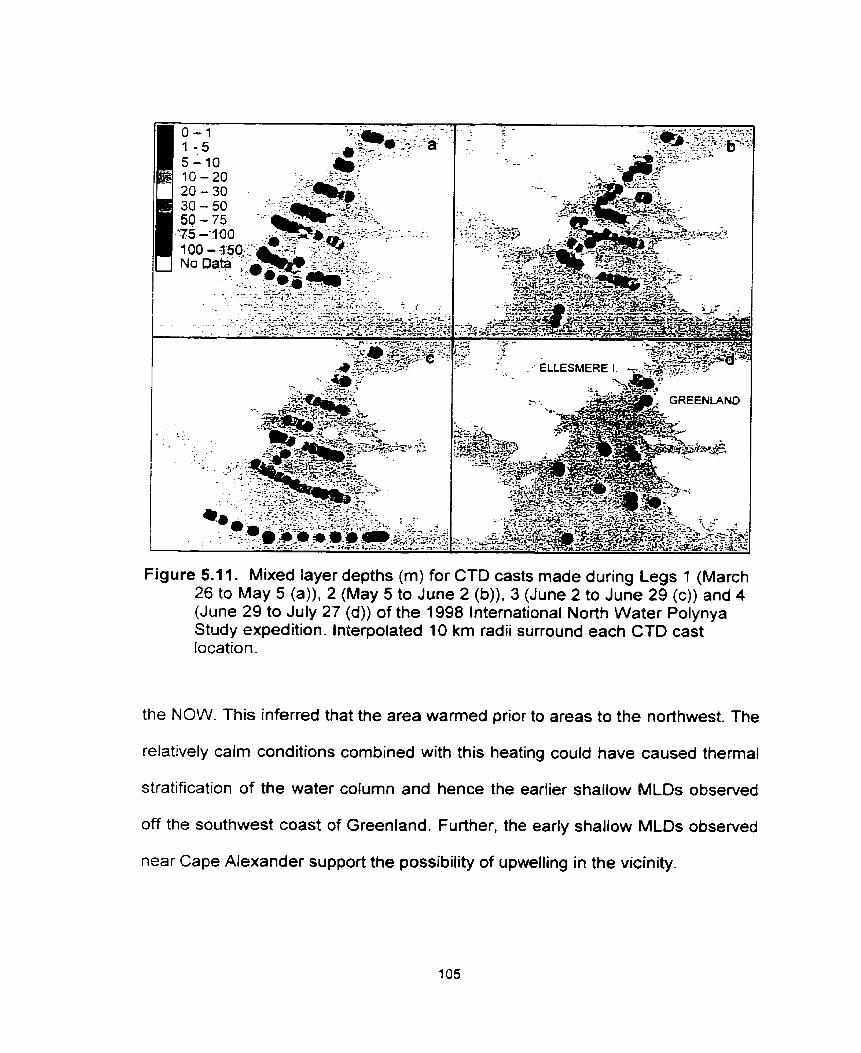
Figure 5.1 1. Mixed layer depths (m) for CTD casts made during Legs 1 (March 26 to May 5 (a)), 2 (May 5 to June 2 (b)). 3 (June 2 to June 29 (c)) and 4 (June 29 to July 27 (d)) of the 1998 International North Water Polynya Study expedition. lnterpolated 10 km radii surround each CTD cast location.

the NOW. This inferred that the area warrned prior to areas to the northwest. The

relatively calm conditions combined with this heating could have caused thermal

stratification of the water cofumn and hence the earlier shallow MLDs observed

off the southwest coast of Greenland. Further, the early shallow MLDs observed

near Cape Alexander support the possibility of upwelling in the vicinity.

By Legs 3 (June 2 to June 29) and 4 (June 29 to July 27), MLDs were

shallow throughout the NOW (Fig. 5.11 c and d, repectively). with averages of

12î6 and d i 3 mm, respectively. During these periods. sea ice was ablating

extensively. Therefore, the low salinity melt water may have acted to stratify the

waters, even in areas of high surface deformation as inferred along the

Ellesmere Island coast.

In this chapter I have described the results of the spatio-temporal ice cover

analysis for the NOW and related it to potential physical mechanisms responsible

for the observed patterns. I also discussed the relationship between mixed layer

depth observations and the interpreted ice cover results. In the next chapter I

provide the conclusions drawn from chapters 4 and 5 and recommendations as

to how this data set can be further examined.

CEIAPTER 6: CONCLUSIONS AND RECOMMENDATIONS

The objectives of this thesis have been: (1) To develop a robust ScanSAR

sea ice classification scheme; (2) To examine the spatial and temporal patterns

of sea ice cover within the North Wate: (NOW) in relation to the potential physical

mechanisms responsible for the NOW polynya's occurrence. and (3) To relate

the sea ice spatio-temporal patterns to the potential for biological productivity

within the NOW. ln this chapter I conclude on the examination of these objectives

and recommend future directions for the use of the data set created as part of

this thesis.

To meet the first objective of this thesis I developed a hierarchical sea ice

classification scheme using over 150 RADARSAT-1 ScanSAR images. The

classified ice types were then structured into a Geographic Information Systern

(GIS) framework for subsequent analysis pertaining to my second and third

thesis objectives.

To meet my second objective I examined the spatial and temporal patterns of

sea ice cover within the North Water (NOW) in relation to the potential physical

mechanisms responsible for the resident polynya's occurrence. Ice conditions

demonstrated a clear and consistent spatial structure in the NOW for the winter

(WP), spring (SP) and fall (FP) periods of 1998. The consistency of the spatial

patterns of sea ice was somewhat surprising but illustrated the strength of sea

ice as a proxy indicator of the polynya formation and maintenance processes.

An area of high ice deformation (Le., high rubble ice concentrations) was

observed along the Canadian Coast. inferring strong winds andlor currents,

which would be consistent with a latent heat polynya mechanisrn. The

composition of thick multiyear and rubble ice within the dynamic region also

represented a previously poorly documented contribution to the freshwater flux

from the Arctic Basin into Baffin Bay. Opposite to the dynamic area along the

eastern Canadian coast, a relatively less dynamic ice environment was inferred

along the Greenland coast. As open water was observed along the Greenland

coast in early spring and late fall. a sensible heat mechanism was suspected.

Through Smith Sound, tight distributions of thick ice along the Canadian

coast and thin ice types and open water along the less dynamic Greenland coast

supported Steffen's (1985) explanation for the existence of a sensible heat input

at this location. Steffen's rationale suggested that without the existence of an ice

edge combined with ice divergence due to winds andior currents there would be

no upweiling of warm Baffin Bay Atlantic water. The location of high open water

concentrations observed consistently off the coast of Coburg Island combined

with Steffen's (1985) observation of warm water at this location suggests that this

mechanism may occur in more than one location within the NOW. An alternative

explanation of offshore katabatic winds causing ice divergence off the Greenland

coast in the Smith Sound vicinity was also suggested. Similar to Steffen's (1985)

explanation, offshore transport of water could induce upwelling of relatively wam

Baffin Bay Atlantic water. However, the latter mechanism would be less

dependent on the congestion of ice within Kane Basin.

An exception to the spatial trend described above was observed off the coast

of Greenland south of Cape York. Relatively high mean rubble ice (RI)

concentrations throughout the winter (WP) and spring (SP) periods and open

water during the fall period (FP) were observed along this location. These

observations were explained by contributions of the West Greenland surface

current and predominate southerly winds.

Additionally, large expanses of open water were observed along the

Greenland coast between Whale Sound and Cape York during the SP and FP. It

was suggested that a surface influx of atmospheric and/or oceanic heat from

south Baffin Bay could explain the open water. This would result in a thinner ice

cover causing an earlier spring ablation than surrounding areas. It was also

inferred that this sensible heat input was independent of the mechanism

occurring through Smith Sound.

Compared to similar observations made by Steffen (1986) for the winter of

1980181, substantially less open water was observed within Smith Sound during

1998. This was explained in part by the composition of sea ice at the northern

entrance to Smith Sound. Kane Basin prior to and after ice bridge formation was

noted to consist of very thick multiyear ice of Arctic Basin origin. I speculated that

large multiyear ice floes could contribute to congestion of sea ice at the head of

Smith Sound.

Ito and Müller (1977), during the years of 1974 and 1975, observed the Kane

Basin ice bridge to be composed of thickly ridged MY1 with ice elevations up to 5

m above sea level. Similar observations were made during the International

North Water Polynya Study 1998 campaign (personal observation). Multiyear ice

is much stronger and more rigid than first-year ice due both to its higher

freshwater content and thickness (Weeks and Ackley, 1986). Consequently, MY1

may provide extra structural support against the consistently strong northerly

winds and southward currents through Smith Sound than would FYI acting alone.

That is, smaller and thinner multiyear ice floes would result in a lower probability

of sea ice congestion at the head of Smith Sound and a later formation of the

Kane Basin ice bridge. Such a scenario is also in accordance with observed

trends of decreasing Arctic pack-ice extent (Parkinson et. al. 1999) and volume

(Rothrock et. al. 1999). A historical analysis of the annual bridge formation further

suggested that the ice bridge formation has become less consistent in the 1990's

versus the 1980's (Barber et al. 2000). Consequently, observations of ice

congestion and bridge formation within Kane Basin may act as a proxy indicator

of climate change andlor variability.

Evolution of sea ice in the North Water (NOW) during 1998 provided

additional insight into the physical mechanisrns that act to form and maintain the

polynya. The polynya appeared to be largely controlled by the latent heat

mechanism. Pnor to the ice bridge formation and during fall freeze-up, there were

some open water areas along the coast of Greenland that could also be

explained, at least in part, through sensible heat inputs (Le., both oceanic and

atmospheric). However, no observations were made to prove or disprove the

input of sensible heat in the NOW.

During May, nearly hivo months after the ice bridge fomed, the polynya

opened rapidly as a result of a positive feedback loop on ice ablation. The

feedback was initiated through increased wind speeds and temperatures. The

feedback involved increasing lateral and mechanical ablation processes as a

result of an increasing open water area. Once the NOW was completely open,

the resultant open ocean conditions caused imported sea ice to locally ablate

throughout the summer months.

In objective three I began the process of examining the relationship between

physical processes (particularly those relating to sea ice) and their biological

conseq uences. In particular I examined the relationship between sea ice spatio-

temporal patterns and the observed mixed layer depths (MLDs). The occurrence

of a shallow MLD is usually consistent with the occurrence of a primary

production bloom in polar waters (e-g., Maynard and Clark 1987). A qualitative

cornparison made between mixed layer depth (MLD) and sea ice spatio-temporal

patterns demonstrated a relationship based on ice defonnation. Generally, in

areas of lower inferred ice defomation (i.e., off the coast of Greenland), shallow

MLDs were observed earlier with the exception of ice-covered waters. It

appeared that high surface turbulence from either atmospheric or ocean stress

was responsible for slowing the development of shallow MLDs along the

Canadian coasts. With earlier shallow MLDs, a subsequent early pnmary

production bloom could occur due to non-iimiting irradiance. Therefore,

consistent with Lewis et al. (1996) primary producen would first bloom along the

Greenland coast where growth conditions were first favorable. Further, the MLDs

observed throughout the North Water in June were indicative that the entire

region could support an early prirnary production bloom relative to surrounding

ice-covered areas.

It should be noted that without upwelling the bloom would be short lived due

to nutrient depletion. It was suggested in the NOW proposal (1997) that not only

an early bloom may occur, but an extended bloom as well. This suggestion was

made as a rectification for the rich wildlife found along the adjacent coasts of the

NOW. The occurrence of upwelling was not observed with the data used in this

thesis and therefore conclusions could not be made. Similarly, no convincing

evidence of upwelling was made during the oceanographic portion of the NOW

study (Melling et al. 2000). However, the results of this thesis highlight areas of

open water that could be explained, at least in part, through the occurrence of

upwelling. Consequently, whether an extended bloom occurs in the NOW and itr;

relationship to the physical polynya mechanism have yet to be confirmed. This

may be done through a more detailed quantitative analysis of these data, or

perhaps a future study of the North Water with a focus on the areas where

upwelling rnay occur (Le., the southeastern portion of the NOW and off the

coasts of Cape Alexander and Coburg Island) may be warranted.

This thesis documented the creation of a high-resolution (both temporal and

spatial) GIS database of sea ice type and concentration. The database was

created to examine the response of the sea ice to atmospheric and oceanic

forcing iind to relate sea ice processes to biological production. The results

presented in this thesis represent only the first-order approximation of these

processes. Biologists, geographers and oceanographers involved in the NOW

study are just beginning to rnake use of the GIS database developed here.

Further research will develop ideas of ocean-sea ice-atmosphere processes and

further determine the biological and physical interrelationships that exist within

the NOW. I recommend the following studies be conducted as a natural evolution

of this thesis:

1. A regional surface energy balance study through the use of sea ice

cover and modeled atmospheric parameters interpolated to the GIS

grids. The model results are being interpolated with weighting on

observed ice types and concentrations and surface climate

measurements made from ship and on the fast ice during the

International North Water Polynya Study 1998 campaign;

2. A sea ice flux study through the combination of surface type, sea ice

motion (see Wilson et al. 2000), sea ice deformation and

accretionlablation (obtained from a sea ice themodynamic model)

each interpolated to the GIS grid. The results will be used to estimate

the sea ice budget for the entire 1998 year as well as compare with

physical and biological processes occurring within the NOW.

3. A statistical cornparison between results obtained through different

data sources including ice concentration from the GIS grid, the Special

Sensor Microwave Imager (SSMII) and the Advanced Very High

Resolution Radiometer (AVHRR). This will allow us to improve course

spatial resolution estimates of sea ice type and concentration and thus

provide better historical analysis of the NOW ocean-sea ice-

atmosphere processes.

The recommendations above, and the thesis results presented here

represent progress in the development of our understanding of ocean-sea ice-

atmosphere processes that occur within the North Water Polynya. The combined

results from the first series of journal papers will be forthcoming in a special issue

of the journal 'Atrnosphere-Ocean'. Presented in this special issue is evidence for

the fact that the NOW polynya cm. and does. respond to climate variability and

change. Linking the biological consequences of this change will continue in

ongoing analysis of the NOW research network building upon the results in my

thesis.

Aagaard, K. and E.C. Carmack. 1989. The role of sea ice and other freshwater in the Arctic circulation. J. Geophys. Res., 94: l4,485-Ml498.

Agnew, T. A., 1998. Drainage of multiyear ice from the Lincoln Sea. Can. Metero. Oceanogr. Soc. Bull. 26: 1 0 1 -1 03.

Alexander, V. 1994. Primary productivity regimes of the neanhore Beaufort Sea, with reference to the potential role of sea ice biota. IN, The Coats and Shelf of the Beaufort Sea. J-C. Reed and J.E. Sater (Eds). Arctic lnstitute of North America, Arlington, VA. pp. 604-635

Alexander, V. and H.J. Niebauer. 1981. Oceanography of the eastern Bering Sea ice-edge zone in spring. Limnol. Oceanogr., 26: 1 1 1 1-1 126.

Anderberg , M. R. 1 973. Cluster Analysis for Applications. Proba bility and Mathematical Statistiw: A Series of Monographs and textbooks, Birnbaum, Z.W. and E. Lukacs (Eds). Academic Press, Inc., New York. 359 pp.

Barber, DG. and E.F. LeDrew. 1991. SAR sea ice discrimination using texture statistics: A multivariate approach. Photogramm. Eng. Remote Sens.. 57: 385-395.

Barber, D.G., D.D. Johnson and E.F. LeDrew. 1991. Measuring climatic state variables from SAR images of sea ice: The SlMS SAR validation site in Lancaster Sound. Arctic, 44: 108-1 21 .

Barber, D.G., M.E. Shokr, R.A. Fernandes, E.D. Soulis, D.G. Flett and E.F. LeDrew. 1993. A cornparison of second-order classifien for SAR sea ice discrimination. Photogramm. Eng. Remote Sens., 59: 1 397-1 408.

Barber, DG., T.N. Papakyriakou, E.F. LeDrew and M.E. Shokr. 1995. An examination of the relation between the spring period evolution of the scattering coefficient (oO) and radiative fluxes over land fast sea-ice. Int. J. Remote Sensing, 16: 3343-3363.

Barber, D.G. and S.V. Nghiem. 1999. The role of snow on the thermal dependence of rnicrowave backscatter over sea ice. J. Geophys. Res., 104: 25,789-25,803.

Barber, DG., J. Hanesiak and J. Piwowar. Sea ice - atmosphere processes within the North Water polynya (NOW): Part 1 - Seasonal and annuaf averages between 1979 and 1996. A-O, In Review 2000.

Barry, R.G., M.C. Serreze, J.A. Maslanik, and R.H. Preller. 1993. The Arctic Sea Ice-Climate System: Observations and Modelling. Rev. Geophys., 31: 397422.

Bauer, J. and S. Martin. 1983. A model of grease ice growth in small leads. J. Geophys. Res., 88: 29 1 7-2925.

Bel'chanskiy, G.I., D.C. Douglas and N.N. Kozlenko. 1996. Assessrnent of sea- ice conditions using two-channel active and passive microwave systems. Polar Geog. 20: 294-305.

Bishop, Y.M.M., S.E. Fienberg and P.W. Holland. 1975. Discrete Multivanate Analysis: Theory and Practice. MIT Press, Cambridge.

Boertman, O. and A. Mosbech. 1998. Distribution of the little Auk (Alle alle) breeding colonies in Thule district, northwest Greenland. Polar Bio., 19: 206-2 1 O.

Bourke, R.H. and R.G. Paquette. 1991. Formation of Baffin Bay bottom and deep waters. IN Deep Convection and Deep Water Formation in the Oceans, P.C. Chu and J-C. Gascard (Eds), Elsevier, Amsterdam, pp. 135- 155.

Bromwich, D.H., Y. Du and K. M. Hines. 1996. Wintertime surface winds over the Greenland Ice Sheet. Mon. Wea. Rev., 124: 1941-1947.

Brown, R.G.B. and D.N. Nettleship. 1981. The biological significance of polynyas to Arctic colonial seabirds. IN, Polynyas in the Canadian Arctic, Stirling, 1. and H. Cleator. (Eds) Canadian Wildlife Service, Ottawa (Occasional Paper No. 45.), pp. 59-65.

Carmack. E.C. 1990. Large-scale physical oceanography of polar oceans. IN. Polar Oceanography Part A: Physical Science, W.O. Smith (Ed) , Academic Press, New York, pp. 171 -21 1.

Comiso, J.C., C.R. McClain, C.W. Sullivan, J.P. Ryan and C.L. Leonard. 1993. Coastal Zone Color Scanner pigment concentrations in the southem ocean and relationships to geophysicai surface features, J. Geophys. Res., 98: 24 1 9-245 1.

Darby, M.S., A.J. Willmott and L.A. Mysak. 1994. A nonlinear steady-state model of the North Water polynya. Baffin Bay. J. Phys. Oceanogr., 24: 101 1-1020.

De Bastiani, P. 1990. Canadian Arctic Manne Ice Atlas - Wlnter 1987/88 with Perspectives fmm l98W87 and l98B/B9. Canarctic Shipping Company Limited, Ottawa, ON, 116 pp.

Dunbar, M.J. 1969. The geophysical position of the North Water. Arctic, 22: 438-441.

Dunbar, M.J. 1981. Physical causes and biological significance of polynyas and other open water in sea ice. IN, Polynyas in the Canadian Arctic, Stirling, 1. and H. Cleator. (Eds) Canadian Wildlife Service, Ottawa (Occasional Paper No. 45.), pp. 2943.

Dunbar, M. and M.J. Dunbar. 1972. The history of the North Water. Pmc. R.S.E. (B), 72: 231-241.

Finley, K.J. and W.€. Renaud. 1980. Marine mammals inhabiting the Baffin Bay North Water in winter. Arctic, 33: 724-738

Gosselin, M. and L. Legendre. 1990. Light and nutrient limitation of sea-ice microalgae (Hudson Bay, Canadian Arctic). J. Phycol. 26: 220-232.

Hall, R.J. and D.A. Rothrock. 1987. Photogammetric observations of the lateral melt of sea ice floes. J. Geophys. Res., 92: 7045-7048.

Haralick, R.M., K. Shanmugan and I. Dinstein. 1973. Textural features for image classification. IEEE Trans. Sys. Man Cybemet., 3, no. 6,610-621.

Haverkamp, D. and C. Tsatsoulis. 1999. Information fusion for estimation of summer MIZ ice concentration from SAR imagery. IEEE Tram Geosci. Remote Sens., 37: 1 278-1 29 1 .

Hirche, H.-J., M.E.M. Baumann, G. Kattner and R. Gradinger. 1991. Plankton distribution and the impact of copepod grazing on primary production in Fram Strait. Greenland Sea. J. Mar. Syst.. 2: 477494.

Holrnes, Q.A., D.R. Nuesch and R.A. Shuchman. 1984. Texturaf analysis and real-time classification of sea-ice types using digital SAR data. IEEE Trans. Geosci. Remote Sens., 22: 1 1 3- 1 20.

Holst, M. and 1. Sirling. 1999. A note on sightings of bowhead whales in The North Water Polynya, Northern Baffin Bay, May-June, 1998. J. Cetacean Res. Manage. 1 : 153-1 56.

IAPP. 1 989. International Arctic Polynya Program. Arctic Ocean Sciences Board. lnstitute of Marine Sciences, University of Fairbanks, Alaska. 99775-1080. 28 pp.

ito. H. 1985. Decay of the sea ice in the North Water area: observation of ice cover in Landsat imagery. J. Geophys. Res., 90: 8 1 02-8 1 1 0.

Ito, H. and F. Müller. 1977. Horizontal movement of fast ice in the North Water area. J. Glaciol., 19: 547-554.

Ito, H. and F. Müller. 1982. Ice Movement through Smith Sound in northern Baffin Bay, Canada, observed in satellite imagery. J. Glaciol. , 28: 129- 143.

Kwok, R., E. Rignot, B. Holt, and R. Onstott. 1992. Identification of sea ice types in spaceborne synthetic aperture radar data. J. Geophys. Res., 97: 2391 - 2402.

Lewis, E.L., D. Ponton, L. Legendre and B. LeBlanc. 1996. Springtime sensible heat, nutrients and phytoplankton in the Northwater Polynya, Canadian Arctic. Cont. Shelf Res., 16: 1775-1 792.

Livingstone, C.E., R.G. Onstott, L.D. Arsenault, A.L. Gray and K.P. Singh. 1987. Microwave ice signatures near the onset of melt. IEEE Trans. Geosci. Remote Sens., 25: 1 74-1 87.

MANICE. 1994. Manual Standard Procedures for Observing and Repoding Ice Conditions 8M edition. Ice Services Branch, Atrnospheric Environment Service, Ottawa, ON.

Manly, B.F.J. 1986. Multivariate Statistical Methods. Chapman and Hall, London.

Marceau, D.J., P.J. Howarth, 3.-M. M. Dubois and D.J. Gratton. 1990. Evaluation of the grey-level CO-occurrence rnatrix method for land-cover classification using SPOT imagery. lEEE Trans. Geosci. Remote Sens., 28: 513-519.

Martin, S., R. Drucker and M. Fort. 1995. A laboratory study of frost fiower growth on the surface of young sea ice. J. Geophys. /?es.. 100: 7027- 7036.

Massom, R.A. 1988. The biological significance of open water within the sea ice covers of the polar regions. Endeavour, New Series, 12: 21 -27.

Maykut, G A . 1978. Energy exchange over young sea ice in the central Arctic. J. Geophys. Res., 83: 3646-3658.

Maykut, G A . 1982. Large-scale heat exchange and ice production in the central Arctic. J. Geophys. Res., 87: 7971 -7984.

Maykut, G.A. and T.C. Grenfell. 1975. The spectral distribution of light beneath first-year sea ice in the Arctic Ocean. Limnol. Oceanogr., 20: 554-563.

Maynard, N.G. and D.K. Clark. 1987. Satellite color observations of spring blooming in Bering Sea shelf waters during the ice edge retreat in 1980, J. Geophys. Res., 92: 71 27-71 39.

McBean, G. 1992. The Earth's climate system. WMO Bull.. 41: 393-401.

McLaren, AS. 1988. Analysis of under-ice topography in the Arctic Basin as recorded by the USS Nautilus during August 1958. Arctic, 41 : 1 17-1 26.

Melling, H., Y. Gratton and G. Ingram. Oceanic circulation within the North Water polynya in Baffin Bay. A-O, In Review 2000.

Minnett, P.J. Meteorological conditions in the North Water Polynya: spring and summer, 1998. A-O, In Review 2000.

Muench, R.D. 1971. The physical oceanography of the northern Baffin Bay region. IN The Bafin Bay-North Water Pmject Repod 7. Arctic Institute of North America, Calgary, 150 pp.

Muench, R.D. and H.E. Sadler. 1973. Physical oceanographic observations in Baffin Bay and Davis Strait. Arctic, 26: 73-76.

Mundy, C.J. and DG. Barber. On the relationship between the temporal evolution of sea ice spatial patterns and the physical mechanisms creating and maintaining the North Water polynya. A-O, In Review March 2000.

Mysak. L.A. and F. Huang. 1992. A latent- and sensible-heat polynya model for the North Water, northern Baffin Bay. J. Phys. Oceanogr., 22: 596-608.

Nettleship, D.N. and P.G.H. Evans. 1985. Distribution and status of the Atlantic Alcida. IN, The Atlantic Alcidae, D.N. Nettleship and T.R. Birkhead (Eds), Academic Press, London, Pp. 53-1 54.

Nghiem, S.V., S. Martin, D.K. Perovich. R. Kwok, R. Drucker and A.J. Gow. 1997. A laboratory study on the effect of frost flowers on C band radar backscatter from sea ice. J. Geophys. Res., 102: 3357-3370.

Niebauer, H.J. and W.O. Smith. 1989. A numerical mode1 of mesoscale physical-biological interactions in the F ram Strait marginal ice zone. J. Geophys. Res., 94: 16,151 -16.175.

Nutt, D.C. 1969. The North Water of Baffin Bay. Polar Notes, 9: 1-25.

Nystuen, J.A. and F.W. Garcia. Jr. 1992. Sea ice classification using SAR backscatter statistics. IEEE Trans. Geosci. Remote Sens., 30: 502-509.

NOW (International North Water Polynya Study) Proposal. 1997. University of Laval, GIROQ, ftp://kestrel.fs~.ulaval.ca/home/qÏroq/now/. 70 pp.

Parkinson, CL., D.J. Cavalieri, P. Gloersen, H.J. Zwally and J.C. Comiso. 1999. Arctic sea ice extents, areas, and trends, 1 978-1 996. J. Geophys. Res., 104: 20,837-20,856.

Pease, C.H . 1 987. The sire of winddriven coastal polyn yas. J. Geophys. Res., 92: 7049-7059.

Ramsay, B., L. Weir. K. Wilson and 0. Bradley. 1997. Utilization of RADARSAT data in the Canadian Ice Service. Pmceedings of the International Symposium GERP7- Geomatics in the Era of RADARSAT, Ottawa. Canada, May 25-30.

Rothrock, D.A., Y. Yu and G.A. Maykut. 1999. Thinning of the Arctic sea-ica cover. Geophys. Res. Lett., 26: 3469-3472.

Salmonsen, F. 1981. Birds. IN, The fauna of Greenland, F. Salmonsen (Ed.), Glyldenal, Copenhagen, pp. 161 -360.

SA R Ice lnterpretation Guide Volume 11. 1994. Atmospheric Environment Service Ice Branch, Environment Canada. 136 pp.

Schlederrnann, P. 1980. Polynyas and prehistoric settlement patterns. Arctic. 22: 292-302.

Schneider, N. and P. Müller. 1990. The meridional and seasonal structures of the rnixed-layer depth and its diurnal amplitude observed during the Hawaii-to-Tahiti Shuttle experiment. J. Phys. Oceanogr.. 20: 1395-1404.

Shokr, M.E. 1 991. Evaluation of second-order texture parameters for sea ice classification frorn radar images. J. Geophys. Res., 96: 10625-1 0640.

Shokr, M E , L.J. Wilson and D.L. Surdu-Miller. 1995. Effect of radar parameters on sea ice tonal and textural signatures using multi-frequency polarimetnc SAR data. Photogramm. Eng. Remote Sens., 61 : 1463-1 473.

Shokr, M E , R. Jessup and B. Ramsay. 1999. An interactive algorithm for deriviation of sea ice classifications and concentrations from SAR images. Can. J. Remote Sens., 25: 70-79.

Smith, D.M., E.C. Barrett and J-C. Scott. 1995. Sea-ice classification from ERS- 1 SAR data based on grey level and texture information. Polar Rec., 31: 135-146.

Smith, M. and B. Rigby. 1981. Distribution of polynyas in the Canadian Arctic. IN, Polynyas in the Canadian Arctic. Stirling. 1. and H. Cleator. (Eds) Canadian Wildlife Service, Ottawa (Occasional Paper No. 45.). pp. 7-28.

Smith, S.D., R.D. Muench and C. Pease. 1990. Polynyas and leads: An overview of physical processes and environment. J. Geophys. Res.. 95: 946 1 -9479.

Smith, W.O. 1995. Primary productivity and new production in the Northeast Water (Greenland) Polynya during summer 1992. J. Geophys. Res., 100: 43574370.

Smith. W.O. and D.M. Nelson. 1986. Phytoplankton growth and new production in the Weddell Sea marginal ice zone during austral spnng and autumn. Limnol. Oceanogr., 35: 809-92 1 .

Soh, L K . and C. Tsatsoulis. 1999. Texture analysis of SAR sea ice imagery using gray level CO-occurrence matrices. IEEE Tians. Geosci. Remote Sens., 37: 780-795.

Steffen, K. 1985. Wam water cells in the North Water, northem Baffin Bay during winter. J. Geophys. Res., 90: 91 29-91 36.

Steffen, K. 1 986. Ice conditions of an Arctic polynya: North Water in winter. J. Glacial., 32: 383-390.

Steffen, K. and A. Ohmura 1985. Heat exchange and surface conditions in North Water, northern Baffin Bay. Ann. Glacial., 6: 178-1 81.

Stirling, 1. 1 980. The biological importance of polynyas in the Canadian Arctic. Arctic, 33: 303-31 5.

Stirling, 1. 1997. The importance of polynyas, ice edges, and leads to marine rnammals and birds. J. Mar. Sys., 10: 9-21.

Stirling, 1. and H. Cleator. 1981. Polynyas in the Canadian Arctic. Canadian Wildlife Senrice, Ottawa (Occasional Paper No. 45), 73 pp.

Sullivan, C-W., C R . McClain, J-C. Comiso and W.O. Smith, Jr. 1988. Phytoplankton standing crops within an Antarctic ice edge assessed by satellite remote sensing. J. Geophys. Res., 93: 12.487-1 2,498.

Thorndike, A.S., D.A. Rothrock, G.A. Maykut and R. Colony. 1975. The thickness distribution of sea ice. J. Geophys. Res., 80: 4501-451 3.

Ulaby, F.T., R.K. Moore and A.K. Fung. 1982. Microwave Remote Sensing Active and Passive, Volume II Radar Remote Sensing and Surface Scattering and Emission Theory. Addison-Wesley Publishing Company, Inc., Reading, Massachusetts, pp. 457-1 064.

Weeks, W.F. and S.F. Ackley. 1986. The growth, structure and properties of sea ice. IN The Geophysics of Sea /ce, N. Untersteiner (Ed). NATO AS1 Series B: Physics vol. 146, Plenum Press, New York. pp. 9-164.

Welch, H.E. and M.A. Bergrnann. 1989. Seasonal development of ice algae and its prediction from environmental factors near Resolute, N.W.T., Canada. Can. J. Fish. Aquat. Sci., 46: 1793-1804.

Welch, H.E., M.A. Bergmann, T.D. Siferd, K.A. Martin, M.F. Curtis, R.E. Crawford, R.J. Conver and H. Hop. 1992. Energy flow through the marine ecosystem of the Lancaster Sound Region. Arctic Canada. Arctic, 45: 343-357.

Wilson, K.J., D.G. Barber and D. King. Validation of RADARSAT-1 derived ice dynamics in the 1998 North Water polynya (NOW) season. A-O, In Review 2000.

Wohl, G.M. 1 995. Operational sea ice classification from synthetic aperture radar imagery. Photogramm. Eng. Remote Sens., 61 : 1455-1 462.

World Meteorological Organization. 1970. WMO Sea ice nomenclature. WMO Rep. 259, T.P. 145, Geneva, 147 pp. + 8 suppl.

Yackel, J.J., D.G. Barber and T.N. Papakyriakou. On the Estimation of Spring Melt in the North Water (NOW) using RADAASAT-1. A-O, In Review 2000.