testing lidar models of fractional cover across multiple...

$: Testing LiDAR models of fractional cover across multiple ...scholar.ulethbridge.ca/chasmer/files/hopkinson... · Testing LiDAR models of fractional cover across multiple forest ecozones$
Remote Sensing of Environment 113 (2009) 275–288

Contents lists available at ScienceDirect

Remote Sensing of Environment

j ourna l homepage: www.e lsev ie r.com/ locate / rse

Testing LiDAR models of fractional cover across multiple forest ecozones

Chris Hopkinson a,⁎, Laura Chasmer a,b

a Applied Geomatics Research Group, NSCC Annapolis Valley Campus, Lawrencetown, NS, Canada B0S 1P0b Department of Geography, Queen's University, Kingston, ON, Canada K7L 3M6

⁎ Corresponding author. Tel.: +1 902 825 5424.E-mail address: [email protected] (C. Hopkin

0034-4257/$ – see front matter © 2008 Elsevier Inc. Aldoi:10.1016/j.rse.2008.09.012

a b s t r a c t
a r t i c l e i n f o
Article history:
Four LiDAR-based models Received 9 March 2008Received in revised form 5 September 2008Accepted 27 September 2008
Keywords:LidarIntensityReturn ratioLeaf area indexGap fractionBeer's Law

of canopy fractional cover (FCLiDAR) have been tested against hemisphericalphotography fractional cover measurements (FCHP) and compared across five ecozones, eight forest speciesand multiple LiDAR survey configurations. The four models compared are based on: i) a canopy-to-total firstreturns ratio (FCLiDAR(FR)) method; ii) a canopy-to-total returns ratio (FCLiDAR(RR)); iii) an intensity return ratio(FCLiDAR(IR)); and iv) a Beer's Law modified (two-way transmission loss) intensity return ratio (FCLiDAR(BL)). It isfound that for the entire dataset, the FCLiDAR(RR) model demonstrates the lowest overall predictive capabilityof overhead FC (annulus rings 1–4) (r2=0.70), with a slight improvement for the FCLiDAR(FR) model (r2=0.74).The intensity-based FCLiDAR(IR) model displays the best results (r2=0.78). However, the FCLiDAR(BL) model isconsidered generally more useful (r2=0.75) because the associated line of best fit passes through the origin,has a slope near unity and produces a mean estimate of FCHP within 5%. Therefore, FCLiDAR(BL) requires theleast calibration across a broad range of forest cover types. The FCLiDAR(FR) and FCLiDAR(RR) models, on the otherhand, were found to be sensitive to variations in both canopy height and sensor pulse repetition frequency(or pulse power); i.e. changing the repetition frequency led to a systematic shift of up to 11% in the meanFCLiDAR(RR) estimates while it had no effect on the intensity-based FCLiDAR(IR) or FCLiDAR(BL) models. While theintensity-based models were generally more robust, all four models displayed at least some sensitivity tovariations in canopy structural class, suggesting that some calibration of FCLiDAR might be necessaryregardless of the model used. Short (b2 m tall) or open canopy forest plots posed the greatest challenge toaccurate FC estimation regardless of the model used.

© 2008 Elsevier Inc. All rights reserved.

1. Introduction

1.1. Background and objective

Vegetation canopy cover exists at the interface of two importantearth systems: the terrestrial and the atmospheric. The vegetativecanopy acts to modify and control transfers of: i) energy in the form ofradiant, sensible and latent heat; and ii) mass in the form of gas, liquidor solid, such as carbon dioxide (CO2), nitrogen (N) and water (H2O)(Chen et al., 2005; Law et al., 2002; Leuning et al., 2005). Informationon canopy cover is essential for understanding spatial and temporalvariability in vegetation biomass, local meteorological processes andhydrological transfers within vegetated environments. The ability torealistically model these transfers is dependent on accurate measure-ment of the canopy cover (e.g. Chen et al., 2007; Gower et al., 1999;Heinsch et al., 2003; Pomeroy and Dion, 1996). Canopy cover has beenroutinely monitored using satellite and airborne remote sensing in-struments throughout the 20th century, providing extensive infor-mation on vegetation cover and biomass at local to global scales (Hall

son).

l rights reserved.

et al., 1991; Running et al., 2004; Tucker et al., 1986). Further, mea-surements of the radiation environment above and/or below thecanopy (e.g. using hemispherical photography, quantum light sensors,etc.) have enabled validation of remote sensing estimates at locallevels. Despite their use for pixel validation, the problems associatedwith local radiation measurements are two-fold: 1) they are timeconsuming and difficult to obtain over large spatial areas representa-tive of remote sensing pixels; and 2) it is often expensive to obtainmeasurements several times throughout the growing season (exceptin the case of permanently logging radiation sensors) (Heinsch et al.,2006). The ability to map canopy structural attributes simultaneouslyover large areas and at the individual tree crown scale has, untilrecently, been limited either by the passive nature of the sensoremployed (i.e. an inability to ‘seewithin’ the canopy) or low resolution(e.g. Tian et al., 2002; Fernandes et al., 2004).

Since the early to mid 1990s, airborne LiDAR (light detection andranging) has demonstrated its potential to map canopy cover at thescale of tree crowns to stands by actively sampling the canopy en-vironment at relatively high resolutions (Lefsky et al., 1999, 2005;Nelson et al., 1984; Popescu et al., 2003). The increasing availability ofwidespread airborne LiDAR data coverage will soon enable regionalecological, micro-meteorological and hydrological modelling and

mailto:[email protected]

http://dx.doi.org/10.1016/j.rse.2008.09.012

http://www.sciencedirect.com/science/journal/00344257

276 C. Hopkinson, L. Chasmer / Remote Sensing of Environment 113 (2009) 275–288

assessment (e.g. Chasmer et al., in press, 2009; Kotchenova et al.,2004). In recent years, numerous studies have examined the use ofsmall footprint discrete return airborne LiDAR data for extractingcanopy structural parameters such as: gap fraction (P), fractional cover(FC), effective leaf area index (LAIe), fraction of incoming photo-synthetically active radiation (FIPAR), transmittance (T), and extinc-tion coefficient (k) (e.g. Barilotti et al., 2006; Hopkinson & Chasmer,2007; Kusakabe et al., 2000; Lovell et al., 2003; Magnussen &Boudewyn, 1998; Morsdorf et al., 2006; Parker et al., 2001; Riañoet al., 2004; Solberg et al., 2006; Thomas et al., 2006; Todd et al., 2003).One of the limitations associated with drawing conclusions from sucha body of literature is that the canopy structural models are generallyrepresentative of small research-based datasets that display minimalvariation in either environmental or technical attributes. This con-stitutes a problem from the perspective of applying models at a re-gional scale, for we know that forest canopy structural attributes andlight scattering properties are widely variable (e.g. Chen, 1996; Chenet al., 2006). It has also been shown that LiDAR data acquisition con-figuration can bias the canopy information extracted (Chasmer et al.,2006; Hopkinson, 2007; Naesset, 2004).

To address the above concern, we test published LiDAR-basedcanopy fractional cover (FCLiDAR) models over several LiDAR datasetscollected across a variety of forest ecozones and canopy structuralclasses. The objectives of this study are to: 1) compare FC models withhemispherical photography (HP) across a range of species types, foreststand ages, and structural canopy characteristics; 2) assess the in-fluence of canopy structural characteristics on FC; and 3) determine ifthere is any sensitivity of the FCmodels to LiDAR sensor configuration.Four FCLiDAR models are tested: i) the first return ratio (RR) model (e.g.Morsdorf et al., 2006); ii) the all return ratio (RR) model (e.g.; Barilottiet al., 2006; Morsdorf et al., 2006; Solberg et al., 2006); iii) a pulsereturn intensity ratio (IR)model (Hopkinson&Chasmer, 2007); and iv) aBeer's law modified (BL) version of in the IR model (Hopkinson &Chasmer, 2007). The paper concludes with an illustration of how LiDARcan be used to map canopy fractional cover at the scale of individualdominant canopy elements. This study, therefore, identifies the mostaccurate FCLiDARmodel to use (without site-specific calibration)within arange of species types, and LiDAR survey configurations.

1.2. LiDAR estimates of fractional cover

For every emitted laser pulse, there can be several reflectingsurfaces along the travel path. Those backscatter elements that arestrong enough to register a distinct amplitude of reflected energy atthe sensor are known as ‘returns’. For a discrete pulse return systemsuch as the Airborne Laser Terrain Mapper (ALTM, Optech Inc.,Toronto, Canada), the recorded ranges can be separated into single,first, intermediate and last returns. Single returns are those for whichthere is only one dominant backscattering surface encountered (e.g. ahighway surface). For the ALTM, it is possible to also record twointermediate returns making a total of four possible returns from asingle emitted pulse. While there is some slight loss of detectioncapability between adjacent returns (known as “dead time”), thismultiple return capability means that there is a reasonable probabilityof sampling the dominant canopy and ground elements along thepulse travel path. The classification of the return type is encodedwithin the LAS binary data format (ASPRS, 2005) that is commonlyused to store the raw laser point cloud data.

Laser pulses that are returned from within canopy environmentshave intercepted enough surface area of foliage to be recorded by thereceiving optics within the LiDAR system. The remaining laser pulseenergy from the same emitted pulse continues until it interceptslower canopy vegetation, low-lying understory and/or the groundsurface. Laser pulse returns from the ground surface have inevitablypassed through canopy gaps both into and out of the canopy. In-creasing numbers of gaps within the canopy will result in FC ap-

proaching zero, whereas fewer gaps within the canopy will result inFC approaching unity. LiDAR estimates of FC are generally based on theassumption that gap fraction (P) is equivalent to transmittance (T), andis the opposite of fractional cover (FC). From the Beer–Lambert Law:

1−FC = P = T =IlIo

= e−kLAIe ð1Þ

Where Io is open sky light intensity above canopy, Il is the lightintensity after travelling a path length (l) through the canopy and k isthe extinction coefficient. The main geometric difference between thecanopy interaction of solar and airborne LiDAR laser pulse radiation isthat solar radiation can be incident across a wide range of zenithangles if its temporal and latitudinal distribution is considered, whilelaser pulses are typically incident only at near overhead (0 to 30degrees) angles. Therefore, any direct LiDAR sampling of canopy FCwill be biased towards overhead canopy elements and for a pathlength close to the height of the canopy. This has some advantages, asit implies that LiDAR estimates of FC can be used to directly estimateeffective leaf area index (LAIe).

Studies that have examined the use of LiDAR for obtaining FC, P,and LAI assume that FCmay be directly inferred by a pulse return ratioof the number of canopy-to-total returns (e.g. Barilotti et al., 2006;Morsdorf et al., 2006; Riaño et al., 2004; Solberg et al., 2006). Morsdorfet al. (2006) found that the best FCLiDAR estimate was returned whenonly the first and single return data were used to predict FCHP for thefirst two overhead HP annulus rings. Other authors have implicitlyused all returns (i.e. first and last) in their computation of FCLiDAR (e.g.Barilotti et al., 2006; Riaño et al., 2004). There are slightly differentrationales behind each approach. In the first return ratio approach(FCLiDAR(FR)), it is assumed that if a first return hits a gap, that it will befrom ground, while if it is intercepted by foliage then it representscanopy. By inference, therefore, the ratio of canopy-to-total first re-turns provides a direct estimate of canopy cover:

FCLidarðFRÞ =∑RCanopyðFirstÞ∑RTotalðFirstÞ

ð2Þ

where RCanopy(First) is the frequency of first returns above some heightthreshold, while RTotal(First) is the frequency of total first returnsthroughout the canopy to ground profile. However, this method doesnot account for the fact that if an emitted pulse encounters only asmall area of canopy foliage, there might be insufficient reflectedenergy to actually record a canopy first return; i.e. canopy could beunder-estimated. Conversely, most canopy-level first returns havereflected from areas of foliage that represent less than 100% of thepulse area and thus the canopy cover would be over-estimated. Thereis no evidence to suggest that partial pulse reflection of first and singlereturns leads to a systematic under- or over-estimation, or that theseeffects cancel one another out. Bearing these factors in mind, there is arationale that using all returns can provide just a good a predictor ofFC; not least because using single, first, intermediate and last returnsprovides an increased sampling density of points throughout thecanopy to ground profile. The second model tested is thus:

FCLidarðRRÞ =∑RCanopyðAllÞ∑RTotalðAllÞ

ð3Þ

where RCanopy(All) is the frequency of all (single, first, intermediate andlast) returns above some height threshold, while RTotal(All) is thefrequency of total returns throughout the canopy to ground profile.

In discrete return scanning airborne LiDAR systems, intensity isrecorded as a scaled index of the reflected pulse energy amplitude foreach range measured by the LiDAR sensor. This information hasimplicitly been used in estimates of canopy gap fraction in the full

277C. Hopkinson, L. Chasmer / Remote Sensing of Environment 113 (2009) 275–288

waveform LiDAR literature where the strength of the returned signalfromwithin or below the canopy is considered to be directly related tothe transmissivity of the canopy (Kotchenova et al., 2003; Lefsky et al.,1999; Parker et al., 2001). For example, in Lefsky et al. (1999), it wassuggested that canopy fractional cover can be estimated as a functionof the ratio of the power reflected from the ground surface divided bythe total returned power of the entire waveform. This concept wasexamined in Hopkinson and Chasmer (2007) using discrete returnLiDAR data, whereby two models of P (or 1−FC) were developed andtested utilising discrete return intensity information as an index of thepulse return power as it passed through the canopy.

For laser pulses encountering and returning from a forested canopyat near-nadir scan angles, we cannot easily estimate the incident pulseintensity as it enters the canopy; neither can we measure the trans-mitted intensity after it has passed through the canopy. However, byconsidering the total reflected energy from i) the canopy to groundprofile and ii) the ground level, as being some proportion of the totalavailable laser pulse intensity, we have a means of estimating canopyFC at near-nadir angles. Further we can assume that atmospherictransmission losses for all outgoing and returning laser pulses aresimilar and small inmagnitude relative to canopy losses, and thereforecan be ignored. By adapting Eq. (2), FC can be estimated from a dis-crete pulse return ratio of the sums of canopy to total return in-tensities. This approach is termed the ‘intensity ratio’ (IR) method:

FCLidarðIRÞ =∑ICanopy∑ITotal

ð4Þ

Where ΣICanopy is an index of canopy power (the sum of all canopylevel return intensity) andΣITotal is an indexof the total returnedpower(sum of all return intensity) for the entire canopy to ground profile.

A limitation of the IR model in Eq. (4) is that it does not explicitlyaccount for potentially different probabilities associated with receiv-ing a return signal from the ground or canopy level. For discrete returndata, it is fair to assume that the majority of first and single returnshave not incurred any appreciable transmission loss prior to beingreflected back towards the sensor. However, intermediate or lastreturns are, by definition, a reflected component of the residualenergy left over after a previous return was reflected from a surfaceencountered earlier in the travel path of the emitted pulse. From Beer–Lambert's Law and assuming uniform transmission losses per unitpath length travelled, it is possible that a below canopy (ground level)return incurs a similar proportion of transmission loss during its exitfrom the canopy as it did on the way into the canopy. Further, assum-ing canopy pulse return intensity is largely a function of the surfacereflecting area, it follows that the extinction of pulse energy into andout of the canopy will follow a power law reduction.

The following ‘thought experiment' illustrates this point:

For a canopy of 40% fractional cover where all surfaces reflectprimarily in proportion to their surface area (i.e. differences insurface reflecting area are greater than differences in surfacespectral reflectance) and where we expect to lose an equalamount of energy both into and out of the canopy, we can expectto see the following: 1) a loss of 40% available pulse energy on theway in (i.e. 60% transmittance) and a further loss of 40% of what isleft after ground reflection on the way out through the canopy;2) Given the same proportional transmittance is expected in bothdirections, the transmittance is compounded; 3) we are thereforeleft with 60%×60%=36% of the total energy returned representingthe ground level; 4) Therefore, to account for this two-way energytransmission loss we square root the proportion of the groundlevel energy reflectance (relative to the total energy profile) toreverse estimate the actual one-way transmittance of the canopy.5) We subtract the transmittance value from unity to estimate thefractional cover.

The Beer's Law modification (BL) of Eq. (4) for intermediate andlast returns from within or below the canopy is expressed below:

FC = 1−

ffiffiffiffiffiffiffiffiffiffiffiffiffiffiffiffiffi∑IGround∑ITotal

sð5Þ

where ΣIGround is below canopy power (the sum of all below canopyreturn intensity).

To account for the unequal transmission losses associated witheach return type (i.e. first and single vs. intermediate and last), Eqs. (4)and (5) must be combined. The notation for this new Beer's Lawmodified fractional cover equation is as follows:

FCLidarðBLÞ = 1−∑IGroundSingle

∑ITotal

� �+

ffiffiffiffiffiffiffiffiffiffiffiffiffiffiffiffiffi∑IGroundLast

∑ITotal

q∑IFirst + ∑ISingle

∑ITotal

� �+

ffiffiffiffiffiffiffiffiffiffiffiffiffiffiffiffiffiffiffiffiffiffiffiffiffiffiffiffiffiffi∑IIntermediate + ∑ILast

∑ITotal

q0B@

1CA ð6Þ

where each subscript refers to the class and/or sub-class of pulsereturn. In this model, first and single returns incur no reverse trans-mission loss through canopy and so are not square rooted, whileintermediate and last returns could potentially lose similar propor-tions of energy due to interception on both incoming and outgoingtransmission; i.e. a power function loss.

The analysis presented in this paper builds on previous researchprimarily by testing the models described over multiple datasetscollected over several forest ecozones, and then elucidating somemodel sensitivities to important environmental and technical dataattributes. The first model tested is the FCLiDAR(FR), which used the ratioof canopy first returns to total first returns (Eq. (2)). The second modeltested is the FCLiDAR(RR), which used the ratio of all canopy returns toall total returns (Eq. (3)). The third model tested was the FCLiDAR(IR),and employed the ratio of cumulative canopy return intensity tocumulative total return intensity (Eq. (4)). The final model tested wasthe FCLiDAR(BL) (Eq. (6)), which was modified from Eqs. (4) and (5) toaccount for a potential two-way transmission loss of pulse energy forintermediate or last returns.

2. Study areas

The study was conducted over seven sites, across Canada between2002 and 2007 (Fig. 1) and within five distinct Canadian forestecozones: Boreal Forest (Wolf Creek, Baker Creek and Prince AlbertNational Park BERMS — Boreal Ecosystem Research and MonitoringSites); Western Boreal Plains (Utikuma Lake); Canadian RockiesMontane Forest (Bow Summit); Southern Great Lakes (Vivian Forest);and Acadian Forest (Annapolis Valley). Each site has been surveyedwith airborne LiDAR at least once, has been sampled with multipleanalogue or digital hemispherical photographs (HP), and geo-locatedusing survey-grade or handheld global positioning systems (GPS).Sites contain one to many different forest species types, varying ages,and canopy structural characteristics (Table 1). Sites also vary intopography, where some sites are flat (e.g. Annapolis Valley and VivianForest), gently rolling (e.g. Baker Creek and Lake Utikuma), ormountainous with steep terrain (e.g. Bow Summit and Wolf Creek).In total, 245 geolocated HP images were obtained over 80 spatiallyindependent plots of corresponding LiDAR and HP data (Fig. 1).

In this study, four sites are within the boreal forest ecozone. WolfCreek lies in a region of sub-arctic climate with vegetation zonesranging from boreal forest to alpine tundra and is located nearWhitehorse, Yukon Territory (Pomeroy et al., 2005; Quinton et al.,2005). Baker Creek is located near Yellowknife in the NorthwestTerritories, is underlain by Canadian Shield bedrock and demonstratesa patch work of taiga woodland and boreal forest species. The thirdBoreal ecozone site (BERMS) is located, near Prince Albert NationalPark, Saskatchewan and is part of Fluxnet-Canada (2002–2007) andthe Canadian Carbon Program (2007–2011) networks (Barr et al.,

Fig. 1. Map of the seven study locations across Canada. Number in brackets denotes number of photo stations at each site containing corresponding LiDAR and HP data.


2002; Schwalm et al., 2006). The site possesses amix of managed clearcut, harvested and naturally regenerating and mature boreal forestspecies examined in this study. The Utikuma Lake area, located in theWestern Boreal Plains is approximately 300 km north of Edmonton inAlberta (Hopkinson et al., 2005).

The second ecozone examined is classified asMontane or sub-alpineand contains one site. The Bow Summit site is located about 200 kmnorthwest of Calgary on the Icefields Parkway between Banff and Jasperon the border of Alberta and British Columbia (Hopkinson and Demuth,2006; Hopkinson et al., 2006). The site traverses an elevational gradientfrom 1700 m a.s.l. to 2000 m a.s.l., terrain is steep, and canopies tend tobe open and irregular.

Table 1Forest plot descriptions and species type per site location

Site (dominant canopy species) Location

Mature Red Pine (Pinus resinosa Ait.) Vivian Forest, Newmarket ONMature Sub-Alpine Fir (Abies lasiocarpa Nutt.) Bow Summit, Banff National Park,

ABMature Trembling Aspen (Populus tremuloidesMichx.) Lake Utikuma, AB

Mature Black Spruce (Picea mariana Mill.) Lake Utikuma, AB

Old Jack Pine (Pinus banksiana Lamb.) Prince Albert National Park, SKHarvested 1975 Jack Pine (Pinus banksiana Lamb.) Prince Albert National Park, SKHarvested 1994 Jack Pine (Pinus banksiana Lamb.) Prince Albert National Park,

SaskatchewanMature Acadian Mixedwood (Acer saccharum Marsh.,Pinus strobus L. Betula alleghaniensis Britt.)

Annapolis Valley, Nova Scotia

Immature Birch (Betula alleghaniensis Britt.) Annapolis Valley, Nova ScotiaMature Red Pine (Pinus resinosa Ait.) Annapolis Valley, Nova ScotiaMature White Spruce (Picea glauca (Moench) Voss.) Wolf Creek, Whitehorse, Yukon

TerritoriesMature Trembling Aspen (Populus tremuloidesMichx.) Baker Creek, Yellowknife NWTMature Black Spruce (Picea mariana Mill.) Baker Creek, Yellowknife NWTMature Birch (Betula alleghaniensis Britt.) Baker Creek, Yellowknife NWT

(–represent unavailable data).

The Southern Great Lakes ecozone contains the Vivian Forest site.This site is located approximately 50 km north of Toronto, Ontario(Hopkinson et al., 2004, 2008). While the Vivian Forest area is char-acterised by a variety of managed and natural forest coverage, theforest plots sampled in this study were exclusively within a Red pine(Pinus resinosa Ait.) plantation displaying a uniform canopy heightwith no understory.

Finally, three Acadian Forest ecozone sites located within theAnnapolis Valley of Nova Scotia, approximately 150 kmwest of Halifax,were also studied: Two sets of plots were set up within uneven agednatural regeneration stands comprising predominantly Yellow birch(Betula alleghaniensis Britton) and White pine (Pinus strobus L.) with

Age(yrs)

Average height(m)

AverageLAIe

Reference(s) on sites and methods

50 23 4.2 Chasmer et al. (2006) Hopkinson et al. (2008)40 9 0.9 Hopkinson and Demuth (2006) Hopkinson

et al. (2006)– 16 0.8 Hopkinson et al. (2005) Hopkinson et al.

(2006)– 7 0.6 Hopkinson et al. (2005) Hopkinson et al.

(2006)90 14 1.6 Chen et al. (2006) Schwalm et al. (2006)30 6.3 2.8 Chen et al. (2006) Schwalm et al. (2006)11 1.6 1.1 Chen et al. (2006) Schwalm et al. (2006)

100 21 3.4 Hopkinson and Chasmer (2007)

12 5 2.5 Hopkinson and Chasmer (2007)40 20 – Hopkinson and Chasmer (2007)– 10 0.2 Pomeroy et al. (2005) Quinton et al. (2005)

– 7 1.23 –

– 9 0.18 –

– 5 2.31 –


occasional Maple (Acer) and Spruce (Picea) trees interspersed through-out. A third set of plots was located in a nearby Red pine (Pinus resinosaAit.) plantation. Themixedwood sites within the Annapolis Valley wereused for the development of the laser pulse return intensity-based FCmodels developed inHopkinson andChasmer (2007). In order to ensurea fair test of the four models discussed above, the lidar and HP datasetsused in Hopkinson and Chasmer (2007) are not used in the modelcomparison analysis presented here.

While a diversity of forest species were sampled at the seven sites(Table 1), it was decided to stratify all plots by canopy structural class(Fig. 2). The classes identified were: i) closed canopy conifer (e.g. pinestands: Vivian Forest Red andWhite pines; Annapolis Valley Red pine;BERMS mature Jack pine); ii) open or short canopy conifer (e.g. Blackspruce associated with lowland environments or immature Jack pineregeneration: Prince Albert National Park (harvested Jack pine); iii)mixed wood (e.g. the mixed birch and spruce plots common to theAcadian Forest ecozone and mature Trembling aspen of Baker Creek).These three classes were chosen because they represent structuralcanopy end members within the sites sampled and can be expected todisplay different behaviours in terms of vertical LiDAR pulse returnsampling within and below the canopy. Of the 80 independent testplots, 33 (64) were closed canopy conifer, 19 (86) were open canopyconifer, and 28 (95) were either mixed or hardwood (numbers inbrackets represent the HP images acquired for each canopy class).There were seven plots that contained only hardwood species butgiven the small number, overlap in species composition and generalsimilarity in canopy structure to the mixed wood plots (i.e. randomfoliage distribution and minimal clumping) the mixed and hardwoodclasses were combined.

3. Methods

3.1. Hemispherical photography data collection and analysis

Canopy FC was collected using analogue and digital HP methods atgeo-located sites within representative forest types throughout eachstudy area. Photographic plots were set up in two ways: a) asindividual plots containing five photograph stations. One photographwas taken at the centre of the plot, and four were located 11.3 m fromthe centre along cardinal (N, S, E, andW) directions, determined usinga compass and measuring tape; b) along transects with HP imagesacquired at between 15 m and 100 m intervals. The centres of thephoto plots (method ‘a’) were geo-located using survey-grade,differentially corrected GPS receivers (Leica SR530, Leica GeosystemsInc. Switzerland; Ashtec Locus, Ashtec Inc., Hicksville, NY) to the samebase station coordinate as was used to control the LiDAR surveys. Geo-

Fig. 2. Forest canopy classes assigned t

location accuracies vary from 1 cm to 1 m depending on canopydensity at time of GPS data collection. The tape and bearing methodsused to locate the four cardinal direction photo stations are believed tobe accurate to within approximately 2 m.

Photographs collected along transects (method ‘b’) were locatedusing WAAS-enabled (wide area augmentation service) handheld GPS(Trimble Inc. GeoExplorer, Idaho, USA). These photographs have alocational accuracy of between 2 m and 10 m depending on GPS sat-ellite configuration and canopy cover at the time of data collection.Given the reduced geolocation accuracy and the fact that HPs collectedalong transects cannot be considered spatially independent if they areclose to one another, we chose to average the results of any HP imagesthat were within 25 m of one another. Sites that were revisited morethan once using HP (i.e. Annapolis Valley) had permanent stakes foreach photo station. Photographs at all sites except for the BERMSHJP94 (Regenerating Jack pine site harvested in 1994) were recordedat a height of 1.3 m above the ground level. At HJP94, photographswere taken at a height of 0.7 m due to the average tree height beingaround 2 m within this immature stand.

All photographswere collectedwithin aweek of the correspondingLiDAR survey and were taken either during diffuse daytime condi-tions, or within 30 min of dawn or dusk to reduce the influence of sunbrightness and apparent foliage area reductionwithin the photograph(Zhang et al., 2005). Exposure settings were set one ‘f’ stop smallerthan the automatic exposure reading to slightly under-expose theimage and increase contrast between vegetation and sky. All digitalHPs were collected at between 4 and 8 megapixels, while the 74analogue HPs (collected in 2002 at Vivian Forest, Utikuma Lake andBow Summit only) were digitized to 4 megapixels resolution at acommercial professional photography lab prior to analysis. To obtainestimates of FC each photograph was processed following sky andvegetation thresholding methods of Leblanc et al. (2005). Photographchannels were separated into red, green, and blue using the softwarePaint Shop Pro (Corel Inc. Ottawa, Canada). The blue channel is bestable to differentiate between sky and foliage cover (Leblanc et al.,2005), and therefore was further processed for gap fraction using DHP(digital hemispherical photography) version 1.6.1 software (S. Leblanc,Canada Centre for Remote Sensing provided to L. Chasmer through theFluxnet-Canada Research Network). Separation of sky and foliagecomponents by DHP software was performed using two thresholds:one for separating canopy pixels and the second for separating skypixels. The thresholds used were not the default thresholds of Leblancet al. (2005). Instead, each photograph was assessed individually forthe best thresholds to use. Detailed comparisons between fractionalcover and effective LAI at the BERMS plotsweremade in Chasmer et al.(2008a) and Chasmer et al. (2008b) and compared with those of Chen

o each of the forest plots sampled.

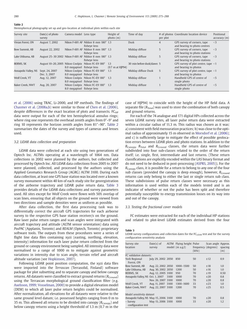
Table 3LiDAR survey configurations and collection dates for the FCLiDAR test and for the surveyconfiguration sensitivity analysis

Survey sitelocation

Date(s) ofsurvey

ALTMmodel

Flying height(m a.g.l)

Pulsefrequency(kHz)

Scan angle(degrees)

Approx.spacing(m)

FC validation datasets:York RegionalForest, ON

July 29, 2002 2050 850 50 ±12 0.9

Bow Summit, AB Aug. 22, 2002 2050 1000–1500 50 ±18 1.0Lake Utikuma, AB Aug. 30, 2002 2050 1200 50 ±16 1.0BERMS, SK Aug. 12, 2005 3100 950 70 ±19 0.50Annapolis Valley,NS Oct. 1, 2007 3100 1000 70 ±20 0.8

Nov. 26, 2007 3100 1000 70 ±20 0.8Wolf Creek, YT Aug. 11, 2007 3100 1300–1600 33 ±23 1.0Baker Creek, NWT Aug. 22, 2007 3100 1200 70 ±25 0.5

Model sensitivity datasetAnnapolis Valley,NS May 15, 2006 3100 1000 70 ±20 0.8– Surveyconfiguration test

May 15, 2006 3100 1000 33 ±20 1.2

Table 2Hemispherical photography set up and geo-location at individual plots within each site

Survey site Date(s) of photosurvey

Camera model Lens type Height ofphoto (m)

Time of day # of photosper plot

Coordinate location device Positionalaccuracy (m)

Vivian Forest, ON August 7, 2002 Nikon F-601 AF Nikkor 8 mm 180°fisheye lens

1.3 Dusk 4 GPS survey of corners, tapeand bearing to photo centres

b3

Bow Summit, AB August 22, 2002 Nikon F-601 AF Nikkor 8 mm 180°fisheye lens

1.3 Midday diffuse 5 GPS survey of corners, tapeand bearing to photo stations

b3

Lake Utikuma, AB August 25–30 2002 Nikon F-601 AF Nikkor 8 mm 180°fisheye lens

1.3 Midday diffuse 5 GPS survey of corners, tapeand bearing to photo stations

b3

BERMS, SK August 10–20, 2005 Nikon Coolpix8.0 megapixel

Nikon FC-E9 180°fisheye lens

1.3(0.7 m at HJP94)

30 min before dusk/dawn 5 GPS survey of plot centre, tapeand bearing to photos

b1

Annapolis Valley, NS Sept. 24, 2007Dec. 3, 2007

Nikon Coolpix8.0 megapixel


1.3 Midday diffuse Dusk 5 GPS survey of plot centre, tapeand bearing to photos

b1

Wolf Creek, YT Aug. 12, 2007 Nikon Coolpix8.0 megapixel


1.3 Midday diffuse 1 Handheld GPS of centre ofsingle photo

b5

Baker Creek, NWT Aug. 20, 2007 Nikon Coolpix8.0 megapixel


1.3 Midday diffuse 1 Handheld GPS of centre ofsingle photo

b5


et al. (2006) using TRAC, Li-2000, and HP methods. The findings ofChasmer et al. (2008a,b) were similar to those of Chen et al. (2006),despite differences in the exact location of plots and transects. FCHPdata were output for each of the ten hemispherical annulus rings;where ring one represents the overhead zenith angles from 0°–9° andring 10 represents the horizon zenith angles from 81°–90°. Table 2summarises the dates of the survey and types of cameras and lensesused.

3.2. LiDAR data collection and preparation

LiDAR data were collected at each site using two generations ofOptech Inc. ALTMs operating at a wavelength of 1064 nm. Datacollections in 2002 were planned by the authors, but collected andprocessed by Optech Inc. All LiDAR data collections from 2005 to 2007were planned, collected, and processed by the authors using theApplied Geomatics Research Group (AGRG) ALTM 3100. During eachdata collection, at least one GPS base stationwas located over a knownsurvey monument within 40 km of each study site for georegistrationof the airborne trajectory and LiDAR pulse return data. Table 3provides details of the LiDAR data collections and survey parametersused. All sites except for Wolf Creek were flown with 50% overlap ofscan lines, ensuring that all objects on the ground were viewed fromtwo directions and sample densities were as uniform as possible.

After data collection, the first data processing task was todifferentially correct the aircraft GPS trajectories for each airbornesurvey to the respective GPS base station receiver/s on the ground.Raw laser pulse return ranges and scan angles were integrated withaircraft trajectory and attitude (ALTM sensor orientation) data usingPosPAC (Applanix, Toronto) and REALM (Optech, Toronto) proprietarysoftware tools. The outputs from these procedures were a series offlight line data files containing xyzi (easting, northing, elevation,intensity) information for each laser pulse return collected from theground or canopy environment being sampled. All intensity data werenormalised to a range of 1000 m to mitigate against geometricvariations in intensity due to scan angle, terrain relief and aircraftaltitude variation (see Hopkinson, 2007).

Following LiDAR point position computation, the xyzi data fileswere imported into the Terrascan (Terrasolid, Finland) softwarepackage for plot subsetting and to separate canopy and below canopyreturns. All datasets were classified to extract ground returns (RGround)using the Terrascan morphological ground classification filter (e.g.Axelsson, 1999; Vosselman, 2000) to provide a digital elevation model(DEM) to which all laser pulse return heights could be normalised.After normalization, all elevations for all datasets were relative to thesame ground level datum; i.e. possessed heights ranging from 0 m to35 m. This allowed all returns to be divided into canopy (RCanopy) andbelow canopy returns using a height threshold of 1.3 m (0.7 m in the

case of HJP94) to coincide with the height of the HP field data. Aseparate file (RTotal) was used to store the combination of both canopyand ground returns.

For each of the 74 analogue and 171 digital HPs collected across theseven LiDAR survey sites, all laser pulse return data were extractedwithin a circular radius of 11.3 m. This radius was chosen as it was:a) consistent with fieldmensuration practices; b) was close to the opti-mal radius of approximately 15 m observed in Morsdorf et al. (2006);and c) is sufficiently large to mitigate the effect of possible geoloca-tion errors between LiDAR plots and photo stations. In addition to theRCanopy, RTotal and RGround classes, the return data were furthersubdivided into four sub-classes related to the order of the returnitself; i.e. single, first, intermediate and last returns. (These returnclassifications are explicitly encoded within the LAS binary format anddo not need to be deduced in post-processing (ASPRS, 2005)). For theRCanopy class, it is possible for a return to belong to any one of the foursub classes (provided the canopy is deep enough), however, RGroundreturns can only belong to either the last or single return sub class.These subdivisions of pulse return classes were necessary as thisinformation is used within each of the models tested and is anindicator of whether or not the pulse has been split and thereforepotentially susceptible to energy transmission losses on its way intoand out of the canopy.

3.3. Testing the fractional cover models

FC estimates were extracted for each of the individual HP stationsand related to plot-level LiDAR estimates derived from the four

Table 4Regression statistics of FCHP/FCLiDAR for each of the four models tested

Shaded cells denote best-fit lines that display: a) a slope within 5% of unity; b) an intercept within 5% of the origin; c) a coefficient of determination exceeding 0.75; i.e. N75%explanation of sample variance.


models described above Eqs. (2), (3), (4), and (6). The modelled FCLiDARestimates were compared with the FCHP observations for the first nineannulus rings (0°–81°) by starting with the first overhead ring (0°–9°)and sequentially adding the next ring until all nine had beencompared. Regression analyses were performed to assess thecorrespondence between LiDAR and HP estimates of FC. Followingthe comparison of the models over all 80 test plots, the models wereevaluated for their respective sensitivities to: i) variations in canopyheight; ii) variations in canopy structure/openness due to speciesclassification; iii) changes in LiDAR data acquisition settings.

In the case of i) and ii), this was possible by simply stratifying theresults from the 80 test plots into canopy height and structural class,re-evaluating the regression results and performing a residual analysisfor each model and each canopy class. To assess the sensitivity to dataacquisition settings it was necessary to perform a new analysis. It isknown that LiDAR survey configuration can have a marked influenceon canopy penetration (Chasmer et al., 2006; Hopkinson, 2007;Naesset 2004). To test whether or not a change in pulse repetitionfrequency (hence also pulse power and sampling density) would in-fluence FCLiDAR, two surveys were performed over a conifer plantation

Fig. 3. Regression results by forcing all FC data through the origin. Best fit slope represent

in the Annapolis Valley on the same day; the first at 70 kHz pulsefrequency, 3.7 kW peak pulse power, 0.8 m point spacing and thesecond at 33 kHz, 21.8 kW peak pulse power, 1.2 m point spacing.

4. Results and discussion

4.1. Testing the FCLiDAR models

The best-fit regression results comparing the 9 ring FCHP withFCLiDAR for the 80 independent test plots across all seven sites aresummarised in Table 4. It is observed that all three FCLiDAR models aresignificantly correlated (Pb0.01) with FCHP for all combinations of HPannulus rings from overhead zenith angles through to the average ofthe full hemisphere represented by rings 1–9. Generally, the FCLiDAR(IR)

model illustrates the best predictive capability of FCHP, with the ninecombinations of annulus rings displaying r2 values between 0.65 and0.78 This is followed by FCLiDAR(BL) with all ring combinations dis-playing r2 values between 0.61 and 0.75; then FCLiDAR(FR) with valuesbetween 0.58 to 0.75; and finally FCLiDAR(RR) with values between 0.57and 0.70. The best explanation of variance is found between FCLiDAR(IR)

ed by solid symbols and coefficient of determination represented by hollow symbols.

Fig. 5. Plot of mean residuals by canopy structure class and by FCLiDAR model. Error bars indicate 95% confidence limits on the mean residual.


and FCHP for annulus rings 1–4 (r2=0.78). However, while the best-fitline passes close to the origin, suggesting generally good predictivecapability throughout the range of values experienced, the FCLiDAR(IR)

model tends to over-estimate fractional cover with the slope neverexceeding 0.89 for the overhead annulus rings. In the case of theFCLiDAR(FR) model, the slope never exceeds 0.79 (rings 1–4) and theintercept approaches the origin only for the full hemisphere (rings 1–9) illustrating a tendency to over-estimate FC with weak predictivecapability for overhead zenith angles. For the FCLiDAR(RR) model, theoverall explanation of variance and intercept values do not deviatesignificantly from those of FCLiDAR(FR), however, the magnitude of theslope is always within 10% (i.e. close to unity) suggesting that thevalues predicted are closer in magnitude to actual FCHP values. Of thefour models tested, only FCLiDAR(BL) demonstrates a combination ofhigh explanation of variance, a slope near to unity with an interceptnear the origin; i.e. the FCLiDAR(BL) model demonstrates good predictivecapability across the full range of values requiring no calibration.

By forcing all data through the origin (as it is impossible to have anegative FC) we see in Fig. 3, that the intensity-based FCLiDAR models(IR and BL) tend towards better predictive capability for overheadzenith angles, while the pulse return ratio models (FR and RR) tendtoward a better characterisation of the entire hemisphere. Further,while FCLiDAR(FR), FCLiDAR(RR) and FCLiDAR(IR) tend to over-estimate FCHPfor almost all zenith angles, we see that FCLiDAR(BL) demonstrates anear 1:1 predictive capability within the 5° to 20° range of meanzenith angles with optimal results for HP rings 1–3. These annulusrings are representative of overhead canopy conditions and representzenith angles that are similar to the range of scan angles emitted intypical airborne LiDAR surveys.

The results displayed in Table 4 and Fig. 3 are consistent with thefindings from the original intensity-based model developmentpresented in Hopkinson and Chasmer (2007), however, the explana-tion of variance is up to 15% weaker for all models. One over-ridingfactor leading to these weaker regression results is that the datasetsused in the original model development were collected over a rela-tively uniform canopy class (mixed wood and hardwood), using anequivalent survey configuration throughout. In the test dataset, the

Fig. 4. Regression plots of FCHP^against FCLiDAR models for each canopy structural class. Colou

the canopy classes. The thick black line represents all data.

vegetation species (Table 1), canopy attributes (Fig. 2) and surveyconfigurations (Table 3) are highly variable and so an increased level ofuncertainty or loss of predictive capability is to be expected. Some ofthe systematic factors that may influence the efficacy of each of themodels are discussed below.

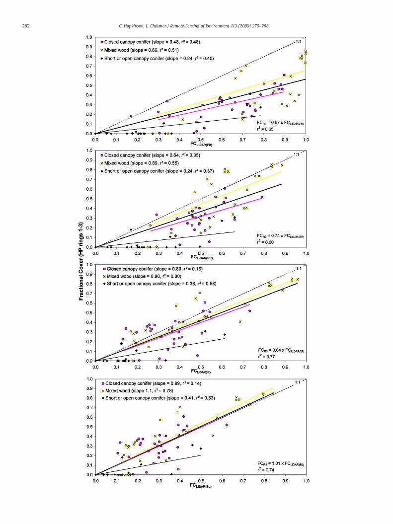
4.2. The influence of canopy structure

In an attempt to represent overhead canopy conditions only, theremainder of the analysis compares FCLiDAR to FCHP for annulus rings1–3. The improvement in FCLiDAR model capability from the returnratio models (RR and FR) to the intensity ratio (IR) to the Beer's Lawmodified intensity ratio (BL) is observed in Fig. 4. Further, whenstratified by canopy structural class, each of the four models dem-onstrates different behaviour. For all FCLiDAR models, the mixed wood/hardwood canopy class consistently displays the best results (r2=0.51to 0.80). For both conifer canopy classes, the regression results aregenerally weak for all four FCLiDAR models (r2=0.14 to 0.58). Fur-thermore, the nature of the FCLiDAR model error differs, with the closedcanopy conifer class tending towards a slight over-estimation in theFR, RR and IR models, with the open and short canopy conifer classtending toward a consistent and large over-estimate of FCHP for all fourmodels (Fig. 4).

The improvement in the magnitude of predictive capability fromthe FCLiDAR(FR) to FCLiDAR(RR) to FCLiDAR(IR) to FCLiDAR(BL) models is mostclearly illustrated by plotting the magnitudes of the mean residuals. InFig. 5 we observe that the mean overestimate in FCLiDAR(FR) for all datais 30%, for FCLiDAR(RR) it is 16%, for FCLiDAR(IR) it is 6%, while there is asmall but not significant (p=0.05) overestimate of b1% for FCLiDAR(BL).While the mean residuals for all canopy classes are positive for the FR,RR and IR models, the opposed behaviour of the three canopy classesis clear in the BL model. Therefore, by including these three conifercanopy classes in the analysis they have effectively compensated oneanother. This is important to note because it demonstrates that whilethe FCLiDAR(BL) model results are generally superior to the other threemodels when applied across a broad range of canopy classes, it may beprone to bias if applied exclusively to any distinct forest canopy class.

red lines represent the best fit regression line that passes through the origin for each of

Original_text: �

Original_text: �

Original_text: �

Original_text: �

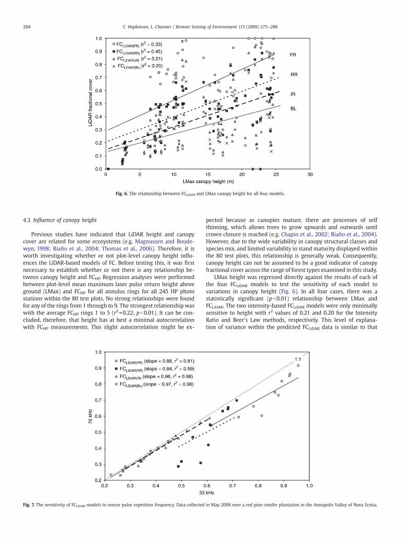
Fig. 6. The relationship between FCLiDAR and LMax canopy height for all four models.


4.3. Influence of canopy height

Previous studies have indicated that LiDAR height and canopycover are related for some ecosystems (e.g. Magnussen and Boude-wyn, 1998; Riaño et al., 2004; Thomas et al., 2006). Therefore, it isworth investigating whether or not plot-level canopy height influ-ences the LiDAR-based models of FC. Before testing this, it was firstnecessary to establish whether or not there is any relationship be-tween canopy height and FCHP. Regression analyses were performedbetween plot-level mean maximum laser pulse return height aboveground (LMax) and FCHP for all annulus rings for all 245 HP photostations within the 80 test plots. No strong relationships were foundfor any of the rings from 1 through to 9. The strongest relationshipwaswith the average FCHP rings 1 to 5 (r2=0.22, pb0.01). It can be con-cluded, therefore, that height has at best a minimal autocorrelationwith FCHP measurements. This slight autocorrelation might be ex-

Fig. 7. The sensitivity of FCLiDAR models to sensor pulse repetition frequency. Data collected

pected because as canopies mature, there are processes of selfthinning, which allows trees to grow upwards and outwards untilcrown closure is reached (e.g. Chapin et al., 2002; Riaño et al., 2004).However, due to the wide variability in canopy structural classes andspecies mix, and limited variability in standmaturity displayed withinthe 80 test plots, this relationship is generally weak. Consequently,canopy height can not be assumed to be a good indicator of canopyfractional cover across the range of forest types examined in this study.

LMax height was regressed directly against the results of each ofthe four FCLiDAR models to test the sensitivity of each model tovariations in canopy height (Fig. 6). In all four cases, there was astatistically significant (pb0.01) relationship between LMax andFCLiDAR. The two intensity-based FCLiDAR models were only minimallysensitive to height with r2 values of 0.21 and 0.20 for the IntensityRatio and Beer's Law methods, respectively. This level of explana-tion of variance within the predicted FCLiDAR data is similar to that

in May 2006 over a red pine conifer plantation in the Annapolis Valley of Nova Scotia.


observed between LMax and the actual FCHP values (max r2=0.22).This similarity suggests that the intensity-based methods have asimilar level of sensitivity to canopy height as exists in reality. Con-versely, the pulse return ratio methods demonstrate increased sen-sitivity to variations in height, (with an r2 values of 0.33 (FR) and 0.45(RR)), which suggest that the incorporation of a height term mightpotentially improve these models. This enhanced sensitivity is likelydue to the reduced probability of obtaining ground level returns in tallcanopies; i.e. more returns are ‘trapped’ in taller canopies than shortercanopies. The intensity-based methods are less sensitive to height inthis way because the differences in probability associated with tallerand shorter canopies are essentially directly accounted for by thevariations observed in the recorded intensity.

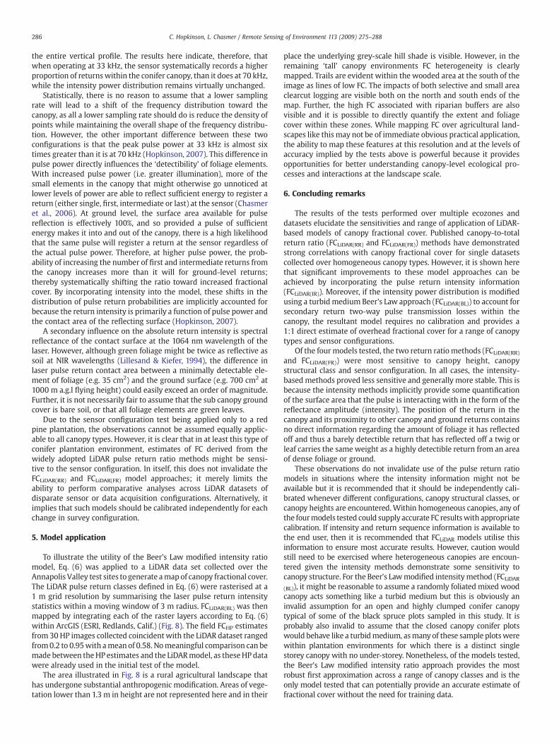
4.4. Influence of sensor configuration

The comparative FCLiDAR results obtained from the 33 kHz and70 kHz sensor pulse frequency configurations for 10 plots within a redpine plantation are illustrated in Fig. 7. By comparing the samplemeans, it was found that the difference in pulse power and samplingdensity associated with these two configurations produced signifi-

Fig. 8. A 1 m grid resolution image of FCLiDAR(BL) at the scale of individual canopy elements emixed wood landscape in the Annapolis Valley of Nova Scotia during August of 2006.

cantly different results for FCLiDAR(RR) (mean difference=0.11, p=0.07)and FCLiDAR(FR) (mean difference=0.08, p=0.10), while there is nosignificant difference for either of the intensity-based methods (p=0.72 for FCLiDAR(IR) and p=0.81 for FCLiDAR(BL)). The regression plot inFig. 7 illustrates that both intensity-based FCLiDAR models are almostcompletely insensitive to pulse frequency. Meanwhile, both returnratio models (FR and RR) illustrate a tendency toward comparativelyhigher estimates of FC at the lower frequency or higher pulse powerconfiguration of 33 kHz. Further the increased scatter in the FR and RRmodel observations in Fig. 7 implies that there is random behaviourinherent in the return ratio approaches that is mitigated by theinclusion of intensity data. This also suggests that one of the likelyreasons for reduced coefficient of determination results in Table 4 andFig. 3 for ‘all data’ in the FCLiDAR(RR) and FCLiDAR(FR) models are due tothe variability of sensors and survey configurations used (Table 3).

The return ratio models demonstrate increased sensitivity to pulserepetition frequency due to the difference in the information contentbetween a pulse return frequency distribution and an intensity powerdistribution. The ratio of canopy-to-total returns (models (2) and (3))provides a direct quantification of the frequency of points that werereflected from the canopy vs. the total frequency of points reflected in

xceeding 1.3 m in height. Map illustrates a combined agricultural and forested Acadian


the entire vertical profile. The results here indicate, therefore, thatwhen operating at 33 kHz, the sensor systematically records a higherproportion of returnswithin the conifer canopy, than it does at 70 kHz,while the intensity power distribution remains virtually unchanged.

Statistically, there is no reason to assume that a lower samplingrate will lead to a shift of the frequency distribution toward thecanopy, as all a lower sampling rate should do is reduce the density ofpoints while maintaining the overall shape of the frequency distribu-tion. However, the other important difference between these twoconfigurations is that the peak pulse power at 33 kHz is almost sixtimes greater than it is at 70 kHz (Hopkinson, 2007). This difference inpulse power directly influences the ‘detectibility’ of foliage elements.With increased pulse power (i.e. greater illumination), more of thesmall elements in the canopy that might otherwise go unnoticed atlower levels of power are able to reflect sufficient energy to register areturn (either single, first, intermediate or last) at the sensor (Chasmeret al., 2006). At ground level, the surface area available for pulsereflection is effectively 100%, and so provided a pulse of sufficientenergy makes it into and out of the canopy, there is a high likelihoodthat the same pulse will register a return at the sensor regardless ofthe actual pulse power. Therefore, at higher pulse power, the prob-ability of increasing the number of first and intermediate returns fromthe canopy increases more than it will for ground-level returns;thereby systematically shifting the ratio toward increased fractionalcover. By incorporating intensity into the model, these shifts in thedistribution of pulse return probabilities are implicitly accounted forbecause the return intensity is primarily a function of pulse power andthe contact area of the reflecting surface (Hopkinson, 2007).

A secondary influence on the absolute return intensity is spectralreflectance of the contact surface at the 1064 nm wavelength of thelaser. However, although green foliage might be twice as reflective assoil at NIR wavelengths (Lillesand & Kiefer, 1994), the difference inlaser pulse return contact area between a minimally detectable ele-ment of foliage (e.g. 35 cm2) and the ground surface (e.g. 700 cm2 at1000 m a.g.l flying height) could easily exceed an order of magnitude.Further, it is not necessarily fair to assume that the sub canopy groundcover is bare soil, or that all foliage elements are green leaves.

Due to the sensor configuration test being applied only to a redpine plantation, the observations cannot be assumed equally applic-able to all canopy types. However, it is clear that in at least this type ofconifer plantation environment, estimates of FC derived from thewidely adopted LiDAR pulse return ratio methods might be sensi-tive to the sensor configuration. In itself, this does not invalidate theFCLiDAR(RR) and FCLiDAR(FR) model approaches; it merely limits theability to perform comparative analyses across LiDAR datasets ofdisparate sensor or data acquisition configurations. Alternatively, itimplies that such models should be calibrated independently for eachchange in survey configuration.

5. Model application

To illustrate the utility of the Beer's Law modified intensity ratiomodel, Eq. (6) was applied to a LiDAR data set collected over theAnnapolis Valley test sites to generate amap of canopy fractional cover.The LiDAR pulse return classes defined in Eq. (6) were rasterised at a1 m grid resolution by summarising the laser pulse return intensitystatistics within a moving window of 3 m radius. FCLiDAR(BL) was thenmapped by integrating each of the raster layers according to Eq. (6)within ArcGIS (ESRI, Redlands, Calif.) (Fig. 8). The field FCHP estimatesfrom 30 HP images collected coincident with the LiDAR dataset rangedfrom0.2 to 0.95with amean of 0.58. Nomeaningful comparison can bemade between theHP estimates and the LiDARmodel, as theseHP datawere already used in the initial test of the model.

The area illustrated in Fig. 8 is a rural agricultural landscape thathas undergone substantial anthropogenic modification. Areas of vege-tation lower than 1.3 m in height are not represented here and in their

place the underlying grey-scale hill shade is visible. However, in theremaining ‘tall’ canopy environments FC heterogeneity is clearlymapped. Trails are evident within the wooded area at the south of theimage as lines of low FC. The impacts of both selective and small areaclearcut logging are visible both on the north and south ends of themap. Further, the high FC associated with riparian buffers are alsovisible and it is possible to directly quantify the extent and foliagecover within these zones. While mapping FC over agricultural land-scapes like this may not be of immediate obvious practical application,the ability to map these features at this resolution and at the levels ofaccuracy implied by the tests above is powerful because it providesopportunities for better understanding canopy-level ecological pro-cesses and interactions at the landscape scale.

6. Concluding remarks

The results of the tests performed over multiple ecozones anddatasets elucidate the sensitivities and range of application of LiDAR-based models of canopy fractional cover. Published canopy-to-totalreturn ratio (FCLiDAR(RR) and FCLiDAR(FR)) methods have demonstratedstrong correlations with canopy fractional cover for single datasetscollected over homogeneous canopy types. However, it is shown herethat significant improvements to these model approaches can beachieved by incorporating the pulse return intensity information(FCLiDAR(IR)). Moreover, if the intensity power distribution is modifiedusing a turbidmedium Beer's Law approach (FCLiDAR(BL)) to account forsecondary return two-way pulse transmission losses within thecanopy, the resultant model requires no calibration and provides a1:1 direct estimate of overhead fractional cover for a range of canopytypes and sensor configurations.

Of the fourmodels tested, the two return ratio methods (FCLiDAR(RR)

and FCLiDAR(FR)) were most sensitive to canopy height, canopystructural class and sensor configuration. In all cases, the intensity-based methods proved less sensitive and generally more stable. This isbecause the intensity methods implicitly provide some quantificationof the surface area that the pulse is interacting with in the form of thereflectance amplitude (intensity). The position of the return in thecanopy and its proximity to other canopy and ground returns containsno direct information regarding the amount of foliage it has reflectedoff and thus a barely detectible return that has reflected off a twig orleaf carries the same weight as a highly detectible return from an areaof dense foliage or ground.

These observations do not invalidate use of the pulse return ratiomodels in situations where the intensity information might not beavailable but it is recommended that it should be independently cali-brated whenever different configurations, canopy structural classes, orcanopy heights are encountered.Within homogeneous canopies, any ofthe fourmodels tested could supplyaccurate FC resultswith appropriatecalibration. If intensity and return sequence information is available tothe end user, then it is recommended that FCLiDAR models utilise thisinformation to ensure most accurate results. However, caution wouldstill need to be exercised where heterogeneous canopies are encoun-tered given the intensity methods demonstrate some sensitivity tocanopy structure. For the Beer's Lawmodified intensitymethod (FCLiDAR(BL)), it might be reasonable to assume a randomly foliated mixed woodcanopy acts something like a turbid medium but this is obviously aninvalid assumption for an open and highly clumped conifer canopytypical of some of the black spruce plots sampled in this study. It isprobably also invalid to assume that the closed canopy conifer plotswould behave like a turbidmedium, asmany of these sample plotswerewithin plantation environments for which there is a distinct singlestorey canopy with no under-storey. Nonetheless, of the models tested,the Beer's Law modified intensity ratio approach provides the mostrobust first approximation across a range of canopy classes and is theonly model tested that can potentially provide an accurate estimate offractional cover without the need for training data.


Acknowledgements

Dr. Chris Hopkinson acknowledges infrastructure funding from theCanada Foundation for Innovation (CFI) and partial funding supportfrom NSERC under the College and Community Innovation Program.Dr. Laura Chasmer acknowledges NSERC PGSB and OGSST post-graduate scholarship support. Optech Incorporated and the CanadianConsortium for LiDAR Environmental Applications Research (C-CLEAR)are acknowledged for assisting with the provision of the LiDARdatasets. Many students and colleagues are gratefully acknowledgedfor their assistance with the collection of field data.

References

ASPRS (2005). LAS specification version 1.1 March 07, 2005.Data format documentationcreated by the LiDAR sub-committee of the American Society of Photogrammetryand Remote Sensing Available online: http://www.asprs.org/society/committees/lidar/lidar_downloads.html 11 pp. Last accessed on July 1st, 2008.

Axelsson, P. (1999). Processing of laser scanner data algorithms and applications. ISPRSJournal of Photogrammetry and Remote Sensing, 54, 138−147.

Barilotti, A., Turco, S., & Alberti, G. (2006). LAI determination in forestry ecosystems byLiDAR data analysis. Workshop on 3D Remote Sensing in Forestry, 14–15/02/2006,BOKU Vienna.

Barr, A. G., Griffis, T. J., Black, T. A., Lee, X., Staebler, R. M., Fuentes, J. D., et al. (2002).Comparing the carbon balances of boreal and temperate deciduous forest stands.Canadian Journal of Forest Research, 32, 813−822.

Chasmer, L., Barr, A., Hopkinson, C., McCaughey, H., Treitz, P., & Black, A. (2009). Scalingand assessment of GPP from MODIS using a combination of airborne LiDARand eddy covariance measurements over jack pine forests. Remote Sensing ofEnvironment, 113, 82−93.

Chasmer, L., Hopkinson, C., Smith, B., & Treitz, P. (2006). Examining the influence ofchanging laser pulse repetition frequencies on conifer forest canopy returns. Pho-togrammetric Engineering and Remote Sensing, 17(12), 1359−1367.

Chasmer, L., McCaughey, H., Barr, A., Black, A., Shashkov, A., Treitz, P., et al. (2008a).Investigating light use efficiency (LUE) across a jack pine chronosequence duringdry and wet years. Tree Physiology, 28, 1395−1406.

Chasmer, L., Hopkinson, C., Treitz, P., McCaughey, H., Barr, A., & Black, A. A. (2008b). Alidarbased hierarchical approach to assessing MODIS fPAR. Remote Sensing ofEnvironment, 112, 4344−4357.

Chasmer, L., Kljun, N., Barr, A., Black, A., Hopkinson, C., & McCaughey, H. (in press).Vegetation structural and elevation influences on CO2 uptake within a mature jackpine forest in Saskatchewan, Canada. Canadian Journal of Forest Research.

Chapin, F. S., III, Matson, P. A., & Mooney, H. A. (2002). Principles of Terrestrial EcosystemEcology.New York: Springer–Verlag Inc. 436 pp.

Chen, J. M. (1996). Optically-based methods for measuring seasonal variation in leaf areaindex of boreal conifer forests. Agricultural and Forest Meteorology, 80, 135−163.

Chen, J. M., Chen, X., Ju, W., & Geng, X. (2005). A remote sensing-driven distributedhydrological model: Mapping evapotranspiration in a forested watershed. Journalof Hydrology, 305, 15−39.

Chen, B., Chen, J. M., Mo, G., Yuan, K., Higuchi, K., & Chan, D. (2007). Modeling andscaling coupled energy, water, and carbon fluxes based on remote sensing: Anapplication to Canada's landmass. Journal of Hydrometeorology, 8, 123−143.

Chen, J. M., Govind, A., Sonnentag, O., Zhang, Y., Barr, A., & Amiro, B. (2006). Leaf areaindex measurements at Fluxnet-Canada forest sites. Agricultural and ForestMeteorology, 140, 257−268.

Fernandes, R. A., Miller, J. R., Chen, J. M., & Rubinstein, I. G. (2004). Evaluating imagebased estimates of leaf area index in boreal conifer stands over a range of scalesusing high-resolution CASI imagery. Remote Sensing of Environment, 89, 200−216.

Gower, S. T., Kucharik, C. J., & Norman, J. M. (1999). Direct and indirect estimation of leafarea index, fAPAR, and net primary production of terrestrial ecosystems. RemoteSensing of Environment, 70, 29−51.

Hall, F. G., Botkin, D. B., Strebel, D. E.,Woods, K. D., & Goetz, S. J. (1991). Large scale patternsof forest succession as determined by remote sensing. Ecology, 72(2), 628−640.

Heinsch, F.A., Reeves, M., Bowker, C.F., Votava, P., Kang, S., Milesi, C. et al., 2003. User'sGuide, GPP and NPP (MOD17A2/A3, NASA MODIS Land Algorithm, Version 1.2.www.ntsg.umt.edu/modis/MOD17UsersGuide.pdf

Heinsch, F. A., Zhao, M., Running, S. W., Kimball, J. S., Nemani, R. R., Davis, K. J., et al.(2006). Evaluation of remote sensing based terrestrial productivity from MODISusing regional tower eddy flux network observations. IEEE Transactions onGeoscience and Remote Sensing, 44(7), 1908−1925.

Hopkinson, C. (2007). The influence of flying altitude and beam divergence on canopypenetration and laser pulse return distribution characteristics. Canadian Journal ofRemote Sensing, 33(4), 312−324.

Hopkinson, C., & Chasmer, L. E. (2007). Using discrete laser pulse return intensity tomodel canopy transmittance. The Photogrammetric Journal of Finland, 20(2), 16−26.

Hopkinson, C., & Demuth, M. D. (2006). Using airborne LiDAR to assess the influence ofglacier downwasting to water resources in the Canadian Rocky Mountains. Cana-dian Journal of Remote Sensing, 32(2), 212−222.

Hopkinson, C., Chasmer, L. E., & Hall, R. J. (2008). The uncertainty in conifer plantationgrowth prediction from multitemporal LiDAR datasets. Remote Sensing of Environ-ment, 112(3), 1168−1180.

Hopkinson, C., Chasmer, L. E., Lim, K., Treitz, P., & Creed, I. (2006). Towards a universalLiDAR canopy height indicator. Canadian Journal of Remote Sensing, 32(2), 139−153.

Hopkinson, C., Chasmer, L. E., Zsigovics, G., Creed, I., Sitar, M., Kalbfleisch, W., et al.(2005). Vegetation class dependent errors in LiDAR ground elevation and canopyheight estimates in a Boreal wetland environment. Canadian Journal of RemoteSensing, 31(2), 191−206.

Hopkinson, C., Sitar, M., Chasmer, L. E., & Treitz, P. (2004). Mapping snowpack depthbeneath forest canopies using airborne LiDAR. Photogrammetric Engineering andRemote Sensing, 70(3), 323−330.

Kotchenova, S., Shabanov, N., Knyazikhin, Y., Davis, A., Dubayah, R., & Myneni, R. (2003).Modeling LiDAR waveforms with time-dependent stochastic radiative transfertheory for estimations of forest structure.Journal of Geophysical Research, 108(D15),4484. doi:10.1029/2002JD003288, 2003.

Kotchenova, S., Song, X., Shabanov, N., Potter, C., Knyazikhin, Y., & Myneni, R. (2004).LiDAR remote sensing for modeling gross primary production of deciduous forests.Remote Sensing of Environment, 92, 158−172.

Kusakabe, T., Tsuzuki, H., Hughes, G., & Sweda, T. (2000). Extensive forest leaf areasurvey aiming at detection of vegetation change in subarctic-boreal zone. PolarBioscience, 13, 133−146.

Law, B. E., Falge, E., Gu, L., Baldocchi, D., Bakwin, P., Berbigier, P., et al. (2002).Environmental controls over carbon dioxide and water vapor exchange of ter-restrial vegetation. Agricultural and Forest Meteorology, 113, 97−120.

Leblanc, S. G., Chen, J. M., Fernandes, R., Deering, D., & Conley, A. (2005). Methodologycomparison for canopy structure parameters extraction from digital hemisphericalphotography in boreal forests. Agricultural and Forest Meteorology, 129, 187−207.

Lefsky, M. A., Cohen, W. B., Acker, S. A., Parker, G. G., Spies, T. A., & Harding, D. (1999).LiDAR remote sensing of the canopy structure and biophysical properties ofDouglas-fir Western hemlock forests. Remote Sensing of Environment, 70, 339−361.

Lefsky, M. A., Turner, D., Guzy, M., & Cohen, W. (2005). Combining LIDAR estimates ofaboveground biomass and Landsat estimates of stand age for spatially extensivevalidation of modeled forest productivity. Remote Sensing of Environment, 95,549−558.

Leuning, R., Cleugh, H. A., Zegelin, S. J., & Hughes, D. (2005). Carbon and water fluxesover a temperate Eucalyptus forest and a tropical wet/dry savannah in Australia:measurements and comparison with MODIS remote sensing estimates. Agriculturaland Forest Meteorology, 129, 151−173.

Lillesand, T. M., & Kiefer, R. W. (1994). Remote Sensing and Photo Interpretation, 3rd. ed.New York: John Wiley & Sons 750 pp.

Lovell, J., Jupp, D., Culvenor, D., & Coops, N. (2003). Using airborne and groundbasedranging LiDAR to measure canopy structure in Australian forests. Canadian Journalof Remote Sensing, 29(5), 607−622.

Magnussen, S., & Boudewyn, P. (1998). Derivations of stand heights from airborne laserscanner data with canopy-based quantile estimators. Canadian Journal of ForestResearch, 28, 1016−1031.

Morsdorf, F., Kotz, B., Meier, E., Itten, K. I., & Allgower, B. (2006). Estimation of LAI andfractional cover from small footprint airborne laser scanning data based on gapfraction. Remote Sensing of Environment, 104(1), 50−61.

Naesset, E. (2004). Effects of different flying altitudes on biophysical stand propertiesestimated from canopy height and density measured with a small-footprintairborne scanning laser. Remote Sensing of Environment, 91, 243−255.

Nelson, R., Krabill, W., & Maclean, G. (1984). Determining forest canopy characteristicsusing airborne laser data. Remote Sensing of Environment, 15, 201−212.

Parker, G. G., Lefsky, M. A., & Harding, D. J. (2001). Light transmittance in forest canopiesdetermined using airborne laser altimetry and in-canopy quantum measurements.Remote Sensing of Environment, 76, 298−309.

Pomeroy, J. W., & Dion, K. (1996). Winter radiation extinction and reflection in a borealpine canopy: measurements and modelling. Hydrological Processes, 10, 1591−1608.

Pomeroy, J. W., Granger, R. J., Hedstrom, N. R., Gray, D. M., Elliott, J., Pietroniro, A., &Janowicz, J. R. (2005). The process hydrology approach to improving prediction ofungauged basins in Canada. In C. Spence, J. Pomeroy, & A. Pietroniro (Eds.), Pre-dictions in Ungauged Basins: Approaches for Canada’s Cold Regions. Canada: CanadianSociety for Hydrological Sciences, Environment pp. 67–100.

Popescu, S., Wynne, R., & Nelson, R. (2003). Measuring individual tree crown diameterswith LiDAR and assessing its influence on estimating forest volume and biomass.Canadian Journal of Remote Sensing, 29(5), 564−577.

Quinton, W. L., Shirazi, T., Carey, S. K., & Pomeroy, J. W. (2005). Soil water storage andactive-layer development in a sub-alpine tundra hillslope, southern YukonTerritory, Canada. Permafrost and Periglacial Processes, 16, 369−382.

Riaño, D., Valladares, F., Condes, S., & Chuvieco, E. (2004). Estimation of leaf area indexand covered ground from airborne laser scanner (LiDAR) in two contrasting forests.Agricultural and Forest Meteorology, 124(3–4), 269−275.

Running, S.W.,Nemani, R. R., Heinsch, F. A., Zhao,M., Reeves,M. C., &Hashimoto,H. (2004).A continuous satellite-derived measure of global terrestrial primary production.BioScience, 54, 547−560.

Schwalm, C. R., Black, T. A., Amiro, B. D., Arain, M. A., Barr, A. G., & Bourque, C. P. A. (2006).Photosynthetic light use efficiency of three biomes across an east-west continental-scale transect in Canada. Agricultural and Forest Meteorology, 140, 269−286.

Solberg, S., Næsset, E., Hanssen, K. H., & Christiansen, E. (2006). Mapping defoliationduring a severe insect attack on Scots pine using airborne laser scanning. RemoteSensing of Environment, 102, 364−376.

Thomas, V., Treitz, P., McCaughey, J. H., &Morrison, I. (2006). Mapping stand-level forestbiophysical variables for a mixedwood boreal forest using LiDAR: An examination ofscanning density. Canadian Journal of Forest Research, 36(1), 34−47.

Tian, Y., Wang, Y., Zhang, Y., Knyazikhin, Y., Bogaert, J., & Myneni, R. (2002). Radiativetransfer based scaling of LAI retrievals from reflectance data of different resolutions.Remote Sensing of Environment, 84, 143−159.

http://www.asprs.org/society/committees/lidar/lidar_downloads.html

http://www.asprs.org/society/committees/lidar/lidar_downloads.html

http://www.ntsg.umt.edu/modis/MOD17UsersGuide.pdf

http://dx.doi.org/10.1029/2002JD003288


Tucker, C. J., Fung, I. Y., Keeling, C. D., & Gammon, R. H. (1986). Relationship between CO2

variation and a satellite-derived vegetation index. Nature, 319, 195−199.Todd, K. W., Csillag, F., & Atkinson, P. M. (2003). Three-dimensional mapping of light

transmittance and foliage distribution using LiDAR. Canadian Journal of RemoteSensing, 29(5), 544−555.

Vosselman, G. (2000). Slope based filtering of laser altimetry data, Vol. XXXIII. (pp. 935−942)Amsterdam, The Netherlands: ISPRS Part B3.

Zhang, Y., Chen, J., & Miller, J. (2005). Determining digital hemispherical photographexposure for leaf area index estimation. Agricultural and Forest Meteorology, 133,166−181.

testing lidar models of fractional cover across multiple...

Documents