Precision LiDAR Mapping of Transportation Corridors Using LiDAR-Specific Ground Targets

Nora Csanyi

Department of Civil and Environmental Engineering and Geodetic Science The Ohio State University, 1216 Kinnear Rd, Columbus, Ohio 43212

Phone: 614-378-3567 Fax: 614-292-8062

e-mail: nora@cfm.ohio-state.edu

Abstract Transportation corridor mapping to support engineering planning and change detection of the road network requires high spatial resolution and extremely high, engineering scale mapping accuracy. With the recent advances of LiDAR technology, the accuracy potential of LiDAR data has significantly improved. State-of-the-art LiDAR systems can provide pulse repetition rate of up to 100 kHz, and range measurement accuracy at 2-3 cm level, which in theory, could support engineering scale mapping. However, due to the complexity of LiDAR systems, the various components as well as their spatial relationship can introduce errors that can degrade LiDAR data accuracy, and even after rigorous system calibration, some errors can still be present in the data. These errors are typically dominated by navigation errors and cannot be totally eliminated without introducing absolute control information into the LiDAR data. Therefore, to support applications that require extremely high, engineering scale mapping accuracy, such as transportation corridor mapping, this paper proposes the use of LiDAR-specific ground control targets. To determine the optimal LiDAR target design, simulation were carried out, and based on the simulations targets were fabricated. This paper provides a description of the optimal LiDAR target design, as well as a detailed performance analysis, investigating the achievable LiDAR data accuracy improvement using the LiDAR-specific ground control targets. Test results, based on two test flights using the Optech ALTM 30/70 LiDAR system operated by the Ohio Department of Transportation have shown that using the LiDAR-specific targets, transportation corridor mapping accuracy can be improved to cm-level. 1. Introduction

The deployment of LiDAR (Light Detection and Ranging) systems has recently experienced enormous growth. Efficiency and affordability have made LiDAR a primary tool for collecting a variety of high quality surface data in much shorter periods of time than previously possible. In addition, LiDAR technology has seen enormous developments in recent years, in particular the pulse rate frequency increased significantly; while earlier systems provided 33 kHz pulse rate, state-of-the-art LiDAR systems are capable of providing pulse repetition rate of up to 100 kHz. Furthermore, the ranging accuracy improved to 2-3 cm level, and the availability of intensity signal became common (Toth, 2004). These developments resulted in improved data quality in terms of higher point density and better accuracy, which in turn, opened new application areas of LiDAR (Renslow, 2005). Modern LiDAR systems with the cm-level ranging accuracy and high pulse rate, in theory, could support engineering scale mapping, like precise mapping of transportation corridors to support engineering planning and change detection of the road network. However, besides the laser ranging error there are several potential error sources that can degrade the accuracy of the acquired LiDAR data.

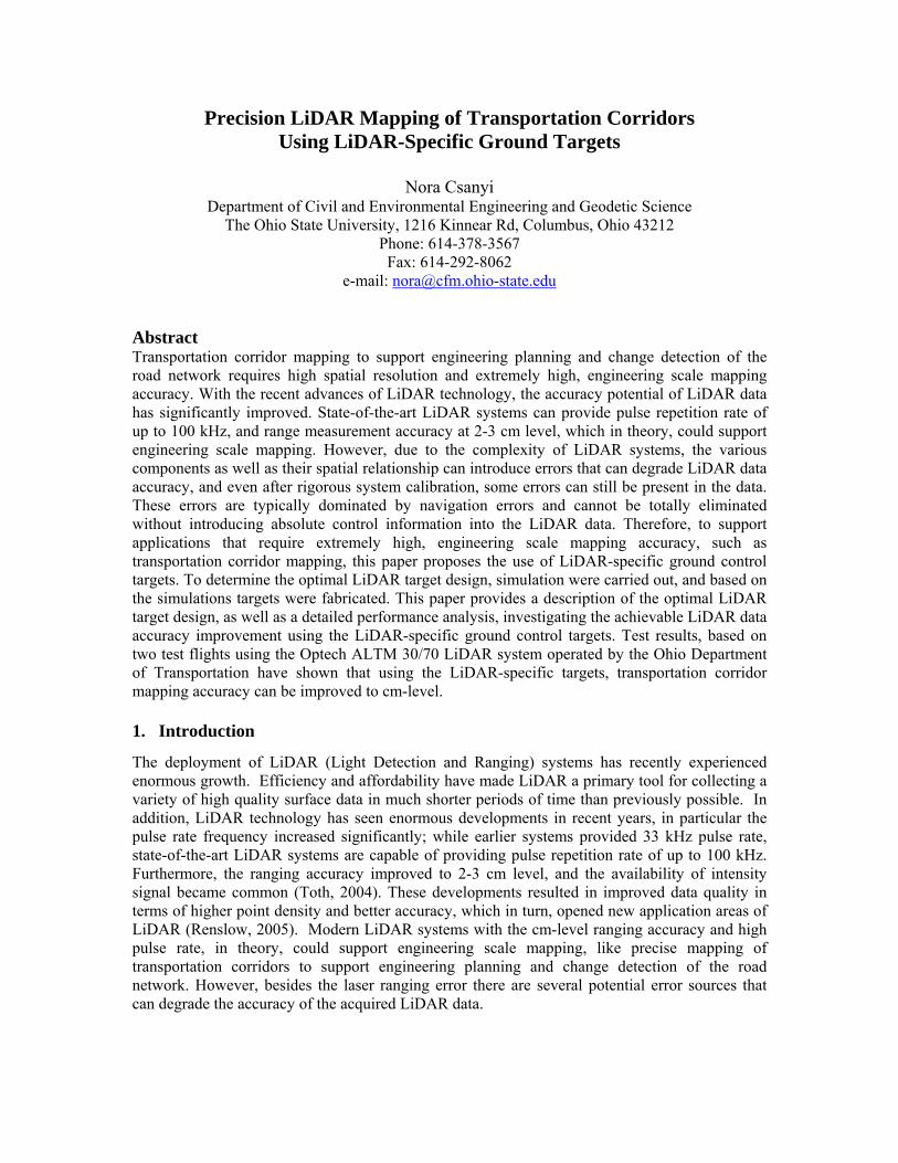
LiDAR systems are complex multi-sensor systems, and incorporate at least three main sensors; the GPS and INS navigation sensors, and the laser-scanning device (see Figure 1.). The laser system measures the distance from the sensor to the ground surface. The coordinates of the ground point from where the laser pulse returned can be calculated if the travel distance of the laser pulse, the laser beam orientation, and the position of the laser scanner are known. Due to the high complexity of the system, a number of potential error sources can degrade the accuracy of the acquired data. Errors in laser scanning data can result from sensor platform position and attitude errors (or errors in the navigation), individual sensor calibration or measurement errors, and inter-sensor calibration errors (or a misalignment between the different sensors). Any of the above error sources translates to an error in the calculated coordinates of the measured LiDAR points (see Figure 1.). Baltsavias (1999) presents an overview of basic relations and error formulae concerning airborne laser scanning and a large number of publications report the existence of systematic errors. Even after rigorous system calibration errors can be present in the data, and usually navigation errors dominate. The errors become evident as discrepancies between overlapping strips and at ground control surfaces.

Figure 1. LiDAR system components, and an example LiDAR point cloud

collected over a transportation corridor

In the last few years many strip adjustment methods have been developed to eliminate the discrepancies between overlapping strips, and thereby improve the LiDAR data accuracy (Burman, 2002; Filin, 2003; Toth et al., 2002). Most of the strip adjustment methods only require relative control information (tie points between overlapping strips) with absolute control information being optional. However, for applications requiring cm-level, engineering scale mapping accuracy, absolute control information is essential, since eliminating the relative discrepancies between overlapping strips does not provide an absolute check of the dataset. The usually applied control information in LiDAR data is horizontal planes with known elevations, or measuring control profiles across the strips. The problem with these types of control information is that they only provide vertical control. However, horizontal errors in LiDAR data are usually more significant (Vosselman and Maas, 2001.) than vertical errors. Therefore, to achieve the demanding accuracy required by engineering scale mapping, such as transportation corridor mapping, 3-dimensional ground control information in the form of well identifiable LiDAR-specific ground control targets are necessary. These ground control targets can then be used in the strip adjustment process or after strip adjustment to correct the remaining absolute errors in the corrected strips.

ZIN

ZL

XIN

XLYL

YIN

ZM

XM

YM

rM,k

rM,IN

k∆Z

∆X∆Y

rL

k

GPS

Since the use of LiDAR-specific ground control targets represents a novel idea, not yet explored in practice, simulations were carried out to determine the most favorable LiDAR-target design. Parameters included optimal target size, shape, signal response, coating pattern, and methods to accurately determine the 3-dimensional target position in the LiDAR dataset. The first section of the paper provides a summary of the optimal target design, and the workflow of the target-based LiDAR data correction. Then test results based on two test flights are presented, providing a detailed performance analysis on the achievable improvements in transportation corridor mapping accuracy using the LiDAR-specific ground control targets.

2. LiDAR Target Design and Methodology 2.1 LiDAR Target Design and Positioning Accuracy

At designing an optimal LiDAR target, two important aspects have to be considered; the target design (1) should facilitate the easy identification of the target in LiDAR data, furthermore (2) should provide highly accurate positioning accuracy in both horizontal and vertical directions. The target positioning accuracy in LiDAR data is crucial since it determines the lower boundary for errors in the data that can be detected and corrected based on the LiDAR targets. After analyzing the characteristics of LiDAR data, it was found that the optimal LiDAR target is: rotation invariant, circle-shaped, and elevated from the ground in order to reliably identify targets in elevation data. Furthermore, since newer LiDAR systems are capable of measuring intensity data, automatic target identification can further be facilitated if targets have a coating that provides substantially different reflectance than their surroundings.

To determine the optimal target circle size and coating pattern that results in the best possible target positioning accuracy, extensive simulations were carried out. Since the designed targets are portable targets, placed and surveyed before the LiDAR survey, economical aspects were also considered. LiDAR points on the target circle were simulated in the case of different assumed circle radii and different coating patterns of the target, such as one or two-concentric-circle designs with different signal response coatings. The accuracy of the determined target position from the LiDAR dataset depends on the LiDAR point density with respect to the target size, the vertical accuracy of the LiDAR points, and the LiDAR footprint size. Therefore the simulations were carried out with three different LiDAR point densities, 0.25*0.25, 0.50*0.50, and 0.75*0.75 m (16, 4, and 1.6 pts/m2). LiDAR points were simulated according to typical vertical and planimetric accuracies and distribution; for the simulations, 10 cm (1 sigma) vertical accuracy and 25 cm footprint size of the LiDAR points were assumed. Based on the simulations, the major findings can be summarized as: (1) as expected, the larger the size the better the positioning accuracy, however, the results have shown that from about 5 pts/m² point density, a 1m circle radius can already provide sufficient accuracy and further increasing the target size will not lead to significant improvements, (2) the two-concentric-circle design (the inner circle has half the radius of the outer circle) with different coatings results in significant accuracy improvements in the determined horizontal position since it provides additional geometric constraint in contrast to the one-circle design, and (3) the optimal coating pattern is a special white coating for the inner circle and black for the outer ring.

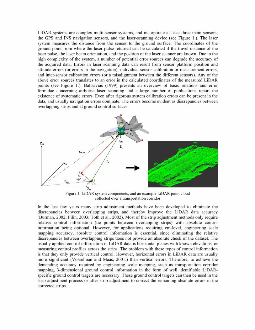
Based on the simulation results, targets were fabricated by the Ohio Department of Transportation to support performance validation experiments. A target is shown in Figure 2. (The GPS antenna in the photo is not part of the LiDAR target; it is used to determine the ground coordinates of the target.)

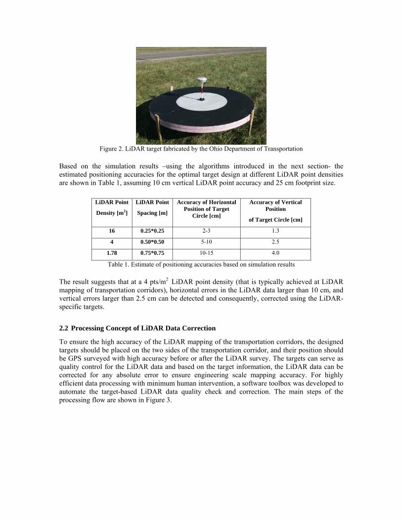
Figure 2. LiDAR target fabricated by the Ohio Department of Transportation

Based on the simulation results –using the algorithms introduced in the next section- the estimated positioning accuracies for the optimal target design at different LiDAR point densities are shown in Table 1, assuming 10 cm vertical LiDAR point accuracy and 25 cm footprint size.

LiDAR Point

Density [m2]

LiDAR Point

Spacing [m]

Accuracy of Horizontal Position of Target

Circle [cm]

Accuracy of Vertical Position

of Target Circle [cm]

16 0.25*0.25 2-3 1.3

4 0.50*0.50 5-10 2.5

1.78 0.75*0.75 10-15 4.0

Table 1. Estimate of positioning accuracies based on simulation results

The result suggests that at a 4 pts/m2 LiDAR point density (that is typically achieved at LiDAR mapping of transportation corridors), horizontal errors in the LiDAR data larger than 10 cm, and vertical errors larger than 2.5 cm can be detected and consequently, corrected using the LiDAR-specific targets.

2.2 Processing Concept of LiDAR Data Correction

To ensure the high accuracy of the LiDAR mapping of the transportation corridors, the designed targets should be placed on the two sides of the transportation corridor, and their position should be GPS surveyed with high accuracy before or after the LiDAR survey. The targets can serve as quality control for the LiDAR data and based on the target information, the LiDAR data can be corrected for any absolute error to ensure engineering scale mapping accuracy. For highly efficient data processing with minimum human intervention, a software toolbox was developed to automate the target-based LiDAR data quality check and correction. The main steps of the processing flow are shown in Figure 3.

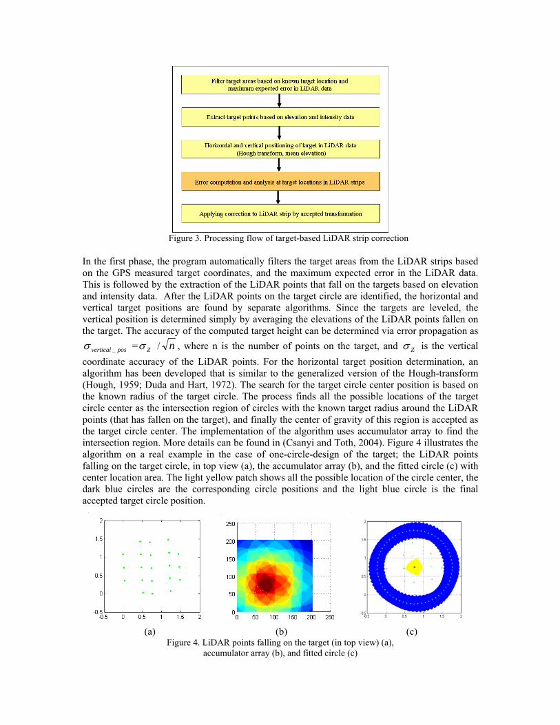
Figure 3. Processing flow of target-based LiDAR strip correction

In the first phase, the program automatically filters the target areas from the LiDAR strips based on the GPS measured target coordinates, and the maximum expected error in the LiDAR data. This is followed by the extraction of the LiDAR points that fall on the targets based on elevation and intensity data. After the LiDAR points on the target circle are identified, the horizontal and vertical target positions are found by separate algorithms. Since the targets are leveled, the vertical position is determined simply by averaging the elevations of the LiDAR points fallen on the target. The accuracy of the computed target height can be determined via error propagation as

posvertical _σ = Zσ / n , where n is the number of points on the target, and Zσ is the vertical coordinate accuracy of the LiDAR points. For the horizontal target position determination, an algorithm has been developed that is similar to the generalized version of the Hough-transform (Hough, 1959; Duda and Hart, 1972). The search for the target circle center position is based on the known radius of the target circle. The process finds all the possible locations of the target circle center as the intersection region of circles with the known target radius around the LiDAR points (that has fallen on the target), and finally the center of gravity of this region is accepted as the target circle center. The implementation of the algorithm uses accumulator array to find the intersection region. More details can be found in (Csanyi and Toth, 2004). Figure 4 illustrates the algorithm on a real example in the case of one-circle-design of the target; the LiDAR points falling on the target circle, in top view (a), the accumulator array (b), and the fitted circle (c) with center location area. The light yellow patch shows all the possible location of the circle center, the dark blue circles are the corresponding circle positions and the light blue circle is the final accepted target circle position.

(a) (b) (c)

Figure 4. LiDAR points falling on the target (in top view) (a), accumulator array (b), and fitted circle (c)

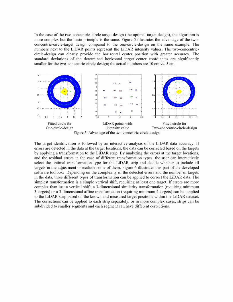
In the case of the two-concentric-circle target design (the optimal target design), the algorithm is more complex but the basic principle is the same. Figure 5 illustrates the advantage of the two-concentric-circle-target design compared to the one-circle-design on the same example. The numbers next to the LiDAR points represent the LiDAR intensity values. The two-concentric-circle-design can clearly provide the horizontal center position with greater accuracy. The standard deviations of the determined horizontal target center coordinates are significantly smaller for the two-concentric-circle-design; the actual numbers are 10 cm vs. 5 cm.

Fitted circle for

One-circle-design LiDAR points with

intensity value Fitted circle for

Two-concentric-circle-design Figure 5. Advantage of the two-concentric-circle-design

The target identification is followed by an interactive analysis of the LiDAR data accuracy. If errors are detected in the data at the target locations, the data can be corrected based on the targets by applying a transformation to the LiDAR strip. By analyzing the errors at the target locations, and the residual errors in the case of different transformation types, the user can interactively select the optimal transformation type for the LiDAR strip and decide whether to include all targets in the adjustment or exclude some of them. Figure 6 illustrates this part of the developed software toolbox. Depending on the complexity of the detected errors and the number of targets in the data, three different types of transformation can be applied to correct the LiDAR data. The simplest transformation is a simple vertical shift, requiring at least one target. If errors are more complex than just a vertical shift, a 3-dimensional similarity transformation (requiring minimum 3 targets) or a 3-dimensional affine transformation (requiring minimum 4 targets) can be applied to the LiDAR strip based on the known and measured target positions within the LiDAR dataset. The corrections can be applied to each strip separately, or in more complex cases, strips can be subdivided to smaller segments and each segment can have different corrections.

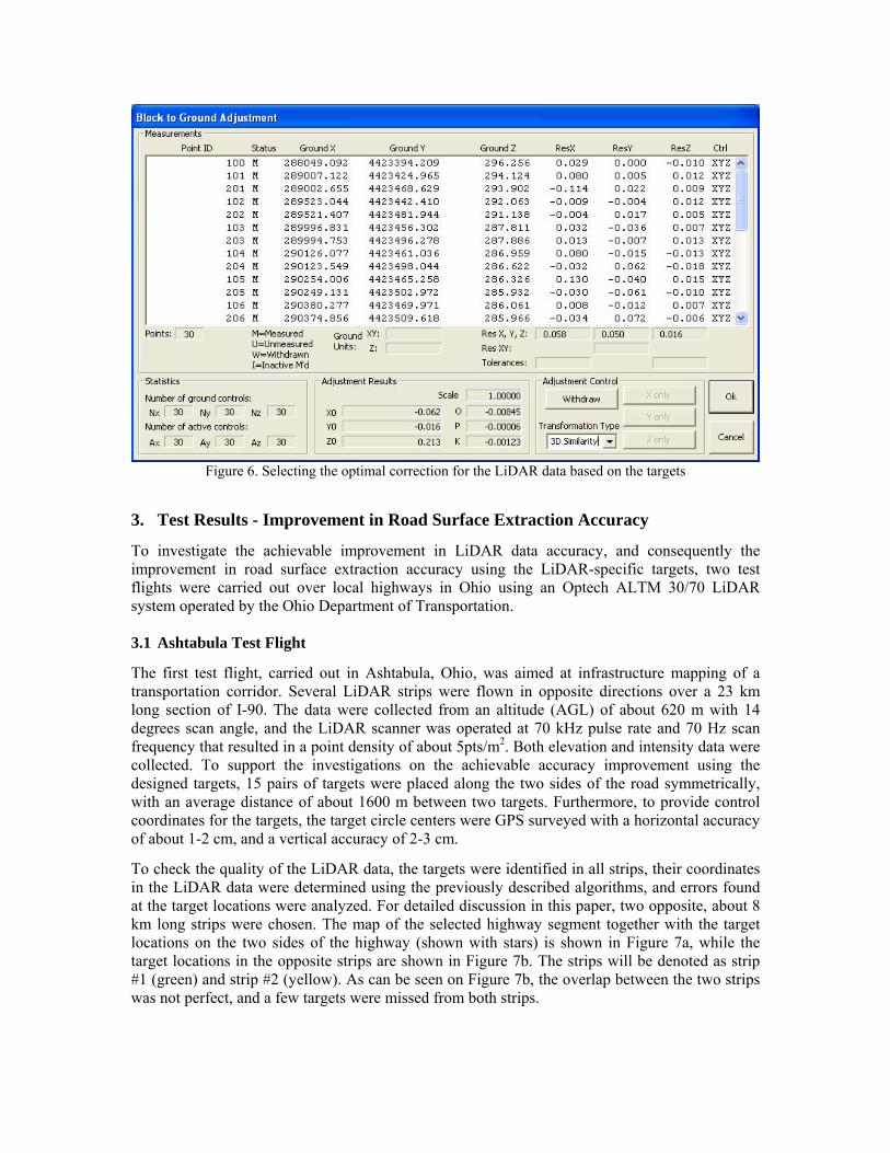
Figure 6. Selecting the optimal correction for the LiDAR data based on the targets

3. Test Results - Improvement in Road Surface Extraction Accuracy

To investigate the achievable improvement in LiDAR data accuracy, and consequently the improvement in road surface extraction accuracy using the LiDAR-specific targets, two test flights were carried out over local highways in Ohio using an Optech ALTM 30/70 LiDAR system operated by the Ohio Department of Transportation. 3.1 Ashtabula Test Flight

The first test flight, carried out in Ashtabula, Ohio, was aimed at infrastructure mapping of a transportation corridor. Several LiDAR strips were flown in opposite directions over a 23 km long section of I-90. The data were collected from an altitude (AGL) of about 620 m with 14 degrees scan angle, and the LiDAR scanner was operated at 70 kHz pulse rate and 70 Hz scan frequency that resulted in a point density of about 5pts/m2. Both elevation and intensity data were collected. To support the investigations on the achievable accuracy improvement using the designed targets, 15 pairs of targets were placed along the two sides of the road symmetrically, with an average distance of about 1600 m between two targets. Furthermore, to provide control coordinates for the targets, the target circle centers were GPS surveyed with a horizontal accuracy of about 1-2 cm, and a vertical accuracy of 2-3 cm.

To check the quality of the LiDAR data, the targets were identified in all strips, their coordinates in the LiDAR data were determined using the previously described algorithms, and errors found at the target locations were analyzed. For detailed discussion in this paper, two opposite, about 8 km long strips were chosen. The map of the selected highway segment together with the target locations on the two sides of the highway (shown with stars) is shown in Figure 7a, while the target locations in the opposite strips are shown in Figure 7b. The strips will be denoted as strip #1 (green) and strip #2 (yellow). As can be seen on Figure 7b, the overlap between the two strips was not perfect, and a few targets were missed from both strips.

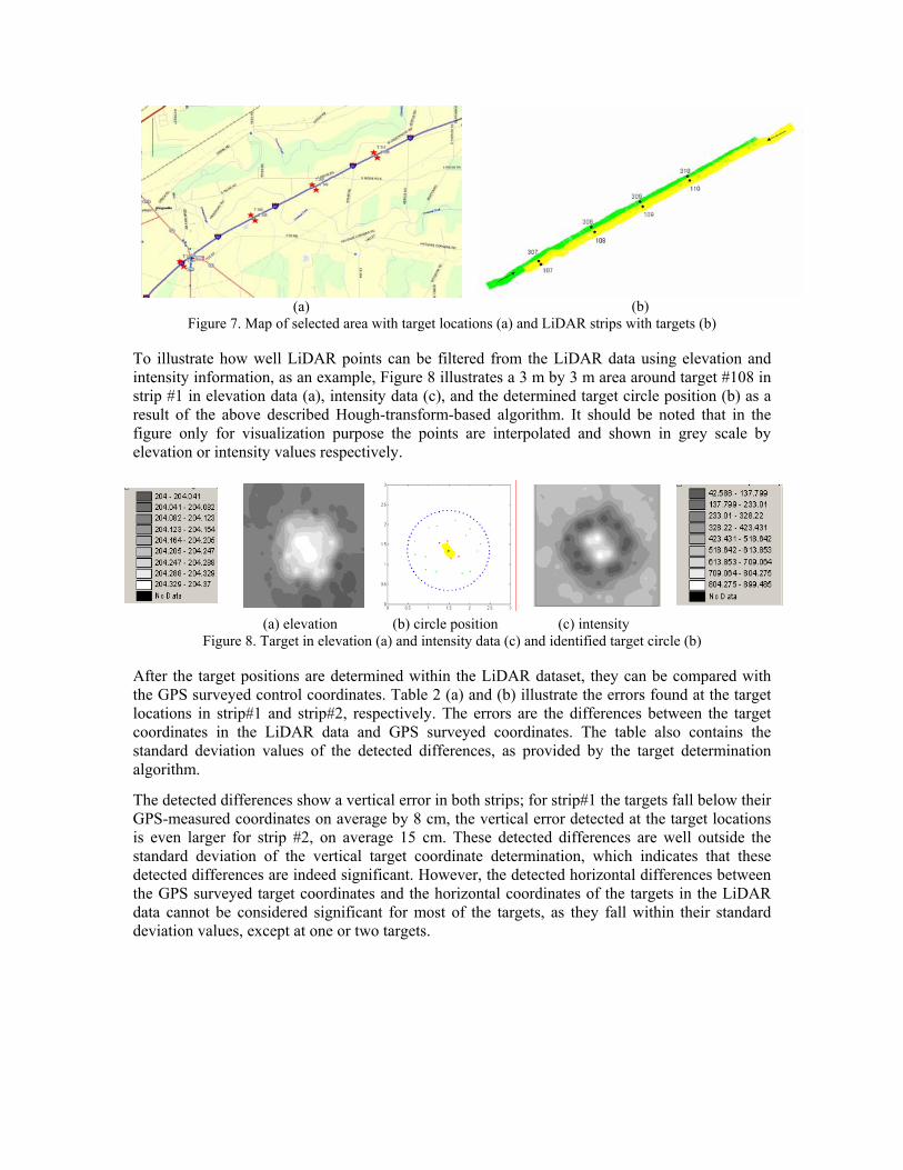
(a)

(b)

Figure 7. Map of selected area with target locations (a) and LiDAR strips with targets (b)

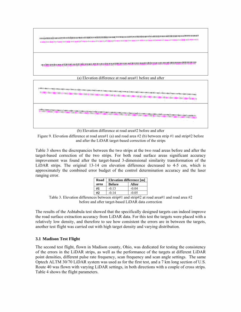
To illustrate how well LiDAR points can be filtered from the LiDAR data using elevation and intensity information, as an example, Figure 8 illustrates a 3 m by 3 m area around target #108 in strip #1 in elevation data (a), intensity data (c), and the determined target circle position (b) as a result of the above described Hough-transform-based algorithm. It should be noted that in the figure only for visualization purpose the points are interpolated and shown in grey scale by elevation or intensity values respectively.

(a) elevation (b) circle position (c) intensity

Figure 8. Target in elevation (a) and intensity data (c) and identified target circle (b)

After the target positions are determined within the LiDAR dataset, they can be compared with the GPS surveyed control coordinates. Table 2 (a) and (b) illustrate the errors found at the target locations in strip#1 and strip#2, respectively. The errors are the differences between the target coordinates in the LiDAR data and GPS surveyed coordinates. The table also contains the standard deviation values of the detected differences, as provided by the target determination algorithm.

The detected differences show a vertical error in both strips; for strip#1 the targets fall below their GPS-measured coordinates on average by 8 cm, the vertical error detected at the target locations is even larger for strip #2, on average 15 cm. These detected differences are well outside the standard deviation of the vertical target coordinate determination, which indicates that these detected differences are indeed significant. However, the detected horizontal differences between the GPS surveyed target coordinates and the horizontal coordinates of the targets in the LiDAR data cannot be considered significant for most of the targets, as they fall within their standard deviation values, except at one or two targets.

Error [m] Standard Deviation [m] Residual [m] Target ID Easting Northing Elevation Easting Northing Elevation Easting Northing Elevation 307 -0.01 0.03 -0.18 0.07 0.07 0.02 -0.05 0.03 -0.03 108 0.05 -0.06 -0.06 0.06 0.08 0.02 0.02 -0.04 0.04 308 0.05 -0.03 -0.07 0.08 0.05 0.02 0.02 -0.01 0.01 109 0.13 0.00 -0.05 0.06 0.08 0.02 0.10 0.03 0.02 309 -0.02 0.00 -0.08 0.08 0.07 0.02 -0.04 0.03 -0.02 110 0.00 0.07 -0.05 0.04 0.05 0.02 -0.02 0.11 0.00 310 0.01 -0.13 -0.06 0.04 0.05 0.02 -0.01 -0.08 -0.02

Mean 0.03 -0.02 -0.08 0.00 0.01 0.00 Std 0.05 0.06 0.05 0.05 0.06 0.03

(a) Error [m] Standard Deviation [m] Residual [m] Target

ID Easting Northing Elevation Easting Northing Elevation Easting Northing Elevation 107 0.04 0.10 -0.11 0.03 0.05 0.02 0.04 0.03 -0.01 108 0.01 -0.03 -0.13 0.04 0.05 0.02 0.01 -0.10 0.02 109 -0.05 0.07 -0.16 0.02 0.01 0.03 -0.05 0.00 -0.02 110 0.10 -0.02 -0.12 0.03 0.04 0.02 0.10 -0.09 0.01 310 -0.02 0.18 -0.17 0.06 0.05 0.02 -0.01 0.11 -0.01

Mean -0.02 0.06 -0.14 0.02 -0.01 0.00 Std 0.06 0.09 0.03 0.06 0.09 0.02

(b)

Table 2. Errors at target locations and residuals after 3D similarity transformation of the strips, in strip #1 (a) and strip #2 (b)

After analyzing the data, a 3-dimensional similarity transformation applied separately for both strips including all the targets was found to be adequate for the correction of the LiDAR data (more details can be found in Csanyi et al., 2005). The last three columns of Table 2 (a) and (b) show the residuals at the target locations after the transformation. The transformation significantly decreased the vertical coordinate errors and they are approximately in the range of the vertical accuracy of the determined target coordinates. The horizontal coordinates did not change much at the targets where the detected differences were originally in the range of the horizontal coordinate determination accuracy; however, at the few targets where the determined errors were significant, an improvement was experienced.

To analyze the impact of the target-based LiDAR data correction on the road surface extraction accuracy, the following method was applied: two 5m by 5m road surface areas were selected from the overlapping areas of the two discussed LiDAR strips, and their discrepancies were checked before and after the target-based correction of the strips. It should be emphasized that the two strips were corrected separately; separate 3D similarity transformations were applied for both strips based on the targets. One area was selected in the vicinity of target #109 (denoted as area#1), and the other one farther from the targets, half way between targets #110 and # 310 (area #2). The road areas were modeled by plane fitting. To illustrate the improvement in road surface extraction accuracy using the targets, Figure 9 (a) and (b) show the elevation difference between the two LiDAR strips at road area#1 and road area#2, respectively, before and after the target-based LiDAR data correction.

(a) Elevation difference at road area#1 before and after

(b) Elevation difference at road area#2 before and after

Figure 9. Elevation difference at road area#1 (a) and road area #2 (b) between strip #1 and strip#2 before and after the LiDAR target-based correction of the strips

Table 3 shows the discrepancies between the two strips at the two road areas before and after the target-based correction of the two strips. For both road surface areas significant accuracy improvement was found after the target-based 3-dimensional similarity transformation of the LiDAR strips. The original 13-14 cm elevation difference decreased to 4-5 cm, which is approximately the combined error budget of the control determination accuracy and the laser ranging error.

Elevation difference [m] Road area Before After #1 -0.13 -0.04 #2 -0.14 -0.05

Table 3. Elevation differences between strip#1 and strip#2 at road area#1 and road area #2 before and after target-based LiDAR data correction

The results of the Ashtabula test showed that the specifically designed targets can indeed improve the road surface extraction accuracy from LiDAR data. For this test the targets were placed with a relatively low density, and therefore to see how consistent the errors are in between the targets, another test flight was carried out with high target density and varying distribution.

3.1 Madison Test Flight

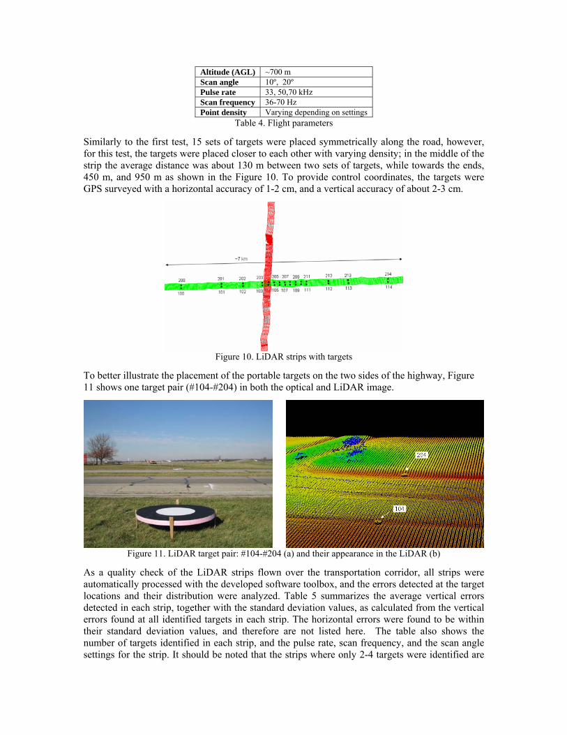
The second test flight, flown in Madison county, Ohio, was dedicated for testing the consistency of the errors in the LiDAR strips, as well as the performance of the targets at different LiDAR point densities, different pulse rate frequency, scan frequency and scan angle settings. The same Optech ALTM 30/70 LiDAR system was used as for the first test, and a 7 km long section of U.S. Route 40 was flown with varying LiDAR settings, in both directions with a couple of cross strips. Table 4 shows the flight parameters.

Altitude (AGL) ~700 m Scan angle 10º, 20º Pulse rate 33, 50,70 kHz Scan frequency 36-70 Hz Point density Varying depending on settings

Table 4. Flight parameters

Similarly to the first test, 15 sets of targets were placed symmetrically along the road, however, for this test, the targets were placed closer to each other with varying density; in the middle of the strip the average distance was about 130 m between two sets of targets, while towards the ends, 450 m, and 950 m as shown in the Figure 10. To provide control coordinates, the targets were GPS surveyed with a horizontal accuracy of 1-2 cm, and a vertical accuracy of about 2-3 cm.

Figure 10. LiDAR strips with targets

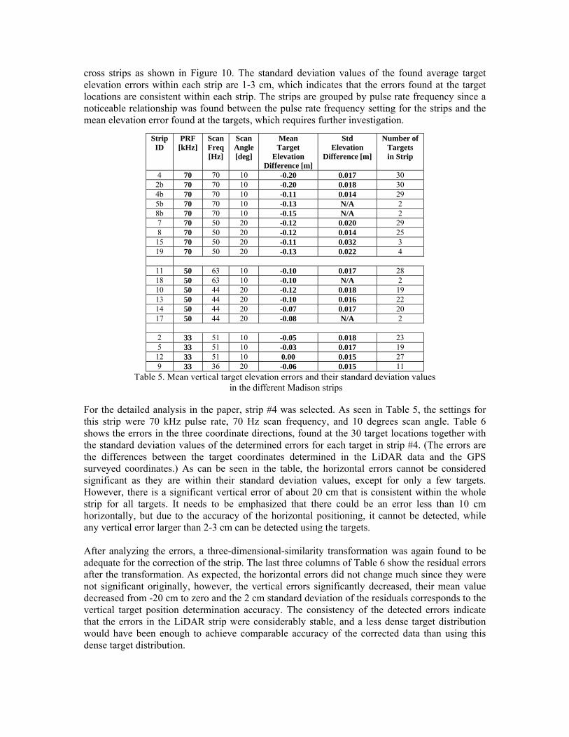
To better illustrate the placement of the portable targets on the two sides of the highway, Figure 11 shows one target pair (#104-#204) in both the optical and LiDAR image.

Figure 11. LiDAR target pair: #104-#204 (a) and their appearance in the LiDAR (b)

As a quality check of the LiDAR strips flown over the transportation corridor, all strips were automatically processed with the developed software toolbox, and the errors detected at the target locations and their distribution were analyzed. Table 5 summarizes the average vertical errors detected in each strip, together with the standard deviation values, as calculated from the vertical errors found at all identified targets in each strip. The horizontal errors were found to be within their standard deviation values, and therefore are not listed here. The table also shows the number of targets identified in each strip, and the pulse rate, scan frequency, and the scan angle settings for the strip. It should be noted that the strips where only 2-4 targets were identified are

Target 104

Target 204

cross strips as shown in Figure 10. The standard deviation values of the found average target elevation errors within each strip are 1-3 cm, which indicates that the errors found at the target locations are consistent within each strip. The strips are grouped by pulse rate frequency since a noticeable relationship was found between the pulse rate frequency setting for the strips and the mean elevation error found at the targets, which requires further investigation.

Strip

ID PRF [kHz]

Scan Freq [Hz]

Scan Angle [deg]

Mean Target

Elevation Difference [m]

Std Elevation

Difference [m]

Number of Targets in Strip

4 70 70 10 -0.20 0.017 30 2b 70 70 10 -0.20 0.018 30 4b 70 70 10 -0.11 0.014 29 5b 70 70 10 -0.13 N/A 2 8b 70 70 10 -0.15 N/A 2 7 70 50 20 -0.12 0.020 29 8 70 50 20 -0.12 0.014 25

15 70 50 20 -0.11 0.032 3 19 70 50 20 -0.13 0.022 4

11 50 63 10 -0.10 0.017 28 18 50 63 10 -0.10 N/A 2 10 50 44 20 -0.12 0.018 19 13 50 44 20 -0.10 0.016 22 14 50 44 20 -0.07 0.017 20 17 50 44 20 -0.08 N/A 2 2 33 51 10 -0.05 0.018 23 5 33 51 10 -0.03 0.017 19

12 33 51 10 0.00 0.015 27 9 33 36 20 -0.06 0.015 11

Table 5. Mean vertical target elevation errors and their standard deviation values in the different Madison strips

For the detailed analysis in the paper, strip #4 was selected. As seen in Table 5, the settings for this strip were 70 kHz pulse rate, 70 Hz scan frequency, and 10 degrees scan angle. Table 6 shows the errors in the three coordinate directions, found at the 30 target locations together with the standard deviation values of the determined errors for each target in strip #4. (The errors are the differences between the target coordinates determined in the LiDAR data and the GPS surveyed coordinates.) As can be seen in the table, the horizontal errors cannot be considered significant as they are within their standard deviation values, except for only a few targets. However, there is a significant vertical error of about 20 cm that is consistent within the whole strip for all targets. It needs to be emphasized that there could be an error less than 10 cm horizontally, but due to the accuracy of the horizontal positioning, it cannot be detected, while any vertical error larger than 2-3 cm can be detected using the targets. After analyzing the errors, a three-dimensional-similarity transformation was again found to be adequate for the correction of the strip. The last three columns of Table 6 show the residual errors after the transformation. As expected, the horizontal errors did not change much since they were not significant originally, however, the vertical errors significantly decreased, their mean value decreased from -20 cm to zero and the 2 cm standard deviation of the residuals corresponds to the vertical target position determination accuracy. The consistency of the detected errors indicate that the errors in the LiDAR strip were considerably stable, and a less dense target distribution would have been enough to achieve comparable accuracy of the corrected data than using this dense target distribution.

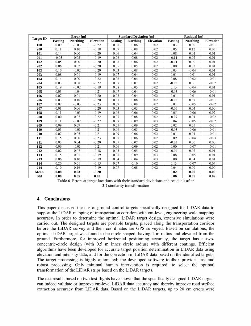
Error [m] Standard Deviation [m] Residual [m] Target ID Easting Northing Elevation Easting Northing Elevation Easting Northing Elevation

100 0.09 -0.03 -0.22 0.08 0.06 0.02 0.03 0.00 -0.01 200 0.11 0.10 -0.18 0.07 0.08 0.02 0.05 0.12 0.03 101 0.14 0.00 -0.20 0.06 0.04 0.02 0.08 0.01 0.01 201 -0.05 0.02 -0.19 0.06 0.08 0.02 -0.11 0.02 0.01 102 0.05 0.00 -0.20 0.08 0.06 0.02 -0.01 0.00 0.01 202 0.06 0.02 -0.20 0.05 0.05 0.02 0.00 0.02 0.01 103 0.10 -0.02 -0.20 0.03 0.08 0.02 0.03 -0.04 0.01 203 0.08 0.01 -0.19 0.07 0.04 0.03 0.01 -0.01 0.01 104 0.14 0.00 -0.22 0.06 0.04 0.02 0.08 -0.02 -0.01 204 0.03 0.08 -0.22 0.07 0.07 0.02 -0.03 0.06 -0.02 105 0.19 -0.02 -0.19 0.08 0.05 0.02 0.13 -0.04 0.01 205 0.03 -0.04 -0.21 0.07 0.04 0.02 -0.03 -0.06 -0.01 106 0.07 0.01 -0.20 0.03 0.04 0.02 0.01 -0.01 0.01 206 0.03 0.10 -0.20 0.03 0.08 0.02 -0.03 0.07 -0.01 107 0.07 -0.03 -0.23 0.09 0.08 0.02 0.01 -0.05 -0.02 207 0.01 0.06 -0.20 0.03 0.03 0.02 -0.05 0.04 0.00 108 0.11 -0.03 -0.19 0.06 0.06 0.02 0.05 -0.06 0.02 208 0.00 0.07 -0.22 0.07 0.08 0.02 -0.07 0.04 -0.02 109 0.11 -0.02 -0.22 0.07 0.09 0.03 0.04 -0.05 -0.02 209 0.09 0.09 -0.21 0.05 0.09 0.02 0.02 0.05 -0.01 110 0.03 -0.03 -0.21 0.06 0.05 0.02 -0.03 -0.06 -0.01 210 0.07 0.05 -0.21 0.09 0.06 0.02 0.01 0.01 -0.01 111 0.15 0.00 -0.23 0.08 0.06 0.02 0.09 -0.04 -0.03 211 0.03 0.04 -0.20 0.05 0.07 0.02 -0.03 0.00 0.00 112 0.06 -0.03 -0.21 0.06 0.09 0.02 0.00 -0.07 -0.01 212 0.02 0.07 -0.18 0.03 0.05 0.02 -0.04 0.02 0.01 113 0.15 0.01 -0.19 0.08 0.09 0.03 0.08 -0.05 0.01 213 0.06 0.10 -0.19 0.04 0.04 0.03 0.00 0.04 0.01 114 0.20 0.01 -0.15 0.07 0.10 0.02 0.13 -0.07 0.04 214 0.10 0.16 -0.19 0.07 0.08 0.02 0.04 0.09 0.00

Mean 0.08 0.03 -0.20 0.02 0.00 0.00 Std 0.06 0.05 0.02 0.06 0.05 0.02

Table 6. Errors at target locations with their standard deviations and residuals after 3D similarity transformation

4. Conclusions

This paper discussed the use of ground control targets specifically designed for LiDAR data to support the LiDAR mapping of transportation corridors with cm-level, engineering scale mapping accuracy. In order to determine the optimal LiDAR target design, extensive simulations were carried out. The designed targets are portable targets, placed along the transportation corridor before the LiDAR survey and their coordinates are GPS surveyed. Based on simulations, the optimal LiDAR target was found to be circle-shaped, having 1 m radius and elevated from the ground. Furthermore, for improved horizontal positioning accuracy, the target has a two-concentric-circle design (with 0.5 m inner circle radius) with different coatings. Efficient algorithms have been developed for accurate target position determination in LiDAR data using elevation and intensity data, and for the correction of LiDAR data based on the identified targets. The target processing is highly automated; the developed software toolbox provides fast and robust processing. Only minimal human intervention is required; to select the optimal transformation of the LiDAR strips based on the LiDAR targets.

The test results based on two test flights have shown that the specifically designed LiDAR targets can indeed validate or improve cm-level LiDAR data accuracy and thereby improve road surface extraction accuracy from LiDAR data. Based on the LiDAR targets, up to 20 cm errors were

detected in the LiDAR data collected over transportation corridors that was corrected using the LiDAR-specific targets. The results have shown that at a LiDAR point density of 5 pts/m2, 10 cm horizontal accuracy and 2-3 cm vertical accuracy of the extracted road surface can be achieved using the designed targets. To provide this high level of accuracy, a dense and well-distributed network of targets is needed. Acknowledgements

The author would like to thank the Ohio Department of Transportation for manufacturing the LiDAR targets based on the simulation results, and providing essential data for this research.

References Baltsavias, E.P. (1999). Airborne laser scanning: basic relations and formulas. ISPRS Journal of

Photogrammetry & Remote Sensing Vol. 54, pp. 199-214.

Burman, H. ,2002. Laser strip adjustment for data calibration and verification. International Archives of Photogrammetry and Remote Sensing, 34 (Part 3A): 67-72.

Csanyi N, C. Toth, D. Grejner-Brzezinska, 2005. Using LiDAR-specific ground targets: a performance analysis, ISPRS WGI/2 Workshop on 3D Mapping from InSAR and LiDAR, Banff, Alberta, Canada, 7-10 June, CD-ROM.

Csanyi N, C. Toth, D. Grejner-Brzezinska, and J. Ray, 2005. Improving LiDAR data accuracy using LiDAR-specific ground targets, ASPRS Annual Conference, Baltimore, MD, March 7-11, CD-ROM.

Csanyi N, C. Toth, 2004. On using LiDAR-specific ground targets, ASPRS Annual Conference, Denver, CO, May 23-28, CD-ROM.

Duda R. O., Hart P. E., 1972. Use of the Hough Transformation to detect lines and curves in pictures, Graphics and Image processing, 15: 11-15.

Filin, S., 2003. Analysis and implementation of a laser strip adjustment model. International Archives of Photogrammetry and Remote Sensing, 34 (Part 3/W13): 65-70.

Hough P.V.C., 1959. Machine analysis of bubble chamber pictures, International Conference on High Energy Accelerators and Instrumentation, CERN.

Toth C., N. Csanyi, and D.Grejner-Brzezinska, 2002. Automating the calibration of airborne multisensor imaging systems, Proc. ACSM-ASPRS Annual Conference, Washington, DC, April 19-26, CD ROM.

Toth, C. 2004: Future Trends in LiDAR, Proc. ASPRS 2004 Annual Conference, Denver, CO, May 23-28, CD-ROM.

Renslow, M., 2005. The Status of LiDAR Today and Future Directions, 3D Mapping from InSAR and LiDAR, ISPRS WG I/2 Workshop, Banff, Canada, June 7-10, CD-ROM.

Vosselman, G. and H.-G. Maas, 2001. Adjustment and filtering of raw laser altimetry data. Proceedings OEEPE Workshop on Airborne Laserscanning and Interferometric SAR for Detailed Elevation Models. OEEPE Publications no. 40: 62-72.