Technology Assimilation and Growth

Tsz-Nga WongDepartment of Economics

Washington University at St. Louis, USA

Chong K. YipDepartment of Economics

The Chinese University of Hong Kong, Hong Kong

January 29, 2009

Abstract

This paper examines the effect of technology adoption on economic devel-opment in a standard overlapping generations model. The key to successfultechnology adoption is a country’s ability to technology assimilation. If tech-nology assimilation is weak, then wages are not sufficient to support capitalused by the advanced capital-intensive technology. As a result, future pro-duction declines and a poverty trap is formed. If technology assimilationis strong, then converging to the steady state of the rich is almost a sureoutcome through technology adoption.Key Words: technology assimilation, elasticity of substitution, poverty trap.JEL Classification Codes: O110, O330, O410.

Address for Correspondence: Chong K. Yip, Department of Economics, The Chi-nese University of Hong Kong, Shatin, Hong Kong. Tel: (852) 26098187, Fax: (852)26035805, Email: chongkeeyip@cuhk.edu.hk.

1 Introduction

An important question in macroeconomics is why there are large disparities in per

capita income across countries. A common answer offered by economists is the

differences in production technologies and knowledge.1 In standard models of eco-

nomic growth, productivity is usually indexed by a single coefficient independent of

factor inputs. Unless the improvements are country-specific, technological improve-

ment in one country should then also improve productivity of the others. Given

the vast examples of technological transfer across countries, how can we avoid the

counterfactual prediction of standard growth models?

Existing literature offers alternative explanations and here we highlight two

strands. One well-developed strand of literature emphasizes that technological

transfer across countries is subject to different barriers of adoption. For instance,

Parente and Prescott (1994) models the barrier to technology transfer as a cost of its

adoption. Chen et al (2002) specifies the barriers of technology adoption in terms of

search and entry frictions in the labor market. Other interesting work in this area

includes the quality-ladder model of Segerstrom et al (1990), the costly-imitation

models of technology diffusion by Grossman and Helpman (1991) and Barro and

Sala-i-Martin (1997), the monopoly model of rent-seeking by Parente and Prescott

(1999) and the industrial transformation model by Wang and Xie (2004). Allowing

for free and instant technology transfer across countries, another popular strand of

literature abandons the assumption that technological improvement affects all parts

of the production structure to the same extent. Instead it focuses on the "appro-

priateness" of technology and the main idea is that "countries with different factor

endowments should choose different technologies." [Caselli and Coleman (2006),

p.501] The origin of the appropriate-technology literature goes back to the work

of Atkinson and Stiglitz on the "localised technology." Productivity improvement

is based on learning by doing on the firm’s current production technique which is

specified by a given capital-labor ratio. Recently, Basu and Weil (1998) extends

the Atkinson-Stiglitz model by considering that technological improvement are not

only for a specific combination of capital and labor but also of similar techniques.2

1See Prescott (1998) for a discussion. Empirically, it is found that cross-country differences intotal factor productivity are significant (e.g., Hall and Jones 1999).

2According to Basu and Weil (1998), it is in the neighborhood of γ of the specific capital-laborratio.

1

The North-South model of Acemoglu and Zilibotti (2001) differs from Atkinson and

Stiglitz (1969) and Basu and Weil (1998) by focusing on skilled and unskilled labor

instead of capital intensities. More importantly, technological improvement is an

outcome of optimizing behavior of firms and the results of productivity differences

followed from the fact that there is a technology-skill mismatch between the North

and the South.3

Our paper belongs to the latter strand of literature on appropriate technology.

The main motivation of our work is the well-documented phenomenon of technology

adoption. Consider the following quotation from the classic development textbook

of Kindleberger (1956):

"...whether countries at early stages of development, ..., should take advantage of

the modern technology developed by advanced countries, ..., or whether they should

devise a technology of their own or use production methods which are obsolete in

countries abroad." (p. 249)

We believe that the answer depends on the ability of technology assimilation of the

developing countries. Also, as Lin (2007) observes:

"... enterprises in developing countries can fully utilise the industrial and techno-

logical gap with developed countries and acquire industrial and technological inno-

vations that are consistent with their new comparative advantage through learning

and borrowing from developed countries, especially from those countries whose stage

of development is higher than but not far away from theirs." (p.32)

Two examples are cited by Lin in his Marshall lecture. The first one was the expe-

rience of the continental countries in Western Europe who adopted the technology

from the United Kingdom in the nineteenth century. But the same industrial strat-

egy did not work for the poorer countries in Eastern Europe. The second example

was the post-World War II development of the four East Asian NIEs (Hong Kong,

Singapore, South Korea and Taiwan). They borrowed technology from Japan in-

stead of USA and Western Europe and were successful. In this paper, we propose

the concept of technology assimilation to help to understand the above examples.4

3In the words of Acemoglu and Zilibotti (2001), it is "because unskilled workers in the Southperform some of the tasks performed by skilled worker in the North." (p.566)

4Lin (2007) discusses these examples in terms of different development policies pursued bythe governments: the comparative advantage-defying strategy versus the comparative advantage-following strategy. Matching our results with his discussion, it seems that technology assimilationis an important condition for a successful comparative advantage-following policy.

2

Also, recall the farmer example considered in Basu and Weil (1998):

"In India, fields are harvested by bands of sweating workers, bending to use their

scythes. In the United States one farmer does the same work, riding in an air-

conditioned combine. Yet an economist might argue that the two countries do have

access to the same technology and simply choose different combinations of inputs

(points along an isoquant) due to differences in factor prices." (p.1025)

Then Basu and Weil (1998) proposes an explanation by agreeing that "all technol-

ogy is freely available and instantly transferred. But a country may nonetheless

refrain from using a new technology until it reaches a level of development at which

this technology would be appropriate to its needs." (p. 1027) We instead explain

the farmer example in terms of technology assimilation, i.e., Indian farmers are un-

able to assimilate the combine technology used by the US farmer.5 Moreover, our

story of technology assimilation corroborates the empirical work by Los and Tim-

mer (2005) on the Basu-Weil (BW) model of appropriate technology. According to

Los and Timmer (2005), "[a]n important assumption in the BW model is that new

knowledge generated in one country is immediately available to all other countries."

(p.519) Following the decomposition technique based on data envelopment analy-

sis developed by Kumar and Russell (2002), they conclude that "for the original

BW model to have empirical relevance, the assumption of immediate spillovers of

appropriate technology needs to be relaxed. Assimilation of technologies new to

a country is a costly and slow process." (Los and Timmer, 2005, p.529) Thus, we

believe that understanding the role of technology assimilation is a challenging and

important task of the appropriate technology literature.

Our paper contributes to the literature of appropriate technology by explicitly

modelling the mechanism of technology assimilation. Specifically, the appropriate-

ness of technology depends on the ability of assimilation of the backward country.

In order to understand how technology assimilation affects the development process,

we build an adaptability function in normalized constant-elasticity-of-substitution

(CES) form for its measurement.6 Following Basu and Weil (1998), we index tech-

5Our concept of technology assimilation can be regarded as a formalization of the idea of theintermediate technology proposed by Schumacher (1973). According to Schumacher, capital-intensive processes are unproductive in developing countries because they are "lack of marketingand financial infrastructure, inappropriate inputs, and untrained workers." (Basu and Weil, 1998,p.1026) In our understanding, the lack of these factors is the cause for the failure of technologyassimilation.

6For an introduction of the normalized CES function, see Klump and de la Grandville (2000).

3

nology in terms of the capital-labor ratio. As a result, the degree of technology

assimilation is measured by the elasticity of substitution between the domestic and

foreign capital intensities in the adaptability function. Different from the existing

work such as Basu and Weil (1998) and Acemoglu and Zilibotti (2001), we do not

just look at the two extreme cases: appropriate technology versus inappropriate

technology.7 Our adaptability function highlights the interaction of technologies

between the advanced country (the North) and the backward country (the South).

It provides a much wider spectrum of appropriate technology and fills in the in-

termediate cases that are overlooked in the literature. An interesting but realistic

prediction from our model is that the lower the degree of technological assimilation,

the more likely that borrowing technology would lead to a poverty trap so that

the South is worse off. This may help to understand why developing countries

sometimes refuse to import advanced foreign production technologies.

The organization of the paper is as follows. The autarkic model is developed in

the next section so as to highlight the structure of the economy and the character-

istics of the adaptability function for technology assimilation. Section 3 consider

the extreme case where technology assimilation is absent so that poverty trap is

an outcome from technology borrowing. Section 4 studies the full version of the

North-South model of technology assimilation. Finally, there is a fifth concluding

section.

2 The Autarkic Model

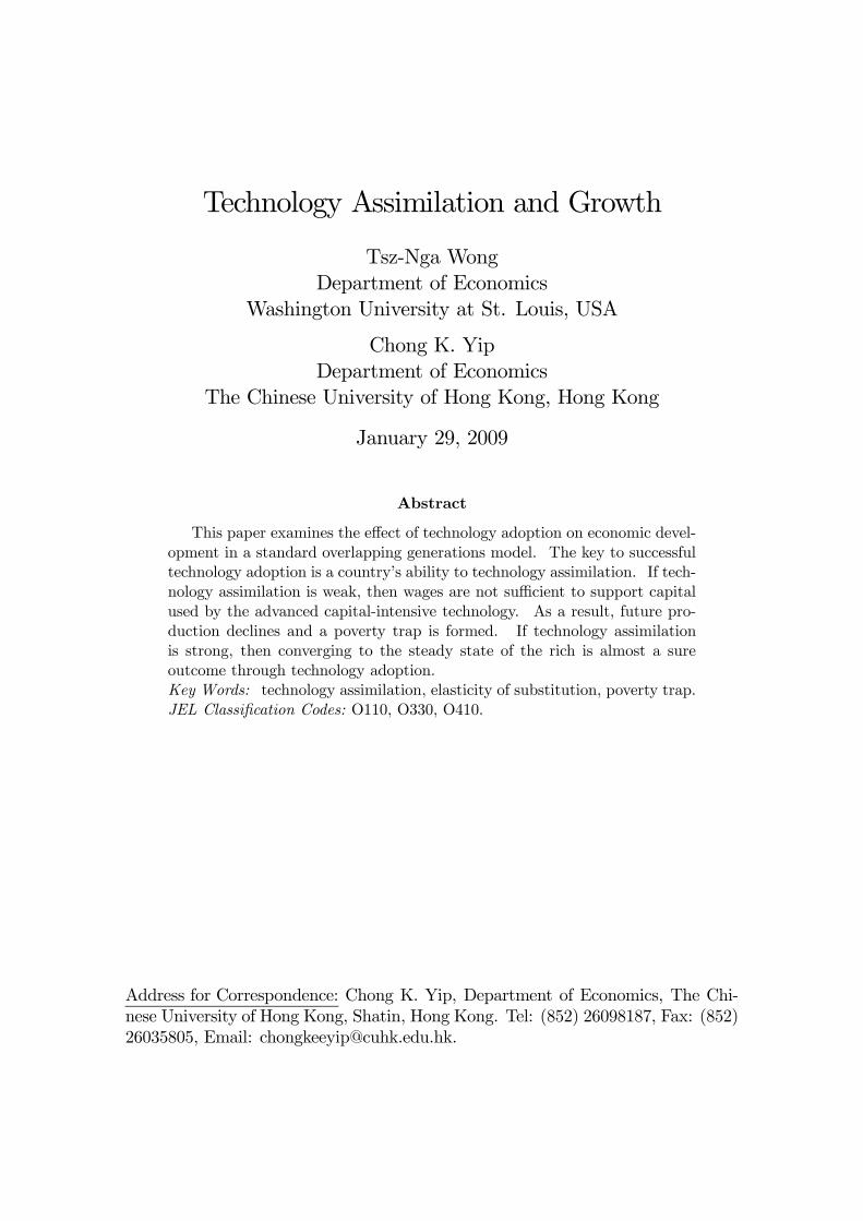
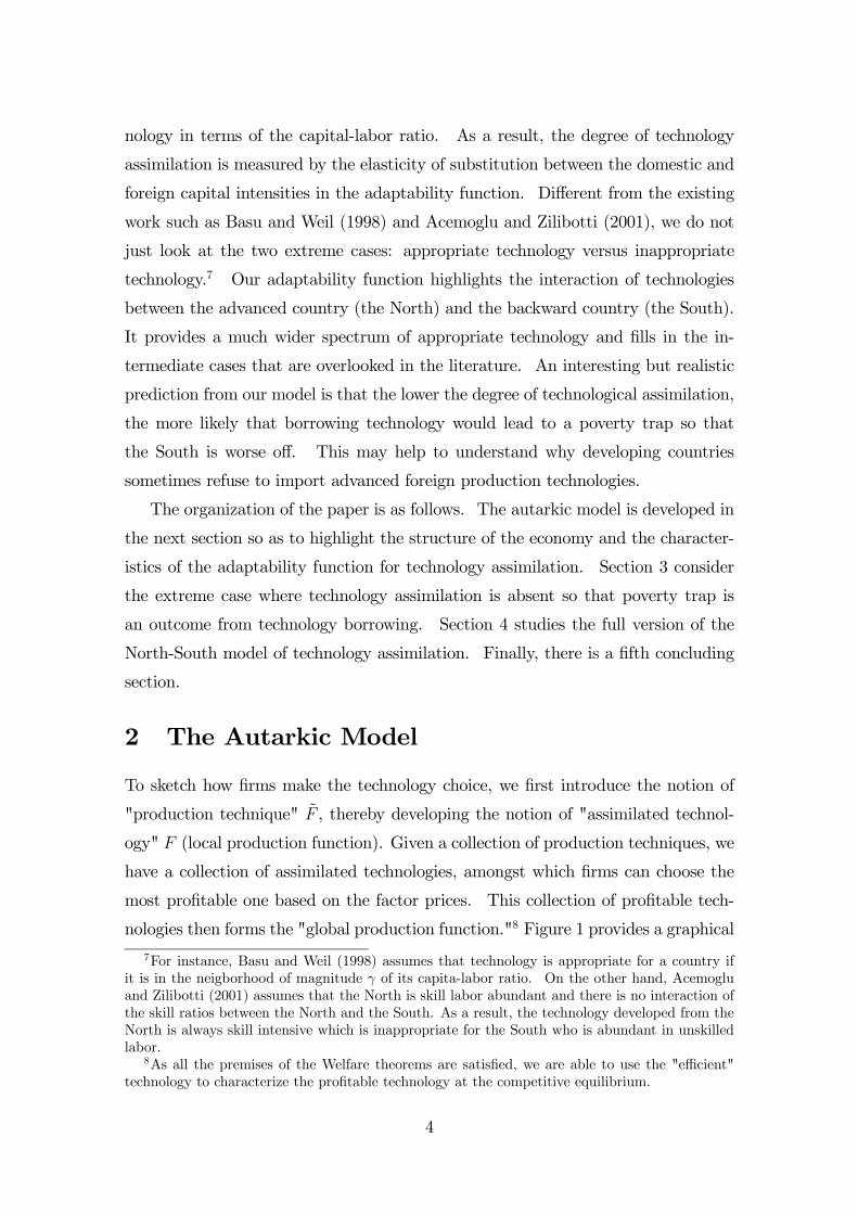
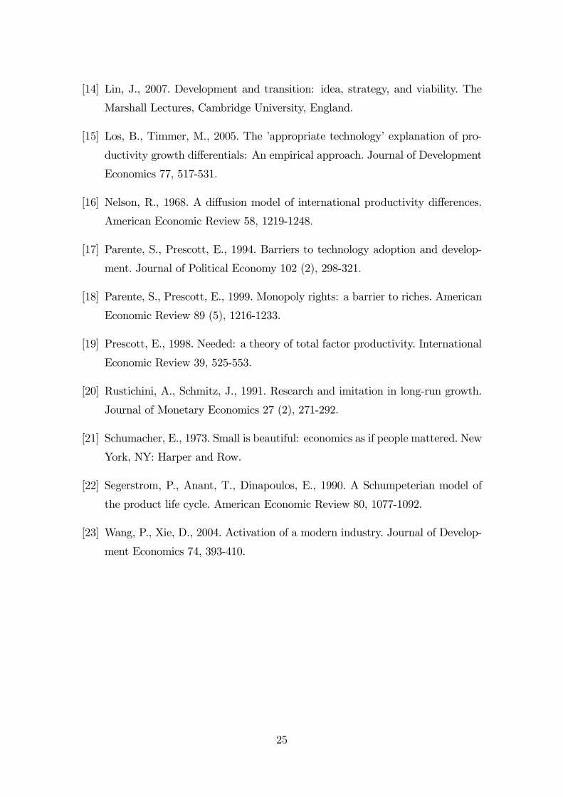
To sketch how firms make the technology choice, we first introduce the notion of

"production technique" F̃ , thereby developing the notion of "assimilated technol-

ogy" F (local production function). Given a collection of production techniques, we

have a collection of assimilated technologies, amongst which firms can choose the

most profitable one based on the factor prices. This collection of profitable tech-

nologies then forms the "global production function."8 Figure 1 provides a graphical

7For instance, Basu and Weil (1998) assumes that technology is appropriate for a country ifit is in the neigborhood of magnitude γ of its capita-labor ratio. On the other hand, Acemogluand Zilibotti (2001) assumes that the North is skill labor abundant and there is no interaction ofthe skill ratios between the North and the South. As a result, the technology developed from theNorth is always skill intensive which is inappropriate for the South who is abundant in unskilledlabor.

8As all the premises of the Welfare theorems are satisfied, we are able to use the "efficient"technology to characterize the profitable technology at the competitive equilibrium.

4

representation of these concepts.9

2.1 Technique, Technology, and Production Function

To be more specific, for a given production technique, output in our economy is

produced using two factors inputs: capital K and labor N . Following Jones (2005),

a particular production technique i is defined by two parameters, ai and bi, so that

the output Y can be written as10

Y = F̃ (aiK, biN). (1)

It is assumed that F̃ is a constant-returns-to-scale (CRTS) function. Rewriting F̃

in per capita terms, we have

y ≡ Y/N = biF̃ (aiK

biN, 1) ≡ biF̃ (

aibik, 1). (2)

Define ki ≡ bi/ai, then the expression becomes11

y = biF̃ (k

ki, 1). (3)

With the normalization that F̃ (1, 1) = 1, we have k = ki and hence y = bi = b so

that the production technique is indexed by ki and bi instead. Given our focus is

on technology assimilation, we assume F̃ to take the Leontief form:

y = bimin(k

ki, 1).

Thus, output is at its highest level when k = ki. If k < ki, firms have idle labor

so that the production technique is not "appropriate." As a result, firms would try

their best to make use of it by looking for or adapting a "better" technique. Let

σ be a measure of technology assimilation that captures how well firms can utilize

their idle labor given a production technique. In other words, countries can be char-

acterized and compared according to their ability of technology assimilation, i.e.,

the parameter σ. To this end, the normalized constant-elasticity-of-substitution

9In Figure 1, the production "technique" is the Leontief kink; while the "assimilated technol-ogy" is the CES curve developed from the kink point. The "(global) production function" is theenvelope of all the CES curves.10Jones (2005) calls F̃ below "the local production function associated with technique i."11Although strictly speaking ki is not capital intensity, our concept of technological appropri-

ateness is closely related to the capital intensity k. To facilitate model solving, we simply followBasu and Weil (1998) to index technology by the capital-labor ratio.

5

(CES) function introduced by Klump and de la Grandville (2000) provides us with

the perfect specification. Thus, we assume the "assimilated" output level is given

by the following adaptability function Q:12

Y = F (aiK, biN, σ) ≡ biQ(K/ki, N, σ) ≡ biAhα (K/ki)

σ−1σ + (1− α)N

σ−1σ

i σσ−1

.

(4)

In per capita terms, we have

y(k/ki, σ) = biq(k/ki, σ) = biAhα (k/ki)

σ−1σ + (1− α)

i σσ−1

. (5)

Before proceeding further, let us take a closer look at the adaptability function

q and understand some of its properties. First of all, when there is no assimilation,

we expect Q to take the Leontief form, i.e., Q = K/ki, so that there exists a

lower bound for q such that k/ki ≤ q(k/ki, σ).13 Secondly, it is expected that

more capital and higher σ improve technology assimilation so that ∂q/∂k > 0 and

∂q/∂σ > 0. Thirdly, when k = ki, we should have y = bi = b so that q(1, σ) = 1.

This in turn implies that A = 1. Fourthly, when k = 0, we should get y = 0 so

that q(0, σ) = 0. This in turn implies that σ cannot exceed unity. Finally, with

maximum adaptability σ = 1, q takes the Cobb-Douglas form and we have

q(k/ki, 1) = (k/ki)α.

We interpret it is the case that firms can perform perfect technology assimilation,

so they can produce at the highest output level where y = bi = b. Equivalently we

have

biq(k/ki, 1) = b or b/bi = (k/ki)α.

Thus the intensive local production function with a given "technology" ki or simply

the production technology ki is

y(k/ki, σ) = biq(k/ki, σ) = bihα (k/ki)

σ−1σ + (1− α)

i σσ−1

. (6)

The corresponding isoquants are depicted in Figure 1.

Next, we want to characterize the collection of efficient technology, which is the

technology ki maximizing y given k. Let ρ be the output ratio of technology ki

12The derivation details of the normalized CES adaptability function are given in the Appendix6.1.13In this case, the production technique and the assimilated output function coincide and is

studied in Jones (2005).

6

over technology k:

ρ(k, ki, σ) ≡y(k/ki, σ)

y(1, σ)=

hα (k/ki)

σ−1σ + (1− α)

i σσ−1

(k/ki)α.

Direct differentiation with respect to ki yields

dρ

dki=

α (1− α)hα (k/ki)

σ−1σ + (1− α)

i 1σ−1

(k/ki)1+α

h(k/ki)

σ−1σ − 1

i> 0 iff ki < k.

So output is at its highest level whenever ki = k. Hence an efficient technology

given capital per labor k is simply the technology k. With the exception for the

case where σ = 1, adopting the "right" technique (technology k) is always more

efficient than assimilating a "wrong" technique (technology other k) for a firm. It

thus hints that when firms are induced to use a "wrong" technique, a poverty trap

can result. Next, the convex hull of efficient technologies is the "global production

function". As the number of techniques available increases, the global production

function f can be approximated by a Cobb-Douglas production function, i.e.,14

y = f(k) = zkα, (7)

where z ≡ biki−α is a constant that measures the "productivity". The global

production function is an envelope of all the local production functions of technology

ki.15

Turning to the preference side, we consider a discrete-time economy populated

by an infinite sequence of two-period lived, overlapping generations. At each date

a set of young agents is born and all agents are risk neutral, and care only about old

age consumption. Hence all young period income is saved and invested in capital

formation. Each agent is endowed with one unit of labor when young, which is

supplied inelastically and earns a wage income w. Agents are retired when old and

agents other than the initial old have no endowment of capital or the final good at

any date. We assume that the initial old of a country is each endowed with K0

units of capital.

14See Jones (2005) for the technical details. Such a production function is called the globalproduction function.15The isoquant associated with the global production function is given in Figure 1.

7

2.2 The Autarkic Steady State

We assume that there are competitive rental markets for capital and labor and

that factors of production are immobile across the border. There is no population

growth and capital depreciates completely in production each period. Standard

marginal productivity conditions yield

r = fk(k) = αzkα−1, (8)

w = f(k)− kfk(k) = (1− α)zkα. (9)

Equilibrium requires that savings equal investment in each period:

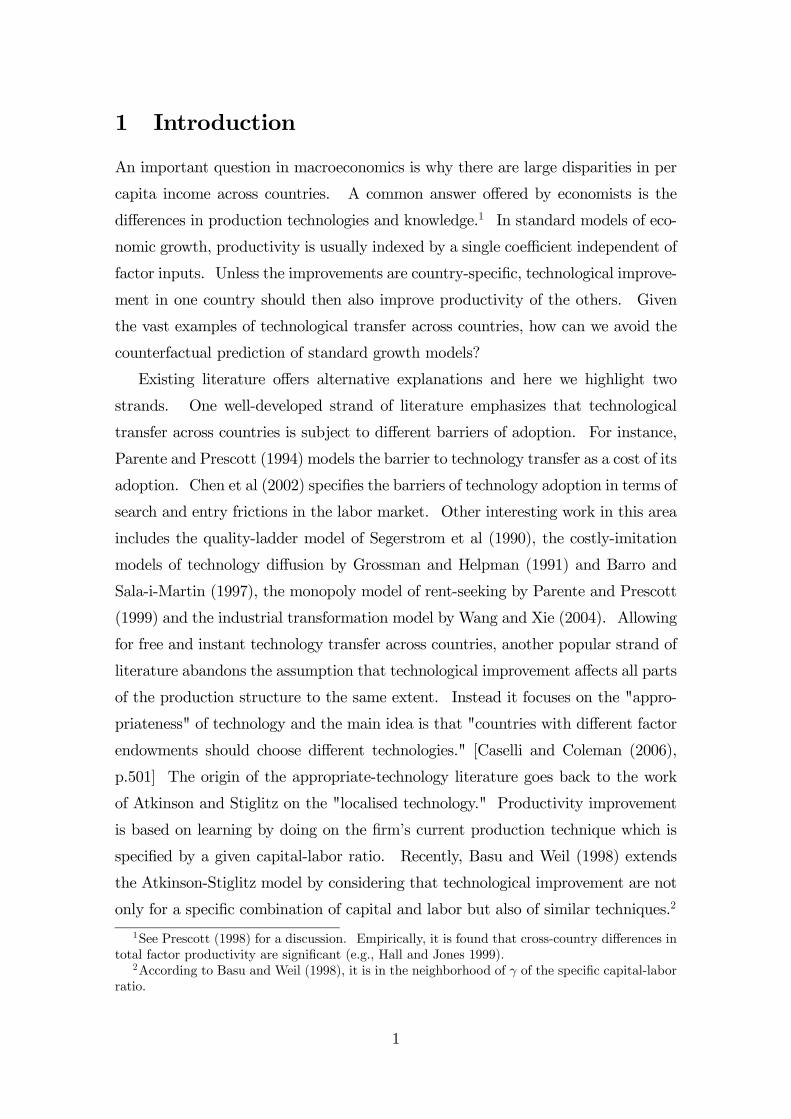
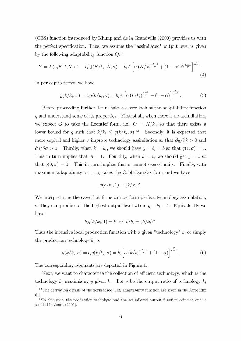
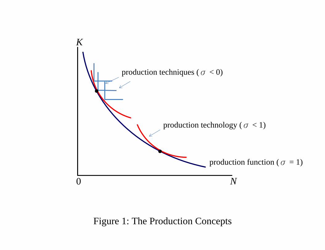
kt+1 = w(kt). (10)

The unique fixed point given by (10) is

k∗A = w(k∗A) or k∗A = [(1− α)z]1

1−α . (11)

According to (9), w(kt) is increasing and concave. In addition, we have limk→0w0(k) <

1 and limk→∞(kt+1/kt) > 1 so that the fixed point is globally stable. Thus the law-

of-motion equation (10) implies that the convergence toward the fixed point k∗Amust be monotone. We depict the fixed point in Figure 2.

We are now ready to characterize the steady state in autarky. In order to have

the capital market equilibrium k∗A to be the steady state, we must make sure that

k∗A is also an equilibrium for the production technique ki = k∗A, i.e., firms have no

incentive to switch to other production techniques. With the production technology

ki, the corresponding wage level is given by

w(k, ki, σ) = (1− α)bihα (k/ki)

σ−1σ + (1− α)

i 1σ−1

.

Since ki = k = k∗A at the fixed point, we have

w(k∗A, k∗A, σ) = (1− α)bi = (1− α)z (k∗A)

α

so that the same equilibrium is obtained. Thus we conclude that k∗A is a steady

state at which both the level of capital stock as well as the production technique do

not change. We also note that k∗A is independent of the adaptability parameter σ.

This is an implication of the fact that the global production function is an envelope

of all local production functions or technologies, i.e., they all tangent at the fixed

point.

8

3 Imitating Foreign Techniques

In this section, we build a two-country model by introducing a foreign country whose

production technique is much more advanced than that used by the domestic firms.

Denote the foreign technique by k̄, then we have k̄ > k∗A. In order to highlight

the effect of technology assimilation, we assume that domestic firms are unable to

assimilate the foreign technique in the current section, i.e., the adaptability function

of domestic firms is Leontief.16 As a result, if a domestic firm decide to imitate the

foreign production technique, its production function becomes

Y = z̄k̄αmin

µK

k̄,N

¶, (12)

where z̄ is a measure of foreign productivity and z < z̄. Of course, domestic firms

always have the option to use their domestic techniques to produce, i.e., follow the

domestic global production technique:

Y = zKαN1−α. (13)

Without the consideration of technology assimilation, the decision of imitation of

domestic firms depends purely on the underlying production costs. To be specific,

the unit cost function of using domestic production technique is

c =rαw1−α

C, (14)

where C ≡ zαα (1− α)1−α. On the other hand, the unit cost function of imitating

the foreign production technique is

c̄ =rk̄ + w

z̄k̄α. (15)

We further note that at the steady-state equilibrium, the zero profit condition must

hold for firms so that min(c, c̄) = 1.

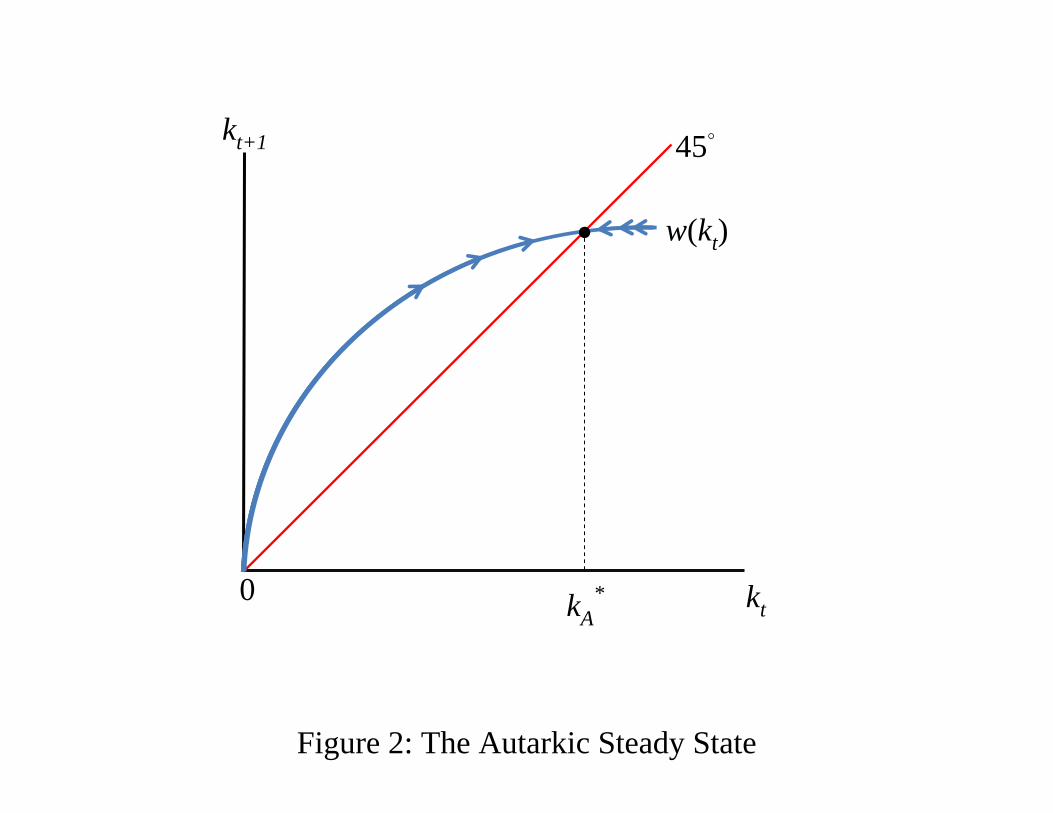
Define x ≡ α(1−α)k̄

wr. Then using (14) and (15), we have

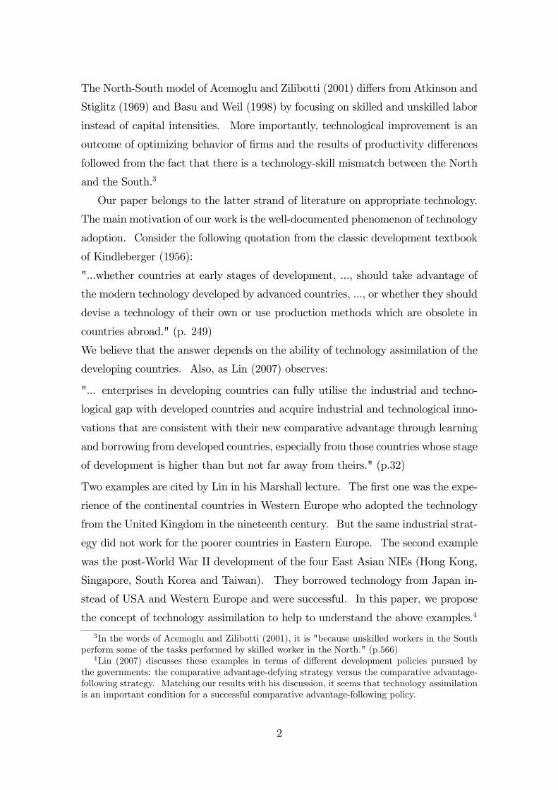
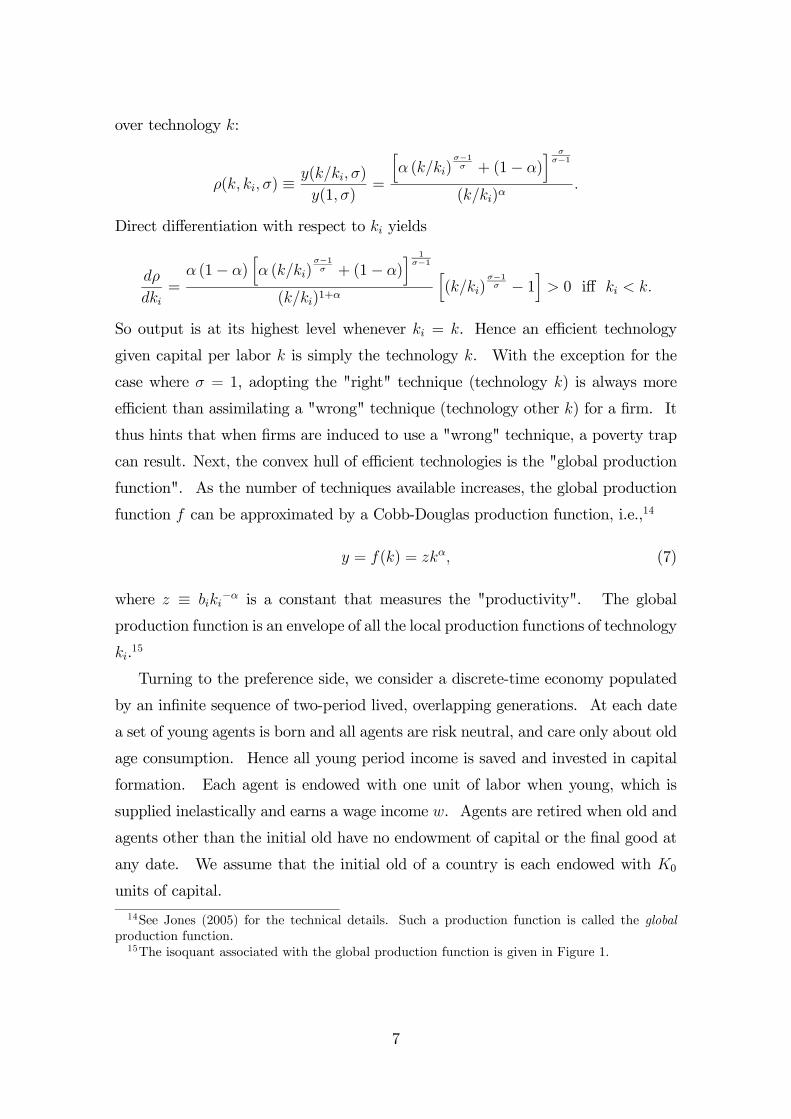
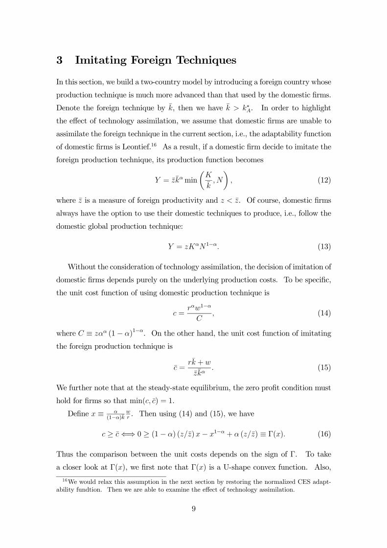
c ≥ c̄⇐⇒ 0 ≥ (1− α) (z/z̄)x− x1−α + α (z/z̄) ≡ Γ(x). (16)

Thus the comparison between the unit costs depends on the sign of Γ. To take

a closer look at Γ(x), we first note that Γ(x) is a U-shape convex function. Also,

16We would relax this assumption in the next section by restoring the normalized CES adapt-ability fundtion. Then we are able to examine the effect of technology assimilation.

9

Γ(0) > 0, Γ(∞) > 0 and Γ(xmin) < 0. So we can conclude that Γ(x) = 0 has two

roots. We provide the graphical representation of Γ(x) in Figure 3. The following

proposition then summarizes our findings of technological imitation.

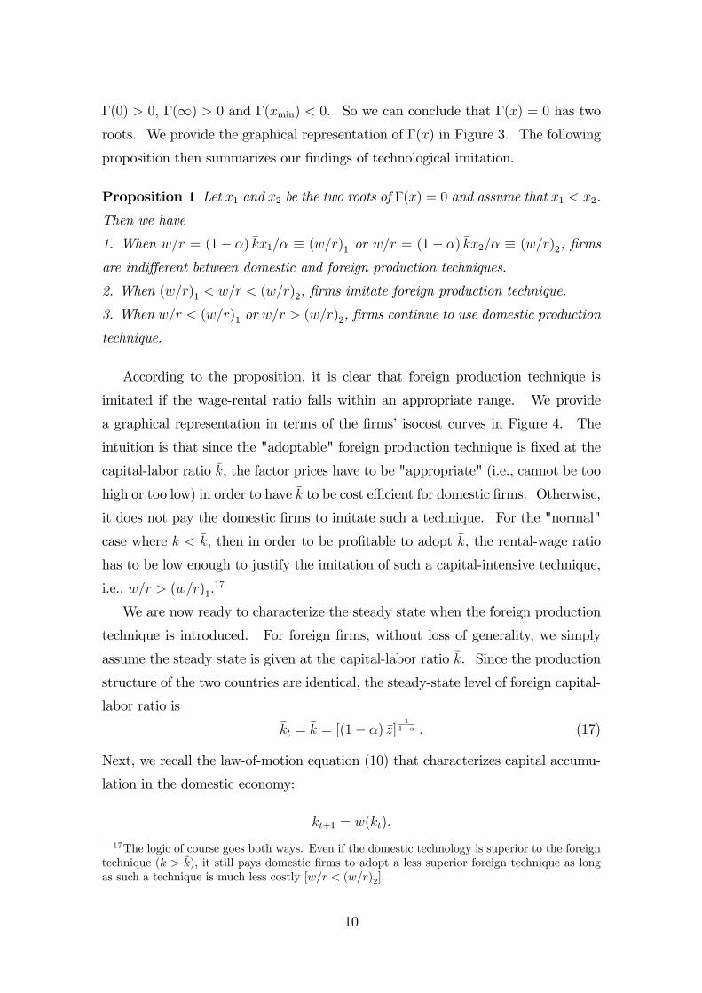
Proposition 1 Let x1 and x2 be the two roots of Γ(x) = 0 and assume that x1 < x2.

Then we have

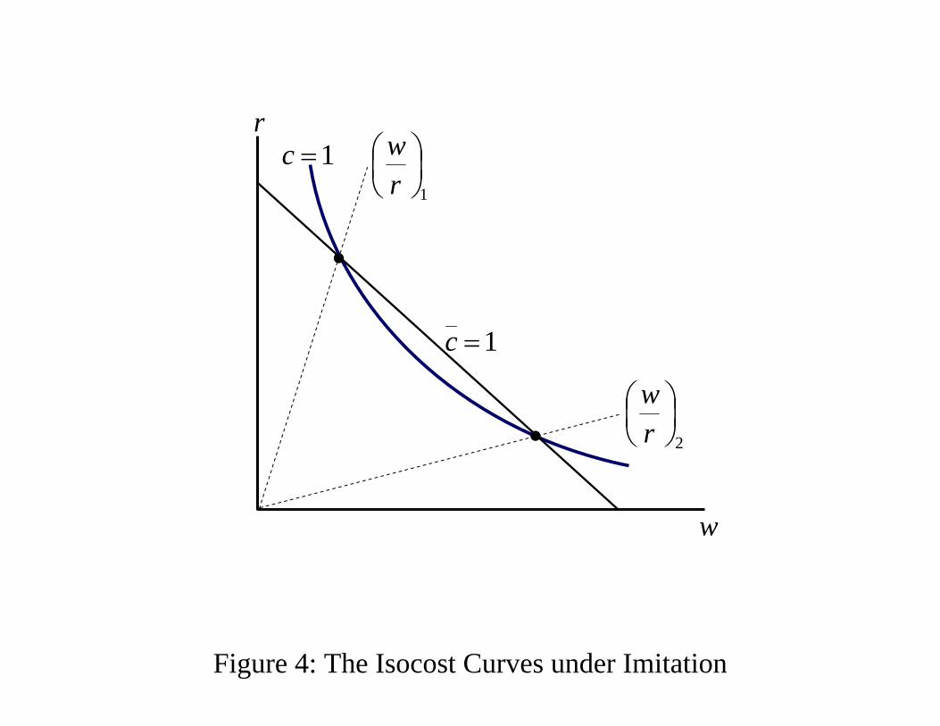
1. When w/r = (1− α) k̄x1/α ≡ (w/r)1 or w/r = (1− α) k̄x2/α ≡ (w/r)2, firmsare indifferent between domestic and foreign production techniques.

2. When (w/r)1 < w/r < (w/r)2, firms imitate foreign production technique.

3. When w/r < (w/r)1 or w/r > (w/r)2, firms continue to use domestic production

technique.

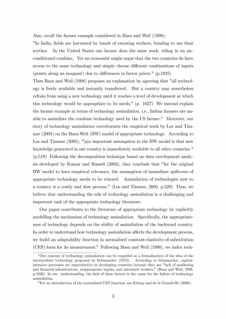
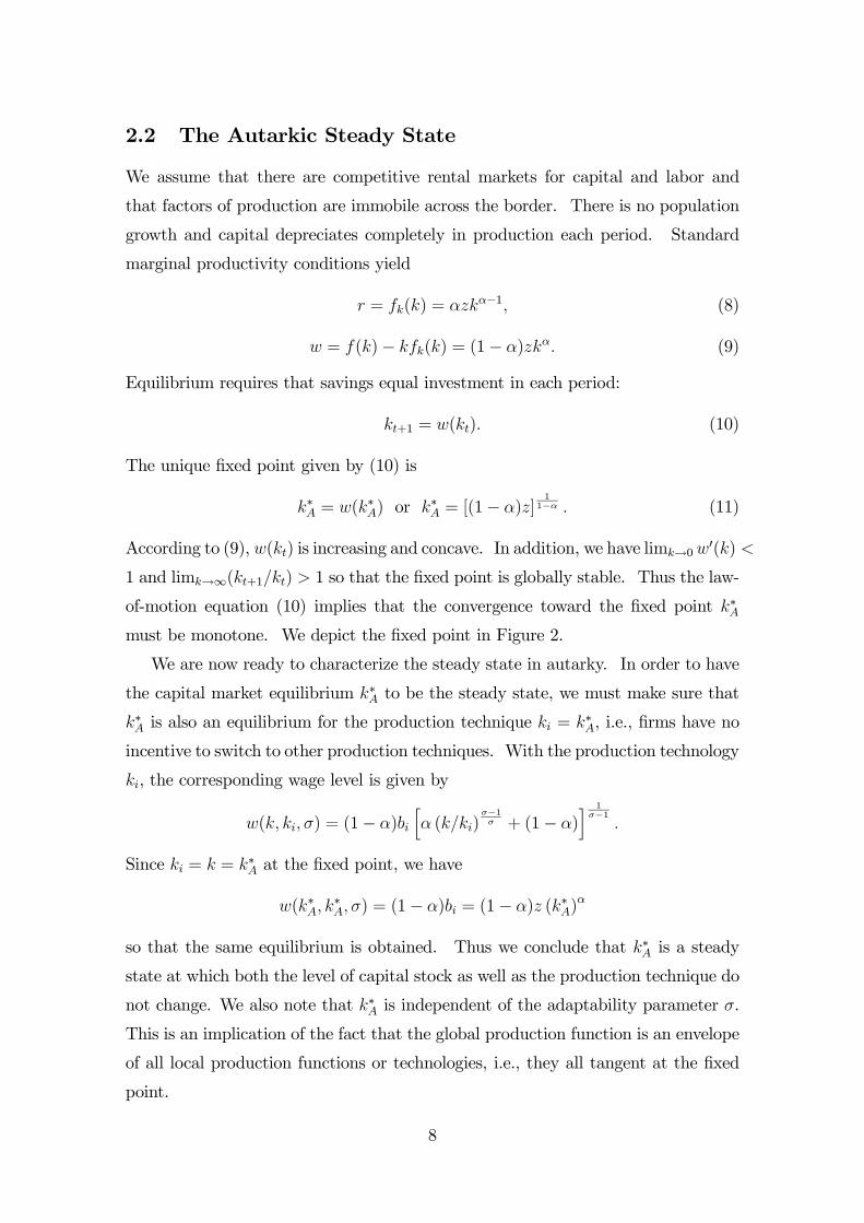
According to the proposition, it is clear that foreign production technique is

imitated if the wage-rental ratio falls within an appropriate range. We provide

a graphical representation in terms of the firms’ isocost curves in Figure 4. The

intuition is that since the "adoptable" foreign production technique is fixed at the

capital-labor ratio k̄, the factor prices have to be "appropriate" (i.e., cannot be too

high or too low) in order to have k̄ to be cost efficient for domestic firms. Otherwise,

it does not pay the domestic firms to imitate such a technique. For the "normal"

case where k < k̄, then in order to be profitable to adopt k̄, the rental-wage ratio

has to be low enough to justify the imitation of such a capital-intensive technique,

i.e., w/r > (w/r)1.17

We are now ready to characterize the steady state when the foreign production

technique is introduced. For foreign firms, without loss of generality, we simply

assume the steady state is given at the capital-labor ratio k̄. Since the production

structure of the two countries are identical, the steady-state level of foreign capital-

labor ratio is

k̄t = k̄ = [(1− α) z̄]1

1−α . (17)

Next, we recall the law-of-motion equation (10) that characterizes capital accumu-

lation in the domestic economy:

kt+1 = w(kt).

17The logic of course goes both ways. Even if the domestic technology is superior to the foreigntechnique (k > k̄), it still pays domestic firms to adopt a less superior foreign technique as longas such a technique is much less costly [w/r < (w/r)2].

10

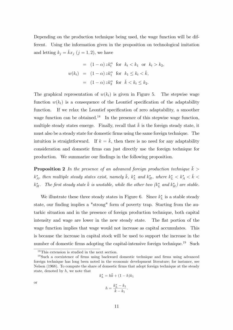
Depending on the production technique being used, the wage function will be dif-

ferent. Using the information given in the proposition on technological imitation

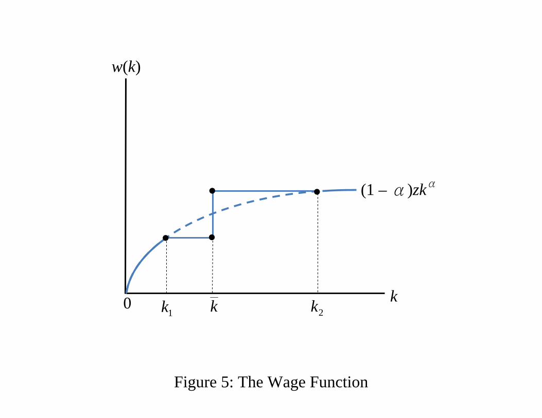
and letting kj = k̄xj (j = 1, 2), we have

= (1− α) zkαt for kt < k1 or kt > k2,

w(kt) = (1− α) zkα1 for k1 ≤ kt < k̄,

= (1− α) zkα2 for k̄ < kt ≤ k2.

The graphical representation of w(kt) is given in Figure 5. The stepwise wage

function w(kt) is a consequence of the Leontief specification of the adaptability

function. If we relax the Leontief specification of zero adaptability, a smoother

wage function can be obtained.18 In the presence of this stepwise wage function,

multiple steady states emerge. Finally, recall that k̄ is the foreign steady state, it

must also be a steady state for domestic firms using the same foreign technique. The

intuition is straightforward. If k = k̄, then there is no need for any adaptability

consideration and domestic firms can just directly use the foreign technique for

production. We summarize our findings in the following proposition.

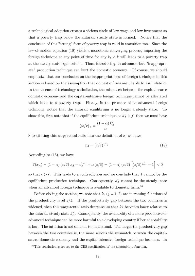
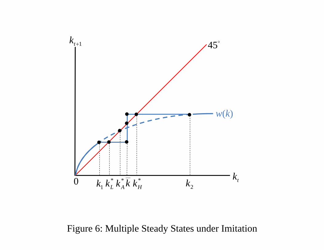
Proposition 2 In the presence of an advanced foreign production technique k̄ >

k∗A, then multiple steady states exist, namely k̄, k∗L and k∗H, where k

∗L < k∗A < k̄ <

k∗H. The first steady state k̄ is unstable, while the other two (k∗L and k

∗H) are stable.

We illustrate these three steady states in Figure 6. Since k∗L is a stable steady

state, our finding implies a "strong" form of poverty trap. Starting from the au-

tarkic situation and in the presence of foreign production technique, both capital

intensity and wage are lower in the new steady state. The flat portion of the

wage function implies that wage would not increase as capital accumulates. This

is because the increase in capital stock will be used to support the increase in the

number of domestic firms adopting the capital-intensive foreign technique.19 Such

18This extension is studied in the next section.19Such a coexistence of firms using backward domestic technique and firms using advanced

foreign technique has long been noted in the economic development literature; for instance, seeNelson (1968). To compute the share of domestic firms that adopt foreign technique at the steadystate, denoted by h, we note that

k∗L = hk̄ + (1− h)k1

or

h =k∗L − k1k̄ − k1

.

11

a technological adoption creates a vicious circle of low wage and low investment so

that a poverty trap below the autarkic steady state is formed. Notice that the

conclusion of this "strong" form of poverty trap is valid in transition too. Since the

law-of-motion equation (10) yields a monotonic converging process, importing the

foreign technique at any point of time for any kt < k̄ will leads to a poverty trap

at the steady-state equilibrium. Thus, introducing an advanced but "inappropri-

ate" production technique can hurt the domestic economy. Of course, we should

emphasize that our conclusion on the inappropriateness of foreign technique in this

section is based on the assumption that domestic firms are unable to assimilate it.

In the absence of technology assimilation, the mismatch between the capital-scarce

domestic economy and the capital-intensive foreign technique cannot be alleviated

which leads to a poverty trap. Finally, in the presence of an advanced foreign

technique, notice that the autarkic equilibrium is no longer a steady state. To

show this, first note that if the equilibrium technique at k∗A is f , then we must have

(w/r)A =(1− α) k∗A

α.

Substituting this wage-rental ratio into the definition of x, we have

xA = (z/z̄)1

1−α . (18)

According to (16), we have

Γ(xA) = (1− α) (z/z̄)xA − x1−αA + α (z/z̄) = (1− α) (z/z̄)h(z/z̄)

11−α − 1

i< 0

so that c > c̄. This leads to a contradiction and we conclude that f cannot be the

equilibrium production technique. Consequently, k∗A cannot be the steady state

when an advanced foreign technique is available to domestic firms.20

Before closing the section, we note that kj (j = 1, 2) are increasing functions of

the productivity level z/z̄. If the productivity gap between the two countries is

widened, then this wage-rental ratio decreases so that k∗L becomes lower relative to

the autarkic steady state k∗A. Consequently, the availability of a more productive or

advanced technique can be more harmful to a developing country if her adaptability

is low. The intuition is not difficult to understand. The larger the productivity gap

between the two countries is, the more serious the mismatch between the capital-

scarce domestic economy and the capital-intensive foreign technique becomes. In20This conclusion is robust to the CES specification of the adaptability function.

12

order to be profitable to imitate a more productive technique, firms must face a

higher return of capital so that wage has to stop growing earlier (or at a lower

level).

4 A Model of Technology Assimilation

In this section, we relax the assumption that domestic firms are unable to assimilate

the foreign technique. Consequently, the effect of technological adoption depends

crucially on the firms’ ability to assimilate the foreign technique. As already

discussed in the autarkic section, we specify the adaptability function for a given

foreign technique k̄ to be a normalized CES function:

Y = z̄k̄αhα¡K/k̄

¢σ−1σ + (1− α)N

σ−1σ

i σσ−1

,

or in per capita terms

y = z̄k̄αhα¡k/k̄

¢σ−1σ + (1− α)

i σσ−1

. (19)

Notice that when the adaptability parameter σ tends to one, we get the foreign

global production function as the assimilation is perfect. Of course, when σ tends

to zero, we get back the Leontief function which is the zero-adaptability case studied

in the previous section.

If firms continue to use domestic production technique, then the unit cost func-

tion remains unchanged:

c =rαw1−α

C,

where C ≡ zαα (1− α)1−α. On the other hand, the unit cost function of adopting

the foreign production technique takes a CES form:

c̄ =

hασ¡rk̄¢1−σ

+ (1− α)σ w1−σi 11−σ

z̄k̄α. (20)

As before, at the steady-state equilibrium, the zero profit condition must hold for

firms so that min(c, c̄) = 1.

Define χ ≡h

α(1−α)k̄

wr

i1−σ. Then using (14) and (20), we have

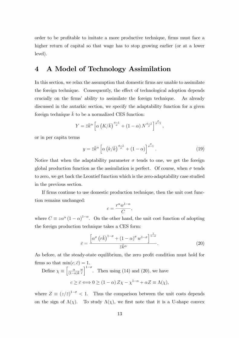
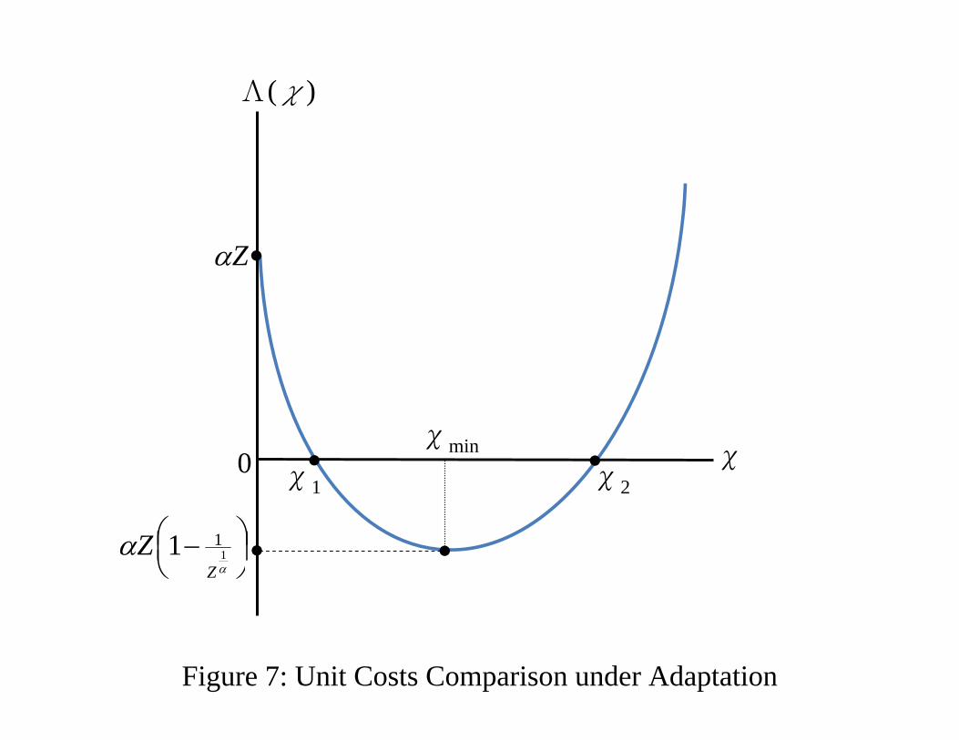
c ≥ c̄⇐⇒ 0 ≥ (1− α)Zχ− χ1−α + αZ ≡ Λ(χ),

where Z ≡ (z/z̄)1−σ < 1. Thus the comparison between the unit costs depends

on the sign of Λ(χ). To study Λ(χ), we first note that it is a U-shape convex

13

function. Also, Λ(0) > 0, Λ(∞) > 0 and Λ(χmin) < 0. So we can conclude that

Λ(χ) = 0 has two roots. We provide the graphical representation of Λ(χ) in Figure

7. The following proposition then summarizes our findings about firms’ choice of

techniques based on unit costs comparison.21

Proposition 3 Let χ1 and χ2 be the two roots of Λ(χ) = 0 and assume that χ1 <

χ2. Then we have

1. When w/r = [(1− α) /α] (χ1)1

1−σ k̄ ≡ (w/r)1 or w/r = [(1− α) /α] (χ2)1

1−σ k̄ ≡(w/r)2, firms are indifferent between domestic and foreign production techniques.

2. When (w/r)1 < w/r < (w/r)2, firms adopt the foreign production technique.

3. When w/r < (w/r)1 or w/r > (w/r)2, firms continue to use the domestic

production technique.

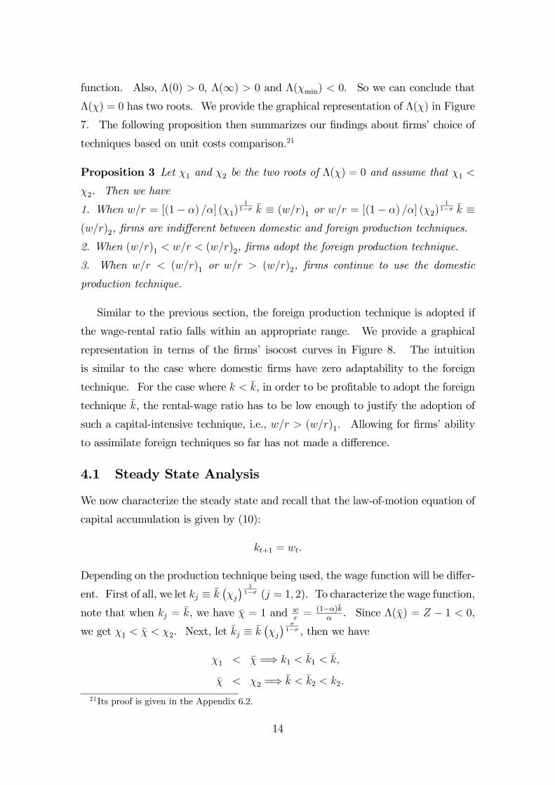
Similar to the previous section, the foreign production technique is adopted if

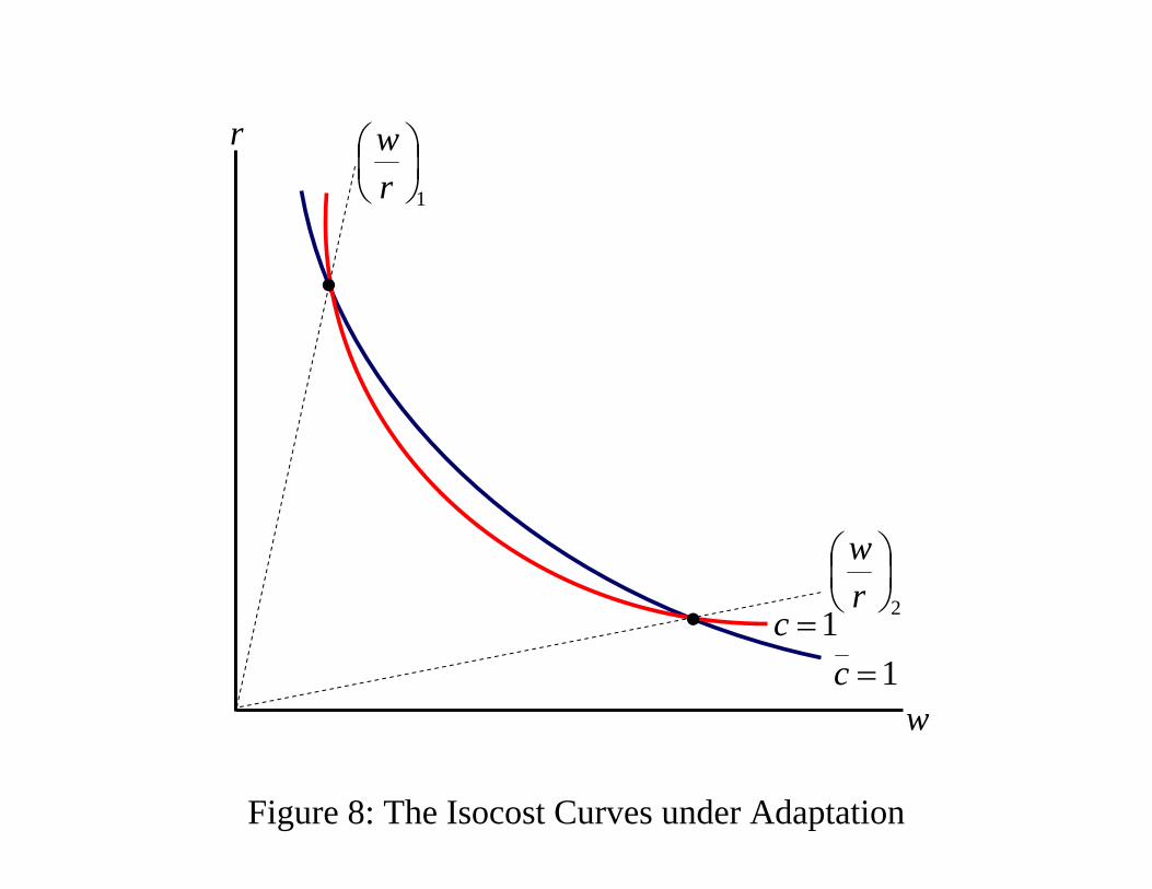
the wage-rental ratio falls within an appropriate range. We provide a graphical

representation in terms of the firms’ isocost curves in Figure 8. The intuition

is similar to the case where domestic firms have zero adaptability to the foreign

technique. For the case where k < k̄, in order to be profitable to adopt the foreign

technique k̄, the rental-wage ratio has to be low enough to justify the adoption of

such a capital-intensive technique, i.e., w/r > (w/r)1. Allowing for firms’ ability

to assimilate foreign techniques so far has not made a difference.

4.1 Steady State Analysis

We now characterize the steady state and recall that the law-of-motion equation of

capital accumulation is given by (10):

kt+1 = wt.

Depending on the production technique being used, the wage function will be differ-

ent. First of all, we let kj ≡ k̄¡χj¢ 11−σ (j = 1, 2). To characterize the wage function,

note that when kj = k̄, we have χ̄ = 1 and wr= (1−α)k̄

α. Since Λ(χ̄) = Z − 1 < 0,

we get χ1 < χ̄ < χ2. Next, let k̄j ≡ k̄¡χj¢ σ1−σ , then we have

χ1 < χ̄ =⇒ k1 < k̄1 < k̄,

χ̄ < χ2 =⇒ k̄ < k̄2 < k2.

21Its proof is given in the Appendix 6.2.

14

Then we can rephrase the above proposition in terms of k instead of the wage-rental

ratio w/r :

Corollary 4 Let kj ≡ k̄¡χj¢ 11−σ (j = 1, 2) and k̄j ≡ k̄

¡χj¢ σ1−σ . Then we have

1. When k1 ≤ k ≤ k̄1 or k̄2 ≤ k ≤ k2, firms are indifferent between domestic and

foreign production techniques.

2. When k̄1 < k < k̄2, firms adopt the foreign technique.

3. When k < k1 or k > k2, firms continue to use the domestic technique.

In the first case of the above corollary, when firms are indifferent between domes-

tic and foreign production techniques, we expect some firms use domestic technique

while others adopt foreign technique. Let h be the share of firms using the foreign

technique f̄ , then we have

k = hk̄j + (1− h)kj or h =k − kjk̄j − kj

(21)

for k being in between kj and k̄j. This then implies that whenever k is in between

kj and k̄j, the wage function is flat since the increase in capital stock will be used to

support the increase in the number of domestic firms adopting the capital-intensive

foreign technique. As a result, wage would not increase as capital accumulates.

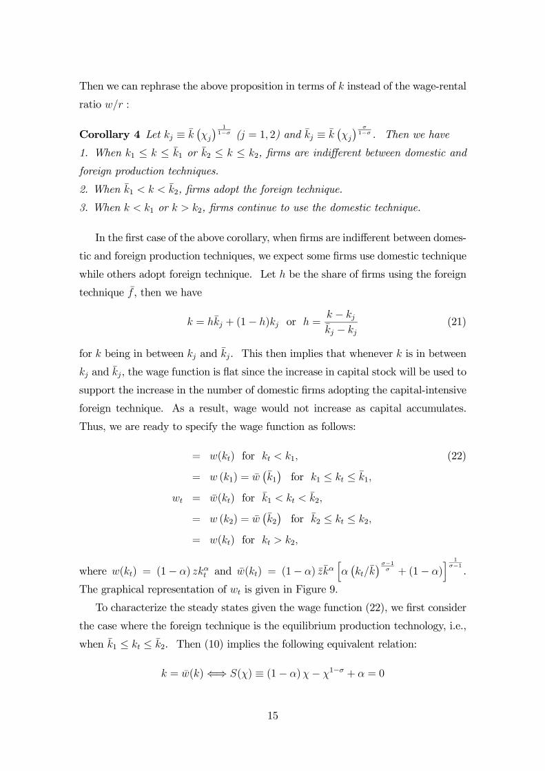
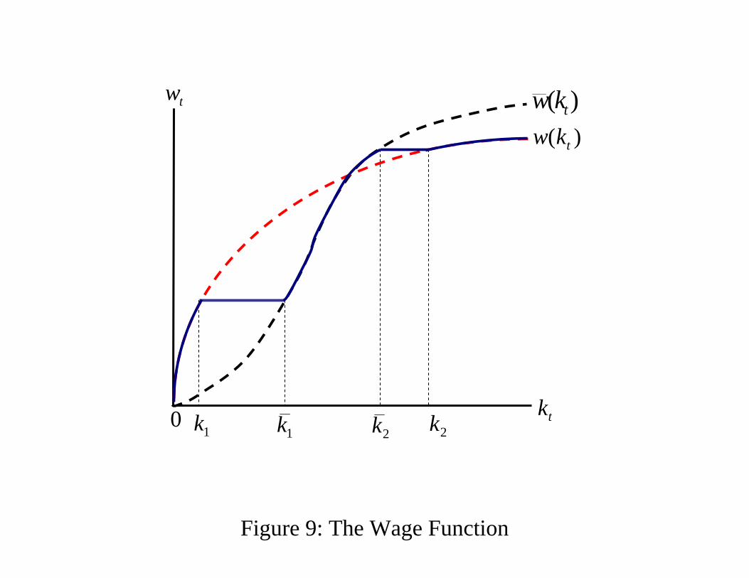
Thus, we are ready to specify the wage function as follows:

= w(kt) for kt < k1, (22)

= w (k1) = w̄¡k̄1¢for k1 ≤ kt ≤ k̄1,

wt = w̄(kt) for k̄1 < kt < k̄2,

= w (k2) = w̄¡k̄2¢for k̄2 ≤ kt ≤ k2,

= w(kt) for kt > k2,

where w(kt) = (1− α) zkαt and w̄(kt) = (1− α) z̄k̄αhα¡kt/k̄

¢σ−1σ + (1− α)

i 1σ−1.

The graphical representation of wt is given in Figure 9.

To characterize the steady states given the wage function (22), we first consider

the case where the foreign technique is the equilibrium production technology, i.e.,

when k̄1 ≤ kt ≤ k̄2. Then (10) implies the following equivalent relation:

k = w̄(k)⇐⇒ S(χ) ≡ (1− α)χ− χ1−σ + α = 0

15

where χ = (k/k̄)(1−σ)/σ.22 Since S00(χ) > 0, S(0) = α and S(∞) =∞, so S(χ) = 0at most have two roots.23 In addition, k = k̄ or χ = 1 is one of the roots and we

denote the other root by k̃. The local stability condition of the roots is given by

w0(k) < 1⇐⇒ S0(χ) > 0. (23)

For k = k̄ or χ = 1, then we have Λ(1) < 0 so that c > c̄. Thus k̄ is a steady

state for the case where f̄ is the equilibrium technique. For the root k = k̃ and

hence χ = χ̃, in order to have f̄ to be the equilibrium technique, we need Λ(χ̃) < 0.

Using the fact that S(χ̃) = 0, we have

Λ(χ̃) = χ̃1−σ¡Z − χ̃σ−α

¢< 0⇐⇒ z

z̄<

Ãk̃

k̄

!1−α/σ. (24)

We summarize our steady-state characterization for the case where f̄ is the equi-

librium technique as follows:

Lemma 5 When f̄ is the equilibrium production technique, then we have at most

two steady states, k̄ and k̃. For the latter to be a steady state, we need zz̄<³

k̃k̄

´1−α/σ. Under dual steady states, if σ > α, then k̄ > k̃ and w0(k̄) < 1 < w0(k̃).

If σ < α, then k̄ < k̃ and w0(k̄) > 1 > w0(k̃).

To avoid being taxonomic, let us focus on the "plausible" case of our steady-

state characterization where k ≤ k̄. For the region where k1 ≤ kt < k̄1, the wage

function is a flat line so at most we have a single steady state. It turns out that the

existence of the steady state in this case depends on (24). Such a steady state, if

it exists, consists of a mix of firms using production techniques f and f̄ . We state

our characterization of the steady state for k1 ≤ kt < k̄1 in the following lemma

with its proof being given in the Appendix 6.3:

Lemma 6 There is a unique steady state, k∗m, in the region£k1, k̄1

¤if and only if

zz̄<³k̃k̄

´1−α/σ.

We are ready to complete our steady state characterization for the general case

of technology assimilation. For kt ≤ k̄, then we have either three steady states

22It is easy to show that χ ≡h

α(1−α)k̄

wr

i1−σ= (k/k̄)(1−σ)/σ.

23For the extreme case of σ = 0 studied in the last section, then k = k̄ or χ = 1 is the only rootof S(χ) = 0. Thus, we have a unique steady state where f̄ is the equilibrium technique.

16

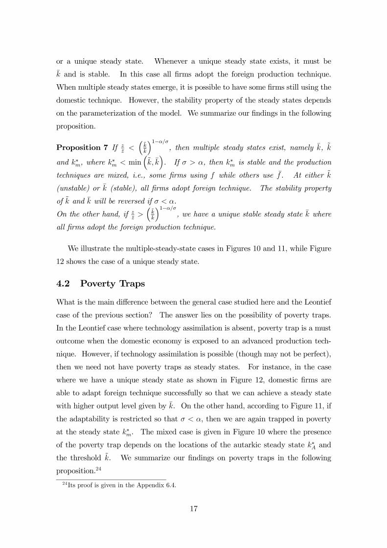
or a unique steady state. Whenever a unique steady state exists, it must be

k̄ and is stable. In this case all firms adopt the foreign production technique.

When multiple steady states emerge, it is possible to have some firms still using the

domestic technique. However, the stability property of the steady states depends

on the parameterization of the model. We summarize our findings in the following

proposition.

Proposition 7 If zz̄<³k̃k̄

´1−α/σ, then multiple steady states exist, namely k̄, k̃

and k∗m, where k∗m < min

³k̃, k̄

´. If σ > α, then k∗m is stable and the production

techniques are mixed, i.e., some firms using f while others use f̄ . At either k̃

(unstable) or k̄ (stable), all firms adopt foreign technique. The stability property

of k̃ and k̄ will be reversed if σ < α.

On the other hand, if zz̄>³k̃k̄

´1−α/σ, we have a unique stable steady state k̄ where

all firms adopt the foreign production technique.

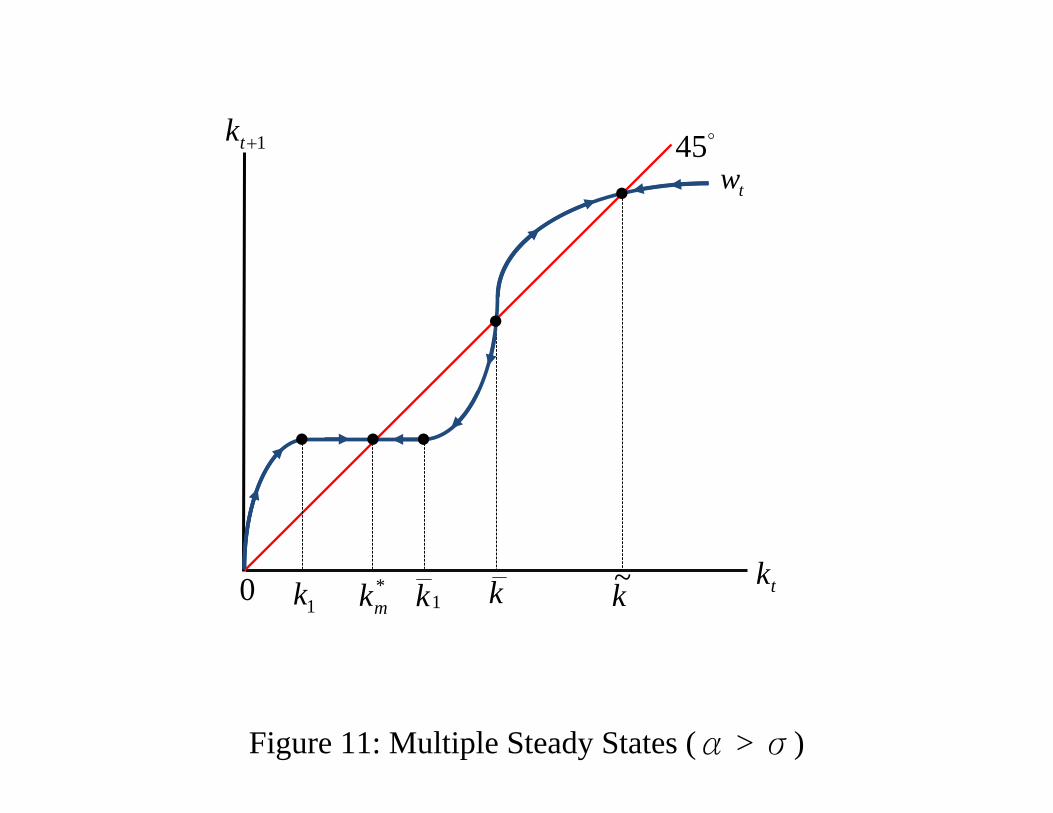
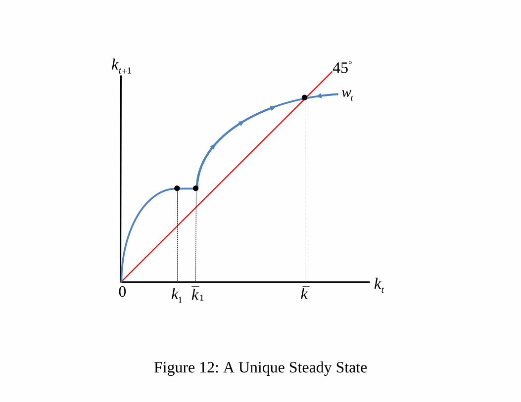
We illustrate the multiple-steady-state cases in Figures 10 and 11, while Figure

12 shows the case of a unique steady state.

4.2 Poverty Traps

What is the main difference between the general case studied here and the Leontief

case of the previous section? The answer lies on the possibility of poverty traps.

In the Leontief case where technology assimilation is absent, poverty trap is a must

outcome when the domestic economy is exposed to an advanced production tech-

nique. However, if technology assimilation is possible (though may not be perfect),

then we need not have poverty traps as steady states. For instance, in the case

where we have a unique steady state as shown in Figure 12, domestic firms are

able to adapt foreign technique successfully so that we can achieve a steady state

with higher output level given by k̄. On the other hand, according to Figure 11, if

the adaptability is restricted so that σ < α, then we are again trapped in poverty

at the steady state k∗m. The mixed case is given in Figure 10 where the presence

of the poverty trap depends on the locations of the autarkic steady state k∗A and

the threshold k̃. We summarize our findings on poverty traps in the following

proposition.24

24Its proof is given in the Appendix 6.4.

17

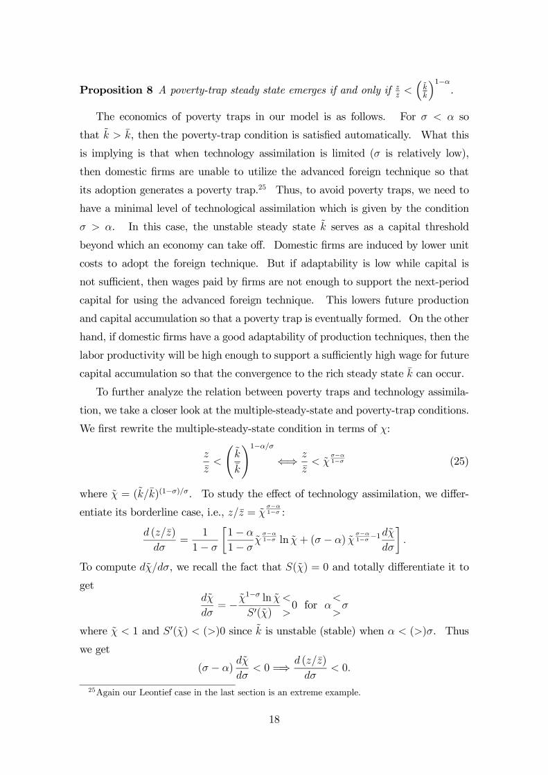
Proposition 8 A poverty-trap steady state emerges if and only if zz̄<³k̃k̄

´1−α.

The economics of poverty traps in our model is as follows. For σ < α so

that k̃ > k̄, then the poverty-trap condition is satisfied automatically. What this

is implying is that when technology assimilation is limited (σ is relatively low),

then domestic firms are unable to utilize the advanced foreign technique so that

its adoption generates a poverty trap.25 Thus, to avoid poverty traps, we need to

have a minimal level of technological assimilation which is given by the condition

σ > α. In this case, the unstable steady state k̃ serves as a capital threshold

beyond which an economy can take off. Domestic firms are induced by lower unit

costs to adopt the foreign technique. But if adaptability is low while capital is

not sufficient, then wages paid by firms are not enough to support the next-period

capital for using the advanced foreign technique. This lowers future production

and capital accumulation so that a poverty trap is eventually formed. On the other

hand, if domestic firms have a good adaptability of production techniques, then the

labor productivity will be high enough to support a sufficiently high wage for future

capital accumulation so that the convergence to the rich steady state k̄ can occur.

To further analyze the relation between poverty traps and technology assimila-

tion, we take a closer look at the multiple-steady-state and poverty-trap conditions.

We first rewrite the multiple-steady-state condition in terms of χ:

z

z̄<

Ãk̃

k̄

!1−α/σ⇐⇒ z

z̄< χ̃

σ−α1−σ (25)

where χ̃ = (k̃/k̄)(1−σ)/σ. To study the effect of technology assimilation, we differ-

entiate its borderline case, i.e., z/z̄ = χ̃σ−α1−σ :

d (z/z̄)

dσ=

1

1− σ

∙1− α

1− σχ̃

σ−α1−σ ln χ̃+ (σ − α) χ̃

σ−α1−σ −1

dχ̃

dσ

¸.

To compute dχ̃/dσ, we recall the fact that S(χ̃) = 0 and totally differentiate it to

getdχ̃

dσ= − χ̃

1−σ ln χ̃

S0(χ̃)

<

>0 for α

<

>σ

where χ̃ < 1 and S0(χ̃) < (>)0 since k̃ is unstable (stable) when α < (>)σ. Thus

we get

(σ − α)dχ̃

dσ< 0 =⇒ d (z/z̄)

dσ< 0.

25Again our Leontief case in the last section is an extreme example.

18

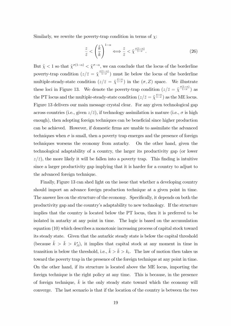
Similarly, we rewrite the poverty-trap condition in terms of χ:

z

z̄<

Ãk̃

k̄

!1−α⇐⇒ z

z̄< χ̃

σ(1−α)1−σ . (26)

But χ̃ < 1 so that χ̃σ(1−α) < χ̃σ−α, we can conclude that the locus of the borderline

poverty-trap condition (z/z̄ = χ̃σ(1−α)1−σ ) must lie below the locus of the borderline

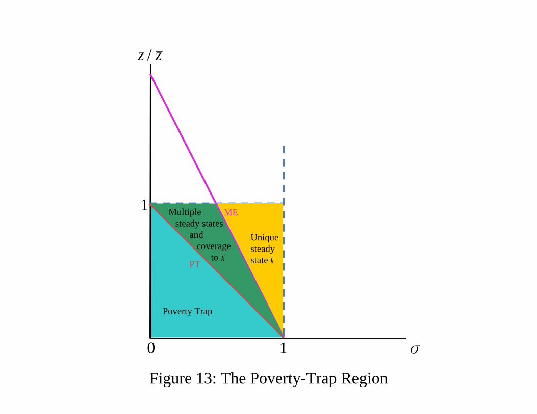
multiple-steady-state condition (z/z̄ = χ̃σ−α1−σ ) in the (σ,Z) space. We illustrate

these loci in Figure 13. We denote the poverty-trap condition (z/z̄ = χ̃σ(1−α)1−σ ) as

the PT locus and the multiple-steady-state condition (z/z̄ = χ̃σ−α1−σ ) as the ME locus.

Figure 13 delivers our main message crystal clear. For any given technological gap

across countries (i.e., given z/z̄), if technology assimilation is mature (i.e., σ is high

enough), then adopting foreign techniques can be beneficial since higher production

can be achieved. However, if domestic firms are unable to assimilate the advanced

techniques when σ is small, then a poverty trap emerges and the presence of foreign

techniques worsens the economy from autarky. On the other hand, given the

technological adaptability of a country, the larger its productivity gap (or lower

z/z̄), the more likely it will be fallen into a poverty trap. This finding is intuitive

since a larger productivity gap implying that it is harder for a country to adjust to

the advanced foreign technique.

Finally, Figure 13 can shed light on the issue that whether a developing country

should import an advance foreign production technique at a given point in time.

The answer lies on the structure of the economy. Specifically, it depends on both the

productivity gap and the country’s adaptability to new technology. If the structure

implies that the country is located below the PT locus, then it is preferred to be

isolated in autarky at any point in time. The logic is based on the accumulation

equation (10) which describes a monotonic increasing process of capital stock toward

its steady state. Given that the autarkic steady state is below the capital threshold

(because k̃ > k̄ > k∗A), it implies that capital stock at any moment in time in

transition is below the threshold, i.e., k̃ > k̄ > kt. The law of motion then takes us

toward the poverty trap in the presence of the foreign technique at any point in time.

On the other hand, if its structure is located above the ME locus, importing the

foreign technique is the right policy at any time. This is because, in the presence

of foreign technique, k̄ is the only steady state toward which the economy will

converge. The last scenario is that if the location of the country is between the two

19

loci in Figure 13, then the timing of importing an advance production technique is

important. If the country is already in its autarkic steady state, then it converges

toward the "rich" steady state k̄ so that opening is the right choice. But this

conclusion does not hold for all time in transition. It is possible that at time τ

when the foreign technique is introduced, we have k∗A > k̃ > kτ so that the capital

threshold has not been reached. If this is the case, then the economy will converge

toward the poverty trap despite the fact that we have k̃ < k∗A. This implies that

there exists a time threshold for capital accumulation in transition beyond which

would make opening the right policy to follow. Opening too early would not be a

good matter which gives us an "infant-industry" favor from the trade literature.

5 Concluding Remarks

This paper studies the mechanism of technology assimilation and examines its effects

on economic development. In the absence of technology assimilation, imitating

an advanced foreign technology is inappropriate in the sense that the backward

country will achieve a steady state where both its capital intensity and wage are

lower than in autarky. This is due to the fact that the increase in capital from

higher production is directed to support the increase in the number of domestic

firms adopting the new capital-intensive technique so that a vicious cycle of low

wage and low investment is created. This then leads to a poverty trap below the

autarkic steady state. However, if technology assimilation is allowed, then adopting

an advance foreign technology can be a successful policy for development. We find

that the key to successful technology adoption is a country’s ability to technology

assimilation. Using a CES adaptability function where the degree of technology

assimilation is measured by the elasticity of substitution, we provide a condition in

terms of a minimum level of the elasticity so as to avoid poverty traps in technology

adoption. The main message is that if technology assimilation is not mature (given

by a lower elasticity of substitution of the CES adaptability function), then wages

are not sufficient to support capital for the advanced technology. As a result, future

production declines and a poverty trap is formed.

Given the North-South technological gap, if the South’s ability to technology

assimilation is good, then converging to the steady state equilibrium of the North is

almost a sure outcome through technology adoption. For a lower ability of assim-

20

ilation where multiple steady states emerge, then economic development through

technology adoption requires a minimum level of capital. Finally, if the ability

of assimilation is poor, then imitating foreign technology leads to a poverty trap.

The policy implication from our paper is clear. If the ability of technology as-

similation of a country is not strong, then a big-push type of development policy

is called for so as to make sure that the country has enough capital to start off.

If technology assimilation is almost absent, then conventional policies like the big

push or subsidizing R&D for technology adoption may be futile which is in contrast

to the existing literature of economic development. For instance, Rustichini and

Schmitz (1991) argue that imitation plays an important role to developing countries

so that it is optimal to subsidize imitation in their model. Our paper provides an

alternative mechanism to generate a different result.26 We emphasize that whether

imitation can be successful depends crucially on a country’s ability of technology

assimilation.26The conventional wisdom of subsidizing technology-advancing activities has also been chal-

lenged by others. For example, from the perspective of political economy, Boldrin and Levine(2004) show that policies of forstering innovations and their adoption like patents may not beoptimal due to rent-seeking behavior of the private and public sectors.

21

6 Appendix

6.1 The Derivation of the Adaptability Function

Following Klump and de la Grandville (2000), we first specify the three arbitrarily

chosen baseline variables of the normalized CES function: a capital-labor ratio ki,

the per capita production yi = f(ki) = zki, and the marginal rate of substitution

mi = [f(ki)− kif0(ki)] /f

0(ki) = (1− α) ki/α. The normalized capital-labor ratio

will be taken to be the production technique ki that being assimilated. As a result,

the family of the normalized CES functions mimics the family of the adaptability

functions ordered by their ability to assimilate advanced production techniques. In

summary, the normalized CES function becomes

f(k, σ) = A (σ)ha (σ) (k/ki)

σ−1σ + (1− a (σ))

i σσ−1

(27)

where

A (σ) = yi

"k1/σi +mi

ki +mi

# σσ−1

, (28)

a (σ) =k1/σi

k1/σi +mi

. (29)

Substituting (28) and (29) into (27), we get

f(k, σ) = Ahα (k/ki)

σ−1σ + (1− α)

i σσ−1

where A = yi. This is the per capita adaptability function q(k/ki, σ) given by (6)

in the text.

6.2 Proof of Proposition 3

Since χ1 and χ2 are the two roots of Λ(χ) = 0 and χ1 < χ2, we have

1. When χ < χ1 or χ > χ2, firms continue to use domestic production technique

because c < c̄.

2. When χ1 < χ < χ2, firms adopt foreign production technique because c > c̄.

3. When χ = χ1 or χ = χ2, firms are indifferent between domestic and foreign

production techniques because c = c̄.

Using the definition of χ and rewrite the above findings in terms of w/r, the results

follow.

22

6.3 Proof of Lemma 6

In the region of£k1, k̄1

¤, if the steady state exists, then the wage function has to

satisfy the following inequalities:

k1 ≤ w (k1) = w̄¡k̄1¢≤ k̄1. (30)

The first inequality can be rewritten as

k1 ≤ (1− α) zkα1 or k1 ≤ [(1− α) z]1/(1−α) = k∗A.

But we have already shown that in the presence of f̄ no firms will be using f in the

autarkic steady state. But k1 is the maximum level of k when firms are using f ,

thus we must have k∗A > k1. For the second inequality, we get

w̄¡k̄1¢≤ k̄1 ⇐⇒ S(χ(k̄1)) ≥ 0. (31)

Now recall (24). If it holds, then both k̄ and k̃ are steady states for k̄1 < kt < k̄2.

So we have min³k̄, k̃

´> k̄1 or min

hχ¡k̄¢, χ³k̃´i

> χ¡k̄1¢. Recall that S(χ)

is U-shaped and S(χ¡k̄¢) = S

³χ³k̃´´

= 0, we get S¡χ¡k̄1¢¢

> 0 and (30) is

satisfied.

If (24) does not hold, then only k̄ is the steady state for k̄1 < kt < k̄2. Since

f̄ is not the equilibrium technique at k = k̃, we then have k̄ > k̄1 > k̃ and hence

S¡χ¡k̄1¢¢

< 0. The inequality (31) is violated and so there is no steady state in

the region of£k1, k̄1

¤.

Likewise, using the same procedure, we can show that for the range£k̄2, k2

¤, if

(24) holds, we get a unique steady state. Otherwise, no steady state exists when

(24) fails.

6.4 Proof of Proposition 8

It is easy to see that a poverty trap emerges when k∗A < min³k̃, k̄

´. For k̃ > k̄,

then we must have k̃ > k̄ > k∗A since k̄ is the foreign steady state. For the case

where k̃ < k̄, then k̃ is unstable so that poverty traps require k̃ > k∗A. But it is

easy to show that k̃ > k∗A ⇐⇒ zz̄<³k̃k̄

´1−αand the result follows.

23

References

[1] Acemoglu, D., Zilibotti, F., 2001. Productivity differences. Quarterly Journal

of Economics 116 (2), 563-606.

[2] Atkinson, A., Stiglitz, J., 1969. A new view of technological change. Economic

Journal 79, 573-578.

[3] Barro, R., Sala-i-Martin, X., 1997. Technological diffusion, convergence, and

growth. Journal of Economic Growth 2, 1-26.

[4] Basu, S., Weil, D., 1998. Appropriate technology and growth. Quarterly Jour-

nal of Economics 113, 1025-1054.

[5] Boldrin, M., Levine, D., 2004. Rent-seeking and innovation. Journal of Mone-

tary Economics 51, 127-160.

[6] Caselli, F., Coleman, W., 2006. The world technology frontier. American Eco-

nomic Review 96 (3), 499-522.

[7] Chen, B., Mo, J., Wang, P., 2002. Market frictions, technology adoption and

economic growth. Journal of Economic Dynamics & Control 26, 1927-1954.

[8] Grossman, G., Helpman, E., 1991. Innovation and growth in the global econ-

omy. MIT Press, Cambridge, MA.

[9] Hall, R., Jones, C., 1999. Why do some countries produce so much more output

per worker than others? Quarterly Journal of Economics 114, 83-116.

[10] Jones, C., 2005. The shape of production functions and the direction of tech-

nical change. Quarterly Journal of Economics 120 (2), 517-549.

[11] Kindleberger, C., 1956. Economic development. McGraw Hill, New York.

[12] Klump, R., de la Grandville, O., 2000. Economic growth and the elasticity of

substitution: two theorems and some suggestions. American Economic Review

90, 282-291.

[13] Kumar, S., Russell, R., 2002. Technological change, technological catch-up, and

capital deepening: relative contributions to growth and convergence. American

Economic Review 92, 66-83.

24

[14] Lin, J., 2007. Development and transition: idea, strategy, and viability. The

Marshall Lectures, Cambridge University, England.

[15] Los, B., Timmer, M., 2005. The ’appropriate technology’ explanation of pro-

ductivity growth differentials: An empirical approach. Journal of Development

Economics 77, 517-531.

[16] Nelson, R., 1968. A diffusion model of international productivity differences.

American Economic Review 58, 1219-1248.

[17] Parente, S., Prescott, E., 1994. Barriers to technology adoption and develop-

ment. Journal of Political Economy 102 (2), 298-321.

[18] Parente, S., Prescott, E., 1999. Monopoly rights: a barrier to riches. American

Economic Review 89 (5), 1216-1233.

[19] Prescott, E., 1998. Needed: a theory of total factor productivity. International

Economic Review 39, 525-553.

[20] Rustichini, A., Schmitz, J., 1991. Research and imitation in long-run growth.

Journal of Monetary Economics 27 (2), 271-292.

[21] Schumacher, E., 1973. Small is beautiful: economics as if people mattered. New

York, NY: Harper and Row.

[22] Segerstrom, P., Anant, T., Dinapoulos, E., 1990. A Schumpeterian model of

the product life cycle. American Economic Review 80, 1077-1092.

[23] Wang, P., Xie, D., 2004. Activation of a modern industry. Journal of Develop-

ment Economics 74, 393-410.

25

production techniques (σ < 0)

production technology (σ < 1)

production function (σ = 1)

K

N0

Figure 1: The Production Concepts

•

•

kt+1

0 kt

w(kt)

45°

kA*

•

Figure 2: The Autarkic Steady State

Γ(x)

x0 • ••x1 x2xmin

Figure 3: Unit Costs Comparison under Imitation

r

w

•

•

1⎟⎠⎞

⎜⎝⎛

rw

2⎟⎠⎞

⎜⎝⎛

rw

1=c

1=c

Figure 4: The Isocost Curves under Imitation

0

w(k)

(1 – α)zkα

k1k

Figure 5: The Wage Function

•

•

•

•

2k k

0

w(k)

k1k 2k

Figure 6: Multiple Steady States under Imitation

•

•

••

••

•

•

*Lk *

Ak *Hk

1+tk

tk

45°

Λ(χ)

χ0 • •

•

χ1 χ2

•Zα

⎟⎠⎞⎜

⎝⎛ −

αα 1

11Z

Z •

Figure 7: Unit Costs Comparison under Adaptation

χmin

2⎟⎠⎞

⎜⎝⎛

rw

1⎟⎠⎞

⎜⎝⎛

rwr

w1=c

1=c

•

•

Figure 8: The Isocost Curves under Adaptation

tw

tk01k 2k1k

)( tkw

2k

Figure 9: The Wage Function

)( tkw

0 1k1k k

45°

k~*mk tk

1+tk

Figure 10: Multiple Steady States (σ > α)

tw

• •

•

•

•

0

45°

tk

1+tk

Figure 11: Multiple Steady States (α > σ)

• •

•

•

•

1k1k k k~*mk

tw

01k k

45°

tk

1+tk

Figure 12: A Unique Steady State

1k

tw

•

•

•

0

zz /

Figure 13: The Poverty-Trap Region

1 σ

1

Poverty Trap

PTk

Multiplesteady states

andcoverage

to

ME

Unique steady state k