1

SIXTH FRAMEWORK PROGRAMME

Project no: 502687 NEEDS

New Energy Externalities Developments for Sustainability

INTEGRATED PROJECT Priority 6.1: Sustainable Energy Systems and, more specifically,

Sub-priority 6.1.3.2.5: Socio-economic tools and concepts for energy strategy.

Technical paper n° 4.1 - RS Ia

“Development of parameterisation methods to derive transferable life cycle inventories”

Technical guideline on parameterisation of life cycle inventory data

Due date of paper: Actual submission date: 28.02.2009 Start date of project: 1 September 2004 Duration: 48 months Organisation name for this paper: PSI Authors: Thomas Heck, Christian Bauer, Roberto Dones. (With contributions from Sven Gärtner, Peter Viebahn, Oliver Mayer-Spohn, Markus Blesl).

Project co-funded by the European Commission within the Sixth Framework Programme Dissemination Level

PU Public X PP Restricted to other programme participants (including the Commission Services) RE Restricted to a group specified by the consortium (including the Commission

Services)

CO Confidential, only for members of the consortium (including the Commission Services)

2

Contents Summary .................................................................................................................................... 4 1 Introduction ........................................................................................................................ 5 2 Why parameterisation of LCA ? ........................................................................................ 5 3 Parameterisation of LCA data - General framework ......................................................... 8 4 Examples of time-, technology-, and space-dependent parameters ................................. 11

4.1 Time-dependency ..................................................................................................... 11 4.2 Technology-dependency .......................................................................................... 16 4.3 Space-dependency.................................................................................................... 20 4.4 External costs results example ................................................................................. 24

5 Selected parameters of electricity generation systems ..................................................... 27 5.1 Advanced fossil ........................................................................................................ 27 5.2 Bioenergy ................................................................................................................. 39 5.3 Photovoltaics ............................................................................................................ 43 5.4 Solar thermal power ................................................................................................. 45 5.5 Wind ......................................................................................................................... 48 5.6 Hydrogen.................................................................................................................. 49 5.7 Fuel cells .................................................................................................................. 49 5.8 Nuclear ..................................................................................................................... 50 5.9 Wave and tidal power............................................................................................... 50 5.10 Hydropower.............................................................................................................. 50

6 Conclusions ...................................................................................................................... 52 7 References ........................................................................................................................ 53

3

Abbreviations BOP Balance of plants CC Combined Cycle CCS Carbon Capture and Storage CHP Combined Heat and Power DNI Direct Normal Irradiation ECLIPSE Environmental and eCological Life cycle Inventories for present and future

Power Systems in Europe EIA Environmental Impact Assessment GCC Gas Combined Cycle GHG Greenhouse Gas GIS Geographical Information System IGCC Integrated Gasification Combined Cycle IPCC Intergovernmental Panel on Climate Change kWh kilo Watt hour kWhe kilo Watt hour electricity LCA Life Cycle Assessment LCI Life Cycle Inventory LCIA Life Cycle Impact Assessment LEC Levelised Electricity Costs LHV Lower Heating Value LRV Luftreinhalteverordnung NEEDS New Energy Externalities Developments for Sustainability NG Natural Gas NMVOC Non-methane Volatile Organic Compounds PAH Polycyclic aromatic hydrocarbons PM Particulate Matter PM10 Particulate Matter with diameter up to 10 micro-metre ppm parts per million PV Photovoltaics

4

Summary

Traditionally, life cycle analyses and life cycle impact analyses do not consider space- and time-dependencies. In reality, the environmental performance of energy technologies may vary in space and time, while their main characteristics remain the same. The objective of this work package was the outline of a parameterisation method that facilitates the description of space- and time-dependent life cycle data for energy systems. In the LCA part of the NEEDS project, the future development of electricity generation technologies and LCA background processes up to the year 2050 has been assessed. The coverage of a broad spectrum of future technologies and a long time scale based on the framework of the large ecoinvent database is a substantial achievement for life cycle assessment of energy systems. The present technical report provides some new ideas and proposes new methodologies on parameterisation of LCA modelling that are intended to support further extensions of space and time coverage beyond what has been achieved already within the NEEDS LCA modelling. The intention is also to contribute to the improvement of assessment of space- and time-dependent impact and external cost effects in connection with LCI data. Environmental impacts and external costs depend a lot on site-specific conditions. Therefore a higher spatial differentiation of LCI modelling compared to current models is desirable. Firstly, general aspects of an advanced parameterised LCA system are discussed. It is proposed that the connection of the LCA model to a Geographical Information System (GIS) should be considered because several spatial parameters can be treated systematically in a GIS software. A couple of explicit examples of parameters relevant for energy systems under the perspective of space-dependency, time-dependency and technology-dependency that could be implemented into an advanced LCA system are provided. For a number of advanced electricity generation technologies, overviews on important space- and time-dependent parameters are given. The coverage and depth of the discussion varies for the different energy systems according to the estimated practicability and relevance for LCA. Parameters provided within the NEEDS project for the different technologies are also considered where appropriate. Generally, it can be concluded that the possibility and appropriateness of parameterisation depends much on the specific energy system, in particular for the space-dependency. The focus of the present work was more on the variety of parameters that have to be considered rather than completeness. The implementation of the proposed methods up to a running advanced LCA model would require deeper investigations of the variety of energy systems and background processes and would need substantial resources. The implementation can proceed in an iterative way because already a partial parameterisation can be advantageous for further extensions of LCA models and databases in view of the large number of parameters in present LCA modelling.

5

1 Introduction

The environmental performance of energy technologies may vary in space and time, while their main characteristics remain the same. The objective of this work package was the outline of a parameterisation method that facilitates the description of space- and time-dependent life cycle data for energy systems. Results are intended to support the efficient specification of region- and time-specific LCI datasets in reasonable resolution. This will improve the possibilities to assess space- and time-dependent impact and external cost effects.

2 Why parameterisation of LCA ?

The Life Cycle Assessment (LCA) part of the NEEDS project (stream RS1a) has been based on the ecoinvent database (www.ecoinvent.com). Ecoinvent is probably the most comprehensive life cycle inventory (LCI) worldwide. It includes inventory data on energy supply, material supply, transport services, chemicals, metals, agriculture, waste management services, and resource extraction. The environmental part of the database includes emissions to air, to water, and to soil as well as land use and resources taken from nature.

Technically, the ecoinvent database has essentially the structure shown in Fig. 2.1. The different research groups contribute input to three types of data which are then organised in three matrices. Firstly, the input process matrix (sometimes called “technosphere matrix”) links a process to other processes of the technosphere. The technosphere processes refer to energy systems, chemicals, transport, agriculture, etc. Secondly, the elementary flow matrix (sometimes called “biosphere matrix”) describes the use of resources from nature and the emissions to nature for each process. Finally, a set of impact assessment and valuation methods is included in the LCIA (life cycle impact assessment) matrix. For the LCA stream in the NEEDS project, mainly external costs have been discussed. The major outputs for the users are the cumulative LCI results which include the direct and indirect flows from and to nature for each process and the cumulative LCIA results for each process.

The input and output of the database uses the so-called “EcoSpold” format (see www.ecoinvent.com). The definition of the EcoSpold format during the development of ecoinvent was a big breakthrough for the communication of LCI data between different software products. As a consequence, the ecoinvent data has been included in many LCA software packages (Umberto, GaBi, Regis, EMIS, Green-e, Bilan Produit, WRATE, SimaPro) in order to serve as a basis for subsequent LCA studies.

6

Fig. 2.1 Basic structure of the current ecoinvent LCI and LCIA database (m = number of processes, n = number of flows to and from nature, r = number of LCIA methods).

The advantage of the relatively simple data scheme is that different research groups can quickly set up new LCA data in the EcoSpold format and combine knowledge from different research fields.

Nevertheless, as it is, the organisation of large datasets has also disadvantages as one can see from the mere number of entries included in the database. Tab. 2.1 shows the number of input entries for the LCI part of ecoinvent version 1.1 which was the starting point of the NEEDS project. The database comprised already more than 65’000 entries which are formally treated as independent parameters for the calculation of cumulative results. Additionally, the LCI database is supplemented by about 200 LCIA methods (on the subcategory level). NEEDS and other projects further extend the number of processes and entries. Furthermore, different time series for future scenarios have been investigated in the NEEDS project.

Tab. 2.1 Size of the LCI part of the ecoinvent database (v 1.1)

number of processes and flows number of entries (parameters)

input process matrix about 2600 processes about 23’500

elementary flow matrix about 1000 flows about 42’000

total LCI input about 65’500

The increasing complexity of the databases is difficult to handle. Moreover, extending the datasets in space and time, while keeping control over consistency and correctness, becomes more and more difficult.

Among the huge number of input parameters, not all are really independent, and not all are really relevant with respect to final results.

input process matrix

(m x m)

cumulative process matrix

(m x m) cumulative LCI

results (n x m)elementary

flow matrix (n x m)

LCIA methods matrix (r x n)

rese

arch

ers /

dat

a su

pplie

rs

end

user

s

cumulative LCIA results (r x m)

7

Thus an incentive for the parameterisation concept is the attempt to reduce the number of parameters in particular for further significant extensions of the databases.

An appropriate parameterisation can also facilitate the establishment of self-consistent LCA databases for different future scenarios. Ideally, a self-consistent database should guarantee that key assumptions about the future development of technologies are not contradictory. For example, the effort for improvements in a technology may depend on the production output in the sense of economies of scale or experience curves. A scenario which is optimistic for a certain technology may be pessimistic for a competing technology. For example if the scenario assumes that renewable energies will strongly expand and the relative share of fossil energy carriers will be reduced, this may imply the fast improvement of renewable energy technologies but at the same time diminish the pressure for improvements of fossil technologies. Via the LCA chain the influence on input materials and other processes can be complex (for example the scenario assumptions about the future capacities of photovoltaics do not only influence the electricity mix but also the production of solar grade silicon in comparison with electronic grade silicon). Currently it is pretty difficult to set up detailed LCA scenario databases while keeping up the consistency over the full chain. A well-structured parameterisation could improve the situation e.g. if parameters like assumed installed capacities could be used directly in the LCA modelling.

To summarise, the major goals are the following:

• Improvement of transparency,

• Reduction of redundancy,

• Improvement of error checking / consistency checking,

• Facilitation of transferability and generalisation of the LCI data across regions and for different time horizons and different scenarios.

8

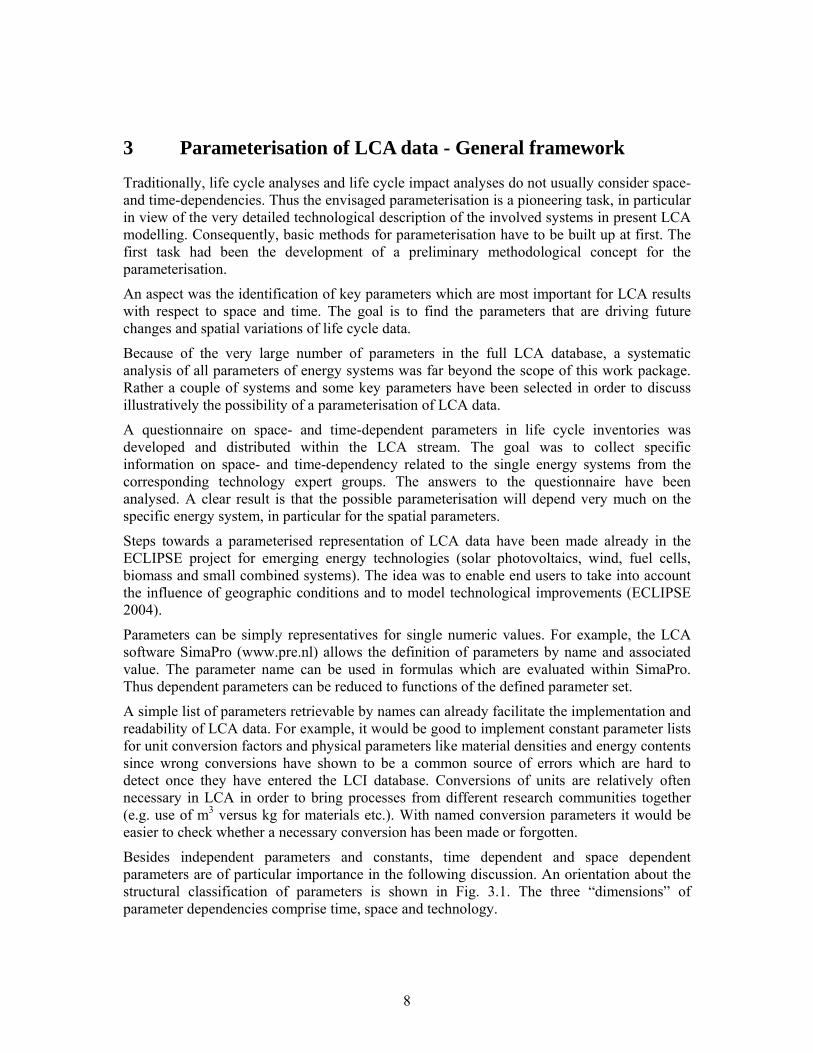
3 Parameterisation of LCA data - General framework

Traditionally, life cycle analyses and life cycle impact analyses do not usually consider space- and time-dependencies. Thus the envisaged parameterisation is a pioneering task, in particular in view of the very detailed technological description of the involved systems in present LCA modelling. Consequently, basic methods for parameterisation have to be built up at first. The first task had been the development of a preliminary methodological concept for the parameterisation.

An aspect was the identification of key parameters which are most important for LCA results with respect to space and time. The goal is to find the parameters that are driving future changes and spatial variations of life cycle data.

Because of the very large number of parameters in the full LCA database, a systematic analysis of all parameters of energy systems was far beyond the scope of this work package. Rather a couple of systems and some key parameters have been selected in order to discuss illustratively the possibility of a parameterisation of LCA data.

A questionnaire on space- and time-dependent parameters in life cycle inventories was developed and distributed within the LCA stream. The goal was to collect specific information on space- and time-dependency related to the single energy systems from the corresponding technology expert groups. The answers to the questionnaire have been analysed. A clear result is that the possible parameterisation will depend very much on the specific energy system, in particular for the spatial parameters.

Steps towards a parameterised representation of LCA data have been made already in the ECLIPSE project for emerging energy technologies (solar photovoltaics, wind, fuel cells, biomass and small combined systems). The idea was to enable end users to take into account the influence of geographic conditions and to model technological improvements (ECLIPSE 2004).

Parameters can be simply representatives for single numeric values. For example, the LCA software SimaPro (www.pre.nl) allows the definition of parameters by name and associated value. The parameter name can be used in formulas which are evaluated within SimaPro. Thus dependent parameters can be reduced to functions of the defined parameter set.

A simple list of parameters retrievable by names can already facilitate the implementation and readability of LCA data. For example, it would be good to implement constant parameter lists for unit conversion factors and physical parameters like material densities and energy contents since wrong conversions have shown to be a common source of errors which are hard to detect once they have entered the LCI database. Conversions of units are relatively often necessary in LCA in order to bring processes from different research communities together (e.g. use of m3 versus kg for materials etc.). With named conversion parameters it would be easier to check whether a necessary conversion has been made or forgotten.

Besides independent parameters and constants, time dependent and space dependent parameters are of particular importance in the following discussion. An orientation about the structural classification of parameters is shown in Fig. 3.1. The three “dimensions” of parameter dependencies comprise time, space and technology.

9

The temporal development of the single energy systems has been investigated in all technology work packages of the LCA stream within the NEEDS project. Current systems have been investigated for the reference year 2005. Scenarios have been defined for the years 2025 and 2050. Some time series show also values for intermediate years. The common scenario structure in NEEDS RS1a is a good basis for temporal parameterisation up to the year 2050. These parameters depend on time and technology.

Spatial parameterisation seems to be much more difficult than temporal parameterisation. Spatial differentiation is very diverse for the miscellaneous systems concerning importance as well as feasibility. Some specific examples will be discussed below.

The space dependency of parameters can have different reasons. For example, the space dependency may refer to local geographical conditions. A typical example for this kind of parameters is the distribution of solar irradiation as shown in Fig. 4.9 for photovoltaics and for solar thermal power. But spatial parameters can depend also on political or cultural differences e.g. in form of local legal regulations like emission limits for specific technologies.

Generally for spatial parameterisation, it can be good to couple the LCA database to a Geographical Information System (GIS). Firstly, a lot of spatial geographical information is already available in GIS formats. Secondly, modern software packages provide several functions to facilitate the processing of geographical data. For example, GIS software can calculate intersections between country data and grid data. This can facilitate the implementation of spatial data sets because the geographical resolution can be adopted to the energy system or to the availability of data.

Many LCA processes include transportation services. A GIS software is able to calculate distances for transport processes given that information about the transport path is available. For many processes, the transport distances of commodities or waste are not exactly known. Therefore NEEDS as well as other LCA projects are using standard estimates for transport distances for materials and waste. It would help to reduce inconsistencies and input errors if the assumed constant default transport distances were included as a parameter list to which all

30

35

40

45

50

2000 2010 2020 2030 2040 2050 2060

Year

Net

ele

ctric

effi

cien

cy, C

HP

200k

W (%

) Very optimisticOptimistic-realisticPessimistic t (time)

x (space)

a (technology/other)

Fig. 3.1 Orientation: Three „dimensions“ of parameterisation.

10

groups have access. If appropriate and feasible, the constant parameters could be replaced by individually calculated distances as indicated above.

The possibilities and appropriateness of spatial parameterisation differ strongly for the different energy systems. For some technologies parameterisation makes sense and simplifications are acceptable. In general one has to consider a mixture of local geographical situation, geological conditions, population structure and political decisions.

The concept of temporal and spatial parameterisation can be extended also to life cycle impact assessment. Typical examples are site-specific or country-specific impacts and external costs per ton of emitted substance for different years which can be coupled to site-specific or country-specific emission data for the technologies at corresponding time. Country-specific external cost factors have been calculated by the stream RS1b within the NEEDS project.

A proposal for a parameterised LCA database coupled to a geographical information system (GIS) is shown in Fig. 3.2. The researchers set up the collection of parameters for their technologies. A common basis of technology-independent parameters like environmental temperatures, wind speeds, solar irradiation and constants completes the technology-specific parameter collection. Space-dependent parameters are connected to a GIS. The researchers can prepare the input data with reference to the parameter set. The parameters are made transparent to the end users. In some cases it makes sense that also the end user can select or modify parameters for his or her calculations for example to check the influence of assumptions on the final results.

Fig. 3.2 Possible structure of a parameterised LCI and LCIA database. (m = number of processes, n = number of flows to and from nature, r = number of LCIA methods, p = parameter, a = technology, t = time, x = space).

Parameters:

input process matrix

(m x m)

cumulative process matrix

(m x m) cumulative LCI

results (n x m)elementary

flow matrix (n x m)

LCIA methods matrix (r x n)

rese

arch

ers /

dat

a su

pplie

rs

end

user

s

cumulative LCIA results (r x m)

indep. p p(a,t) p(a,t,x) GIS

11

4 Examples of time-, technology-, and space-dependent parameters

In this chapter we discuss a couple of explicit examples of parameters from different energy systems under the perspective of time-dependency, technology-dependency, and space-dependency. This should illustrate in an exemplary way the potential of an advanced parameterised LCA model.

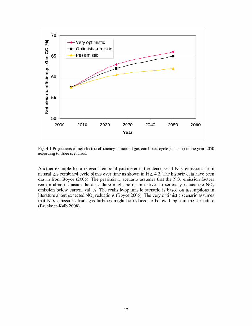
4.1 Time-dependency In the NEEDS project, the future development of energy technologies and LCA background processes up to the year 2050 have been estimated. Three types of scenarios have been developed, pessimistic, realistic-optimistic and very optimistic ones. For example, Fig. 4.1 shows the estimated projections of the net electric efficiency of natural gas combined cycle power plant in the 400-500 MWe class between 2005 and 2050 for three scenarios. It is widely believed in literature that the gas combined cycle plant will reach an efficiency of about 65% but not much more in future (e.g. DWTC 2001, Bachmann 2004). This value has been assigned to the year 2050 in the realistic-optimistic scenario for full load operation. Alternative designs like fuel cell/gas turbine hybrid plants (not discussed here) promise efficiencies of 70% or beyond in future. The electric efficiency of the plant has direct influence on the LCA results because the higher the efficiency the lower are the environmental burdens and external costs per kWhe. For scenario implementation it has to be considered that the efficiency depends also on the load (Boyce 2006). For the projected efficiencies shown here it was assumed that the plant is operating predominantly in full load mode.

In a similar way as shown by the example (Fig. 4.1), temporal key parameters for different energy technologies have been established in NEEDS (see the technology reports of the different work packages in NEEDS stream RS1a). In most cases, the base years 2005, 2025 and 2050 are used. The common format is a good basis for the parameterisation of temporal parameters based on scenario assumptions.

12

50

55

60

65

70

2000 2010 2020 2030 2040 2050 2060

Year

Net

ele

ctric

effi

cien

cy ,

Gas

CC

(%) Very optimistic

Optimistic-realisticPessimistic

Fig. 4.1 Projections of net electric efficiency of natural gas combined cycle plants up to the year 2050 according to three scenarios.

Another example for a relevant temporal parameter is the decrease of NOx emissions from natural gas combined cycle plants over time as shown in Fig. 4.2. The historic data have been drawn from Boyce (2006). The pessimistic scenario assumes that the NOx emission factors remain almost constant because there might be no incentives to seriously reduce the NOx emission below current values. The realistic-optimistic scenario is based on assumptions in literature about expected NOx reductions (Boyce 2006). The very optimistic scenario assumes that NOx emissions from gas turbines might be reduced to below 1 ppm in the far future (Brückner-Kalb 2008).

13

1

10

100

1000

1970

1980

1990

2000

2010

2020

2030

2040

2050

NO

x em

issi

ons

GT+

CC

(mg/

MJi

n) historic datapessimisticrealistic optimisticvery optimistic

Fig. 4.2 Historic and projected development of NOx emissions from natural gas combined cycle plants over time.

The implementation of time series for time-dependent parameters is straightforward. Nevertheless, it is an interesting question whether further simplifications may be possible and advantageous.

A well-known approach to modelling the future costs of technologies is the method of experience curves. Experience curves give the relation between specific investment costs C and cumulative production P (in terms of installed power or number of units produced):

b

PP

CC

−

⎟⎟⎠

⎞⎜⎜⎝

⎛=

0

1

0

1 .

Here C0 and P0 are the costs and cumulative production at a certain reference time. The costs C1 at a later time can be estimated from the cumulative production P1 at this time. b is the learning index or learning elasticity.

A corresponding experience curve approach for emissions or other environmental burdens E of technical devices would be

14

b

PP

EE

−

⎟⎟⎠

⎞⎜⎜⎝

⎛=

0

1

0

1 ,

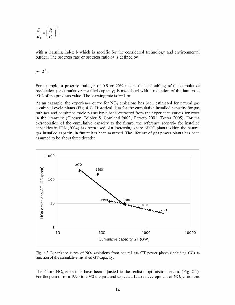
with a learning index b which is specific for the considered technology and environmental burden. The progress rate or progress ratio pr is defined by

pr=2-b.

For example, a progress ratio pr of 0.9 or 90% means that a doubling of the cumulative production (or cumulative installed capacity) is associated with a reduction of the burden to 90% of the previous value. The learning rate is lr=1-pr.

As an example, the experience curve for NOx emissions has been estimated for natural gas combined cycle plants (Fig. 4.3). Historical data for the cumulative installed capacity for gas turbines and combined cycle plants have been extracted from the experience curves for costs in the literature (Claeson Colpier & Cornland 2002, Barreto 2001, Tester 2005). For the extrapolation of the cumulative capacity to the future, the reference scenario for installed capacities in IEA (2004) has been used. An increasing share of CC plants within the natural gas installed capacity in future has been assumed. The lifetime of gas power plants has been assumed to be about three decades.

1

10

100

1000

10 100 1000 10000

Cumulative capacity GT (GW)

NO

x em

issi

ons

GT+

CC

(ppm

)

20302010

2000

19801970

1990

Fig. 4.3 Experience curve of NOx emissions from natural gas GT power plants (including CC) as function of the cumulative installed GT capacity.

The future NOx emissions have been adjusted to the realistic-optimistic scenario (Fig. 2.1). For the period from 1990 to 2030 the past and expected future development of NOx emissions

15

from GT and CC can be approximately represented by an experience curve with a progress ratio of about 78%.

The possible advantage of such a parameterisation compared to few fixed scenarios is a higher flexibility in modelling of the future development of emissions. Different assumptions about the future installed capacities would imply different emission scenarios based on the assumption of continuous improvements of the devices. The assumptions can be adjusted (e.g. to very optimistic or pessimistic scenarios) by assuming appropriate learning indices.

Nevertheless, the extension of the experience curves to emissions and other environmental burdens should be seen with some scepticism as the historic part of the GT NOx example shows (Fig. 4.3). Formally, the GT NOx emissions have decreased between the years 1970 and 2000 with a progress ratio of approximately 40%. But between 1980 and 1990 the NOx emissions jumped down dramatically, probably because of political pressure due to legal regulations (like e.g. the large combustion plant directive of the European Union which has been proposed in 1983 and adopted in 1988). This shows that the development is not necessarily as steady-going as the experience curve approach would suggest.

Fig. 4.4 shows the past development and projected future development of the electric efficiency of natural gas combined cycle plants. Because the gas turbine is the key component of the CC, the cumulative capacity of GT has been chosen as independent variable. The electric efficiencies have been approximately adjusted to the realistic-optimistic scenario until 2030 and to the IEA reference scenario for natural gas (IEA 2004). The experience curve derived for the time between 1990 and 2030 has a progress ratio for the losses (=100% minus electric efficiency) of about 95%. It has to be considered that the electric efficiency curve is assumed to flatten around about 65% in the further development.

10%

100%

10 100 1000 10000

Cumulative capacity GT (GW)

CC

ele

ctric

effi

cien

cy (%

)

1990 2000 2010 20302020

1980

Fig. 4.4 Development of the electric efficiency of natural gas combined cycle plants as function of the cumulative GT capacity.

16

The generalisation of the experience curve approach to environmental burdens opens an interesting possibility for the modelling of future scenarios. Nevertheless, the approach has to be handled with care. The time development of emission factors seems generally not as simple as in the case of cost experience curves. The reason is probably that there is no constant pressure to improve the environmental performance continuously unlike in the case of internal costs where the market pressure permanently favours cost reductions. Nevertheless, in some cases the use of environmental experience curves could be applicable. This would need further investigation.

4.2 Technology-dependency A possible benefit of parameterisation for reducing the complexity of LCA is the avoidance of unnecessary redundancy. For example, it is often very difficult or even impossible to get real measured emission data separately for each country and for every substance in the database. Therefore, emission factors are often transferred to other locations. In the current version of the ecoinvent database, assumptions about emission factors for different countries with identical or similar technology are simply repeated. The implementation is well documented in reports, but not necessarily very transparent on the level of the database. The introduction of commonly used parameters can be helpful to improve the readability.

Examples are emissions of NMVOC (Non-Methane Volatile Organic Compounds). NMVOC comprises a set of organic substances which can be toxic or which play a role as precursors of ozone or organic particulate formation. In ecoinvent, NMVOC emissions can be entered as a whole or as separate species. A list of the NMVOC components is provided in the ecoinvent documentation. It would be helpful if such a list were implemented directly in the database so that the total NMVOC can be calculated immediately.

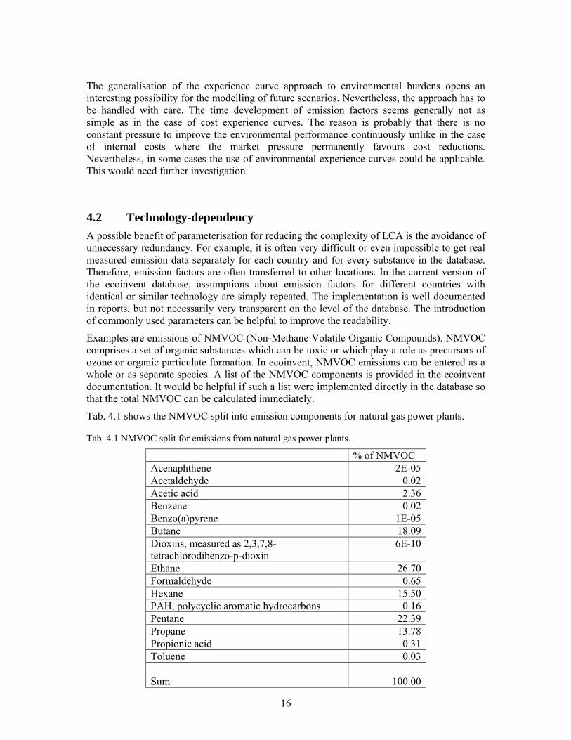
Tab. 4.1 shows the NMVOC split into emission components for natural gas power plants.

Tab. 4.1 NMVOC split for emissions from natural gas power plants.

% of NMVOC Acenaphthene 2E-05 Acetaldehyde 0.02 Acetic acid 2.36 Benzene 0.02 Benzo(a)pyrene 1E-05 Butane 18.09 Dioxins, measured as 2,3,7,8-tetrachlorodibenzo-p-dioxin

6E-10

Ethane 26.70 Formaldehyde 0.65 Hexane 15.50 PAH, polycyclic aromatic hydrocarbons 0.16 Pentane 22.39 Propane 13.78 Propionic acid 0.31 Toluene 0.03 Sum 100.00

17

The NMVOC split vector can be assumed approximately constant for all countries. The inclusion of NMVOC splits or similar splits (like the further split of PAH into components if available) as technology-specific parameters would reduce the number of parameters as shown in Fig. 4.5. The avoidance of such redundancies improves the transparency of the database.

NMVOCsplit

NMVOCemissionsNMVOC

emissionsNMVOCemissionsNMVOC

emissionsNMVOCemissionsNMVOC

emissionsNMVOCemissionsNMVOC

emissionsNMVOCemissions

k species

N locations * k species

model

calculated

Fig. 4.5 Schematic reduction of redundancy by use of a parameter set for the technology specific NMVOC split. For N countries and k species, the number of parameters is reduced from N*k to k.

The parameters used in LCA modelling commonly depend on the technology considered. If the technology dependency can be expressed by an explicit functional dependency, the correlations can be used to further reduce the number of independent parameters and to systematise the modelling.

For example, Fig. 4.6 shows the dependency of the specific weight in terms of kg/kW of small natural gas combined heat and power plants on the input power. The material needed for the CHP plant per kW decreases with increasing input capacity. In the range between about 20 and 5000 kW, the specific weight follows approximately a power law with an exponent of about -1/3. (This specific power law is restricted to small CHP plant because the specific weight cannot tend to zero for very large plants.) The smaller the CHP plant, the more important are the infrastructure material requirements for the plant in relative terms.

18

y = 80.172x-0.3314

R2 = 0.9221

0

5

10

15

20

25

0 1000 2000 3000 4000 5000x = Input Power (Natural Gas) [kW]

y =

Spec

ific

Wei

ght [

kg/k

W]

Fig. 4.6 Specific weight of small natural gas CHP plants depending on the input power (Source: Heck 2004).

In a similar way, the electric and thermal efficiencies of CHP plants depend on the size of the plant. Fig. 4.7 shows the electric, thermal, and total efficiencies of small natural gas CHP plants as functions of the fuel input power of the plant. Fig. 4.8 shows the same parameters for small biogas CHP plants as functions of the electric output.

19

0%

10%

20%

30%

40%

50%

60%

70%

80%

90%

100%

0 1000 2000 3000 4000 5000Input Power (Natural Gas) [kW]

Effic

ienc

y [%

]

TotalThemalElectric

Fig. 4.7 Electric, thermal, and total efficiencies of small natural gas CHP plants as functions of the capacity (Source: Heck 2004).

Fig. 4.8 Electric, thermal, and total efficiencies of small biogas CHP plants as functions of the capacity (Source: Tehlar 2007).

20

The electric efficiency of small CHP plants increases with increasing size of the plant, whereas the thermal efficiency decreases with size. The total CHP efficiency changes only slightly with size.

The dependency of the efficiency together with the dependency of the material use on the size of CHP plants can be used to implement a range of CHP capacities (roughly between 20 and 5000 kW) in a parameterised form into the LCI database. Currently, several sizes of CHP plants are included in the ecoinvent database separately. With a consequent parameterisation, users could choose freely a plant size and get the results based on the parameter calculations.

The operating CHP plant produces electricity and heat. It is an example for what is called a “multi-output process”. For multi-output processes, the question is how environmental burdens should be allocated to the single outputs. Allocation is necessary for example if a specific output from a multi-output process should be used in other processes or if it should be compared to the output of a single-output process e.g. electricity from CHP plants compared to electricity from pure electricity plants. The allocation scheme can have strong influence on the results. The current EcoSpold format allows the definition of allocation factors; insofar a parameterisation is already considered on the level of data exchange. Nevertheless, it would be good if the allocation assumptions were more transparent to the end user. The allocation factors should be adjustable or selectable by the end user but based on well-founded default values.

Another important set of LCA parameters are the recycling rates for waste and the shares of recycling within the material production. In the current ecoinvent database and in the NEEDS database, the recycling shares are not very transparent although these factors can be found in the documentation. The contributions of recycling processes have strong effect on the environmental burdens of materials and material-intensive systems. In particular for future scenarios, the assumptions on recycling may significantly influence the LCA results. Therefore, at least the recycling shares should be brought more into the foreground. This is independent from the question how detailed the recycling processes themselves should be treated.

4.3 Space-dependency An example for a space-dependent parameter due to natural variation is the annual solar irradiation as shown in Fig. 4.9. For photovoltaics and solar thermal plants, the annual electricity generation (yield in kWhe/a per installed kWp) depends on the local annual solar irradiation (kWh/(m2*a)).

21

Fig. 4.9 Photovoltaic potential in Europe. Yearly sum of global irradiation on an optimally-inclined surface based on 10-years average of the period 1981-1990 [kWh/(m2*year)] (Source: Šúri et al. 2007, http://re.jrc.ec.europa.eu/pvgis/).

If the LCA model is connected to a database of solar irradiation data (ideally in a GIS database), site-specific LCA results can be calculated and provided to the end user.

Another class of space-dependent parameters that could be systematically treated to a certain extent in an advanced LCA model are infrastructure parameters related to the locations of energy installations. The cables for the transmission of electricity from power plants which are located far away from populated or industrialized areas to the electricity grid can contribute substantially to the LCA burdens of the plant. This applies for example to remote wind farms, to off-shore wind plants or to remote solar power plants.

The material needs for the transmission line of length L can be calculated from the location of the plant relative to the grid as outlined in Fig. 4.10.

22

Fig. 4.10 Transmission line of length L from power plant to electricity grid.

The relationships for the material needs can be found in the literature on electro-technology. The required cross-sectional area q of the cable (e.g. of copper) can be estimated by the formula (Böge 1999)

LUp

Pql )(cos22 ϕ

ρ=

with

P power of the plant

ρ specific electrical resistance of the metal

pl tolerable power loss

U voltage

cos(φ) phase factor for alternating current (typically cos(φ)≈0.85)

L length of transmission cable.

With the mass density µ of the metal, the total metal mass requirement M of the cable for the LCA input can be estimated by

222 )(cos

LUp

PMl ϕ

µρ= .

Lgrid

power plant

23

For practical purposes, it is often convenient to use a reference system which has been already analysed for the assessment of further plants. Assumed that the material of the cable and the tolerable power loss remain the same as for the reference plant, the total metal mass M of the newly assessed plant can be estimated by

2

2

2

2

ref

ref

refref L

LUU

PPMM ⋅⋅=

where Mref, Lref and Uref are mass of metal, length and voltage of the reference transmission line and Pref is the power of the reference plant.

The length L can be automatically calculated in a GIS software when the location of the plant and the GIS data for the grid are given, so that, once the GIS model with basic data is established, only the position and the power of the plant and the voltage of the transmission line have to be defined. In principle, the mass requirements for the transmission lines should be considered for all power plants (at least the large ones), so that a GIS model of the transmission lines would be advantageous for the LCA of all grid-connected electricity systems.

Similar models for an advanced GIS-coupled LCA system could be developed for the pipelines or transport routes of other energy carriers like oil, natural gas, gas from biomass, or hydrogen.

Emission data for the power plant entered into the GIS database for the specified location can be used to perform site-specific environmental and external cost assessment in connection with LCA.

There are also space-dependent parameters for completely different reasons. Examples are differences due to country-specific or local legal regulations of emissions.

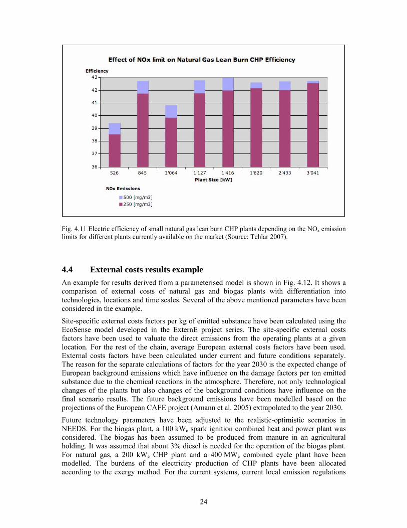
Fig. 4.11 shows the influence of NOx emission limits defined by legal regulations on the electric efficiency of natural gas lean burn CHP plants which are currently available on the European market. The reduction of NOx emissions implies a reduction of the electric efficiency. Thus the emission regulations do not only influence the emission factors of the power plant but also the burdens due to the influence on efficiency.

24

Fig. 4.11 Electric efficiency of small natural gas lean burn CHP plants depending on the NOx emission limits for different plants currently available on the market (Source: Tehlar 2007).

4.4 External costs results example An example for results derived from a parameterised model is shown in Fig. 4.12. It shows a comparison of external costs of natural gas and biogas plants with differentiation into technologies, locations and time scales. Several of the above mentioned parameters have been considered in the example.

Site-specific external costs factors per kg of emitted substance have been calculated using the EcoSense model developed in the ExternE project series. The site-specific external costs factors have been used to valuate the direct emissions from the operating plants at a given location. For the rest of the chain, average European external costs factors have been used. External costs factors have been calculated under current and future conditions separately. The reason for the separate calculations of factors for the year 2030 is the expected change of European background emissions which have influence on the damage factors per ton emitted substance due to the chemical reactions in the atmosphere. Therefore, not only technological changes of the plants but also changes of the background conditions have influence on the final scenario results. The future background emissions have been modelled based on the projections of the European CAFE project (Amann et al. 2005) extrapolated to the year 2030.

Future technology parameters have been adjusted to the realistic-optimistic scenarios in NEEDS. For the biogas plant, a 100 kWe spark ignition combined heat and power plant was considered. The biogas has been assumed to be produced from manure in an agricultural holding. It was assumed that about 3% diesel is needed for the operation of the biogas plant. For natural gas, a 200 kWe CHP plant and a 400 MWe combined cycle plant have been modelled. The burdens of the electricity production of CHP plants have been allocated according to the exergy method. For the current systems, current local emission regulations

25

have been considered. Tab. 4.2 shows the assumed NOx emission factors for small CHP plants which differ due to local emission regulations.

Tab. 4.2 Assumed NOx emissions from small natural gas and biogas CHP plants according to legal emission limits (Source: Tehlar 2007).

Location Natural gas CHP Biogas CHP

mg/Nm3 (5% O2) mg/Nm3 (5% O2)

Germany 500 500

Switzerland, generally 250 400

Basel, Switzerland 70 200

Zürich, Switzerland 50 50

The external costs results per kWhe for different systems are shown in Fig. 4.12. (For Greenhouse Gases (GHG), external costs of 19 Euro/ton CO2-equivalent have been assumed according to European Commission (2005).)

00.20.40.60.8

11.21.41.61.8

biog

as D

E (R

osto

ck)

biog

as C

H (N

orth

)

biog

as Z

üric

h

biog

as B

asel

NG

CH

P D

E (R

osto

ck)

NG

CH

P C

H (N

orth

)

NG

CH

P Z

üric

h

NG

CH

P B

asel

NG

CC

CH

biog

as C

H (N

orth

)

NG

CH

P C

H (N

orth

)

NG

CC

CH

Current systems 2030

Exte

rnal

cos

ts (E

UR

-cen

t20

00/k

Whe

)

Ionising RadiationSulfates, primaryNitrates, primaryNMVOC (via O3)FormaldehydeNickelLeadChromium-VICadmiumArsenicPM2.5-10PM2.5NOxSO2GHG (IPCC 100a)

Fig. 4.12 Comparison of external costs related to natural gas and biogas plants. The figure shows different technologies, different locations and different times.

The comparison shows the influence of the different parameters. The external costs of natural gas systems, in particular those of the combined cycle plants, are dominated by the CO2

26

emissions. By contrast, the external costs of the biogas CHP plants are dominated by the secondary particulates (nitrates) formed in the atmosphere from NOx emissions.

A biogas plant operating currently with the maximum allowed NOx emissions (400 mg/Nm3) in Switzerland (CH) causes approximately the same external costs per kWe as a natural gas combined cycle plant (NG CC), where in the first case the major contribution stems from NOx and in the second case from Greenhouse Gas (mainly CO2) emissions (compare second and ninth column in Fig. 4.12).

For current biogas plants, also SO2 emissions are significant. It was assumed that the biogas is purified by biological desulphurisation.

The biogas plant located in Rostock (Germany) has lower external costs than the same plant located in Northern Switzerland although the NOx emission limits in Germany are higher than in Switzerland. The reason is that Rostock is located at the coast. As a rule of thumb, assumed that the wind vector distribution is not too asymmetric, the NOx, SO2, and PM emitted at a coast cause roughly half of the damages compared to an inland location with the same population density because the external costs are dominated by human health effects (including mortality) which vanish approximately for the half of emissions which are blown to the open ocean. Among the biogas plants, the plants in Zürich have the lowest external costs because of the strict emission limits.

The example shows that different competing parameters have strong influence on the results. An appropriate parameterisation must take into account site-specific effects, technological specialities, political boundary conditions and temporal developments simultaneously.

27

5 Selected parameters of electricity generation systems

This chapter gives an overview on important spatial and temporal parameters for single energy systems. The focus is mainly on energy systems which have been investigated in the NEEDS project. The structure of the spatial and temporal parameter sets depends strongly on the specific energy system.

5.1 Advanced fossil In section 5.1.1, important spatial parameters related to advanced fossil power systems (coal and natural gas) and carbon capture and sequestration are collected. Section 5.1.2 discusses temporal parameters for fossil systems.

5.1.1 Spatial parameters

5.1.1.1 List of parameters The following lists show a qualitative overview of relevant spatial parameters for the different fossil systems.

All advanced fossil power plants

The following space-dependent parameters refer to all fossil systems: • Efficiency of power plant as function of ambient temperature. • Emissions as functions of legal regulations. Emissions depend on emission limits

defined by local emission regulations. This concerns all plants (power plants but also industrial plants) in the chain. (The regulations can vary even within countries. E.g. the Swiss air protection law (“Luftreinhalteverordnung”, LRV) defines emission limits for Switzerland but some Swiss Cantons apply stricter rules for special areas).

• Efficiency as function of legal regulations. The efficiency of power plants can depend on local emission regulations. Efficiency of gas motor CHP and gas turbine/GCC/IGCC can depend on local NOx emission limits (which have influence on the maximum temperature of the process). Efficiency can be reduced also by filters (e.g. scrubbers for SO2 reduction). CO2 capture reduces efficiency; there could be local regulations in future although the effects of the emissions are global; additional processes related to CO2 capture in order to separate undesirable substances may have implications on total efficiencies as well.

Natural gas Particularly for natural gas, the following major spatial parameters are important (besides the general parameters for all fossil systems mentioned above):

• Upstream burdens of natural gas supply. LCA chain of natural gas depends on country-specific gas supply. Particular space-dependent parameters:

• origin of natural gas, • length of gas pipelines (gas transport distances), • leakage rates of gas pipelines, • efficiencies of compressor stations (age-dependent), • emissions factors of gas turbines of compressor stations (age-dependent), • share of liquefied natural gas.

28

The gas supply chain has influence on the cumulative emissions (e.g. total GHG emissions) but also on the spatial distribution of classical pollutants (e.g. NOx, SO2, PM) which cause local and regional damages.

• Natural gas composition. The gas composition (which influences emission factors and heating value) depends on the origin of the natural gas and on the purification process. Nevertheless, the variation of the gas composition in Europe is rather small i.e. the effect can be neglected in a first approximation.

Hard coal • Hard coal characteristics:

• Elementary composition: depends on origin of coal. Emission factors of power plants may depend on factors like sulphur content, humidity, trace element and ash content of the coal delivered to the power plants.

• Heating value: may change with origin of coal. Emission factors per kWh produced electricity and cumulative upstream burdens both depend on the heating value.

• Origin of hard coal supply mix: shares of production regions to hard coal supply mixes are country-specific. Since cumulative LCA results per kg hard coal depend on the production region (specific CH4 emissions, heating value, transport mode and distance, etc.), these shares determine the cumulative upstream burdens of the hard coal chain as well as the spatial distribution of impacts (e.g. due to NOx, SO2, PM).

Lignite • Lignite characteristics:

• Elementary composition: may change with origin of lignite. However, current modelling of the lignite chain includes only average European lignite with uniform composition.

• Heating value: may change with origin of coal. Emission factors per kWh produced electricity and cumulative upstream burdens both depend on the heating value. However, current modelling of the lignite chain includes only average European lignite with uniform composition.

Carbon Capture and Storage

• Transport lines and distances for carbon transport.

• Depth of carbon repository.

• Usability of old natural gas pipelines for CO2 transport to depleted gas fields.

5.1.1.2 Geographical reference data related to system parameters

The table Tab. 5.1 below gives an overview on proposed geographical reference data that might be used to characterize the space-dependency of important system parameters of fossil systems. Generally, the appropriate geographical resolution depends on the goals of the analysis. The following table provides some suggestions for the geographical reference data that might be used by a standard parameterized model.

29

Tab. 5.1 Proposed geographical reference data for selected spatial parameters of fossil systems.

System Geographical reference data / resolution

Data available at For parameter(s)

Annual average ambient temperature

Global Historical Climatology Network (cdiac.ornl.gov)

Efficiency of power plant

Local cooling conditions (water/air)

Local information Efficiency of power plant

Country (or administrative units) Emissions as functions of legal regulations

All adv. fossil

Country (or administrative units) Efficiency as function of legal regulations

Country ecoinvent Upstream burdens of natural gas supply

GIS polygons Routes of pipelines

Natural gas

Country ecoinvent Natural gas composition Country Literature Characteristics of hard

coal supply mix (country-specific)

Hard coal

Country ecoinvent, new statistics, projections & scenarios

Origin of hard coal (country-specific)

Lignite Country ecoinvent Heating value GIS polygons Carbon transport lines CCS

Geological information Depth of carbon repository

5.1.1.3 Steps towards quantification

Efficiency of power plant as function of ambient temperature: The location of the thermal power plant has influence on the efficiency achievable for a given technology and a given mode of operation. The minimal temperature related to the Carnot efficiency of thermal electricity production depends on the cooling conditions (e.g. the temperature of the river from which the cooling water is extracted). The lower the ambient temperature the higher is the possible efficiency of the plant. Thus, the possible annual average efficiency depends on the annual average ambient temperature of the region but also on the detailed local conditions e.g. the distance between plant and cooling water source. Condenser pressure as function of ambient temperature influences thermal efficiency.

• Quantification, in principle, simplified: The Carnot efficiency η depends on the environmental temperature TE which in turn depends on the location x:

effU

E

TxT

,

)(1−=η

30

(the effective upper temperature of the process TU,eff is determined by the technology). In a simple idealised model with an upper temperature of about 1300°C for a gas combined cycle plant with electric efficiency at about 58 %, assumed that the lower temperature of the process is close to the environmental temperature and that the ratio between efficiency and Carnot efficiency is constant, an increase of the environmental temperature of 10°C implies a decrease of the efficiency of roughly 0.5 percent points.

• In a simple implementation, a table with annual average temperatures for countries may be used to estimate spatial variations of the achievable efficiencies relative to a reference location. Additionally, an interactive user interface might be used to ask for more detailed local temperature conditions if available for the assessment of a specific system.

Legal regulations concerning emission limits of small combustion plants like natural gas and diesel combined heat and power plants have to be considered. The local variations of such regulations for small plants in Europe and even within some countries make it difficult to keep a database up to date.

Emission regulations influence not only the direct emissions from the operating plant but also have impact on the performance of the plant. Fig. 4.11 shows the influence of NOx emission limits defined by legal regulations on the electric efficiency of natural gas lean burn CHP plants which are currently available on the European market. The reduction of NOx emissions implies a reduction of electric efficiency and thus an increase of fuel input per kWh electricity. Both, the direct emissions from the plant but also the efficiency, are important parameters for the life cycle assessment of the system.

5.1.1.4 Conclusions on the space-dependency of life cycle results

Natural gas power plants

• The direct CO2 emissions from operating natural gas combined cycle power plants can be derived from the space-dependent efficiency as a function of the annual ambient temperature, assumed that the variation of the gas composition is negligible or that the local gas composition is known.

• Similarly other direct emissions from the operating plant which depend only on the gas composition (SO2, heavy metals) provided that the local gas composition is known or can be assumed constant.

• Warning: No direct conclusions should be drawn about the full chain greenhouse gas emissions per kWhe for natural gas plants because they depend also on the country-specific gas supply chain. However, once the upstream characteristics are known (or fixed e.g. by modelling scenarios) the parameters become functions of the efficiency.

Hard coal power plants

• The direct CO2 emissions from the operation of a specific hard coal power plant technology can be derived from the space-dependent efficiency as a function of the annual ambient temperature, assuming constant (average) CO2 emissions per MJ hard coal.

• Warning: No direct conclusions should be drawn about greenhouse gas emissions of the complete hard coal chain per kWhel, because they also depend on the country-

31

specific hard coal supply mixes (upstream) and to a much smaller extent on construction and dismantling of the power plant infrastructure.

Lignite power plants

• Given the fact that contributions of construction and dismantling of the power plant infrastructure to cumulative LCA results are very minor, mainly power plant efficiency and to a smaller extent heating value of lignite dominate cumulative LCA results. Therefore, if one of these parameters is kept constant, preliminary quantitative conclusions about space-dependency of the cumulative LCA results can be drawn.

5.1.2 Time-dependent parameters The following section gives an overview on key parameters of fossil systems that may change over time.

5.1.2.1 List of parameters

Gas turbine + Gas CC

• Efficiency of gas turbine and CC as function of maximum temperature (firing temperature) of gas turbine cycle, depending on the development of materials for the hot-section components of the gas turbine.

• Efficiency of gas turbine and CC as function of pressure ratio of gas turbines.

• Lifetime of power plant.

• Mode of operation (full load hours per year). Because of the flexibility of natural gas power plants, the mode of operation is particularly important for this system. It depends on the development of the whole energy system e.g. on the future needs of base-load power or backup for renewable energy systems.

• Specific land use per kWhe (if a power plant with the same size has a higher efficiency, the land use per kWhe decreases).

• Leakage rate of gas pipelines, depending on installation of new pipelines.

• Upstream burdens of natural gas supply depend on the country-specific supply structure which may change over time (share of own production, share of imports and origin of gas). The supply structure depends also on the economic and political situation (e.g. natural gas imports from Russia).

• Gas composition. The gas composition depends on the origin of the natural gas and on the purification process. The natural gas supply structure of a country may change over time for economic and political reasons. Nevertheless, the variation of the gas composition in Europe is rather small i.e. the effect can be neglected in a first approximation.

Hard coal PC

• Efficiency of hard coal power plants as function of maximum temperature (firing temperature) of boiler, depending on stress resistance of materials.

32

• Lifetime of power plant.

• Mode of operation (full load hours per year).

• Country-specific origin of hard coal supply mixes which in turn depends on the economic and political situation.

• Hard coal characteristics, which depends on the origin of hard coal. The hard coal supply structure of a country may change over time for economic and political reasons.

Hard Coal IGCC

• Technical life time of the power plant

• Efficiency:

• Efficiency increase by hot gas clean up: pollutant removal (dust removal, desulphurisation) from higher temperature gas streams.

• The anticipated increase of efficiency is directly coupled with the development of gas turbine technology. An important step is the development of improved syngas turbines with materials applicable by 650°C and later on by 700°C.

• Membrane technology may also become important for separating gases produced by coal gasifiers or for the provision of oxygen for the gasification process. Considerable energy saving and cost reduction is expected from membranes for O2 separation.

• Availability: Development of materials to ensure greater reliability, especially refractories, improved dry feeding, improved fire-tube cooler designs with regard to minimising deposition and corrosion.

Lignite

• Efficiency of lignite power plants as function of maximum temperature (firing temperature) of boiler, depending on stress resistance of materials.

• Lifetime of power plant.

• Mode of operation (full load hours per year); this might be essentially base load for lignite.

• Lignite characteristics, especially the heating value, which depends on the origin of lignite and therefore on the location of the power plant (operated mine-mouth).

Carbon Capture and Storage

• Energy demand for CO2 capture and compression (“efficiency penalty”).

33

5.1.2.2 Steps toward quantification

For the future efficiency of gas turbine plants, gas combined cycle plants and IGCC plants, the development of gas turbine technology is important. Between the 1970s and the early 2000s, gas turbine inlet temperatures increased from about 800 to 1230°C (Pauls 2003). During this time, the efficiency of gas turbines raised from 28% to over 38%. The Siemens V94.3A gas turbine achieves an efficiency of 38.6% (Pauls 2003). In the 1970s, gas turbine capacities were limited to about 50 MWe. A modern gas turbine like the Siemens V94.3A exceeds a capacity of 260 MWe. Standalone gas turbines are relatively inefficient power sources compared to combined cycle plants. The advantages of gas turbines are low capital costs, low maintenance costs, and fast completion time to full operation (Boyce 2002).

GT efficiency as functions of firing temperature and pressure ratio: In order to achieve the optimum thermal efficiency of a gas turbine, it is necessary to increase both, the firing temperature and the pressure ratio. Gas turbines for electricity production are optimized with the objective of a long lifetime. This sets limits to the firing temperature and pressure ratio. By contrast, the gas turbines for aircrafts are designed for a much shorter lifetime and therefore are operating at higher temperatures and higher pressure ratios reaching higher efficiencies compared to stationary gas turbines. The development of the firing temperature of stationary gas turbines over time had a complex shape as a function over time during the past decades. The firing temperature increased from about 750°C in the 1950s to about 950°C in the late 1970s (Boyce 2002). It tended to level off in the early 1980s. The introduction of the “aero-derivative gas turbine” led to a dramatic improvement of firing temperatures of industrial gas turbines in the 1990s from about 1000°C to about 1350°C around year 2000 (Boyce 2002). The pressure ratio of gas turbines as a function over time follows a similar shape. The pressure ratio has increased from about 17 in 1980 to about 35 around year 2000 (Boyce 2002).

Breakthroughs in blade metallurgy and new concepts of air-cooling have been important prerequisites to achieve high inlet temperatures for gas turbines (Boyce 2002).

The efficiency of the gas turbines increases with increasing firing temperature. The dependency of the efficiency on the pressure ratio at a given temperature is not a simple monotone function. At first, the increase of the pressure ratio leads to an increase of the efficiency. But increasing the pressure ratio beyond a certain value can lower the overall cycle efficiency at a given firing temperature. The optimum pressure ratio for a simple cycle at turbine inlet temperature of 1650°C is about 40:1. In a regenerative cycle (i.e. if a regenerator is used in order to increase the efficiency of the gas turbine), the optimum pressure ratio at 1650°C is about 20:1. Furthermore, very high pressure ratios result in a reduced tolerance of the turbine compressor to dirt in the inlet air filter and on the compressor blades (Boyce 2002).

A study by General Electric for the US Department of Energy (DOE) investigated key design parameters of next generation gas turbines (NGGT). A hybrid aero-derivative/heavy duty concept was identified as being the top candidate technology with a time horizon 2010 for development and availability for demonstration testing. The firing temperatures and the net plant efficiencies of future gas turbine designs were classified confidential whereas the pressure ratio has been disclosed (General Electric 2001, table 2.1.4).

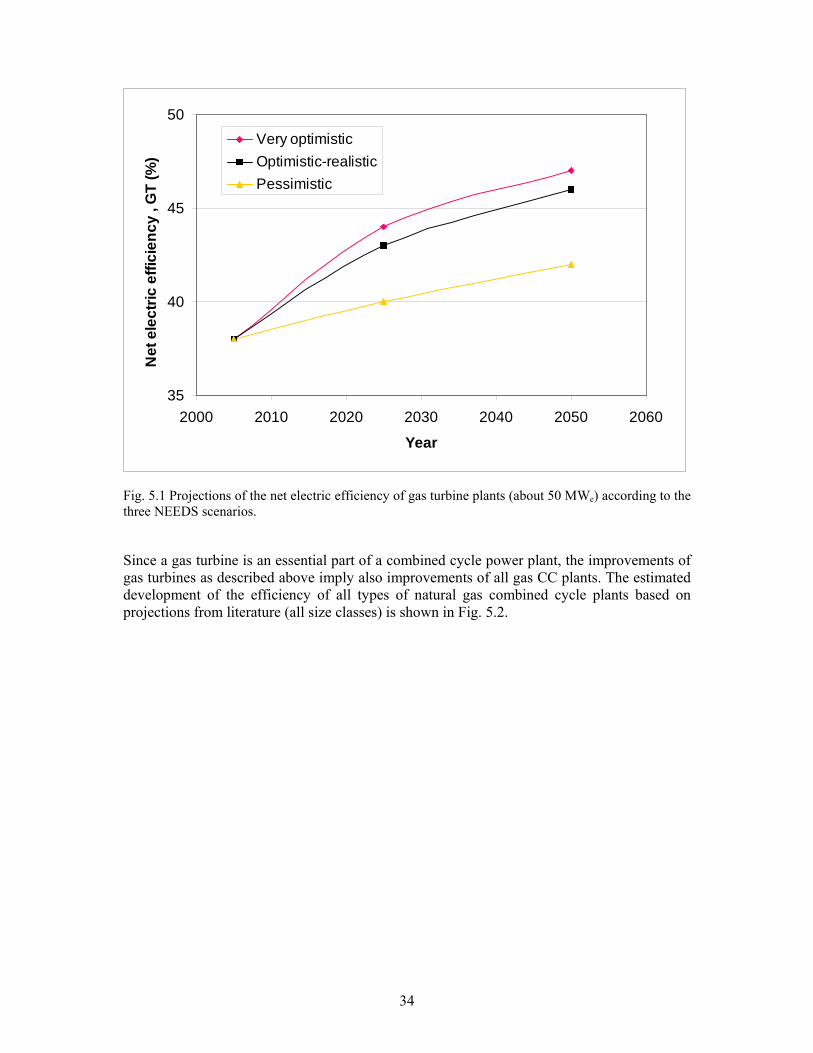
Fig. 5.1 shows the estimated development of the electric efficiencies of natural gas turbine plants until year 2050 for the three scenarios of the NEEDS project. The development of efficiencies of natural gas combined cycle plants assumed according to the three NEEDS scenarios in the 400-500 MWe class for full load operation are shown in Fig. 4.1.

34

35

40

45

50

2000 2010 2020 2030 2040 2050 2060

Year

Net

ele

ctric

effi

cien

cy ,

GT

(%)

Very optimisticOptimistic-realisticPessimistic

Fig. 5.1 Projections of the net electric efficiency of gas turbine plants (about 50 MWe) according to the three NEEDS scenarios.

Since a gas turbine is an essential part of a combined cycle power plant, the improvements of gas turbines as described above imply also improvements of all gas CC plants. The estimated development of the efficiency of all types of natural gas combined cycle plants based on projections from literature (all size classes) is shown in Fig. 5.2.

35

40

45

50

55

60

65

70

2000 2005 2010 2015 2020 2025 2030 2035 2040 2045 2050

Effi

cien

cy o

f nat

ural

gas

CC

(%)

Fig. 5.2 Bandwidth of efficiencies for natural gas combined cycle plants. Grey area: minimum and maximum from literature, partly extrapolated. Black line: estimate for advanced technology at an average location in Europe.

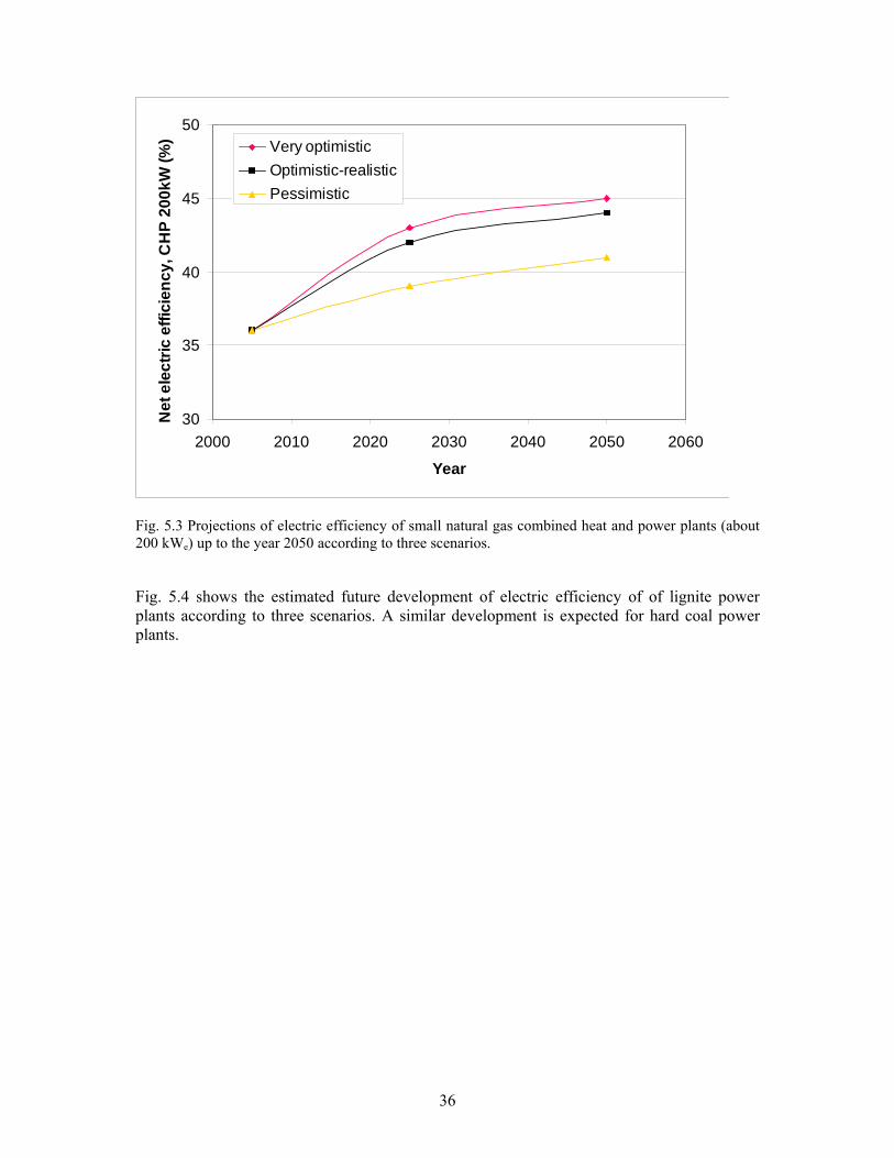
Fig. 5.3 shows the future development of small natural gas combined heat and power plants as assumed in the three scenarios.

36

30

35

40

45

50

2000 2010 2020 2030 2040 2050 2060

Year

Net

ele

ctric

effi

cien

cy, C

HP

200k

W (%

) Very optimisticOptimistic-realisticPessimistic

Fig. 5.3 Projections of electric efficiency of small natural gas combined heat and power plants (about 200 kWe) up to the year 2050 according to three scenarios.

Fig. 5.4 shows the estimated future development of electric efficiency of of lignite power plants according to three scenarios. A similar development is expected for hard coal power plants.

37

0

10

20

30

40

50

60

2005 2025 2050

elec

tric

net

effi

cien

cy, l

igni

te p

ower

pla

nt [%

]

pessimisticrealistic-optimisticvery optimistic

Fig. 5.4 Projections of net electric efficiency of lignite power plants up to the year 2050 according to three scenarios.

5.1.3 Combination of spatial and temporal parameters

LCA results of Carbon Capture and Storage (CCS) technologies can depend on both spatial and temporal parameters: As indicated above, distance of CO2 transport and the depth of the storage site (spatial) as well as the reference year for the assessment (temporal) have an impact on LCA results. Such dependencies are illustrated in Fig. 5.5 and Fig. 5.6 for cumulative greenhouse gas (GHG) emissions of hard coal chains with and without CCS (in each graph, the red line “CO2 T&S” represents the total cumulative GHG emissions with CCS). Fig. 5.5 represents the minimum of achievable CO2 reductions for hard coal chains with CCS until year 2050 (pessimistic scenario, post-combustion capture, CO2 storage at a depleted gas field with a depth of 2500 m), Fig. 5.6 the maximum (very optimistic scenario, oxyfuel combustion capture, CO2 storage at a saline aquifer with a depth of 800 m). The relevance of both spatial and temporal parameters are obvious: technological advancements will allow not only increasing power plant efficiencies, but also reduced energy demand for CO2 capture; the contributions from CO2 transport and storage (“T&S”) depend very much on the storage option.

38

0.0

0.1

0.2

0.3

0.4

0.5

0.6

0.7

0.8

0.9

2005-2010 2025 2050

kg (C

O2-

eq) /

kW

h

PC w/o CCS maxCoal supplyPP operationPP InfrastructureCO2 T&S

Hard Coal PCw/o & with CO2

Post-combustionCapture

PCw/CCS

Reduction: 68%

Reduction: 63%

Fig. 5.5 Projections of cumulative GHG emissions from hard coal PC power plants with post combustion capture and CO2 storage at a depleted gas field up to the year 2050 according to the pessimistic scenario (with CCS: additive emissions from the different steps in the energy chain – the red line represents the total emissions with CCS).

0.0

0.1

0.2

0.3

0.4

0.5

0.6

0.7

0.8

0.9

2005-2010 2025 2050

kg (C

O2-

eq) /

kW

h

PC w/o CCS minCoal supplyPP operationPP InfrastructureCO2 T&S

Hard Coal PCw/o & with CO2

Oxyfuel-combustionCapture

PCw/CCS

Reduction: 84%Reduction: 81%

Fig. 5.6 Projections of cumulative GHG emissions from hard coal PC power plants with oxyfuel combustion capture and CO2 storage at a saline aquifer up to the year 2050 according to the very optimistic scenario (with CCS: additive emissions from the different steps in the energy chain – the red line represents the total emissions with CCS).

39

5.2 Bioenergy Section 5.2.1 shows an overview on important spatial parameters of bioenergy systems. Section 5.2.2 discusses temporal parameters for bioenergy.

5.2.1 Spatial parameters

5.2.1.1 List of parameters

The following key parameters of bio-energy production depend strongly on the location (Gärtner 2006):

• Yield of crops and potential of available agricultural area

• Potential of available biomass residues

Except for fuel production, the space-dependencies of parameters for thermal biomass power plants are essentially very similar to those for thermal fossil power plants.

Regulation dependency

For some very small combustion devices, there are currently either no or at least no binding uniform regulations for the whole of Europe. Nevertheless, the emissions from small combustion devices can be rather significant. Recently, the German Umweltbundesamt estimated that the total PM10 emission from small wood combustion plants in Germany have been approximately as high as the total PM10 emissions from the motors of passenger cars, trucks and motor cycles (without PM10 emissions due to abrasion and road dust). The annual PM10 emission from Germany’s small wood combustion plants have approximately doubled since 1995 reaching about 24 kt/year in 2003 compared to 22.7 kt/year from motors used for road transport (UBA 2006). Fine particulates are an important cause of human health damages related to air emissions from energy systems and thus have strong influence on external costs. The health effects due to PM10 emissions from small wood combustion sources are strongly dependent on the location. In highly populated areas the damages per unit of PM10 emitted are high because of the large number of people affected. Currently, there are no legal emission limits for particulate emissions from small wood combustion plants below 15 kW in Germany (UBA 2006). Due to the increasing particulate emissions, wood combustion systems are now under scrutiny. Because of the strong space-dependency of the effects, local emission regulations for small combustion plants might be expected in the near future.

5.2.1.2 Geographical reference data related to system parameters

The following table Tab. 5.2 gives an overview on proposed geographical reference data that might be used to characterize the space-dependency of important system parameters of biomass systems.

40

Tab. 5.2 Proposed geographical reference data for selected spatial parameters of biomass energy (Gärtner 2006).

System Geographical reference data Data available at

For parameter(s)

Biomass Climate zone, average summer temperature

Altlas, encyclopedia

Energy crop yield (MJ/ha)

Mean annual precipitation (mm/a) (in combination with climate zone)

Atlas, encyclopedia

Irrigation needs (mm/yr), energy crop yield (MJ/ha)

Area/regional soil characteristics (Geological) atlas

Irrigation needs (mm/yr), energy crop yield (MJ/ha)

Annual net production of cereals Statistical databases

Residual biomass availability (MJ/year)

Annual consumption of domestic wood in the wood industry

Statistical databases

Residual biomass availability (MJ/year)

Annual forest growth Statistical databases

Residual biomass availability (MJ/year)

Soil characteristics may influence the energy crop yield strongly in an area or region. However, their influence on the average yield in a large country is small due to different soil types throughout within the country.

There is a certain correlation between the climate zone and the mean annual precipitation. All other parameters specified are assumed to be independent from each other.

5.2.1.3 Steps towards quantification

Biomass yield

A rough mathematical function showing the dependency of the energy crop yield may be (Gärtner 2006)

Yield = A × (average summer temperature – B) × available water – C

with A, B, and C being variable in time due to plant breeding success. The validity of this function is given in a certain temperature and water range.

Residual biomass availability

A rough mathematical function showing the dependency of straw available from the cereals may be (Gärtner 2006)

Availability of straw = A × cereal production – B

with A and B being variable in time due to plant breeding success (aiming to increase the grain/straw ratio). The validity of this function is given in a certain temperature and water range.

41

Likewise, a rough mathematical function can be derived showing the dependency of the residual forest wood availability (Gärtner 2006):

Availability of res. forest wood = A × dom. wood consumption + B × forest growth

with A and B being constant.

5.2.1.4 Conclusions on the space-dependency of life cycle results

Partly: yield of energy crops influences directly the land use for bio-energy systems. Other life cycle results may be influenced by yield or residual crop availability to a smaller extent, e.g. changes due to transport distances or field work being necessary likewise with high or low yield. For this, no clear relation can be given. Generally, higher yields or higher residue availability may diminish the life cycle results. However, if higher yields are reached by irrigation, this generally provokes higher fossil energy consumption and higher emissions.

5.2.2 Time-dependent parameters

Key parameters which are important to describe the changes of bio-energy systems in future (Gärtner 2006):

• Plant breeding: bio-energy crop yield

• Nitrogen fertiliser production: efficiency and emissions

• Fertiliser application technique: emissions from the field

• Conversion plant: efficiency and emissions

• Water availability

Quantitative estimates of the future development of the first four parameters in the list are discussed in the corresponding NEEDS report (Gärtner 2007a). Possible changes of water availability in future have not been investigated within the NEEDS project.

Scenario dependency of the parameters (Gärtner 2007b):

• Parameters independently changing in all scenarios:

• Fertiliser production

• Fertiliser application

• Combustion emissions: CO, PM, NOx

• Parameters dependent on the scenarios:

• Yield of energy crops

• Combustion efficiency

• Combustion emissions (others)

Specific points on scenario dependency:

• Plant breeding: bioenergy crop yield – depends to a certain extent on the area cultivated with the bioenergy crop (i.e. on the scenario).

• Nitrogen fertiliser production: efficiency and emissions. The production of nitrogen fertiliser currently requires large amounts of fossil fuels. It is assumed that also in future fossil fuel needs will be substantial so that CO2 emissions associated with

42

nitrogen fertilizer production will remain significant. Reductions of ammonia emissions for nitrogen fertiliser production are likely in future (Gärtner 2008).

• Fertiliser application technique: emissions from the field – depend on the scenario.

• Conversion plant: efficiency and emissions – depend on the scenario.

The following parameters are most likely approximately constant and can be used as a stable basis for LCA assessment:

• Bioenergy crops: machinery work for field preparation, fertilising, harvest, storage can be assumed to be constant.

• Bioenergy crops and residual biomass: auxiliary materials for the conversion/combustion process can be assumed to be constant.

Conclusions on the time-dependency of life cycle results:

• Plant breeding: bioenergy crop yield – when rising with a constant demand for irrigation leads to slightly lower LCI results.

• Nitrogen fertiliser production: increasing efficiency and decreasing emissions leads to lower LCI results

• Fertiliser application technique: decreasing emissions from the field lead to lower LCI results

• Conversion plant: increasing efficiency and decreasing emissions leads to lower LCI results.

Space dependency changing with time:

• Probably, climate change will influence yield of crops and necessity of irrigation within single regions and thus the distribution of yield all over Europe.

• Development of water availability can be different for different countries as climate is supposed to lead to both increasing or decreasing precipitation depending on the location.

The model results recently published by the IPCC predict significant changes of crop yields in Europe due to climate change (IPCC 2007). The IPCC expects that crops show a northward expansion in area by the mid of the 21st century. “The greatest increases in climate-related crop yields are expected in northern Europe (e.g., wheat: +2 to +9 % by 2020, +8 to +25 % by 2050, +10 to +30 % by 2080), while the largest reductions are expected in the south (e.g., wheat: +3 to +4 % by 2020, −8 to +22 % by 2050, −15 to +32 % by 2080).” (IPCC 2007)

Climate change is also expected to influence forests and thus availability of wood bio-energy. “Forested area is likely to increase in the north and decrease in the south. A redistribution of tree species is expected, and an elevation of the mountain tree line. Forest-fire risk is virtually certain to greatly increase in southern Europe.” (IPCC 2007).

In the NEEDS biomass report (Gärtner 2007a), biomass potentials for energy crops and forestry and residues are estimated for the years 2005, 2025, and 2050. Future biomass usage for electricity in the EU-28 is outlined. Size, electrical efficiency, thermal efficiency, life time, electricity production, full load hours, PM10 emissions, and CO emissions of future

43

bioenergy CHP plants are estimated. Yield, bulk density, moisture at harvest, moisture at combustion / gasification, LHV at combustion/gasification, and ammonia emissions from field are estimated for different future biomass production schemes (short rotation poplar, wheat straw, residual forest wood, short rotation poplar, wheat straw, residual forest wood). Future costs of steam turbines and gasifiers for biomass energy are estimated (Gärtner 2007a).

5.3 Photovoltaics Key parameters for LCA of photovoltaics as investigated within the NEEDS project are (Frankl 2005):

• Module efficiency

• Module lifetime

• Material resource consumption

• kg/Wp of semiconductor feedstock

• Energy resource consumption

• kWhel/Wp of semiconductor feedstock

• kg/Wp of fuels

• BOS performance ratio in function of

• Application

• Location

5.3.1 Spatial parameters

First of all, the annual electricity production of photovoltaic cells depends on the direct solar normal irradiation (in kWh/(m2*a)) and on the efficiency of the chosen PV technology.

PVGIS provides web-based interactive applications (http://re.jrc.ec.europa.eu/pvgis/) showing monthly and yearly values of global irradiation per square meter and of electricity production from a given system (Šúri et al. 2007). The database has a resolution of 1 km x 1km. A map of the yearly sum of global irradiation in Europe is shown in Fig. 4.9.

Another possible source of solar irradiation data is the SOLEMI database (www.solemi.de).

Space dependency of LCA results, example: For PV, assumed that the life time of the plant does not depend on the location (which might be doubtful for extreme weather conditions), typical life cycle results like CO2 kg/kWhe are inversely proportional to the local annual solar irradiation on an optimally-oriented PV module (up to the temperature correction discussed below).

The efficiency of photovoltaic cells depends on the PV technology but to a certain extent also on the temperature of the modules. The solar irradiation heats up the module. This results in a reduction of the efficiency. The efficiency loss depends on the type of solar cells. Fig. 5.7. illustratively shows the approximate dependency of the efficiency on the module temperature for different PV types.

Measurements in Germany have shown that the loss of annual electricity production from PV modules can be 7.5% to 10% due to temperature effects alone (Eicker 2003). In the study, PV systems cooled by back-ventilation of facades have been compared to non-back-ventilated systems. The positive effect of a low ambient temperature on efficiency compensates a little

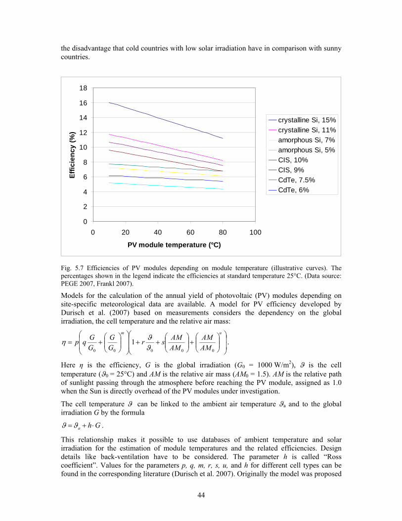
44

the disadvantage that cold countries with low solar irradiation have in comparison with sunny countries.

0

2

4

6

8

10

12

14

16

18

0 20 40 60 80 100

PV module temperature (°C)

Effic

ienc

y (%

)

crystalline Si, 15%crystalline Si, 11%amorphous Si, 7%amorphous Si, 5%CIS, 10%CIS, 9%CdTe, 7.5%CdTe, 6%

Fig. 5.7 Efficiencies of PV modules depending on module temperature (illustrative curves). The percentages shown in the legend indicate the efficiencies at standard temperature 25°C. (Data source: PEGE 2007, Frankl 2007).

Models for the calculation of the annual yield of photovoltaic (PV) modules depending on site-specific meteorological data are available. A model for PV efficiency developed by Durisch et al. (2007) based on measurements considers the dependency on the global irradiation, the cell temperature and the relative air mass:

⎟⎟

⎠

⎞

⎜⎜

⎝

⎛⎟⎟⎠

⎞⎜⎜⎝

⎛+⎟⎟

⎠

⎞⎜⎜⎝

⎛++

⎟⎟

⎠

⎞

⎜⎜

⎝

⎛⎟⎟⎠

⎞⎜⎜⎝

⎛+=

um

AMAM

AMAMsr

GG

GGqp

00000

1ϑϑη .

Here η is the efficiency, G is the global irradiation (G0 = 1000 W/m2), ϑ is the cell temperature (ϑ0 = 25°C) and AM is the relative air mass (AM0 = 1.5). AM is the relative path of sunlight passing through the atmosphere before reaching the PV module, assigned as 1.0 when the Sun is directly overhead of the PV modules under investigation.

The cell temperature ϑ can be linked to the ambient air temperature ϑa and to the global irradiation G by the formula

Gha ⋅+=ϑϑ .

This relationship makes it possible to use databases of ambient temperature and solar irradiation for the estimation of module temperatures and the related efficiencies. Design details like back-ventilation have to be considered. The parameter h is called “Ross coefficient”. Values for the parameters p, q, m, r, s, u, and h for different cell types can be found in the corresponding literature (Durisch et al. 2007). Originally the model was proposed

45

in order to select the most appropriate PV module type for a specific site based on estimates of costs and electricity yield because different PV technologies have different seasonal characteristics of performance i.e. there might be modules more suited to particular climates. Variations of the model have been proposed elsewhere (Durisch et al. 2006).

An integration of a parameterised model of PV efficiency as function of global irradiation and temperature into LCA modelling would be relatively straightforward.

Modelled GIS data of temperatures in Europe are provided for example by PVGIS (http://re.jrc.ec.europa.eu/pvgis/) or by meteorological institutes.

The area potential for PV on roofs and facades of buildings is listed in the NEES report on PV (Frankl et al. 2007) for different countries of the world categorized according to building classes (residential buildings, agricultural buildings, industrial buildings, commercial buildings, other buildings). A map shows the energy potential from PV around the world (kWh/m2) (Frankl et al. 2007).

5.3.2 Time-dependent parameters

The cumulative installed PV capacity for different applications (grid-connected, off-grid) from 1992 to 2003 is shown in the NEEDS report on PV technology (Frankl et al. 2007). The yearly installed new PV capacity is shown from 1990 to 2004. The future PV capacity installed up to 2050 both in the OECD Europe and worldwide is estimated in 10-years steps up to 2050.

Average yearly growth rate, installed capacity, market share OECD Europe/World total, electricity production, application market share up to 2050 are estimated. Capacity production for PV market segments is estimated up to 2030.

A cost experience curve of PV modules from 1976 to 2001 is shown. Projections of PV module costs (Euro/Wp) until 2050 are shown for learning rates between 0.1 and 0.3 and for market growth rates between 10% and 20%. Projections of electricity production costs (Euro/kWh) and projections of improvements of PV cell efficiency for various technologies are shown. For the year 2050, estimates of module efficiency and module lifetime are shown for various PV cell types (Wafer-based c-Si: Cz, Fz mc, ribbon; Thin films: CIS, CdTe, a-Si/µc-Si, thin Si films, Pin-ASI and ASI-THRU; New concept devices: Ultra-high efficiency (3rd generation, Quantum wells Nanostructures Concentrators), Ultra-low cost (Dye-sensitized cells, Organic cells)). The development of PV technology market shares is estimated until 2050. Cumulative installed capacity, average efficiency, module lifetime, investment costs and PV electricity costs are estimated for present, 2025, and 2050. Projections of average cost of Power Plant size PV are shown as functions over time from 2004 to 2050 (Frankl et al. 2007).

5.4 Solar thermal power In section 5.4.1, important spatial parameters related to solar thermal power are shown. Section 5.4.2 discusses temporal parameters for solar thermal power.

46

5.4.1 Spatial parameters

5.4.1.1 List of parameters

The following key parameters for solar thermal power plants depend significantly on the location (Viebahn 2006):

• Annual electricity generation (yield in kWhe/y per installed kWp) and therefore the solar full load hours (h/y) and the LEC (levelised electricity costs).

• LEC depend not only on the annual electricity generation but also on the electricity transport distance and therefore the power plants’ location (even if the solar irradiation of Germany and Egypt was the same, solar electricity transported from Egypt would costs 1 to 1.5 ct/kWh,e more than produced in Germany).

• LCA results of materials used for constructing the power plants (steel, concrete, glass) (different production conditions in Europe and in North Africa).

Parameter dependencies:

• Electricity transport distance depends on the location.

• Solar full load hours depend on the direct normal irradiation.

5.4.1.2 Geographical reference data related to system parameters

Tab. 5.3 gives an overview on proposed geographical reference data that might be used to characterize the space-dependency of important system parameters of biomass systems.

Tab. 5.3 Proposed geographical reference data for selected spatial parameters of solar thermal power (Viebahn 2006).

System Geographical reference data Data available at For parameter(s)

Solar thermal

Solar direct normal irradiation (in kWh/m2,y or in W/m2,y)

SOLEMI database (www.solemi.de)

DNI (direct normal irradiation)

Natural gas price in case of hybrid systems

Energy related databases

Fuel price

5.4.1.3 Steps towards quantification

The following relations may be used in an LCA system for an approximate space-dependent quantification of the electricity production from solar thermal plants (Viebahn 2006):

47

E = DNI * SF * η

with E electricity production in kWh,el/y DNI direct normal irradiation in kWh/m2,y SF solar field (solar collector) in m2 η efficiency (= solar efficiency times power unit’s efficiency)

or alternatively

E = P * sfh

with E = electricity production in kWh,el/y P = installed capacity in kW,el sfh = solar full load hours.

Concerning space- and time-dependency, in the NEEDS technology reports on solar thermal power, monthly electricity yields and full load hours per year depending on site specific irradiation are shown (Viebahn & Lechón 2007). Future high voltage direct current transmission lines for transport of solar thermal electricity from Northern Africa to Europe are proposed and corresponding transport distances are estimated (Viebahn et al. 2008).

5.4.1.4 Conclusions on the space-dependency of life cycle results

LCA results for solar thermal power plants linearly depend on the solar direct irradiation and therefore on the location.

5.4.2 Time-dependent parameters

The following key parameters are important to describe the changes of solar thermal power plants in future:

• Capacity of thermal storage (influences the number of solar full load hours). • Efficiency.

Scenario dependency of the parameters:

Both parameters (development of thermal storages as well as efficiency) depend strongly on scenarios.

The technical lifetimes of materials are most likely approximately constant over time.

In the NEEDS technology reports on solar thermal power, projections of the installed capacity of for solar thermal power plants, solar thermal electricity production and full load hours up to year 2050 are shown (Viebahn & Lechón 2007, Viebahn et al. 2008).

Future investment costs, storage capacity, and electricity generation costs for a hybrid power plant are shown. Projections of full load hours, power transmission costs, solar share, solar full load hours, storage capacity are shown for 2005 to 2050.

Experience curves projections for investment costs for collector field, power block & BOP & Adaptation, and storage depending on estimated future installed solar thermal capacity are provided. The principle problem of constructing simple learning rates for future thermal solar power plants costs is critically discussed (Viebahn & Lechón 2007). Nevertheless, a learning

48

rate leading to a simple parameter description of costs could be possibly constructed for the time period after 2020 when the solar thermal power plants are fully developed and running in a solar only mode reaching maximum solar full load hours (Viebahn & Lechón 2007).

Future total solar thermal electricity generation cost as functions of time between 2000 and 2050 are shown. Learning rates for storage system (about 12%), collector field (about 12%), and power block/BOP (about 5%) are discussed. Future size, electrical efficiency, life time, solar share and costs are estimated (Viebahn & Lechón 2007).

The concept of learning curves is also extended in a way to “material learning curves” for solar thermal power plants. The material reduction development curves as functions of time starting at the present technologies and depending on the three technology development scenarios are constructed (Viebahn et al. 2008).

5.5 Wind An important set of parameters for the life cycle assessment of wind power are the masses of materials needed for the plant. Another important parameter is the average wind speed in order to estimate the annual electricity production of the plant at a given location.

Within the DOWEC project (DOWEC 2003), design models for wind power plants have been developed. The models estimate for example the masses of different components of the wind plant like the turbines or the tower. Parameters considered are for example the electric power, the wind speeds and the depth of water for offshore wind plants. Such design models could be possibly used to calculate the material needs for a parameterised LCA model for wind power plants.

As an example, Fig. 5.8 shows the total mass of the tower as a function of the water depth for a 3 MW turbine of an offshore wind power plant.

Fig. 5.8 Mass of the tower as a function of the water depth for three offshore tower concepts for a 3 MW wind turbine with a hub height of 60 m (Source: Zaaijer 2001).

Liu et al. (2008) have derived a global offshore wind power map based on measurements by a space-based radar. The data has been collected over a period of eight years. The wind potential is shown as wind power density in W/m2.

49

As mentioned above, the local wind and wave conditions have also influence on the design and thus on the material needs of an offshore wind power plant because the stability has to be guaranteed considering also extreme wind speeds and extreme waves during the lifetime.

Climate change might influence the wind speeds and spatial distribution of future wind power. In case of more frequent storms, the shut down frequency might increase as well.

The NEEDS wind report provides the development of the rotor diameter of wind turbines as function of time since 1985 (Hassan et al. 2007). Projections for global wind power production and wind power capacity up to year 2050 are provided. The future share of off-shore wind power in total wind power capacity is estimated. Averages sizes of future wind turbines, bumbers of wind farms and average capacity of wind farms are projected. Further parameters estimated are height, length of blades and water depth for offshore wind turbines.

Experience curves for investment costs and water depth depending on accumulated wind power capacity are shown (1990 to 2005); Future costs are estimated (Hassan et al. 2007).

5.6 Hydrogen Hydrogen is not a primary energy source but only an energy carrier which has to be produced. Thus the production conditions are most important. Concerning the spatial aspect, the future transport and distribution network is relevant for LCA. In case of transport via pipelines, a GIS-based LCA system would be advantageous similarly like for new methane pipelines. Important LCA parameters are leakage rates for transport and storage of hydrogen.

The NEEDS report on hydrogen power shows possible future pathways for hydrogen imports to Europe based on the Encouraged project (Maack 2007).

Future shares of hydrogen vehicles and shares of hydrogen driven micro CHP in households for 2010, 2020, 2030, 2040, and 2050 are shown. Annual operating hours, lifetime (20a), annual hydrogen production, efficiency electricity-hydrogen (70%), and costs for electrolysis in 2020 are estimated (Maack 2007).

5.7 Fuel cells The fuel cell technology does not depend very much on spatial parameters. The essential factor is the future development of the technology.

Installed capacity of large fuel cells, per annum and cumulative, number of installed units, and cumulative capacity of small stationary fuel cells between 1996 and 2006 are shown in the NEEDS report on fuel cells (Gerboni et al. 2007). Percentages of installations of fuel cell types between 2003 and 2006 are presented.

Projection curves for global stationary fuel cell capacity are shown up to year 2050. The report refers to learning curves from the WETO report (EU (2003) – “World energy, technology and climate policy outlook 2030 – WETO”, Download from ec.europa.eu/research/energy/pdf/weto_final_report.pdf). Investment costs of fuel cells for 2005, 2025, and 2050 are estimated based on progress ratios between 0.7 and 0.9. Net electric power, net thermal power, electric efficiency, thermal efficiency, technical life time [a] of stack, technical life time of BoP and costs are estimated up to 2050 for different fuel cell types (SOFC, SOFC CHP, PEMFC, MCFC, Hybridised MCFC) (Gerboni et al. 2007).

50

5.8 Nuclear For the LCA of nuclear power, the mining, milling and enrichment of uranium are relatively important. The energy requirements and the LCA burdens for the fuel production from natural ore depend on the concentration of uranium in the ore. For future nuclear power, uranium reservoirs with lower uranium concentration compared to current mines have to be taken into consideration. The uranium concentration of ore should be considered for parameterisation.

Local conditions play a role for the LCA of uranium tailings. Climatic conditions are important for the different likely weathering patterns of the mill tailings and their effects on the radon flux (Dones et al. 2005).

Technical lifetime, construction time, decommission share and cost data for nuclear power plants in 2005, 2025, and 2050 are provided in the NEEDs report for nuclear power (Lecarpentier & Lecointe 2007). Future fuel cycle costs are estimated.

5.9 Wave and tidal power Concerning space-dependency, the country-specific wave energy potentials (kW/m) near shore at the west coast of Europe and the potentials along the coasts of the world are shown in the NEEDS report on wave and tidal power (Sørensen et al. 2007). The highest wave activity (kW/m) is found between the latitudes of ~30o and ~60o on both hemispheres.

For tidal energy, the tidal range in meters is shown on a world map (Sørensen et al. 2007).

Future projections of installed capacity deployment are estimated (Sørensen et al. 2007).

5.10 Hydropower Hydropower plants have not been investigated in NEEDS RS1a. In fact, most likely only few changes of technical parameters may be expected in future because the efficiency of hydro power plants is already very high. Modern hydro power plants can reach an efficiency of about 90% so that the margins for further improvements are small. A field of active research is the extension of lifetime of turbines (e.g. Escaler et al. 2006) which would improve the overall LCA performance.

Nevertheless, future changes of the hydro cycle due to climate change might have an impact on hydropower production. Changes of the hydro power potential can have significant influence on LCA results and external costs of the electricity mix. Hydro power plants in Europe have relatively low environmental impacts in terms of external costs according to current external cost methodology. Thus a higher share of hydropower usually implies lower external costs of the electricity mix (keeping all other systems constant).

According to recent results of climate change modelling, significant changes of the hydro power production in Europe are possible. “By the 2070s, hydropower potential for the whole of Europe is expected to decline by 6%, with strong regional variations from a 20 to 50% decrease in the Mediterranean region to a 15 to 30% increase in northern and eastern Europe.” (IPCC 2007). A negative influence on life cycle burdens and external costs of the European electricity mix can be expected in particular if hydropower had to be replaced by fossil power plants which have usually much higher external costs compared to hydro power plants.

The development of LCA and LCIA results for the future electricity mix thus depends also on the assumed emission scenario and the resulting change of the hydro cycle. A

51

parameterization and a coupling to climate change models would be advantageous for the simulation of the future electricity mix within LCA. Local changes of precipitation due to climate change under different scenario assumptions have been studied for example in Jacob et al. (2008) for Germany until year 2100 on a 10 km x 10 km grid.

52

6 Conclusions

Within this work package of the NEEDS project, a general framework of a parameterisation methodology for life cycle analysis of energy systems has been developed.

Several explicit examples for time-dependency, space-dependency and technology-dependency of LCA parameters are provided and discussed. For different advanced electricity generation systems, sets of relevant space- and time-dependent parameters have been collected (partly quantitatively and partly qualitatively).

The increasing complexity of the LCA databases is difficult to handle. Moreover, extending the datasets in space and time, while keeping control over consistency and correctness, becomes more and more difficult. Parameterisation can help to facilitate the further extension of LCA modelling towards larger spatial coverage, more sophisticated spatial differentiation and future scenarios. A high spatial differentiation of LCI data is desirable when the LCI model is coupled to environmental impact and external costs assessment.

General aspects of an advanced parameterised LCA system have been discussed. It has been proposed that the connection of the LCA model to a Geographical Information System (GIS) should be considered because several spatial parameters can be treated systematically in a GIS software.

The possibility and appropriateness of parameterisation depend much on the specific energy system, in particular for the space-dependency. There is no common simple approach for general spatial parameterisation; every issue has to be investigated separately.

The time series related to three future scenarios developed within the LCA stream RS1a of the NEEDS project provide a useful basis for the time-dependent parameterisation.

We have also discussed the possibility to generalise the experience curve method known from economy to environmental experience curves for the parameterisation of the future development of energy systems. Few examples have been derived explicitly. The generalisation of the experience curve approach to environmental burdens opens an interesting possibility for the modelling of future scenarios. Nevertheless, the approach has to be handled with care because the influence of political decisions on emission limits may have a more erratic impact on the development of environmental burdens than the permanent pressure of the market has on reductions of costs. It can also be concluded that external costs, contrary to internal costs, cannot be expected to follow a simple experience curve approach in general although it might be the case for some technologies and certain time periods.

In view of the large number of parameters used in state-of-the-art LCA modelling, it was far beyond the scope of this work package to cover systematically all parameters. The focus of the present work was more on the variety of parameters that have to be considered rather than completeness. The implementation of the proposed methods up to a running advanced LCA model would require deeper investigations of single energy systems and background processes and need substantial resources. But especially spatial differentiation leads to a big increase of the amount of data. Therefore, even a limited reduction by partial parameterisation is helpful. Thus it would be recommendable to consider a step-wise and iterative implementation of parameterisation into LCA modelling.

53

7 References

Amann et al. (2005). Amann M., Imrich Bertok I., Cofala J., Gyarfas F., Heyes C., Klimont Z., Schöpp W. and Winiwarter W. (2005) Baseline Scenarios for the Clean Air for Europe (CAFE) Programme. International Institute for Applied Systems Analysis (IIASA), Laxenburg, Austria, retrieved from: http://europa.eu.int/comm/environment/air/cafe/general/pdf/cafe_lot1.pdf.

Bachmann R. (2004). Fossil – Thermische Kraftwerke. The Energy Consulting Group Ltd. Energieperspektiven. Bundesamt für Energie. Bern.

Barreto L. (2001) Technological Learning In Energy Optimisation Models And Deployment Of Emerging Technologies. DISS. ETH Nr 14151.

Böge A. (1999). Das Techniker-Handbuch. Vieweg. Braunschweig.

Boyce M.P. (2002). Handbook for cogeneration and combined cycle plants. ASME Press, New York.

Boyce M.P. (2006) Gas turbine engineering handbook. GPP, Boston.

Brückner-Kalb J. R. (2008). Sub-ppm-NOx–Verbrennungsverfahren für Gasturbinen. Dissertation, Technische Universität München, Institut für Energietechnik.

Claeson Colpier U. and Cornland D. (2002) The economics of the combined cycle gas tur-bine - an experience curve analysis. Energy Policy 30 pp. 309-316.

Dones et al. (2005). R Dones, T Heck, M Faist Emmenegger and N Jungbluth. Int J LCA 10 (1) 10 – 23.

Dones et al. (2007). Roberto Dones, Christian Bauer, Thomas Heck, Oliver Mayer-Spohn, Markus Blesl. Deliverable n° T7.4 - RS1a, “Technology report: Advanced fossil energy”. NEEDS (New Energy Externalities Developments for Sustainability), European Commission.

DOWEC (2003). Dutch Offshore Wind Energy Converter (DOWEC) project. www.ecn.nl/en/wind/additional/special-projects/dowec.

Durisch et al . (2006). W. Durisch, K.-H. Lam and J. Close. Efficiency and degradation of a copper indium diselenide photovoltaic module and yearly output at a sunny site in Jordan. Applied Energy, Volume 83, Issue 12, December 2006, Pages 1339-1350

Durisch et al . (2007). W. Durisch, B. Bitnar, J.-C. Mayor, H. Kiess, K.-H. Lam, and J. Close. Efficiency model for photovoltaic modules and demonstration of its application to energy yield estimation. Solar Energy Materials & Solar Cells 91 (2007) 79–84.

DWTC (2001) Coal options. Report. Federal Office for Scientific, Technical and Cultural Affairs (OSTC/DWTC), Brussels. www.belspo.be/belspo/home/publ/ pub_ostc/CG2131/rCG23_en.pdf

ECLIPSE (2004). http://88.149.192.110/eclipse_eu/index.html

Eicker U. (2003). Solar Technologies for Buildings. Wiley 2003.

Escaler et al. (2006). X Escaler, E Egusquiza, M Farhat, F Avellan, M Coussirata. Detection of cavitation in hydraulic turbines. Mechanical Systems and Signal Processing 20 (2006) 983–1007.

European Commission (2005) Externalities of Energy: Extension of accounting framework and Policy Applications (ExternE-Pol). Vol. Final Report, Contract ENG1-CT2002-00609.

54

European Commission, DG Research, Technological Development and Demonstration (RTD), Brussels, www.externe.info/expoltec.pdf.

Frankl (2005), Presentation NEEDS RS1a Fontainbleau 15_16 Nov 2005.

Frankl et al. (2007). Paolo Frankl, Emanuela Menichetti and Marco Raugei with contributions by Simona Lombardelli and Giacomo Prennushi. Technical paper n° 11.4 - RS Ia “Report on technical specification of reference technologies (Photovoltaic systems)”. NEEDS (New Energy Externalities Developments for Sustainability), European Commission.

Gärtner (2006). Sven Gärtner. Answers to questionnaire in NEEDS RS1a WP4. IFEU.

Gärtner (2007a). Sven Gärtner. Technical paper n° 13.4 - RS 1a, “Technology report: biomass and bioenergy technologies”. NEEDS (New Energy Externalities Developments for Sustainability), European Commission.

Gärtner (2007b). Sven Gärtner. Presentation NEEDS, CIEMAT, Madrid, 2 – 3 October 2007.

Gärtner (2008). Sven Gärtner . Deliverable n° 13.2 - RS 1a, “Final report on technical data, costs and life cycle inventories of biomass CHP plants”. NEEDS (New Energy Externalities Developments for Sustainability), European Commission.

General Electric (2001). Next Generation Gas Turbine (NGGT) Systems Study. Final report for US DOE. Morgantown. www.osti.gov/bridge/servlets/purl/791498-4O5Tvo/native/791498.pdf.

Gerboni et al. (2007). Raffaella Gerboni, Martin Pehnt, Peter Viebahn, Evasio Lavagno. Technical paper n° 9.4 - RS Ia, “Technology report on fuel cells”. NEEDS (New Energy Externalities Developments for Sustainability), European Commission.

Hassan et al. (2007). Abdi Ashur Hassan, Kim Winther and Henriette Hassing Corlin. Deliverable T 10.04 - RS 1a - WP10 “Roadmap for offshore wind”. NEEDS (New Energy Externalities Developments for Sustainability), European Commission.

Heck (2004). Heck T., Wärme-Kraft-Kopplung. In: Sachbilanzen von Energiesystemen: Grundlagen für den ökologischen Vergleich von Energiesystemen und den Einbezug von Energiesystemen in Ökobilanzen für die Schweiz (Ed. Dones R.). Final report ecoinvent 2000 No. 6, Paul Scherrer Institut Villigen, Swiss Centre for Life Cycle Inventories, Duebendorf, CH, Vo.6-X, Online-Version under: www.ecoinvent.ch.

Jacob et al. (2008). Daniela Jacob, Holger Göttel, Sven Kotlarski, Philip Lorenz, Kevin Sieck. Klimaauswirkungen und Anpassung in Deutschland – Phase 1: Erstellung regionaler Klimaszenarien für Deutschland. Max-Planck-Institut für Meteorologie (MPI-M), Hamburg. (www.umweltdaten.de/publikationen/fpdf-l/3513.pdf).

Lecarpentier & Lecointe (2007). David Lecarpentier, Claire Lecointe. Technical Paper T 14.4 – RS 1a, “Technology report: nuclear power plants”. NEEDS (New Energy Externalities Developments for Sustainability), European Commission.

Liu W. T., W. Tang, X. Xie (2008), Wind power distribution over the ocean, Geophys. Res. Lett., 35, L13808, doi:10.1029/2008GL034172.

Maack (2007). Maria Maack. Deliverable n° 8-4 RS1a, Generation, storage and distribution systems for the energy carrier HYDROGEN. NEEDS (New Energy Externalities Developments for Sustainability), European Commission.

Pauls P. (2003). Siemens Press Release. Reference Number: PG 200310.002 e, Press Office Power Generation, Siemens AG, Munich, Germany.

55

PEGE (2007) Temperaturkoeffizienten. wohnen.pege.org/2005-photovoltaik/temperaturkoeffizient.htm

IEA (2004). World Energy Outlook 2004. International Energy Agency, Paris.

IPCC (2007). IPCC Fourth Assessment Report: Climate Change 2007. Intergovernmental Panel on Climate Change. www.ipcc.ch.

Sørensen et al. (2007). Hans Chr. Sørensen, Lars Christensen, Stefan Naef. Deliverable n° 12.1 - RS Ia, “Report on technical specification of reference technologies (wave and tidal power plant)”. NEEDS (New Energy Externalities Developments for Sustainability), European Commission.

Šúri et al. (2007). Marcel Šúri, Thomas A. Huld, Ewan D. Dunlop, Heinz A. Ossenbrink. Potential of solar electricity generation in the European Union member states and candidate countries. Solar Energy 81 (2007) 1295–1305. http://re.jrc.ec.europa.eu/pvgis/.

Tehlar D. (2007). Status of combined heat and power (CHP) technology in Europe, Semesterarbeit, Paul Scherrer Institut, Villigen, Switzerland.

Tester et al. (2005). Tester J.W., Drake E.M., Golay M.W., Driscoll M.J., Peters W.A. Sustainable Energy. MIT Press, Cambridge MA.

UBA (2006). Die Nebenwirkungen der Behaglichkeit: Feinstaub aus Kamin und Holzofen, Umweltbundesamt, Dessau, 2006, www.umweltbundesamt.de/uba-info-presse/hintergrund/holzfeuerung.pdf

Viebahn (2006). Peter Viebahn. Answers to questionnaire in NEEDS RS1a WP4. DLR, Stuttgart.

Viebahn & Lechón (2007). Peter Viebahn, Yolanda Lechón Pérez. Technical paper n° 12.4 - RS Ia, “Technology report (including road mapping, tech-nology specification of current and future systems, development of costs) for solar thermal power plant technologies”. NEEDS (New Energy Externalities Developments for Sustainability), European Commission.

Viebahn et al. (2008). Peter Viebahn, Stefan Kronshage, Franz Trieb, Yolanda Lechon. Deliverable n° 12.2 - RS 1a, "Final report on technical data, costs, and life cycle inventories of solar thermal power plants". NEEDS (New Energy Externalities Developments for Sustainability), European Commission.

Zaaijer (2001). M.B. Zaaijer: Properties of offshore support structures for large scale wind turbines. Offshore Wind Energy Special Topic Conference, Brussels, Belgium, December 2001. http://www.lr.tudelft.nl/live/pagina.jsp?id=3dcbe092-4334-4d47-9f82-dff9ed15ab5e&lang=en&binary=/doc/EWEA_Offsh_Support.pdf