Synthetic Modeling for an Acoustic Exploration System for Physical Oceanography

BERTA BIESCAS,* BARRY RUDDICK,1 JEAN KORMANN,# VALENTÍ SALLARÈS,@

MLADEN R. NEDIMOVI�C,& AND SANDRO CARNIEL**

* Istituto di Scienze Marine, CNR, Bologna, Italy1Department of Oceanography, Dalhousie University, Halifax, Nova Scotia, Canada

# Barcelona Supercomputing Center, Barcelona, Spain@Department of Marine Geosciences, Institute of Marine Sciences, Barcelona, Spain&Department of Earth Sciences, Dalhousie University, Halifax, Nova Scotia, Canada

** Istituto di Scienze Marine, CNR, Venice, Italy

(Manuscript received 3 July 2015, in final form 9 November 2015)

ABSTRACT

Marine multichannel seismic (MCS) data, used to obtain structural reflection images of the earth’s sub-

surface, can also be used in physical oceanography exploration. This method provides vertical and lateral

resolutions ofO(10–100)m, covering the existing observational gap in oceanic exploration. All MCS data used

so far in physical oceanography studies have been acquired using conventional seismic instrumentation

originally designed for geological exploration. This work presents the proof of concept of an alternativeMCS

system that is better adapted to physical oceanography and has two goals: 1) to have an environmentally low-

impact acoustic source to minimize any potential disturbance to marine life and 2) to be light and portable,

thus being installed on midsize oceanographic vessels. The synthetic experiments simulate the main variables

of the source, shooting, and streamer involved in the MCS technique. The proposed system utilizes a 5-s-long

exponential chirp source of 208 dB relative to 1 mPa at 1m with a frequency content of 20–100Hz and a

relatively short 500-m-long streamer with 100 channels. This study exemplifies through numerical simulations

that the 5-s-long chirp source can reduce the peak of the pressure signal by 26 dBwith respect to equivalent air

gun–based sources by spreading the energy in time, greatly reducing the impact to marine life. Additionally,

the proposed system could be transported and installed in midsize oceanographic vessels, opening new ho-

rizons in acoustic oceanography research.

1. Introduction

The main physical parameters of the ocean (temper-

ature, salinity, pressure, and density) are traditionally

measured using vertical profiles as conductivity–

temperature–depth (CTD) casts or expendable bathy-

thermographs (XBT). These instruments sample the

ocean at a vertical resolution ofO(0.1–1)m, which allows

analysis of processes generated within the submesoscale

and finescale. However, this method of exploration does

not observe lateral structure at these scales because

typical lateral distances between vertical casts are

rarely shorter than O(103)m. This observational

gap is becoming increasingly relevant as numerical

models increase in resolution. Physical oceanographers

demand empirical data with a lateral resolution of

O(10–100)m to calibrate and validate new models and

theory (e.g., Ruddick 2003; Smith and Ferrari 2009; Hua

et al. 2013).

Marine multichannel seismic reflection (MCS) data,

collected and used to obtain structural images of the

earth’s subsurface, also display coherent reflections from

within the water layer. A partial list of features observed

via MCS data includes internal waves, thermohaline

staircases and intrusions, density and turbidity currents,

and submesoscale coherent vortices, which are key ocean

mixing processes (e.g., Biescas et al. 2008; Ménesguenet al. 2009; Pinheiro et al. 2010; Biescas et al. 2010;

Quentel et al. 2010; Vsemirnova et al. 2012; Holbrook

et al. 2013). Because of the signal redundancy provided

by the multiple illumination of a single reflector point,

MCS systems enhance coherent signals over noise, re-

sulting in clear acoustic images of the oceanic thermo-

haline structure with lateral and vertical resolutions of

Corresponding author address: Berta Biescas, Istituto di Scienze

Marine, CNR, Via Gobetti 101, 40129 Bologna, Italy.

E-mail: berta.biescas@ve.ismar.cnr.it

JANUARY 2016 B I E S CAS ET AL . 191

DOI: 10.1175/JTECH-D-15-0137.1

� 2016 American Meteorological Society

O(1–100)m. Furthermore, inversion methods applied to

acoustic images provide 2D temperature and salinity

maps, which may cover the current observational gap in

physical oceanography exploration (Papenberg et al.

2010; Bornstein et al. 2013; Biescas et al. 2014).

All MCS surveys carried out so far for oceanic re-

search have used conventional seismic instrumentation

(air gun sources and hydrophone streamers) and stan-

dard acquisition parameters (shot spacing, distance be-

tween channels, source power, etc.) that were conceived

for geological exploration. However, oceanic targets are

shallower, typically from the sea surface to 4km deep,

and their exploration does not require the same source

characteristics as for geological exploration.

This work presents an alternative MCS system

adapted for physical oceanography exploration using a

methodology for generating synthetic MCS experiments

in the ocean. The goal is to have an environmentally

low-impact system with the weakest possible source in

order to minimize any potential disturbance to marine

life that can be installed in midsize oceanographic ves-

sels. The proposed system is simulated using a numerical

solver of the acoustic wave equation, acoustic ambient

noise in the ocean, and a realistic model of the water

layer. The system is based on chirp signals, which are

commonly used to examine the sediments on and below

the seafloor. Impulsive sources, such as air guns, emit

high peak pressures in a very short time (;10–3 s); on the

contrary, chirp signals spread the source energy out over

time, reducing the peak sound levels.

In section 2, the methodology used to model the

synthetic MCS experiment, generating synthetic shot

gathers and synthetic oceanic noise is detailed. In sec-

tion 3, stack sections of two synthetic experiments are

presented. The first simulation uses similar parameters

to a seismic oceanography experiment carried out in the

northeastern Atlantic Ocean during the geophysical

oceanography (GO) survey in 2006 (Hobbs et al. 2009).

The comparison between the record sections obtained

with the air gun source and acquisition parameters used

in the GO experiment and the real data allows us to

validate our methodology. The second simulation cor-

responds to the proposed portable system, which uses a

5-s-long exponential chirp wavelet of 208 dB relative to

1 mPa at 1m and a relatively short 500-m-long streamer

with 100 channels. In the last section, a discussion and

conclusions are presented.

2. Methodology

The methodology used to generate the synthetic ex-

periments consists of the following main steps: first, the

shot gathers are generated using a 2D finite-difference

algorithm that solves the acoustic wave equation [Eq.

(3)] within a grid that represents the oceanic properties.

The grid representing the ocean corresponds to a model

of properties that was obtained by inversion of realMCS

data along profile GO-LR-01 of the GO experiment

(Biescas et al. 2014) and contains sound speed values

with vertical and lateral resolutions of 10 and 100m,

respectively. The sound speed model was discretized to

solve the acoustic wave equation with the parameters

shown in Table 1. In our modeling approach, we did not

take into account density because the contribution of

this parameter to reflectivity is minor in comparison to

the contribution of the sound speed (Sallarès et al. 2009)and it does not affect the main conclusions of the work.

The location of the source moves along the top of the

grid in accordance to the shot spacing. For each shot

gather, the acoustic wave field is recorded and saved at

the position of each channel of the streamer. Once shot

gathers for the whole line are generated, background

oceanic noise is added to the synthetic shot gathers.

The simulated noisy synthetic shot gathers are then

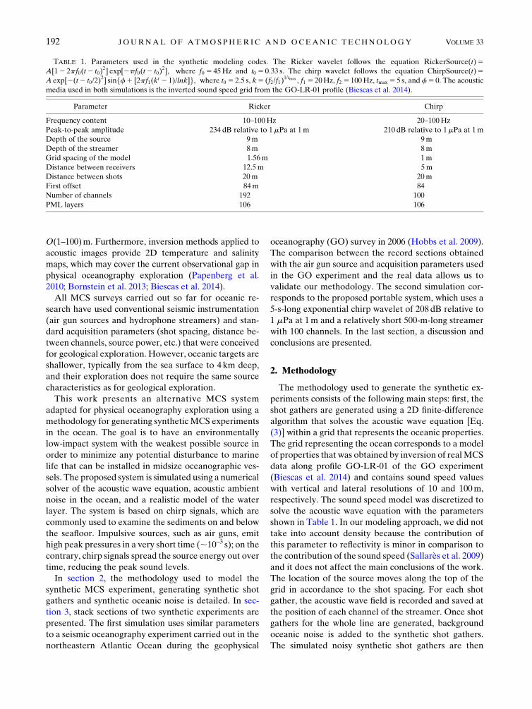
TABLE 1. Parameters used in the synthetic modeling codes. The Ricker wavelet follows the equation RickerSource(t)5A[12 2pf0(t2 t0)

2] exp[2pf0(t2 t0)2], where f0 5 45Hz and t0 5 0:33 s. The chirp wavelet follows the equation ChirpSource(t)5

A exp[2(t2 t0/2)2] sinff1 [2pf1(k

t 2 1)/lnk]g, where t0 5 2:5 s, k5 (f2/f1)1/tmax , f1 5 20Hz, f2 5 100Hz, tmax 5 5 s, and f5 0. The acoustic

media used in both simulations is the inverted sound speed grid from the GO-LR-01 profile (Biescas et al. 2014).

Parameter Ricker Chirp

Frequency content 10–100Hz 20–100Hz

Peak-to-peak amplitude 234 dB relative to 1mPa at 1m 210 dB relative to 1mPa at 1m

Depth of the source 9m 9m

Depth of the streamer 8m 8m

Grid spacing of the model 1.56m 1m

Distance between receivers 12.5m 5m

Distance between shots 20m 20m

First offset 84m 84

Number of channels 192 100

PML layers 106 106

192 JOURNAL OF ATMOSPHER IC AND OCEAN IC TECHNOLOGY VOLUME 33

processed using standard MCS functions to obtain the

stacked section. Finally, the quality of the tested MCS

system is quantified by measuring the spectral signal-to-

noise ratio (SNR) in the stack section.

a. Acoustic source

Two different wavelets are used in the simulations

presented in this work: (i) a Ricker wavelet of 234dB

relative to 1mPa at 1m with a frequency content within

the range of 10–100Hz, which is similar to the wavelet

produced by the source used in the GO-LR-01 profile of

the GO survey and is used to calibrate the synthetic

simulations; and (ii) a 5-s-long exponential chirp wavelet

(Flandin 2001) of 208 dB relative to 1mPa at 1m

amplitude, a Gaussian taper, and a frequency content of

20–100Hz. The Ricker and the chirp wavelets are de-

scribed by the following equations:

RickerSource(t)5A[12 2pf0(t2t

0)2] exp[2pf

0(t2 t

0)2] ,

(1)

where A 5 500 000 is the maximum amplitude of the

wavelet, f0 5 45Hz, and t0 5 0:33 s;

ChirpSource(t)

5A exp

"2

�t2 t

0

2

�2#sin

�f1

�2pf

1

(kt 2 1)

lnk

��,

(2)

where A 5 25 000 is the maximum amplitude of the

wavelet, exp[2(t2 t0)2] with t0 5 2:5 s corresponds to a

5-s-wide Gaussian taper, k5 (f2/f1)1/tmax , tmax 5 5 s, f5 0,

f1 5 20Hz, and f2 5 100Hz. The wavelets, frequency

content, and frequency change in time are shown in

Fig. 1.

b. Synthetic shot gather generation and MCSprocessing

A 2D finite-difference time-domain (FDTD) algo-

rithm with high-order spatial discretization is used to

solve the acoustic wave equation [Eq. (3)] and simulate

the wave propagation through the ocean,

=2p21

c2›2p

t›21 f

s5 0, (3)

where fs is the source function, p is the pressure, and c is

the sound speed. The code includes second-order per-

fectly matched layers (PML) specifically designed for

Seismic Oceanography simulations for the bottom and

side lateral boundaries, while a free-surface condition is

introduced at the top boundary by setting p5 0 at z5 0.

This code was previously presented and validated by

Kormann et al. (2009, 2010). The variables included are

wavelet type, wavelet frequency content, wavelet ampli-

tude, depth and spacing of the acoustic source; number of

channels or receiver groups, distance between them, near

offset and depth of the streamer; recording time; acoustic

media sound speed, grid spacing, and PML layer for ab-

sorbing boundaries. Specific values used in the modeling

are detailed in Table 1. Once the shot gathers are gener-

ated by recording the data at the positions defined by

channel locations along the streamer (Fig. 2a), the syn-

thetic noise is added to each channel and shot (Fig. 2b);

and finally, standardMCSprocessing is applied, consisting

of frequency filter, spherical divergence correction, nor-

mal move-out (NMO) correction with a constant velocity,

and common midpoint (CMP) sort and stack (Fig. 2c).

The chirp simulation has an additional step in which the

data trace from each channel is correlated with the chirp

function (from Fig. 2e to Fig. 2f). The stack from the real

data corresponding to the GO experiment (Fig. 4a) is

obtained by applying the same processing flow. Seismic

UNIX (Cohen and Stockwell 2003) was used for theMCS

processing.

c. Streamer and fold

Since reflection coefficients in oceanic water are

O(1024), the fine structure reflectivity is only weakly de-

tected in a single channel, unless powerful sources are

used (e.g., the source used in the Iberian–AtlanticMargin

Survey, ;240dB relative to 1mPa at 1m; Buffett et al.

2009). However, a key characteristic of MCS systems that

makes them capable of detecting the oceanic fine struc-

ture is the CMP method (Yilmaz 2001), which records

echoes from the same reflection point multiple times from

different angles. The SNR increase is achieved during

data processing, when the recorded signals reflected from

the same subsurface locations and found in the sameCMP

are summed (’’stacked’’ in seismic processing terminol-

ogy). The SNR increases because the amplitudes of the

reflections add coherently, unlike the background noise,

which is random in nature and therefore diminished. The

CMP fold is the number of signals that are summed. It is

proportional to the number of channels in the streamer

and inversely proportional to the shot spacing:

minfold5numchannels3 distance between channels

23 distance between shots

5streamer length

23 distance between shots

(4)

Even though the above-mentioned expression defines

the minimum fold, it can be arbitrary increased by

JANUARY 2016 B I E S CAS ET AL . 193

adding contiguous CMP into the same stacked trace.

The advantage of increasing the fold is that the SNR

increases and the drawback is that the lateral resolution

decreases. The GO-LR-01 data were processed with a

fold of 60 (a 2400-m-long streamer with 192 channels,

12.5-m distance between channels, and 20-m shot spac-

ing), which provided an acceptable SNR of the stacked

data (Fig. 4a). Because one of the interests for the new

MCS system is increasing its portability, a shorter

streamer is proposed in this work, with 100 channels

separated by 5m between them and a 20-m shot spacing.

This geometry results in a nominal CMP spacing (lateral

sampling) of 2.5m. Considering this geometry, Eq. (4)

yields a fold of 12, which would be 5 times smaller than

the one of the GO-LR-01 data and would result in a low

SNR. To achieve an acceptable SNR, we quadruple the

fold to 48 by decreasing the lateral resolution down to

10m by stacking four neighboring CMPs together.

Reducing the spacing between shots would also in-

crease the fold; however, the time length of the chirp

FIG. 1. The 234 dB relative to 1mPa at 1m Ricker wavelet (black) and 5-s exponential chirp of 208 dB relative to

1mPa at 1mwith a Gaussian taper (blue) displayed as (a) time domain, (b) frequency domain, (c) chirp spectrogram,

and (d) Klauder wavelets.

194 JOURNAL OF ATMOSPHER IC AND OCEAN IC TECHNOLOGY VOLUME 33

wavelet limits the minimum distance between shots.

Considering the 5-s chirp and awater layer of 2 km, shots

should be recorded during 7.5 s. Therefore, if the vessel

moves at 4.5-kt speed (2.3m s21), the minimum distance

between shots should be ;17m, which agrees with our

20-m shot spacing.

d. Noise model

To simulate scenarios that are as realistic as possible,

the background noise to be added to the synthetic data is

modeled following these three steps: (i) random ampli-

tudes (absolute maximum amplitude) set independent

for all channels and all shot gathers involved in the

synthetic MCS experiment are generated; (ii) the ran-

dom amplitude signals (white spectra) are convolved

with real recorded noise in the ocean to obtain noise

with realistic spectra; and (iii) spectral levels are set

using the Wenz curves to obtain a medium noise level.

Wenz (1962) gave a detailed analysis of the spectral

characteristics of background oceanic noise from a va-

riety of sources, including the earth’s seismic activity,

ship traffic, wind, waves, bubbles and spray, turbulence,

and rain. The amplitude spectra of the background

oceanic noise generated by the shipping intensity and

the state of the sea, which mainly affect our acoustic

data, were digitized from the results of Wenz (1962) in

order to compare them with the generated synthetic

noise (Fig. 3). This comparison illustrates that the noise

considered in the present work has a frequency content

within the range of realistic noise.

FIG. 2. Shot gather of 192 channels generated (a) with theRickerwavelet of 234 dB relative to 1mPa at 1m, (b) with

synthetic noise, and (c) after applying a frequency filter. Shot gather of 100 channels generated (d) with the 5-s

exponential chirp wavelet of 208 dB relative to 1mPa 1 at 1m, (e) with synthetic noise, and (f) after correlating the

data with the source wavelet and applying a frequency filter.

JANUARY 2016 B I E S CAS ET AL . 195

3. Results

Data computed for the first experiment presented were

produced using parameters (source frequency content

and peak-to-peak amplitude, distances between shots and

receivers, number of channels, first offset and fold) sim-

ilar to those used in theGO-LR-01 profile acquired in the

Gulf of Cadiz (northeast Atlantic Ocean). The acoustic

synthetic source consists of a Ricker wavelet of 234dB

relative to 1mPa at 1m (500000-Pa peak signal), with a

frequency content in the range of 10–100Hz (Fig. 1). To

compare the synthetic and real data, we propagated the

synthetic data through the sound speed model that was

obtained by inverting the MCS data recorded along this

line (Biescas et al. 2014). In particular, the section that we

used is 5km long and images the right edge of a meddy,

which is a typical structure detected in this area that

consists of a warm and salty rotating lens.

A comparison between the real (Fig. 4a) and synthetic

experiments (Fig. 4b) shows remarkable similarity, with

both displaying the same reflectors that correspond to

the oceanic fine structure. The spectra of a part of the

seismic section containing mainly reflected signal (S)

and mostly noise (N) are calculated for both sections

and the corresponding SNR is shown in the upper-right

insets of Figs. 4a and 4b. The SNR of the real data is

slightly lower than the one calculated from the synthetic

experiment (peak at 1.5 vs peak at 2.2), probably due to

additional noise in the real experiment generated by

electronic effects in the hydrophones and the oscilla-

tions of the streamer and source near the sea surface.

Overall, this comparison validates our methodology for

generating realistic synthetic MCS experiments in the

ocean and testing the effect of the involved variables.

The second synthetic experiment (Fig. 4c) simulates

data that would be collected with the portable MCS

system suggested in this work (Table 1) and character-

ized by a significantly lighter and shorter streamer that

could be potentially installed and operated from a

midsize oceanographic vessel. The source wavelet used

in this experiment is a 5-s-long exponential chirp

wavelet of 208 dB relative to 1mPa at 1m (a 25 000-Pa

peak signal) with a Gaussian taper, which minimizes the

sidelobes of the autocorrelation function of the chirp,

and a frequency content of 20–100Hz (Fig. 1).

The stacked section from these synthetic data (Fig. 4c)

shows the meddy fine structure well, and the SNR is

equivalent to that obtained using the impulsive source’s

system. TheRicker source is a signal 20 times stronger in

amplitude than the chirp wavelet. However, as the chirp

wavelet has a 5-s duration, the level of the total energy is

similar to the one emitted by the Ricker pulse, resulting

in similar levels of effectiveness in oceanic exploration.

The low acoustic reflection coefficients in the ocean

(;10–4) create a significant trade-off between de-

tectability and portability of the system. The system

proposed was chosen from several tests that were con-

ducted for this work. However, other combinations of

parameters may give similar SNR by compensating be-

tween the different factors. Figure 5 shows two examples

of unsuccessful systems, with SNR ;1. These two ex-

amples were similar to the one proposed but have (i) a

lower amplitude of the 5-s chirp, 200 dB relative to 1mPa

at 1m; and (ii) a smaller stack fold, 12 instead of 48; and

neither example allows for detection of the meddy fine

structure with a suitable SNR.

4. Discussion and conclusions

MCS systems with air gun sources used for solid Earth

applications have shown to be suitable for deep oceanic

exploration; however, these systems require expensive

instrumentation and vessels. The scientific community

developing ocean seismic visualization is making a joint

effort to find small- and midsize multichannel seismic

systems that could be used to explore the physics of the

ocean (Geli et al. 2009; Carniel et al. 2012; Piété et al.

2013; Ker et al. 2015), but the low reflectivity of the

ocean (R; 1024) makes this goal challenging. In this

work we propose the use of chirp wavelets emitted

with a broadband sound projector source instead of

classical air gun pulses.

We exemplify through numerical simulations that an

oceanic thermohaline structure can be detected with

similar SNR using an impulsive source of 234dB relative

tomPa 1at 1m (a 500000-Pa peak signal) or equivalently a

5-s chirp source of 208dB relative tomPa at 1m (a 25000-Pa

peak signal). The chirp source can reduce the peak of the

pressure signal 20 times by spreading the energy in

FIG. 3. Synthetic noise spectra used in this work (black and solid

curve), shipping noise spectra for seven levels of intensity (Wenz

1962) (gray and spotted curves), and noise related to seven states of

the sea, generated by the wind force (Wenz 1962) (gray and

dashed curves).

196 JOURNAL OF ATMOSPHER IC AND OCEAN IC TECHNOLOGY VOLUME 33

time. There is evidence that a swept signal with lower

peak amplitude may have less impact on marine animals

than a higher peak impulsive signal (Weilgart 2012). For

example, considering the Ricker source, the radius of the

exclusion zone for certain species (an area affected by

more than 160dB relative to 1 mPa) would be 5000m.

That means that, if these species were observed or de-

tected with passive acoustic monitoring, closer than

FIG. 4. (a) Stack section of 5 km long of the GO-LR-01 profile acquired in the GO survey

(Gulf of Cadiz, northeast Atlantic Ocean, April–May 2006). (b) Stack section of the synthetic

data generated with the 234 dB relative to 1mPa at 1m Ricker wavelet. (c) Stack section of the

synthetic data generated with the 208 dB relative to 1mPa 1 at 1m 5-s exponential chirp

wavelet. The upper-right white insets correspond to the SNR of the data within the two cor-

responding rectangles.

JANUARY 2016 B I E S CAS ET AL . 197

5000m to the air guns, these air guns had to be immedi-

ately shut down. Since the energy of the source decreases

with the square of the distance, and since the energy is

proportional to the square of the amplitude of the emitted

signal, then the exclusion zone for the proposed system

would be A2R/d

2R 5A2

Ch/d2Ch, dCh 5

ffiffiffiffiffiffiffiffiffiffiffiffiffiffiffiffiffiffiffiffiffiA2

Chd2R/A

2R

q5 250m;

thus, the mitigation distance for these species would be

20 times shorter than with the impulsive signal.

Regarding the frequency content of the source, it is

known that the vertical resolution of acoustic data in-

creases proportionally with the frequency content of the

source. Consequently, a high-frequency seismic source

would provide better vertical resolution. In spite of that,

high-frequency sources (f . 200Hz) tested in previous

seismic oceanography (SO) surveys provided low SNR

and a fine structure that was poorly detected with these

sources (Geli et al. 2009; Ker et al. 2015), even though

the background noise decreases when increasing fre-

quencies (Fig. 3). To test frequencies higher than

100Hz, we modeled two chirp wavelets through a syn-

thetic medium obtained by expanding a single CTD

profile to a horizontally uniform 2D sound speed model.

Thisway,weproduced a sound speedmodelwith a vertical

resolution of 1m, which allowed us to test sources with a

frequency content up to 375Hz. Chirp wavelets were 5 s,

208dB relative to 1mPa at 1m peak amplitude, and had a

frequency content of 10–150 and 150–300Hz (Fig. 6). The

same level of synthetic background noise was added to the

shots, and the comparison between both stack sections

shows clearly that SNR decreases progressively as fre-

quency increases (Fig. 6). Since the seismic signal is

FIG. 5. Stack sections of the synthetic data generatedwith (a) 200 dB relative to 1mPa at 1m5-s

exponential chirpwavelet andprocessedwitha foldequal to60and(b)208dBrelative to1mPaat1m5-s

exponential chirp wavelet and processed with a fold equal to 15. The upper-right white insets

correspond to the SNR of the data within the two corresponding rectangles.

198 JOURNAL OF ATMOSPHER IC AND OCEAN IC TECHNOLOGY VOLUME 33

the result of the convolution between the source wavelet

and the reflectivity of the media, we have calculated the

spectra of the reflectivity data from a CTD (upper-right

inset in Fig. 6a) and it shows that oceanic reflectivity

amplitude decreases with frequency, which supports the

low SNR with high-frequency sources. The work pre-

sented by Ker et al. (2015) analyzes ocean reflectivity in

terms of the frequency emitted from the source and the

thickness of the thermocline to be detected, and cor-

roborates that the signal amplitude decreases with in-

creasing frequency regardless of the thermocline’s

thickness. Nevertheless, the optimal frequency content

remains an open question and will strongly depend

on the fine structure to be detected in each single

experiment.

Problems regarding phase dispersion caused by the

Doppler effect have been described in the use of

marine vibrators (Dragoset 1988). We may note that

even though dips in oceanic reflectors are generally

very smooth, this effect would increase by increasing

the frequency bandwidth and duration of the sweep,

which should be taken into account in the design of

the pulse.

The system that we propose in this work compensates

for a shorter streamer and relatively low chirp source

amplitude with a longer time duration. It would provide

thermohaline information of the full-depth water

column and along lateral distances of hundreds of kilo-

meters in the ocean, with lateral and vertical resolutions

on the order ofO(10)m. This proposed system could be

the starting point for the development of an ocean-specific

low-frequency acoustic projection system for physical

oceanography.

Acknowledgments. The first author’s work has been

supported by the European Commission through Marie

Curie Actions FP7-PEOPLE-2010-IOF-271936 and

FP7-PEOPLE-2012-COFUND-600407. This work has

been done in the framework of the Spanish project

POSEIDON (CTM2010-25169) and the ItalianNational

FlagshipProgrammeRITMARE (ProgrammaNazionale

della Ricerca 2011-2013 MIUR). We want to acknowl-

edge the team of GO project funded by the EU (015603-

GO-STREP).

REFERENCES

Biescas, B., V. Sallarès, J. Pelegrí, F. Machín, R. Carbonell,

G. Buffett, J. Dañobeitia, and A. Calahorrano, 2008: Imaging

meddy finestructure using multichannel seismic reflec-

tion data. Geophys. Res. Lett., 35, L11609, doi:10.1029/

2008GL033971.

——, L. Armi, V. Sallarès, and E. Gràcia, 2010: Seismic imaging

of staircase layers below the Mediterranean undercur-

rent. Deep-Sea Res. I, 57, 1345–1353, doi:10.1016/

j.dsr.2010.07.001.

——, B. Ruddick, M. Nedimovi�c, V. Sallarès, G. Bornstein, and

J. Mojica, 2014: Recovery of temperature, salinity, and po-

tential density from ocean reflectivity. J. Geophys. Res.

Oceans, 119, 3171–3184, doi:10.1002/2013JC009662.

Bornstein, G., B. Biescas, A. Sallares, V. Bower, and J. Mojica,

2013: Direct temperature and salinity acoustic full waveform

inversion. Geophys. Res. Lett., 40, 4344–4348, doi:10.1002/

grl.50844.

Buffett, G., B. Biescas, J. Pelegrí, F. Machín, V. Sallarès,R. Carbonell, D. Klaeschen, and R. Hobbs, 2009: Seismic

reflection along the path of the Mediterranean Un-

dercurrent. Cont. Shelf Res., 29, 1848–1860, doi:10.1016/

j.csr.2009.05.017.

Carniel, S., A. Bergamasco, J. Book, R. W. Hobbs, M. Sclavo, and

W. Wood, 2012: Tracking bottom waters in the Southern

FIG. 6. (a) CTD sound speed profile used for themodel and spectra of the reflectivity from the CTDdata (upper-right inset). Stack sections

obtained with the 5-s chirp, 205 dB relative to 1mPa 1 at 1m, and frequency content of (b) 10–150 and (c) 150–300Hz.

JANUARY 2016 B I E S CAS ET AL . 199

Adriatic Sea applying seismic oceanography techniques.Cont.

Shelf Res., 44, 30–38, doi:10.1016/j.csr.2011.09.004.

Cohen, J., and J. Stockwell, 2003: CWP/SU: Seismic Unix release

No. 36: A free package for seismic research and processing.

Center for Wave Phenomena, Colorado School of Mines, 153

pp.

Dragoset, W., 1988: Marine vibrators and the Doppler effect.

Geophysics, 53, 1388–1398, doi:10.1190/1.1442418.Flandin, P., 2001: The frequency and chirps. Wavelet Applications

VIII, H. H. Szu et al., Eds., International Society for Optical

Engineering (SPIE Proceedings, Vol. 4391), 161–175,

doi:10.1117/12.421196.

Geli, L., E. Cosquer, R. Hobbs, D. Klaeschen, C. Papenberg,

Y. Thomas, C. Menesguen, and B. Hua, 2009: High resolution

seismic imaging of the ocean structure using a small volume

airgun source array in the Gulf of Cadiz. Geophys. Res. Lett.,

36, L00D09, doi:10.1029/2009GL040820.

Hobbs, R., D. Klaeschen, V. Sallarès, K. Vsemirnova, and

C. Papenberg, 2009: Effect of seismic source bandwidth on

reflection sections to image water structure. Geophys. Res.

Lett., 36, L00D08, doi:10.1029/2009GL040215.

Holbrook, W., I. Fer, R. Schmitt, D. Lizarralde, J. Klymak,

L. Helfrich, and R. Kubiche, 2013: Estimating oceanic turbu-

lence dissipation from seismic images. J. Atmos. Oceanic

Technol., 30, 1767–1788, doi:10.1175/JTECH-D-12-00140.1.

Hua, B., C. Ménesguen, S. Le Gentil, R. Schopp, B. Marsset, and

H. Aiki, 2013: Layering and turbulence surrounding an anti-

cyclonic oceanic vortex: In situ observations and quasi-

geostrophic numerical simulations. J. Fluid Mech., 731, 418–

442, doi:10.1017/jfm.2013.369.

Ker, S., Y. Le Gonidec, L. Marié, Y. Thomas, and D. Gibert, 2015:

Multiscale seismic reflectivity of shallow thermoclines. J.Geophys.

Res. Oceans, 120, 1872–1886, doi:10.1002/2014JC010478.

Kormann, J., P. Cobo, M. Recuero, B. Biescas, and V. Sallarès,2009: Modelling seismic oceanography experiments by using

first- and second-order complex frequency shifted perfectly

matched layers. Acta Acust. Acust., 95, 1104–1111,

doi:10.3813/AAA.918242.

——,——, B. Biescas, V. Sallarès, C. Papenberg, M. Recuero, and

R. Carbonell, 2010: Synthetic modelling of acoustical propa-

gation applied to seismic oceanography. Geophys. Res. Lett.,

37, L00D90, doi:10.1029/2009GL041763.

Ménesguen, C., B. Hua, C. Papenberg, D. Klaeschen, L. Géli, andR. Hobbs, 2009: Effect of bandwidth on seismic imaging of

rotating stratified turbulence surrounding an anticyclonic

eddy from field data and numerical simulations.Geophys. Res.

Lett., 36, L00D05, doi:10.1029/2009GL039951.

Papenberg, C., D. Klaeschen, G. Krahmann, and R. Hobbs, 2010:

Ocean temperature and salinity inverted from combined hy-

drographic and seismic data. Geophys. Res. Lett., 37, L04601,

doi:10.1029/2010GL042115.

Piété, H., L. Marié, B. Marsset, Y. Thomas, and M.-A. Gutscher,

2013: Seismic reflection imaging of shallow oceanographic

structures. J. Geophys. Res. Oceans, 118, 2329–2344,

doi:10.1002/jgrc.20156.

Pinheiro, L., H. Song, B. Ruddick, J. Dubert, I. Ambar, K.Mustafa,

and R. Bezerra, 2010: Detailed 2-D imaging of the Mediter-

ranean outflow and meddies off W Iberia from multichannel

seismic data. J. Mar. Syst., 79, 89–100, doi:10.1016/

j.jmarsys.2009.07.004.

Quentel, E., X. Carton, M.-A. Gutscher, and R. Hobbs, 2010:

Detecting and characterizing mesoscale and submesoscale

structures of Mediterranean water from joint seismic and hy-

drographic measurements in the Gulf of Cadiz.Geophys. Res.

Lett., 37, L06604, doi:10.1029/2010GL042766.

Ruddick, B., 2003: Sounding out ocean fine structure. Science, 301,

772–777, doi:10.1126/science.1086924.

Sallarès, V., B. Biescas, G. Buffett, R. Carbonell, J. Dañobeitia,and J. Pelegrí, 2009: Relative contribution of temperature and

salinity to ocean acoustic reflectivity. Geophys. Res. Lett., 36,

L00D06, doi:10.1029/2009GL040187.

Smith, K., and R. Ferrari, 2009: The production and dissipation

of compensated thermohaline variance by mesoscale

stirring. J. Phys. Oceanogr., 39, 2477–2501, doi:10.1175/

2009JPO4103.1.

Vsemirnova, K., R. Hobbs, and P. Hosegood, 2012: Mapping tur-

bidity layers using seismic oceanography methods.Ocean Sci.,

8, 11–18, doi:10.5194/os-8-11-2012.

Weilgart, L., 2012: Are there technological alternatives to air guns

for oil and gas exploration to reduce potential noise impacts

on cetaceus? The Effects of Noise on Aquatic Life, A. Popper

and A. Hawkins, Eds., Advances in Experimental Medicine

and Biology, Vol. 730, Springer New York, 605–607,

doi:10.1007/978-1-4419-7311-5_137.

Wenz, G., 1962: Acoustic ambient noise in the ocean: Spectra and

sources. J. Acoust. Soc. Amer., 34, 1963–1956, doi:10.1121/1.1909155.

Yilmaz, O., 2001: Seismic Data Analysis: Processing, Inversion, and

Interpretation of Seismic Data. 2nd ed. Society of Exploration

Geophysicists, 2027 pp.

200 JOURNAL OF ATMOSPHER IC AND OCEAN IC TECHNOLOGY VOLUME 33