RCEP/WP no.4/October 2000

SUSTAINABILITY OF THE PUBLICDEBT AND BUDGET DEFICIT

DR. LUCIAN-LIVIU ALBUInstitute for Economic Forecasting, Romanian Academy of Sciences

DR. ELENA PELINESCUNational Bank of Romania and Institute for Economic Forecasting

1

– Abstract –

This study is designed primarily for the project “Romania – Country EconomicMemorandum” and “Romania 2000” conference that will be organised by the World Bankand Romanian Center for Economic Policies in October. It should also be helpful togovernment officials responsible for managing the external debt of Romania and to thosewith a general interest in public sector financial management in an economic system intransition --observers as well as practitioners.

This study attempts to explain the evolution of the external debt and budget deficitduring the 1990-1998 period and attributes it to the general economic environment andmacroeconomic policies applied in each sub-period. In doing so, the interrelationshipbetween the progress in reforming the fiscal system and sustainability of budget deficits isanalysed, as is the importance of fiscal income in partly determining public debt. A largerange of the impacts of external debt and budget deficit management is discussed, includingthe ramifications for the money supply, inflation rate, interest rate, exchange rate, seigniorageand inflation tax, the contributions of privatisation and the re-allocation of resources, etc.

Special attention is dedicated to the breakpoint represented by the year 1997 when thebudget deficit management and fiscal system were fundamentally changed. There are someestimations and useful ideas for macroeconomic policy makers presented for the post-2000period, obtained by using a simulation-sustainability model.

1

1. Introduction

At the beginning of the transition period in 1990, the public debt in Romania wasinsignificant. During the following years, the accumulation process accelerated. By 1998, thedomestic public debt, together with the country’s external debt, already increased to nearly40% of Gross Domestic Product. Although the indebtedness degree of the country continuesto be smaller than levels registered in other European countries, more dangerous is itsaccelerating trend in conditions of some not so very high-performing macroeconomic policymanagement. In order to adhere to NATO and European Union actions and agreements withinternational financing institutions, such as the International Monetary Fund and the WorldBank, the problem of public debt and budgetary deficits has become more and more sharp.The major difficulties proceed from weak performance of the Romanian economy doubled bythe complex problems of economic reform and restructuring, but also by more restrictedaccess to external financing on international markets.

The present paper attempts to answer certain questions related to governancemechanisms of public debt accumulation. In particular, it examines: a) some of the mostimportant implications of public sector deficits on the dynamics of main macroeconomicindicators; b) factors that impact the degree of sustainability; and c) the possibilities forsetting up fundamental parameters and a time horizon to stop the debt accumulation process.Certain plausible hypotheses will be selected and a few likely evolutions will be simulated.

2. The dynamics of public debt after 1989

There are various approaches in specialised literature regarding public debt and thepublic sector. In most official publications referring to public debt, the public sector is the“general government” or consolidated non-financial public sector, which consists of thecentral government, the local authorities and non-private social security and otherorganisations (this is the definition also used within our paper). Others add certain publiccorporations, while in many cases, some special credit institutions are also included in thedefinition. Similarly, certain publications refer to gross debt, others to net debt (i.e. gross debtnet of public sector liquid assets); while in some cases more assets are netted out.

The exclusion of state financial institutions from the conventional definition of thepublic sector creates some problems. This is particularly the case in Romania where the Stateis the majority shareholder of most of the domestic commercial banks and two special creditinstitutions belong entirely to it. Almost all the domestic liabilities of public corporations andmost of the domestic liabilities of the central government itself are assets of banks and creditinstitutions, partially or wholly owned by the State. This implies: a) that the size of thepublic debt may be very sensitive to the definition of the public sector, and b) thatseigniorage revenue, which is defined as the change in the monetary base in real terms, may

2

accrue to the public sector, as it is conventionally defined here, in an indirect and not easilydetectable way.

A particular criticism of the conventional definitions of public debts and deficits is theasymmetry in the treatment between the private and the public sectors in the presentation oftheir accounts. It is argued that instead of public debt, the concept of public net worth shouldbe used, while the annual public deficits should be split between consumption and investmentdeficits (Eisner, 1989; Stournaras, 1990). Although this criticism is correct, the data neededto evaluate public sector assets makes it an impossible task. However, the ratio betweenconsumption and investment deficits has serious implications for the sustainability of anincreasing public debt, the transfer of burden on future generations and the balance ofresources in the economy. It also provides a proxy for the evolution of the public sector’s networth (Odling-Smee and Riley, 1985). Therefore, it should be a necessary component in anystudy of public debts and deficits.

During the period after 1989, Romania faced more public debt accumulation as a newmatter of macroeconomic policy, in contrast to other Central and East European countriessuch as Bulgaria, the Czech Republic, Hungary, or Poland. While the external debt ofRomania was insignificant in 1990 (US$230 million), the other Central and East Europeancountries were already confronted with debt amounts of many billions of US dollars(Hungary – US$21.3 billion, Bulgaria – US$10.9 billion, Czech Republic – US$4.4 billion).In the case of Poland, the figure was close to US$50 billion. Eight years later, in 1998, theexternal debt of Romania already increased to more than 9 billion USD, while the othercountries (with the exception of the Czech Republic, where external debt was five timeslarger than in 1990) registered either a modest growth (e.g. the case of Hungary with growthof US$5.5 billion) or even a diminution (Poland with more than US$6 billion, partiallycaused by cancellation of a proportion of its external debt, and in Bulgaria with US$1billion). One of the weakest performances of the Romanian economy after 1989 was the poorexperience regarding the management of public debt and budget deficits.

The evolution of external debt in Romania, as a share of GDP evaluated in US dollarsand respectively in Lei, is shown in Figures 1 and 2. The statistical data on which the graphswere based is presented in Appendix 1.

In Romania, contrary to advanced countries, the external debt is the main componentof total debt. However, in later years one can see that the accumulation of domestic publicdebt became a more important source to cover deficits. For instance, in 1998 it representedclose to 8% of GDP. This evolution is in direct connection with efforts to improve themanagement of domestic debt, especially by enacting a new rule in April 1997 regarding thedevelopment of a secondary market for state obligations, restricting access to external sourcesof financing, and taking over in public debt an important volume of non-efficient credits. Forinstance, the share of state loans approved by special normative documents evolved asfollows: in 1992 – 8.1%; in the 1993-1996 period– an average level of 5.7% (with amaximum share of 11.7% in 1995); and in 1998-1999 – more than 30% during anaccelerating restructuring process of the banking system.

It is remarkable to see that Romania has also begun to demonstrate the correlationbetween election cycles and accumulation of public debt. We can observe the jumps in

3

electoral years on the presented graphs--1992 and 1996--followed by calm debt accumulationdynamics between the two election moments. In the literature, there is a serious focus onevaluating the impact of political environment dynamics on public debt accumulation. Someauthors even sought to quantify this impact (Roubini and Sachs, 1989). One of the mostimportant conclusions of such studies is that there is a direct correlation between the degreeof homogeneity of power coalitions and the dynamics of public sector deficits. As a verifiedrule, when the leading political coalition has a large number of parties with various politicalorientations, as is the actual situation in Romania, then the budget policy loses its coherenceand deficits will increase. On the contrary, in countries where the political power is in thehands of only one strong party, the chance to apply an efficient management of public debt isgreater.

The evolution of the gap between the share of debt in GDP evaluated in dollars andthat expressed in Lei, shown on the graph in Figure 3, reflects the impact of domesticcurrency depreciation (the value of external debt being converted by the Lei/USD exchangerate at the end of each year). Moreover, the evolution in the 1990-1998 period in Romaniademonstrates a strong reverse correlation between the change of the rate of real GDP and thedynamics of the mentioned gap (see Figure 4).

Figure 1 Figure 2

Figure3 Figure 4

1990 1992 1994 1996 19980

0.1

0.2

0.3

0.4

dtb_d%t

dExb_d%t

dInb_d% t

t1990 1992 1994 1996 1998

0

0.1

0.2

0.3

0.4

dtb_L%t

dExb_L%t

dInb_L%t

t

1990 1992 1994 1996 19980

0.1

0.2

0.3

0.4

dtb_L%t

dtb_d%t

t1990 1991 1992 1993 1994 1995 1996 1997 1998

15

10

5

0

5

10

15

∆ dtbt

r%t

t

4

Figure 5 Figure 6

Another important aspect of analyses regarding the evolution of the public debt isrepresented by the distinction among main institutional sectors. In Romania, as we alreadymentioned, besides the conventional public debt owned by the so-called general governmentthere is a part which corresponds to public corporations and special credit institutions.Figures 5 and 6 present the evolution of the three constitutive components of gross publicdebt, evaluated in dollars and respectively in Lei, computed with the exchange rate baseregistered at the end of each year.

The first line at the bottom of the graphs represents the dynamics of governmentaldebt, the second line traces the evolution of the gross public debt, and the third one, at the topof the graphs, expresses the evolution of the country’s gross debt. The difference betweenthe middle and first curve could be interpreted as gross public corporation debt, but the gapbetween the curve placed on the top and middle of the graphs represents the share of the non-public sector. Moreover, during the considered period, we can see an amplification trend ofthe two gaps which indicates a decrease in the share of government debt--both in gross publicsector debt and in gross country debt.

Despite Romania's classification by the World Bank in international statistics as a“ less indebted” country, together with Poland, Croatia, the Slovak Republic, Czech Republic,Estonia, etc. (while Hungary is classified as “moderately indebted” and Bulgaria as “severelyindebted”), some alarming signals were emitted by certain external financing institutions lastyear. With a background of continuing economic recession for the consecutive third year anda rapid external debt-service burden, certain international agencies specialised in evaluatingcountry risk declassified Romania’s score. One of the most important arguments was theworsening of sustainability indicators in correlation with other negative occurrences, such asdiminishing accumulation resources, decreasing domestic savings and investment rates, andincreasing risk for foreign investments [1]. The fact that more than 90% of the grosscountry’s debt is externally financed demonstrates the fragility of the national economy andthe high degree to which it depends on external financing conditions for collecting newresources. In such conditions, the sustainability problem, already intensely preoccupyingexternal financing institutions of Romania, should have to give serious incentives to thosehaving an impact on macroeconomic policy decisions, especially to government.

1990 1992 1994 1996 19980

0.1

0.2

0.3

0.4

dtb_d%t

dtpb_d% t

dtgb_d% t

t

1990 1992 1994 1996 19980

0.1

0.2

0.3

0.4

dtb_L%t

dtpb_L%t

dtgb_L%t

t

5

3. An Estimation of the parameters in an equation of public debt dynamics

Quantifying the dynamics of public sector debt often starts from the well-knowndefinition of the government’s budget constraint. The change in the public sector debt Dbetween two time periods, t and t –1, is given by the following equality:

D t – D t – 1 = i t D t – 1 + Π t + a t D t – 1 – ∆B t (1)

where i is the average nominal interest rate on public sector debt, Π is the primary deficit(PSBR net of interest payments), a is the revaluation effect on existing debt (in Romania thisis entirely due to the depreciation of the effective exchange rate of the Leu, since public debtis not sold, at least up to now, below or above its redemption value) and ∆B is the directfinancing of the budget from the Central Bank [2].

Certain methodological remarks are due here. According to the Treasury’s definition,the central government debt includes, among other liabilities, long-term loans made availableto the government by the National Bank of Romania as well as treasury bills sold to the NBR.These long-term loans and treasury bills create debt service obligations for the centralgovernment. The implication is that ∆B in equation (1) is not the change in the monetarybase, ∆M, but part of it, determined by changes in a special government account with theBank. Another related point is the allocation of seigniorage revenue. Although the NBRdoes not pay dividends to the Treasury, it subsidises the activities of various commercialbanks and special credit institutions partly or wholly owned by the State whose assets andliabilities are not included in the definition of public debt.

The direct financing of the budget from the NBR is the change, ∆B, in the outstandingbalance of the government account with the Bank. When these accounts show a negativebalance, this cannot exceed a certain limit set by law. It is this (constrained) change in thebalance of this account that constitutes direct financing of the PSBR by the NBR and is notconsidered by the Treasury as additional debt. It should be noted that the effective limitconstraining direct financing is lower than the one set by the law, because a (small) interestrate is charged on negative balances.

Finally, due to non-accurate primary statistical data, we used D, the public-sectorgross debt (excluding government guaranteed debt) in order to evaluate the dynamics ofpublic sector debt, and obtained ∆B as the difference between the sum of the first threecomponents of equation (1) and ∆D. Then, dividing both sides of equation (1) by thenominal GDP, Yt , and manipulating we obtain:

d t – d t – 1 = ( i t + a t – g t ) [ d t – 1 / ( 1 + g t ) ] + π t – b t (2)

where dt and dt–1 are the public sector debt to GDP ratio in two consecutive years, tand t –1, π is the primary public sector deficit as a percentage of GDP, g is the nominal GDPgrowth rate between years t and t -1 and b is ∆B/Y. Alternatively, we can approximate thenominal growth rate g as the sum of the change in GDP deflator p and the real GDP growthrate q and rewrite equation (2) as:

6

d t – d t – 1 = ( i* t – q t) [ d t – 1 / ( 1 + g t ) ] + π t – b t (3)

where i* is defined as the real effective average interest rate on public sector debt--itis equal to the average real interest rate, i – p, plus the revaluation effect, a. Because ofspecific situations in Romania during this period, we considered the following two cases: 1) –including general government proceeds from privatisation and 2) – excluding them.Privatisation income contributed to the amelioration of the government budget for the actualperiod and probably for the next few years. However, viewing the dynamic equation of publicdebt in the long run, it would be excluded.

Applying equation (3) to explain the evolution of central government debt relative toGDP for which data on interest payments is more reliable in comparison to that regardinggeneral government or total public sector debt, we obtain Table 1.

Table 1. The Evolution of the Central Government Debt to GDP Ratio(Percentage Points)

d t – d t – 1 π t (i* t – g* t) d t – 1

1 + g t

b t Discrepancy(2)+(3)-(4)-(1)

i – p a t i* t q t ∆Μ tY t

(1) (2) (3) (4) (5) (6) (7) (8) (9) (10)

1990 0.7 -1.0 0.5 -1.2 0.00 -13.6 301.3 287.7 -5.6 …1991 7.9 -3.3 6.6 -4.5 -0.09 -186.1 2047 1861 -12.9 …1992 10.2 4.4 5.5 0.3 -0.57 -184.4 347.6 163.1 -8.8 …1993 1)

2)-1.8-1.4

-0.6-0.2

-0.9-0.7

0.10.3

+0.19+0.19

-207.4 192.4196.9

-15.0-10.5

1.5 3.4

1994 1)2)

-4.1-3.8

0.51.2

-4.5-4.6

-0.30.1

+0.38+0.38

-114.4 52.753.9

-61.7-60.4

3.9 3.9

1995 1)2)

1.92.4

1.22.4

2.52.7

1.62.5

+0.23+0.24

-17.5 52.153.6

34.636.1

7.1 2.0

1996 1)2)

6.16.5

2.23.8

4.75.1

0.62.1

+0.18+0.19

-25.3 76.676.5

51.351.2

3.9 2.9

1997 1)2)

0.4-0.2

0.11.1

1.51.3

2.13.6

-0.93-1.00

-107.2 116.5113.2

9.36.0

-6.9 1.1

1998 1)2)

2.13.4

-2.10.2

4.75.2

1.02.6

-0.54-0.56

-17.5 39.641.6

22.124.1

-7.3 2.5

Total 1)1989-98 2)

23.325.7

1.48.5

20.521.7

-0.35.8

-1.1-1.2

Average 1)1990-98 2)

2.62.9

0.20.9

2.32.4

0.00.6

-0.1-0.1

-97.0-97.0

358.4359.1

261.4262.0

-2.8-2.8

2.6 3)

Average 1)1990-92 2)

6.36.3

0.00.0

4.24.2

-1.8-1.8

-0.2-0.2

-128.0-128.0

898.7898.7

770.7770.7

-9.1-9.1

…

Average 1)1993-96 2)

0.50.9

0.81.8

0.40.6

0.51.3

0.20.3

-91.1-91.1

93.495.2

2.34.1

4.14.1

3.1

Average 1)1997-98 2)

1.21.6

-1.00.7

3.13.2

1.63.1

-0.7-0.8

-62.4-62.4

78.177.4

15.715.0

-7.1-7.1

1.8

1) including general government proceeds from privatisation2) excluding general government proceeds from privatisation3) 1993-98

7

The following conclusions can be drawn:

a) equation (3) predicts an acceptable evolution of the central government debt toGDP ratio for the whole period 1989-1998 (see the sum of discrepancies and their average incolumn 5), but much better for the sub-periods, although the year to year discrepanciesappear to be significant for a number of years. This is mainly due to changing accountingpractices regarding the treatment of capitalised interest payments on central government debtsold to NBR and the use of the trade weighted – rather than debt weighted – effectiveexchange rate to estimate the revaluation effects owing to the depreciation of the Leu;

b) the main cause of the increase in the debt to GDP ratio is the aggregate representedby column 5, which includes the impact of the real effective average interest rate on publicsector debt (i* ) in correlation with the real GDP growth rate (q) and inflation rate, by agencyof the nominal GDP growth rate (g). For a number of years, the main cause is the primarydeficit to GDP ratios;

c) exclusion of income from privatisation would produce a major impact both on theprimary deficit side (π) and on direct financing from the Central Bank (b). This must be animportant signal for authorities to the moment when the privatisation process will be finished;

d) after 1994, the dimension of parameter b became comparable with the averagechange in the monetary base relative to GDP (column 10).

4. Impact of the fiscal position on debt sustainability

Another important determinant of the debt dynamics that appears in equation (1) isthe primary fiscal balance. A permanent increase in the fiscal primary surplus would improvedebt sustainability through: (i) reducing the real interest rate by crowding out reduction; (ii)increasing income by increasing efficiencies in resource allocation and reduced interest rates;(iii) and increasing the demand for the money base as a result of reduced inflationaryexpectations (Garcia, 1998). Generally, large primary deficits are the story behind theaccumulation of public debts and are in direct correlation with the development ofconventional deficits.

Analysis of both the financial position and public debt composition during 1990-99 isthe first step towards finding an answer to the question of whether fiscal policy can strike abalance by fending off debt accumulation and the extent to which the current debt can becurtailed through the achievement of a surplus in the future. Conventional deficits of thecentral government were kept under control between 1990-98; Romania’s performance in thisarea is better than that of Hungary or Bulgaria, but worse than that of the Czech Republic,Croatia, Slovakia or Poland (as set out in the table of Appendix 2).

Moreover, conventional deficits of the non-financial consolidated public sector postedlarge swings on an annual basis—ranging from 0.4% to 4.6% of GDP—which may beregarded as moderate. Behind these developments stood the reform of the fiscal system that

8

was aimed at alleviating imbalances. Its influence on the volume and composition ofincomes and expenditures is highlighted by data in Table 2 (the yearly data is also presentedin Appendix 3).

Figures show that even once primary adjustment has taken place, the imbalance cantake on a life of its own due to large outstanding debts and high interest payments. Inaddition, an average decrease in tax revenue by 4.8 percentage points from 1990-1991 to1997-1999 led to higher expenditures because the government tried to cover generous socialsupport programmes that replace high proportions of lost earnings. The exclusion of moreand more people from the labour force generated by the restructuring process—theunemployment rate increased to 11.3% in July 1999—means that fewer workers aresupporting a growing number of unemployed and retirees through higher tax burdens. In1998, the social security deficit balance increased to 0.9% of GDP. Because the change in taxrevenue and government expenditures had different effects on debt sustainability, thecomposition of fiscal adjustment is a critical variable.

Table 2. Change in the Consolidated General Government Balance

Average Average Change Average Change Average1990-1991 1992-1996 1997-1999 1990-1998

TOTAL REVENUE 40.8 33.1 -7.8 36.0 2.9 34.7 Current 39.2 32.8 -6.4 33.8 1.0 33.8 A. Tax 34.3 29.7 -4.6 31.8 2.1 30.6 A1. Direct tax 23.2 20.9 -2.3 19.6 -1.3 20.6 Profit tax 6.1 4.0 -2.0 3.8 -0.2 4.4 Tax on salaries 7.2 6.6 -0.5 6.0 -0.7 6.5 Social security 8.9 8.6 -0.3 8.8 0.2 8.5 contributions Other 1.0 1.6 0.6 1.0 -0.6 1.2 A2. Indirect tax 11.2 8.9 -2.3 12.3 3.4 10.0 out of which: Excises and oil tax 10.0 3.0 -7.0 2.5 -0.5 4.4 V.A.T. 0.0 3.7 3.7 6.2 2.5 3.3 Customs tax 0.6 1.4 0.7 1.6 0.3 1.2 Other 0.5 0.9 0.4 1.9 1.1 1.1 B. Nontax 4.8 3.1 -1.8 2.0 -1.1 3.3 Capital 1.6 0.3 -1.4 2.1 1.8 0.9 Others 0.0 0.0 0.0 0.1 0.1 0.0TOTAL EXPENDITURES 38.7 35.7 -3.0 39.5 3.8 36.5 Current 31.8 30.2 -1.5 35.3 5.1 30.9 Goods and services 12.9 12.6 -0.4 13.3 0.7 12.5o/w: Wages and salaries 7.4 6.7 -0.7 5.8 -0.9 6.5 Interest payments for public debt 0.0 1.1 1.1 5.0 3.9 1.6 Subsidies and transfers 20.7 18.8 -1.9 16.8 -2.0 18.4 Subsidies 10.0 8.7 -1.3 2.4 -6.3 7.5 Transfers 10.7 10.1 -0.6 14.4 4.3 10.9 Capital 6.9 4.9 -2.1 3.7 -1.2 5.2 Lending minus repayments 0.0 0.5 0.5 0.5 0.0 0.4 OVERALL BALANCE (cash-net of 2.1 -3.4 -5.6 -5.5 -2.1 -2.6 privatisation receiptsOVERALL BALANCE (cash- 2.1 -2.7 -4.8 -3.5 -0.9 -1.8including privatisation receipts) PRIMARY Balance (including private) 2.2 -1.5 -3.7 1.6 3.1 -0.2 PRIMARY Balance (excluding private) 2.2 -2.3 -4.5 -0.4 2.0 -0.9

9

During the transition period, the composition of income was affected by numerousmeasures. The previous confiscated profit transfer tax was abolished in 1990 and replacedwith a profit tax and was reformed in 1991 and again in August 1994 (currently, the rate is38%). The inefficient turnover tax gave way to the VAT in July 1993. There was an initial,single 18% rate, followed by the introduction of a minimum level of 9% in 1994 for certainfood items and medicines. The VAT was readjusted in February 1998 by increasing the taxrates for the above items from 9 to 11%, and from 18 to 22%, respectively. The former wagetax, based on the economy-wide gross average wage, was replaced with an individual wagetax which broadened the tax base by substantially reducing the number of exemptions. Inaddition, the enforcement of some regulations on the luncheon vouchers was delayed in 1999and tax incentives were provided to strategic investors. Tax reforms introduced in 1998envisaged an 8.1 percent increase in indirect taxes in H1 1999 compared to 1998 with asimultaneous reduction of direct taxes. The top priority for the year 2000 will be to enforcethe personal income tax that encompasses all sources of personal income.

In the first years of transition, a few major decisions were taken to formulate a publicexpenditure strategy. They included the increased routing of expenditures through newlyestablished extra-budgetary funds and accounts, improved transparency and accountability,and the establishment of the Treasury Directorate and Public-Debt Directorate. Control overexpenditures in 1993 through 1995 was also reformed, except for spending on wages,salaries, pensions, benefits, and welfare payments. Subsidies and transfers were sharply cutand transparently incorporated into the government budget.

Therefore, during 1990-98, revenues and expenditures as a percentage of GDPfluctuated within a margin of as much as 32 to 42%. The composition of expenditures showsthe swift pace of self-sustaining public debt through ever-increasing costs incurred by publicdebt service, reaching a 6.25% share-to-GDP ratio in the first half of 1999 from 0.2% in1992. Transparent subsidies granted from the government budget to state-owned enterprisesundergoing restructuring, along with the abolition of the window for financing the quasi-fiscal deficit through directed credits and interest-rate subsidies in 1992 to 1996, enabledpolicymakers to assess the real size of the economic imbalances and to implement severalcorrective measures.

Changing the structure of budget expenditures and revenues in Romania in the lastyears followed the new priorities of fiscal policy in EU countries. The purpose of tax systemreforms has mainly been to broaden the tax base while at the same time lowering marginaltax rates. Reforms concerning the expenditure side have consisted mostly of reducing theshare of subsidies and transfer payments (Kosterna, 1997). The consolidated non-financialpublic sector deficits do not always show the whole picture because they leave out quasi-fiscal operations that subsidise activities in the economy.

The quasi-fiscal deficit was higher than the conventional one, ranging between 8.2%in 1992 and 1.6% in 1993, and was chiefly financed through money creation (Croitoru,1995). During 1991 through 1994, the government was a net creditor of the financial sector,thus spurring both external financing of the public-sector deficit and the external debt. Onthe other hand, 1996 saw an all-time high of the quasi-fiscal deficit, which widened to 6.5%on a cash basis and to 8.4% on an accrual basis (OECD Economic Survey, 1998).

10

There are also several options for measuring the deficit. The nominal cash approachpermits international comparisons of deficits across countries. Accrual–based deficits openthe door to a whole set of unconventional measures based on the consideration of public networth or intertemporal budget constraints, and are already used frequently in specialisedliterature on debt sustainability.

Statistical data on governmental operations generally has a track record of paymentsso that the fiscal position is usually assessed on a cash basis. This system has the advantageof an easier assessment of the impact of governmental operations on the monetary aggregates,but its main drawback is that it distorts the government’s commitments related to the use offinancial resources. Calculations based on the two methods (accrual and cash) reveal thatpayments have been deferred since 1995 when the difference between the two assessmentmethods amounted to 0.4% of GDP. One year later, the figure edged up to a 1.9% share-to-GDP ratio, highlighting the government’s default as a result of the election and therebyproviding an overall view of the volume of arrears. Total conventional deficit of theconsolidated non-financial public sector reached only 3.9% of GDP on a cash basis at the endof the fiscal year by carrying forward into 1997 some expenditures with the “thirteenthmonth“ salary of public workers and some subsidies for farmers.

We can conclude that fiscal variables can define not only the speed of transition, butcan also help assess the sustainability of government deficits. Fast reformers imposed severebudget constraints, measured as a reduction in subsidies and direct taxation, whilecompensating the losers of adjustment through higher social expenditures.

5. Estimation of seigniorage revenue contr ibution and its limits

In the paper’s first section, the problem of income from seigniorage to cover part of agovernment’s budget was eluded and implicitly included in equations (1) through (3). In thispart, we try to present some possibilities for estimating seigniorage revenue.

The evolution of the current deficit in the transition period casts doubt onseigniorage’s macroeconomic sustainability, allowing for the following possible options: (i)accommodation of expenditures with revenues; (ii) raising tax revenue from the public; (iii)maintenance of the deficit and financing through money creation; and (iv) maintenance of thedeficit and financing by means of borrowing from domestic or foreign markets [3].

Deficit financing through money creation actually translates into financing throughseigniorage—for households, this means that the real value of money will whittle downbecause of inflation. When it comes to assessing the change of the monetary base in realterms, the volume of seigniorage that may be raised by the government from households isconditional on the demand for money. This decreases against the background of a highinflation rate, thereby containing the capacity for financing the deficit.

The revenue raised through the printing of money is called seigniorage (Lienert et.all,1997). Formally, seigniorage (S) is given by:

S = ∆Mt / P (4) or

11

S = µ m (5)

where µ = ∆Mt / Mt (the percentage growth in the nominal money stock).Thus, seigniorage is defined as the change in the nominal money balance held by the

public (∆Mt), expressed in terms of the price level (P), or equivalently, the percentage growthrate of the nominal money stock (µ) times the real money stock: m = M / P. To have ameaningful quantitative assessment of seigniorage, such an amount, St, is usually measuredin terms of GDP. St is defined as:

St = ∆Mt / GDPt (6)

where GDPt is nominal GDP.Seigniorage received by the government, Sg, will be much smaller and will only

reflect the government issuance of reserve money or high-powered money (H):

Sg = ∆H / P (7) or

Sg = β ( H / P ) (8)

where β = ∆H / H, the percentage growth in reserve money.Seigniorage (Sg) can be decomposed into a “pure seigniorage” component (h) that is

desired by the public and an “ inflation tax” component (π h) which, from the point of view ofthe public, is the reduction of the real value of money due to inflation, given by:

Sg = h + π h (9)

where h = H / P. The equivalent formula for expression (7) above is:

Sgt = ∆ht + ∆Pt / Pt*ht-1 (10)

Expression (10) is also used in the measurement of nominal and real fiscal and quasi-fiscal deficits as net seigniorage collected by the Central Bank—equal to seigniorage (Sgt)less the interest paid on commercial bank reserves (Rocha and Saldanha, 1992). Croitoru(1995), measuring the fiscal and quasi-fiscal deficit in Romania during 1990-1995, usedexpression (10) but changed it as:

∆H / P = ∆h + ( π / 1+π ) h-1 (11)

Because Romania is characterised by a high inflation rate, we used expression (10) inour work based on the monthly change in reserve money and a correction coefficient forinflation. The seigniorage results for the 1990-1994 period were similar to figures obtainedby Croitoru and they are presented in Table 3.

12

Table 3. Seigniorage and Inflation Tax Figures in Romania

Indicators 1992 1993 1994 1995 1996 1997 1998 1999H1

Inflation Rate(Change Dec./Dec.)

199.2 295.5 61.7 27.8 56.9 151.4 40.6 30.8

Gross Seigniorage (%of GDP)In Nominal Terms 7.7 8.2 4.3 3.4 1.8 4.9 1.3 10.3

In Real Terms 6.9 6.8 4.0 3.1 1.4 4.1 1.1 3.0

Gross PureSeigniorage (% ofGDP)

-3.4 -2.4 1.0 1.5 -1.6 -0.4 -1.0 -1.6

Inflation Tax (% ofGDP)

10.3 9.2 3.0 1.7 3.0 4.5 2.1 4.6

Broad Money (% ofGDP)

30.8 22.3 21.4 25.3 27.9 24.8 27.3 21.7

GDP (Bill. Lei) 6029.2 2035.7 49773.2 72135.5 108919.6 250480.2 338670 474830

The presented data reveals that the government of Romania obtained a larger volumeof seigniorage for financing the deficit in the first years of transition to a market-orientedeconomy. The level of seigniorage was much higher in the years with three-digit inflationrates, i.e. 1992, 1993, and 1997. The sharp decline in seigniorage in recent years [4] helpedto circumscribe this indicator to the limits close to those recorded usually by marketeconomies, i.e. 1-1.5% (Coricelli, 1997). It should be pointed out that enforcement of LawNo.101/1998 regarding independence of the Central Bank stipulates price stability as themain goal of the latter. This had a sensible impact on containing the government’s access tofinancing through seigniorage. The upturn developed by this indicator in the first half of1999 is undoubtedly linked to the pressing liquidity needs revealed by the banks undergoingrestructuring (BANCOREX and Banca Agricolã) and to the efforts made by the central bankto pre-empt a systemic crisis. The subsequent takeover of the public debt by issuing zerocoupon bonds in the amount of ROL 6,617 billion and approximately USD 246 millionhelped to finance the deficit.

Additionally, during the tightening of monetary policy, seigniorage dropped off as aresult of lower economic growth that decelerated expansion of reserve money. This, in turn,means that a larger portion of the deficit must be financed by increased debt. The smallerthe deficit that needs to be financed by debt, the more monetary authorities are on theupward-sloping portion of the Laffer curve and accept inflation. The question is whodetermines how large seigniorage must be. In the Sargent-Wallace story, the issue is that theCentral Bank must choose between fighting present inflation with “tight” monetary policynow or fighting future inflation with “easy” monetary policy (Dornbusch, 1996). In fact, thattranslates into a need for the co-ordination of monetary policy and fiscal authority.

The drop in income from seigniorage and inflation taxes points to the high level ofdemonetisations affecting the Romanian economy over the past few years. The slow process

13

of re-monetisation and financial deepening in Romania lagged far behind those recorded byPoland, Slovakia, and Hungary. This leads us to the conclusion that the 3% deficit-to-GDPratio laid down as a convergence criterion for integration with the European Union may proveinappropriate as the permissible level to maintain, as monetary security appears to be muchlower (Kosterna, 1997). Both households and companies grapple with rampant inflation afterbeing freed from the illusion of money so that governments find themselves in the position ofresorting to alternative financing sources, such as debt increases. However, as long asinflation sticks to moderate levels, resorting to the inflation tax should prevail over debtincreases. Dornbusch and Fisher claim that, in general, the cost of swiftly curbing inflationdown to moderate levels (e. g. 20%) may exceed benefits, particularly in such circumstancesas financial instability (Coricelli, 1997, p. 46).

6. The relationship between the public sector and external deficits

The impact of public sector deficits on the balance of resources in a national economyis a central theme in macroeconomic policy. Macroeconomic theory offers a rich menu oflinkages between public sector deficits and the rest of the economy. As far as the linkagesbetween public sector and external deficits are concerned, we will only refer to two theorieswhich can be considered as being at the two opposite extremes, noting that intermediate, andrather more plausible, views may be considered as combinations of these two extreme ones.The purpose of this exercise is to examine whether the Romanian experience justifies eitherof them and hence derive some clues for the future.

The first case goes back to Ricardo and has been revived recently by Barro (1988).According to this viewpoint, changes in budget deficits cause offsetting changes in privatesavings through anticipations of changes in future taxation. Therefore, they have no effect onnational savings and, consequently, on the current external account The second “extreme”view is the one related by the New Cambridge Group (Fetherston and Godley, 1978) and isderived from UK empirical evidence. According to it, the private sector’s (household andcorporate sector) net acquisition of financial assets is zero. That is, private disposable incomeis equal to private consumption and investment expenditure. Therefore, the national incomeidentity implies that a government budget deficit must be matched by an equal currentaccount deficit (and a change in government budget deficit by an equal change in the currentaccount deficit). This view is consistent with the Mundell-Fleming model under perfectcapital mobility and a floating exchange rate.

We present in the table of Appendix 4 the relevant evidence for Romania regardingthe evolution of the general government financial balance, the current account balance,private savings, investment etc., all relative to GDP and on a national accounts basis.Separating the whole period 1990-1998 into three equal periods that can be characterised asrelatively homogeneous and taking the average ratios for the three periods, we obtain tables4a and 4b, which are different versions of the same identity.

14

Table 4a. The National Income Identity (I )

GGFS PS PI CAS Discrepancy(1)+(2)-(3)-(4)

(1) (2) (3) (4) (5)1990-1998

Average, % of GDP -1.44 16.69 20.74 -5.82 0.321990-1992

Average, % of GDP 0.87 17.27 23.90 -6.73 0.971993-1995

Average, % of GDP -1.63 19.00 21.00 -3.63 0.001996-1998

Average, % of GDP -3.57 13.80 17.33 -7.10 0.001993-95 / 1990-92Changes between

Averages, % of GDP -2.50 1.73 -2.90 3.10 -0.971996-98 / 1993-95Changes between

Averages, % of GDP -1.94 -5.20 -3.67 -3.47 0.00

Table 4a is based on a version of the national income identity expressed by equation(12) which presents the general government financial surplus separately from private savings(PS) and private investment (PI). GGFS includes current and investment expenditure on theexpenditure side. Such presentation is helpful if the objective is to separate the budget deficitfrom the private sector’s savings-investment gap:

GGFS + PS – PI = CAS (12)where CAS is the current account surplus on a national accounts basis (“net lending”).

On the other hand, Table 4b is based on another version of the same identity:

NS – NI = CAS (13)

which gives the CAS as the difference between national gross savings (NS) andinvestment (NI).

Despite the considered period being very short, we attempt to extract someconclusions. Data in Table 2a shows that although the average general government financialdeficit (GGFS) has increased by 2.5 points and about 2 points between two consecutive threeyear periods, the current account deficit (CAS) has changed in two different ways: in acontrary sense during 1993-95 and in the same sense during 1996-98. This implies that forthe first period, it seems that the “New Cambridge” hypothesis was in contrast to theRomanian experience, but for the next period (1996-98) it appears to be more realistic.

On the other hand, the resulting data from Table 4 shows that the average privatesavings ratio (PS) has increased little between the first two periods (1995-92/1992-90), but itwas accompanied by a compensatory increase in government dissavings, implying a quasi-

15

stagnation of the national gross savings ratio (+0.6 points). Between the last two consideredperiods (1996-98/1993-95), there was a general crisis in savings and investment with bothsectors registering significant decreases. However, government savings fell more thanprivate savings. While the current account deficit has changed significantly--+3.1 pointsbetween the first two periods and about –3.5 points between the last two periods—thenumbers do not agree with neo-Ricardian conclusions. The transmission mechanism is alsoin contrast to the one underlying neo-Ricardian theory. For instance, considering the changesbetween the two periods, in Romania it was private investment (PI) rather than privatesavings (PS) that adjusted to government dissavings. As is evident from Table 4a, the fall inprivate investment was almost three percentage points of GDP, while the increase in privatesavings was less than two points. In fact, the change in private savings was smaller and ininvestment larger. Nonetheless, there were quite a different situation between the last twoperiods with negative changes in private savings and private investment.

Table 4b. The National Income Identity (I I )

NS NI CAS Discrepancy(1)-(2)-(3)

(1) (2) (3) (4)1990-1998

Average, % of GDP 19.62 25.89 -5.82 -0.441990-1992

Average, % of GDP 22.17 29.87 -6.73 -0.971993-1995

Average, % of GDP 22.77 26.00 -3.63 0.401996-1998

Average, % of GDP 13.93 21.80 -7.10 -0.771993-95 / 1990-92

Changes between Averages,% of GDP 0.60 -3.87 3.10 1.37

1996-98 / 1993-95Changes between Averages,

% of GDP -8.84 -4.20 -3.47 -1.17

We could generally classify the explanations for the decline in private investmentduring the whole transition period into three groups: 1) income policy combined with priceand profit margin control and an appreciating real exchange rate; 2) structural constraints;and 3) a crowding out mechanism. Referring to the first group of causes, many times duringthe transition period average pay in industry was rising faster than productivity, asencouraged by official guidelines. In contrast, most advancing Central European countrieswere restricting pay increases in correlation with the evolution of productivity. Thisphenomenon was reinforced after the election of a socialist coalition government in 1992 thatprovided large increases in minimum wages and made wage indexation its official policy. Asame kind of policy was applied for a short period after the new elections in 1996. Especiallyduring the first years of transition—but in a certain measure up to now—the ratherunorthodox and bureaucratic controls on prices, profit margins and house rents, as well as an(ex-post) non-accommodating exchange rate policy, caused a profit squeeze and a reductionin housing investment. For the second explanation, it can be mentioned that the removal ofbarriers protecting Romanian industry prior to Romanian’s EU preparations and entry intoCEFTA exposed the Romanian economy to world competition which required rapidadjustment The scarcity of managerial skills and qualified personnel, the inability of most

16

Romanian firms to absorb technological advances beneficial to the quality of their productsor to the cost of their production, bureaucratic impediments combined with a rather erraticindustrial policy, and a financial system biased against the provision of venture capitalresulted in the failure of Romanian industry to adjust to the new, more competitiveenvironment. In relation to the third explanation, the presence of a growing public sectordeficit, along with the fall in private investment, is sometimes used as an argument in favourof the operation of a crowding out mechanism through credit rationing because lendinginterest rates were fixed by authorities at low levels up until 1995 (real rates were negativemany years after 1989). Although it is not an easy task to support the crowding out throughcredit rationing argument for the 1992-95 period during which private investment continuedto fall, there is no doubt that the 1990-94 government guidelines on income policy, the ratherold-fashioned price and profit margin controls, along with labour market rigidities were, onthe whole, creating a crowding out mechanism. This view, which effectively suggests that itis the overall stance of economic policy that matters, seems to be justified by events in thefollowing years which witnessed the reversal of macroeconomic policy. This is mainlymeasured by a more severe income policy effectively based on a drastic reduction of thedegree of wage indexation and a change of exchange rate policy. Also, this was partly aresult of an accord with the IMF signed in 1993-94 regarding a macrostabilisationprogramme that had as main result a drastic diminution of the inflation rate.

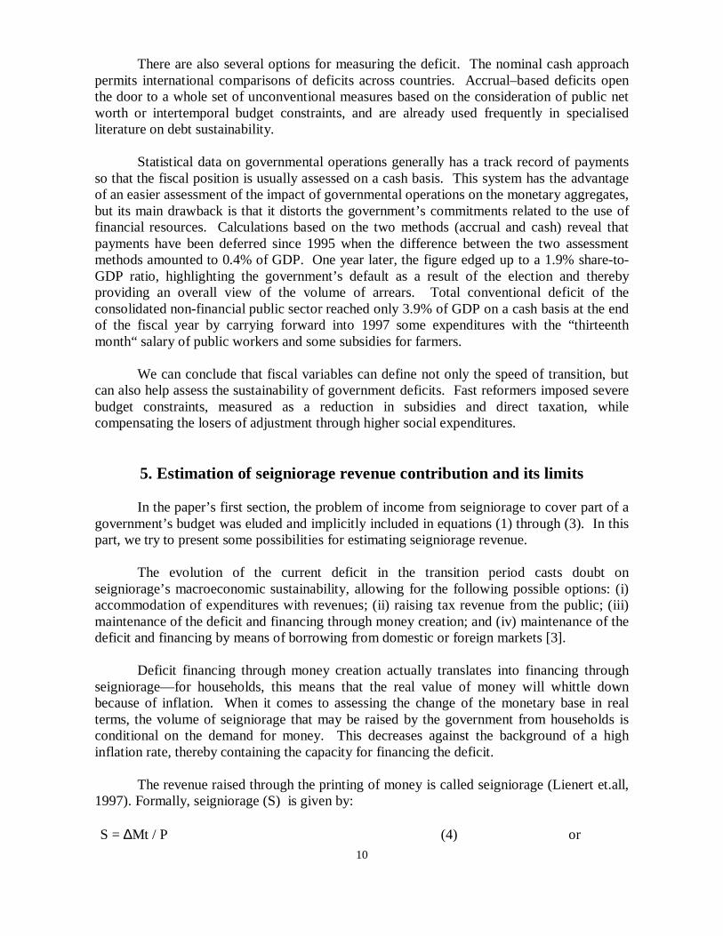
Before we close this section, it is worth looking at the relationship between externaldebt and the current account. The relationship between changes in net external debt, thecurrent account and net capital inflow (Dornbusch, 1987, p. 99) may be written as:

∆ ( NFB ) = CAD - ( NILTC + NISTPC ) (14)

where ∆ (NFB) is the change in net external debt, CAD is the current account deficit,NILTC is the net inflow of long-term capital (direct and portfolio investment), while NISTPCis the net inflow of short-term private capital.

The net inflow of private capital traditionally covers part of the current account deficit(Table 5), with net inflow of long-term capital being the dominant item (direct and residentialinvestment).

Table 5. The Romanian Balance Of Payments

bill. $1990 1991 1992 1993 1994 1995 1996 1997 1998

CAB -1.80 -1.29 -1.46 -1.23 -0.52 -1.77 -2.57 -2.14 -3.01

Net Inflow of PrivateCapital

0.14 -0.91 -0.50 0.37 -0.77 0.21 1.33 -1.11 2.11

Balance Item n.a. 0.14 0.40 0.15 0.94 0.46 0.36 1.10 0.38

Balance of Payments -1.83 -2.42 -3.28 -2.31 -1.67 -3.18 -3.99 -4.52 -4.61Before Official Borrowing

17

Up to 1995, the prevailing negative interest rates along with an underdevelopedfinancial market were discouraging short-term capital inflow. In crisis periods, domesticcapital was also fleeing abroad, avoiding the existing exchange controls in various ways.Although data on capital flight is not available, the sign of the balancing item in the balanceof payments accounts is sometimes used by the non-technical press as an indicator of suchmovements. The reversal of macroeconomic policy in 1993-1995 and in 1997-1998 with theapplication of a stabilisation programme in accordance with the IMF standby agreementcaused an increase in net capital inflow (both long-term and short-term) and, apparently, areversal of capital flight. The authorities’ change of attitude toward foreign capital (therelevant low was modified in favour of direct investment while the implementation of agradual deregulation of financial and product markets started immediately), the overall stanceof economic policy, and the 1998 programme caused an increase in private long-term capitalinflow. In addition, the increase in real interest rates and gradual deregulation of financialmarkets, along with the creation of new opportunities for short-term investment, attractedshort-term capital.

7. Can public sector deficits be sustained?

As we have seen, the persistent public sector primary deficits (excluding income fromprivatisation) during 1992-98 (with a small exception in 1993) have caused a new recordincrease in public sector debt. In addition, they have reduced the country’s national savingsratio to very small levels in comparison to previous periods and to international standards,reduced the public sector’s net worth since they are due to consumption and not publicinvestment deficits and are crowding out private investment. In fact, it is nationalinvestment—private and public investment—that has been crowded out by currentgovernment dissavings, as the table of Appendix 4 and Table 4b show. They have failed toboost the economy, casting doubt on whether a small, open economy like Romania, sufferingfrom structural impediments, can use an expansionary fiscal policy to boost output—especially during a period in which its trade partners are following restrictive policies.

Very few would now object to the view that the current fiscal situation in Romania isunsustainable, especially if we consider the recent external debt-service burden crisis in thisyear. It is so because the persistent primary deficits (generated indeed during someextraordinary--still too much prolonged--circumstances of transition, but not, however,during like in a period of war) combined with rising real interest rates may, at some point inthe future, crack the public’s confidence, and hence create a crisis with unforeseenconsequences in the government’s ability to generate primary surpluses to repay the existingdebt (e.g. capital flight) (Spaventa, 1988).

To see what the dynamics of debt accumulation involve, we can solve equation (3)recursively to obtain

d T = d 0 v T + Σ (π m – b m ) v T – m (m = 1, 2, …, T) (15)

where: v = ( 1 + i* + p ) / ( 1 + q + p ), while it has been assumed, in order tosimplify calculations, that the real effective interest rate, i* , the real growth rate, q, and thechange in the GDP deflator, p, are constant: i* t = i* , q t = q , p t = p. Using equation (15) we

18

can predict the debt to GDP ratio for some future moment T, making assumptions about therelevant parameters. A high real growth rate relative to the effective real interest rate tends toreduce the debt to GDP ratio, d, while persistent primary deficits net of (real) central bankfinancing tends to increase it. We consider it useful to simulate the evolution of public sectordebt for the next ten years using past parameter values that conform to the data in Table 1.The simulation output is presented in Table 6.

Romania’s determination to reduce its inflation rate in order to stabilise its economyand achieve the conditions to be accepted into the EU in the future restricts its ability toincrease the direct financing of budget deficits by NBR (as we already analysed in this paper)and also implies that (real) interest rates will have to tend to European levels. A rather safeand helpful assumption to make is that the growth rate q will be equal to the average effectivereal interest rate i* on public debt, although it looks to be in contrast to past experience. Wecan see from Table 1 that only in 1997 was i* small, 6%, which is already plausible for thegrowth rate. This assumption can be justified only when the following events happen: a rapidincrease in marginal real interest rates on government borrowing with short-term newgovernment borrowing and high real interest rates prevailing world-wide. It also has atheoretical appeal--it corresponds to the optimum growth theory's “golden rule ofaccumulation” [5]. Under the assumption q = i* , equation (15) becomes:

d T = d 0 + Σ (π m – b m ) (16)

If, for instance, the 1990-1998 average π – b, which was equal to 0.3%, is assumed toprevail during the next decade, then taking into account that d 0 = d 1999 = 1, thecorresponding ratio at the end of the next decade will be only 1.03. Another example: if the1996 average π – b, which was equal to 1.7%, is assumed to prevail during the next decade,then the corresponding ratio at the end of the next decade will be only 1.17. That is, the debtto GDP ratio will be 17% higher than it is today. Similarly, the corresponding ratio, d T , for avery large T will tend to infinity. In fact, d T will always tend to infinity for a very large T,unless the “average” future primary deficit is zero. An interesting, and empirically appealing,case arises, when the primary deficit is positive but declining. It can be shown (using the so-called d’Alambert’s theorem on the convergence of infinite series) that d T will converge toan infinite limit for a very large T, if the primary deficit, π – b, is declining at a constant rate.If q > i* , it can be shown from equation (15) that d T will always be bounded, provided thatprimary deficits remain bounded. In the special case where the primary deficit, π – b, isconstant, d T will converge to ( π – b ) / ( 1 – v ) for a very large T. It should be noted,however, that this limit will be a very large one (and may not be practically sustained). Forinstance, if π – b remains at the 1996 level for reasonable values of q and i* (7.1% for q, as itwas in 1996, and 6.0% for i* , as it was in 1997), d T will be close to 4.00, which is a veryhigh debt to GDP ratio – either by historical or by international standards. Finally, if q < i*the debt to GDP ratio increases without limit [6].

19

Table 6. The Simulation of Debt Evolution for Ten Years

Time Horizon( d 0 = 100 )

The Value ofParameters,

as in theYear*):

Value ofIndicator v** )

5 Years 10 Years1995 1.204 239 585

1996 1.317 388 1519

1997 1.054 111 124

1998 1.227 258 695

* ) See Table 1 (Excluding General Government Proceeds from Privatisation) * * ) See Equation (15)

7. Conclusions

The main conclusions of the paper are the following:

1) The record increase in the public debt to GDP ratio of the transition period is due toa very large increase of social consumption expenditures without a parallel increase in taxrevenue;

2) Record primary deficits occurred during election years (1992 and 1996), indicatingthe presence of a political business cycle;

3) Real average effective interest rates on central government debt were negative forsome years (1993 and 1994) but are increasing and probably stabilising;

4) There were many oscillations in the evolution of current account deficits relative toGDP and in public sector deficits in the background of a severe decrease in savings andinvestment (both private and governmental). Many times, they were non-correlated throughthe operation of various crowding out mechanisms;

5) High public sector consumption deficits should not continue. The country’s savingsratio is now the lowest in the European area despite a relatively constant household savingsratio, while a rapidly growing public debt may crack public confidence and lead to capitalflight;

6) a better correlation between fundamental macroeconomic indicators and includingpressures that come from international financing institutions, as appears to be the trend inrecent years, will be necessary in order to ensure the sustainability of public sector debt andthe credibility of the Romanian economy for the future.

Appendix 1

20

t

1990199119921993

1994199519961997

1998

.dtb_d%t100

37.41917.4

20.620

27.432.8

31.8

.dExb_d%t100

37.416.516.1

18.217.823.627.4

25.4

.dInb_d%t100

002.41.3

2.42.33.85.4

6.4

.dtb_L%t100

4.618.328.429.2

2225.435.936.7

39.2

.dExb_L%t100

4.618.324.727.1

19.522.530.930.7

31.3

.dInb_L%t100

003.72.1

2.52.956

7.9

dtb_d – Gross Country’s Debt to GDP Ratio, in USDdExb_d – Gross External Debt to GDP Ratio, in USDdInb_d – Gross Internal Public Debt to GDP Ratio, in USDdtb_L – Gross Country’s Debt to GDP Ratio, in LeidExb_L – Gross External Debt to GDP Ratio, in LeidInb_L – Gross Internal Public Debt to GDP Ratio, in Lei

21

Appendix 2

The Fiscal Position of a Selection of Transition Countries, 1990 - 98

Bulgaria Czech Croatia Poland Romania Russian Slovakia Slovenia

Hungary

Republic Federation1990 –8.5 –0.2 ... 3.1 0.3 ... –0.2 –0.3 0.41991 –3.8 –2.1 ... –3.8 –1.9 –13.9 –3.8 2.6 –4.9

Government 1992 –5.8 –0.2 ... –6.0 –4.4 –5.5 –2.8 0.3 –6.7Budget Budget as 1993 –11.0 0.1 0.2 –2.8 –2.6 –9.9 –6.2 0.3 –5.6

Deficit to GDP 1994 –6.5 0.9 0.6 –2.7 –4.2 –11.4 –5.2 –0.2 –7.4% 1995 –6.6 0.5 –0.8 –2.6 –4.1 –5.5 –1.6 0.0 –2.4

1996 –10.9 –0.1 –0.1 –2.5 –4.9 –8.1 –4.4 0.3 –1.91997 –3.7 –1.0 –0.9 –1.3 –3.6 –7.3 –5.7 –1.1 –4.01998 1.3 –1.6 0.9 –2.5 –3.1 –5.0 –2.7 –0.6 –5.4

Source: NBR data, Annual Report for 1998, p. 28.

22

Appendix 3

Consolidated General Government Balance (IMF adjustments)(in Percent of GDP)

1990 1991 1992 1993 1994 1995 1996 1997 1998 1999 1999Half Program

TOTAL REVENUE 39.8 41.9 37.4 33.9 32.1 32.1 29.9 30.6 35.0 42.3 33.8 Current 39.5 38.9 36.6 33.6 31.9 32.0 29.8 29.4 32.6 39.4 33.5 A. Tax 35.5 33.2 33.5 31.3 28.2 28.8 26.9 26.7 30.9 37.9 31.2 A1. Direct Tax 22.7 23.7 25.0 21.6 20.1 19.6 17.9 16.9 17.8 23.9 18.4 Profit Tax 7.1 5.1 5.3 3.8 3.8 3.9 3.3 4.3 3.3 3.9 2.4 Tax on Salaries 6.8 7.6 7.6 6.6 6.5 6.4 6.1 5.6 5.5 6.8 4.8 Social Security 7.9 10.0 10.3 9.3 7.9 7.9 7.5 6.6 8.7 11.0 8.9 Contributions Other 1.0 1.1 1.8 2.0 1.9 1.4 1.0 0.4 0.4 2.2 2.3 A2. Indirect Tax 12.8 9.5 8.5 9.7 8.1 9.3 8.9 9.8 13.1 13.9 12.7 Out of Which: Excises and Oil Tax 11.8 8.3 6.9 3.7 1.6 1.5 1.4 1.7 2.5 3.4 3.7 V.A.T. 0.0 0.0 0.0 3.6 4.6 5.2 4.9 4.7 6.6 7.2 5.9 Customs Tax 0.2 1.1 1.3 1.3 1.1 1.4 1.5 1.3 1.7 1.9 1.9 Other 0.8 0.1 0.2 1.0 0.8 1.1 1.1 2.1 2.3 1.4 1.2 B. Nontax 4.0 5.7 3.1 2.3 3.7 3.2 2.9 2.7 1.7 1.6 2.4 Capital 0.3 3.0 0.7 0.2 0.1 0.1 0.1 1.2 2.4 2.6 0.0 Others 0.0 0.0 0.0 0.0 0.0 0.0 0.0 0.0 0.0 0.3 0.3TOTAL EXPENDITURES 38.7 38.7 42.0 34.2 33.9 34.7 33.8 34.2 38.3 46.1 35.9 Current 30.8 32.7 36.7 29.3 28.1 28.8 28.2 28.8 34.3 42.7 32.7 Goods and Services 12.3 13.6 14.1 12.0 12.4 12.6 11.8 10.7 12.9 16.3 10.6o/w: Wages and Salaries 7.2 7.7 7.5 6.8 6.7 6.5 6.0 4.9 5.5 7.0 4.8 Interest Payments for thePublic Debt

0.0 0.0 0.2 0.9 1.4 1.4 1.7 3.4 5.4 6.1 5.4

Subsidies and Transfers 19.8 21.6 25.9 18.1 16.3 17.4 16.5 14.1 16.0 20.4 15.1 Subsidies 8.3 11.7 16.5 8.6 5.8 6.6 6.1 2.5 1.7 3.1 1.5 Transfers 11.6 9.9 9.4 9.5 10.5 10.8 10.4 11.6 14.4 17.3 13.5 Capital 7.9 6.0 4.1 4.3 5.5 5.3 5.2 4.8 3.3 3.1 2.7 Lending minus Repayments 0.0 0.0 1.1 0.5 0.2 0.6 0.3 0.6 0.6 0.3 0.2 OVERALL BALANCE (Cash-

Net of1.0 3.2 -4.6 -0.8 -2.5 -3.8 -5.5 -4.6 -5.6 -6.3 -3.0

Privatisation Receipts)OVERALL BALANCE (Cash- 1.0 3.2 -4.6 -0.4 -1.9 -2.6 -3.8 -3.6 -3.3 -3.8 -2.0Including PrivatisationReceipts) PRIMARY Balance (IncludingPrivate)

1.0 3.3 -4.4 0.6 -0.5 -1.2 -2.2 -0.1 2.1 2.8 3.4

PRIMARY Balance (ExcludingPrivate)

1.0 3.3 -4.4 0.2 -1.2 -2.4 -3.8 -1.1 -0.2 0.2 2.4

23

Appendix 4

GrossSavings

H11990 1991 1992 1993 1994 1995 1996 1997 1998 199

9

Real GDP (%) -5.6 -12.9 -8.8 1.5 3.9 7.1 3.9 -6.9 -7.3 -3.9

Current Account Balance (CAS) -8.7 -3.5 -8.0 -4.5 -1.4 -5.0 -7.3 -6.1 -7.9 -6.01.03 3.25 -4.61 -0.37 -2.40 -2.92 -4.05 -

3.91General GovernmentBalance(GGFS)

1.0 3.2 -4.6 -0.4 -1.9 -2.6 -3.8 -3.6 -3.3 -3.8

General Government Balance 8.6 6.2 -0.1 4.4 3.9 3.2 1.6 0.7 -1.8 -1.9on Current Transaction( GGFSCT)

Private Sector Gross Savings (PS) 12.6 15.3 23.9 20.6 19.8 16.6 17.2 14.4 9.8 6.2(PS=NS-GGFSCT) 26.5 22.8 23.3 18.7 20.6 9.8

National Gross Savings (NS) 21.2 21.5 23.8 24.9 23.6 19.8 18.8 15.0 8.0 4.3 (NS=PS+GGFCT)E=(Pib-Cf)/PIB 20.8 24.1 23.0 24.0 22.7 18.7 17.4 14.7 9.2 4.2

Gross Household Savings ( GHS) 1.6 3.4 4.0 7.3 7.6 5.5 … …( calculat pe baza conturilor nationale ca pondere in venitul disponibil)Private Gross Investment (PI) 22.3 22.1 27.3 24.7 19.3 19.0 20.6 17.0 14.4 7.7

Gross State Investment (GST) 7.9 6.0 4.1 4.3 5.5 5.3 5.2 4.8 3.3 2.6

Gross National Investment(NI) 30.2 28.0 31.4 28.9 24.8 24.3 25.9 21.8 17.7 10.3

24

NOTES

[1] In a recent paper published by Standard & Poor's it is shown that variousfactors have eroded the advantages of Romania’s moderate debt burden: high politicalrisk; policy slippage; and a rapid rising external debt-service burden because ofcontinued borrowing to finance budget deficits, and loss-making, state-ownedenterprises and banks (Standard and Poor’s, 1999).

[2] To estimate parameters i and a in equations (1)-(3), we used the followingrelations:

i t = Db t / D t - 1

where Db is general government interest, and respectively

a t = ( D t / D t - 1 ) [ 1 - ( CS t - 1 / CS t ) ]

with CS being the exchange rate (Lei/USD) at the end of year.

[3] Bernard Laurens and Enrique G. de la Piedra (1998) point to threepossibilities to secure government borrowing: voluntary private sector purchases ofgovernment debt in the domestic market, foreign borrowing, and forced placement ofgovernment debt--such as the creation of a “captive” market for government securitiesby forcing institutions to invest a certain share of their portfolios in such securities.

[4] It is noteworthy that the differences between the size of this indicator, afterusing this assessment method, do not affect the conclusions of our analysis. Thus,consistent with calculations made by Nina Budina (1998), gross seigniorage inRomania equalled 7.8% in 1992, 7.4% in 1993, 9.8% in 1994, 2.9% in 1995, and5.25% in 1996.

[5] Approaches to the problem of debt accumulation using differentialequations end up with an indeterminacy in the case where g = i, while the presentmethod, starting from equation (3) and solving it recursively to obtain equation (15),avoids it (OECD, 1989).

[6] This is the so-called Domar’s law.

25

REFERENCES

Barro, R. (1988): “The Ricardian Approach to Budget Deficits," NBER,Working Paper, no. 2685.

Blanchard, O. J. (1990): “Suggestion for a New Set of Fiscal Indicators,”OECD Working Paper, 79, Paris.

Budina, N., Malisyewski, W., and De Menil, G. (1998): Monetary Policy,Demand for Money and Inflation in Romania, July, Annex 3.

Buiter, W. H. (1985): “Guide to Public Sector Debt and Deficits,” EconomicPolicy, Volume 1, November.

Chalk, N. (1998): “Fiscal Sustainability with Non- Renewable Resources,”IMF Working Paper, March.

Coricelli, F. (1997): “Fiscal Policy a Long Term View,” in Fiscal Policy inTransition, in Economic Policy Initiative, 3, Forum Report of the Economic PolicyInitiative.

Croitoru, L. (1996): Politica fiscalã României în perioada 1990-1995, CEMATCuddington, J. (1996): “Analysing the Sustainability of Fiscal Deficits in

Developing Countries,” Economics Department Georgetown University, Washington,D.C.20057-1045, 3-31-1997 revision.

Dornbusch, R. (1987): Debts and Deficits, Leuven and MIT University Press.Eisner, R. (1989): “Budget Deficits: Rhetoric and Reality,” Journal of

Economic Perspectives, November.Fetherston, M.J. and Godley, W.A.H. 1978): “New Cambridge

Macroeconomics and Global Monetarism: Some Issues in the Contact of UKEconomic Policy,” in Brunner, K. and Metzler, A.H. (eds.), Public Policies in OpenEconomies, Amsterdam, North Holland.

Garcia, F. (1998): “Public Debt Sustainability and Demand for MonetaryBase,” Working Papers IMF.

Kosterna, U. (1997): “The Fiscal Policy Stance in Central and Eastern Europein Comparison to European Union Countries,” in Economic Policy Initiative, 3,Forum Report of the Economic Policy Initiative.

Laurens, B. and Piedra, E. (1998): “Coordination of Monetary and FiscalPolicies,” IMF Working Paper, WP-98-25.

Lienert, I., Marciniak, P., and Swiderski, K. (1997): “MacroeconomicAccounting and Analysis in Transition Economies,” International Monetary Fund

Olding-Smee, J. and Riley, C. (1985): Approaches to the PSBR, NationalInstitute of Economic and Social Research, August.

Rocha, R.R. and Saldanha, F. (1992): “Fiscal and Quasi Fiscal Deficits,Nominal and Real Measurement and Policy Issues,” Working Paper, WPS.

Roubini, N. and Sachs, J. (1989): “Government spending and budget deficitsin the industrial countries,” Economic Policy, April .

Spaventa, L. (1988): “Is there a public debt problem in Italy?” in Giavazzi, F.and Spaventa, L. (eds.), High Public Debt – The Italian Experience, CEPR-Cambridge University Press.

Stournaras, Y. (1990): “Public Sector Debt and Deficits in Greece: TheExperience of the 1980s and Future Prospects,” Revista di POLITICA ECONOMICA,VII-VIII, Roma, July-August.

26

Wilcox, D. (1989): ”Sustainability of Government Deficits: Implication of thePresent Value Borrowing Constraint,” Journal of Money, Credit and Banking,Volume 21, August.

* * * International Monetary Fund (1996): World Economic Outlook, Focuson Fiscal Policy, May.

* * * OECD (1989): “ Special Features, Macroeconomic Stabilisation andRestructuring Social Policy – Romania,” Economic Survey.

* * * OECD (1999): Economic Survey of Ireland, appendix 2, Paris, OCDE,1998/1999.

* * * Standard & Poor's (1999): Analysis - ROMANIA, Sovereign RatingService, August.