WP/13/261

Natural Gas, Public Investment and Debt Sustainability in Mozambique

Giovanni Melina and Yi Xiong

© 2013 International Monetary Fund WP/13/261

IMF Working Paper

African Department and Research Department

Natural Gas, Public Investment and Debt Sustainability in Mozambique1

Prepared by Giovanni Melina and Yi Xiong

Authorized for distribution by Andrew Berg, Catherine Pattillo, and Doris C. Ross

November 2013

Abstract

Mozambique has great potential in natural gas reserves and if liquefied/commercialized the sum of taxes and other fiscal revenue from natural gas will, at its peak, reach roughly one third of total fiscal revenue. Recentdevelopments in the natural resource sector have triggered a fresh round of much needed infrastructureinvestment. This paper uses the DIGNAR model to simulate alternative public investment scaling-up plans in alternative LNG market scenarios. Results show that while a conservative approach, which simply awaits LNGrevenues, would miss significant current growth opportunities, an aggressive approach would likely meetabsorptive capacity constraints and imply a much bigger (and, in an adverse scenario, unsustainable) build-up of public debt. A gradual scaling up approach represents indeed a desirable path, as it allows anticipating some,though not all, of the LNG revenue and, even in an adverse scenario, keeping public debt at sustainable levels. Structural reforms affecting selection, governance and execution of public investment projects wouldsignificantly enhance the extent to which public capital is accumulated and impact non-resource growth and, ultimately, debt sustainability.

JEL Classification Numbers: E6; Q32 Keywords: Natural resources; Debt sustainability, Public investment, Mozambique, DIGNAR

Author’s E-Mail Addresses: giovanni.melina.1@city.ac.uk; yxiong@imf.org

1 Comments and suggestions by Andy Berg, Iyabo Masha, Cathy Pattillo, Doris Ross, Andrea Presbitero, Sergio Sola, Susan Yang, Felipe Zanna and seminar participants at the African Department of the IMF and at the Ministry of Finance of the Republic of Mozambique are gratefully acknowledged. This working paper is part of a research project on macroeconomic policy in low-income countries supported by U.K.’s Department for International Development. All views and errors are the authors’.

This Working Paper should not be reported as representing the views of the IMF. The views expressed in this Working Paper are those of the author(s) and do not necessarily represent those of the IMF, IMF policy, or of DFID. Working Papers describe research in progress by the author(s) and are published to elicit comments and to further debate.

Contents PageAbstract ......................................................................................................................................1 I. Introduction ............................................................................................................................3 II. Natural Gas Sector in Mozamique: An Overview ................................................................4III. Predicting LNG Revenue: The FARI model .......................................................................6IV. Public Investment in Mozambique ......................................................................................8V. The Macroeconomic Effects of Investment Scaling-Ups .....................................................9 

A. The DIGNAR Model ................................................................................................9 B. Scenarios of LNG production .................................................................................11 C. Simulation results ....................................................................................................12 D. Structural reforms: the impact of governance and project selection .......................15 

VI. Conclusion .........................................................................................................................16References ................................................................................................................................19 

Appendices

A. DIGNAR model details ...........................................................................................21 Households .......................................................................................................21 Firms ................................................................................................................23 Government......................................................................................................25 Identities and market clearing conditions ........................................................31 

B. First-order conditions ..............................................................................................31 Demand functions for tradable and non-tradable goods ..................................31 Labour supply in the tradable and non-tradable sector ....................................31 Optimizing households’ decisions ...................................................................31 Rule-of-thumb households’ decisions ..............................................................32 Non-tradable sector’s decisions .......................................................................32 Tradable sector’s decisions ..............................................................................32

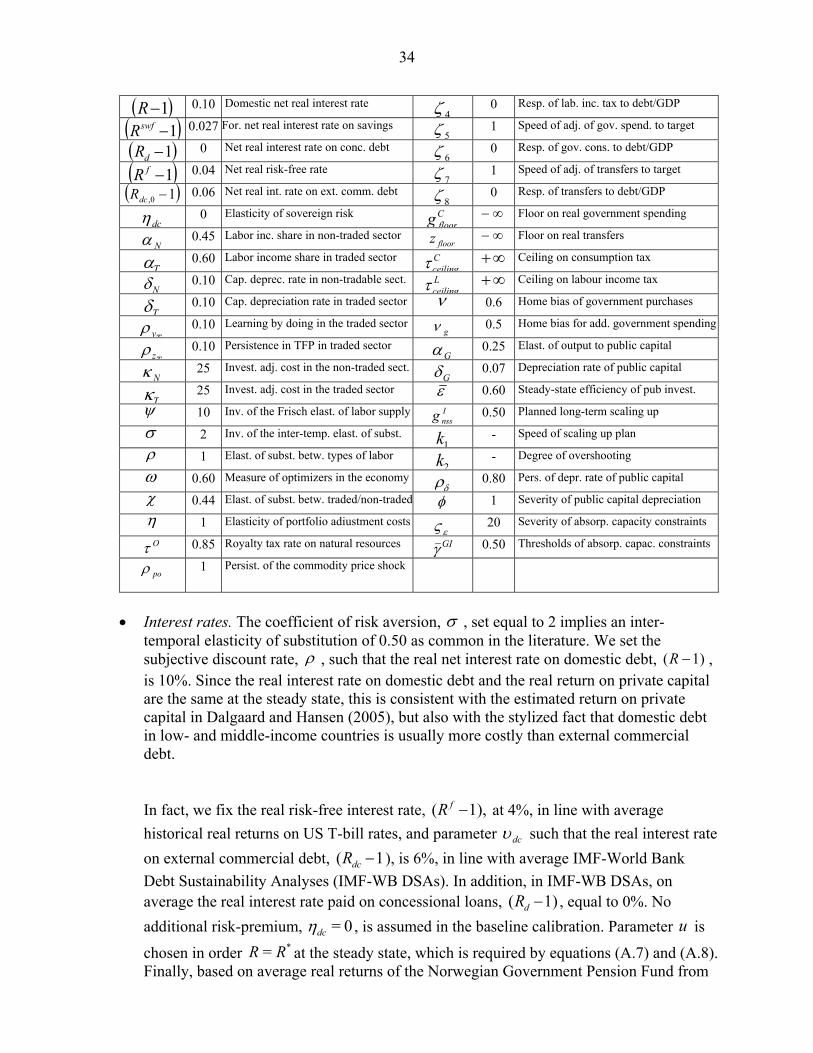
C. Calibration………………………………………………………………………...33

Tables

Table 1. Countries with World’s Largest Proven Natural Gas Reserves ...................................5 Table 2. Representative EPCC Parameters ................................................................................7 Table 3. Calibration .................................................................................................................33 

Figures

Figure 1. LNG Sector Contribution to GDP and Fiscal Revenue ..............................................8 Figure 2. Mozambique: Public Capital Expenditure, 1991-2012 ..............................................9 Figure 3. LNG Revenue Simulations in the Baseline and Adverse Scenarios. .......................12 Figure 4. Public Investment Scaling-Ups and Growth Outcomes. ..........................................13 Figure 5. Fiscal Consequences of Public Investment Scaling-Ups. .........................................14 Figure 6. The Effects of Improvements in Project Selection and Better Governance and Execution .................................................................................................................................16

3

I. INTRODUCTION

Mozambique is expected to become a major natural gas producer and liquefied natural gas (LNG) exporter in Sub-Saharan Africa. Oil companies have discovered tremendous natural gas reserves in the Rovuma Basin off the northern coast of the country. According to the business plans, liquefaction and transportation facilities are to be built, and by mid-2020s Mozambique would be exporting tens of million tons of LNG to the rest of the world, in turn bringing in billions of dollars of revenue back to the country each year. As is shown in this paper, developments in the natural gas sector will transform the landscape of the Mozambican economy. According to the results of the Fiscal Analysis of Resource Industries (FARI) model, if the LNG projects materialize as planned, LNG will become Mozambique’s single largest exporting sector and contribute up to around one third of fiscal revenue.

Although LNG production is not projected to start until around 2020, Mozambique would see the impact of the LNG sector on the economy much sooner. In anticipation of future LNG revenues, the government expects to have easier access to financing and to be able to expand its public investment program before LNG production starts. Public investment can help close the infrastructure gaps, positively impacting productivity and hence non-LNG output and growth. This, in principle, should allow the rest of the economy to benefit from the LNG sector boom.

However, investment scaling-up has its limits. The level of public debt increases along with investment scaling-up. As a result, if public investment is scaled up too quickly, debt levels will skyrocket to the extent that it may destabilize the economy. Moreover, if public investment increases too quickly, the degree of inefficiency is likely to increase as investment will more likely bump into absorptive capacity constraints and hence a bigger part of investment expenditures would be wasted. This would also impact debt sustainability.

We analyze these issues and evaluate the costs and benefits of public investment scaling-up through the lens of the “Debt, Investment, Growth and Natural Resources” (DIGNAR) model. This model is designed to analyze the public investment and growth nexus together with debt sustainability and natural resource revenue management in developing countries. The framework is based on a Dynamic Stochastic General Equilibrium (DSGE) model developed by Melina et al. (2013) at the Research Department of the IMF. DIGNAR merges the model for debt sustainability analysis in Buffie et al. (2012) with that for natural resource revenue management in Berg et al. (2013) and International Monetary Fund (2012), and introduces some additional features such as a public investment path that can potentially exhibit frontloading – the degree of which can be parameterized – and fiscal buffers, the lower bound of which represents a policy choice. As the analysis of the Mozambican case has a medium- to long-run horizon, we calibrate the model at an annual frequency.

Model parameters are calibrated to fit the context of Mozambique. We use the model to simulate output and public debt paths under different public investment strategies. These strategies include a conservative approach, in which public investment does not increase at all before LNG production starts; a gradual approach, in which public investment rises gradually before LNG production starts; and an aggressive approach, in which investment increases massively early on.

4

The modeling framework also allows us to assess the impact on output and debt of uncertainties that typically surround LNG markets. We compare between two scenarios: a baseline scenario in which LNG production is on track and LNG prices follow a path observable in normal times, and an adverse scenario in which average LNG production is down by 20 percent and there are negative LNG price shocks of a size typically observable in oil and gas market crises.

Our main results suggest that public investment has a great potential of turning LNG wealth into higher non-resource growth in Mozambique. More specifically, a gradual public investment scaling-up anticipating some but not all future LNG revenue would be appropriate in order to balance Mozambique’s tremendous infrastructure investment needs with the uncertainty regarding LNG production/revenue. In contrast, due to absorptive capacity constraints, an aggressive approach is not likely to yield tangibly better growth outcomes and poses threats to debt sustainability.

The remainder of the paper is structured as follows. Section II provides an overview of LNG developments in Mozambique. Section III presents the results of the FARI model in projecting LNG revenue. Section IV provides some background on Mozambican public investment. Section V presents the DIGNAR model and its predictions on the macroeconomic effects of public investment scaling-ups. Section VI concludes. The model equilibrium conditions and calibration are appended to the paper.

II. NATURAL GAS SECTOR IN MOZAMIQUE: AN OVERVIEW

Mozambique has long been recognized to have potential in hydrocarbon resources. The Pande and Temane gas fields were discovered in the 1960s, but civil unrest in the 1970s and 1980s halted in gas exploration activities. Exploration resumed slowly in the 1990s, partly reflecting low oil prices. Activity accelerated in the early 2000s as oil and natural gas prices rose globally. In 2003 Sasol, a South African oil company, carried out extensive exploration in the Pande/Temane onshore blocks in the South of the country, increasing gas reserves to 5½ trillion cubic feet (TCF). Mozambique started to export gas to South Africa through pipelines in 2004.

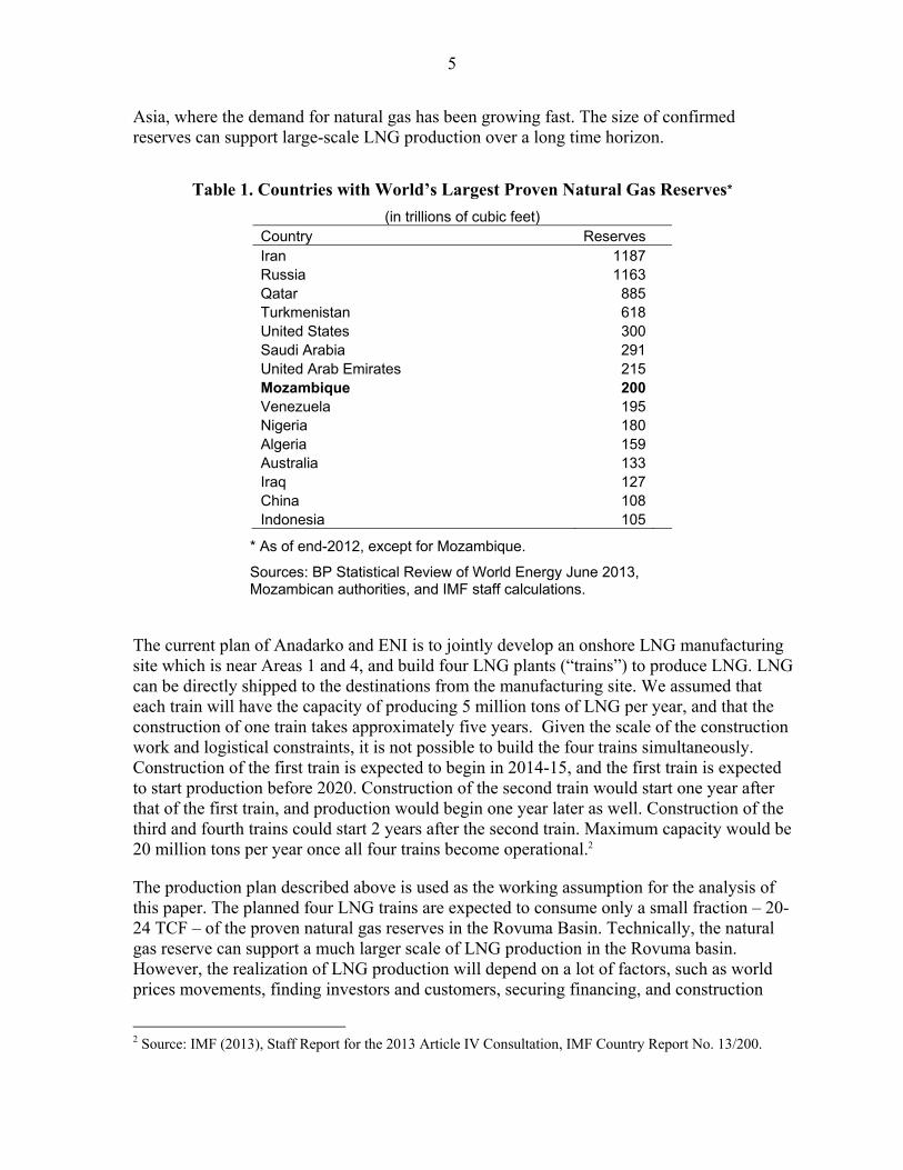
Although the early gas discoveries and commercial activities were concentrated in the South, the future of natural gas sector in Mozambique lies in the northern region. Geographic survey results show that the Rovuma basin, offshore close to the Mozambique-Tanzania border, has great potential in hydrocarbon reserves. The Mozambican government has contracted exploration and production agreements with a number of international partners since 2006. Explorations to date revealed enormous amount of recoverable natural gas reserves in offshore Areas 1 (operations led by the US-based oil company Anadarko) and 4 (operations led by the Italian oil company ENI). Total gas reserves discoveries in the two areas combined reach 200 TCF and are expected to increase further. The discoveries thus far have made Mozambique’s natural gas reserves the second largest among all sub-Saharan African countries, comparable to Nigeria’s (Table 1).

The natural gas discoveries in the Rovuma basin created the possibility for Mozambique to become a major natural gas exporter. The offshore nature and geographic location of the gas reserves made it economically feasible to liquefy and transport natural gas to South and East

5

Asia, where the demand for natural gas has been growing fast. The size of confirmed reserves can support large-scale LNG production over a long time horizon.

The current plan of Anadarko and ENI is to jointly develop an onshore LNG manufacturing site which is near Areas 1 and 4, and build four LNG plants (“trains”) to produce LNG. LNG can be directly shipped to the destinations from the manufacturing site. We assumed that each train will have the capacity of producing 5 million tons of LNG per year, and that the construction of one train takes approximately five years. Given the scale of the construction work and logistical constraints, it is not possible to build the four trains simultaneously. Construction of the first train is expected to begin in 2014-15, and the first train is expected to start production before 2020. Construction of the second train would start one year after that of the first train, and production would begin one year later as well. Construction of the third and fourth trains could start 2 years after the second train. Maximum capacity would be 20 million tons per year once all four trains become operational.2

The production plan described above is used as the working assumption for the analysis of this paper. The planned four LNG trains are expected to consume only a small fraction – 20-24 TCF – of the proven natural gas reserves in the Rovuma Basin. Technically, the natural gas reserve can support a much larger scale of LNG production in the Rovuma basin. However, the realization of LNG production will depend on a lot of factors, such as world prices movements, finding investors and customers, securing financing, and construction

2 Source: IMF (2013), Staff Report for the 2013 Article IV Consultation, IMF Country Report No. 13/200.

Table 1. Countries with World’s Largest Proven Natural Gas Reserves*

(in trillions of cubic feet) Country Reserves

Iran 1187

Russia 1163

Qatar 885 Turkmenistan 618

United States 300 Saudi Arabia 291

United Arab Emirates 215

Mozambique 200 Venezuela 195 Nigeria 180

Algeria 159 Australia 133

Iraq 127 China 108

Indonesia 105

* As of end-2012, except for Mozambique.

Sources: BP Statistical Review of World Energy June 2013, Mozambican authorities, and IMF staff calculations.

6

capacity constraints. Because of these uncertainties, we take the four-train LNG production scenario as the baseline for our analysis.

III. PREDICTING LNG REVENUE: THE FARI MODEL

We projected the contribution of the LNG sector to GDP and revenue using the Fiscal Analysis of Resource Industries (FARI) model developed by the IMF Fiscal Affairs Department (FAD), the details of which can be found in IMF (2012). The FARI model forecasts the contributions of specific mining and/or petroleum projects to fiscal revenue, balance of payment, and national accounts. Inputs to the model include production, exports, cost structure and prices assumptions, as well as fiscal regime parameters.

Calibration of the FARI model to fit the context of the Mozambican LNG projects was done by two FAD technical assistance missions to Mozambique in 2012 and 2013. Based on their results, we updated the production and cost assumptions in the model to reflect the planned four-train project as described in the previous section.

The key assumptions for the LNG projects are as follows:

LNG production is projected to start in 2020. Production in the first year is projected to be 5 million tons or a quarter of the full capacity, because only one of the four trains is expected to be operational in the first year. A second train will become operational by end-2020, boosting production to 10 million tons in 2021 and 2022. LNG production will reach the maximum capacity of 20 million tons per year in 2023.

Total investment is projected at $40 billion over the project horizon, roughly half-half split between the upstream (natural gas extraction and initial processing) and the midstream (liquefaction). On the upstream side, the cost of upfront exploration and development is expected to reach $15 billion by 2021, and another $5 billion will be invested in drilling over the project horizon to maintain gas production levels. On the midstream, the construction of the LNG plants and supporting infrastructure is projected to cost $20 billion between 2014 and 2022.

Financing for the investment will be 30 percent in equity and 70 percent in debt. Debt financing is assumed to be on commercial terms.

Separation of upstream (natural gas mining) and midstream (liquefaction). Gas liquefaction will be under a separate entity from the upstream. The upstream gas mining company will have natural gas liquefied by the LNG plants and pay service fees to the midstream company. The internal rate of return (IRR) for the midstream project is assumed at 8 percent for the purpose of determining the cost of gas liquefaction.

LNG prices will follow oil price movements over the medium term. We obtained oil price projections from the IMF April 2013 World Economic Outlook. A slope coefficient of 0.14 is applied to obtain medium term natural gas price projections. The LNG price is assumed to be constant in real terms over the long run from 2018 onwards.

7

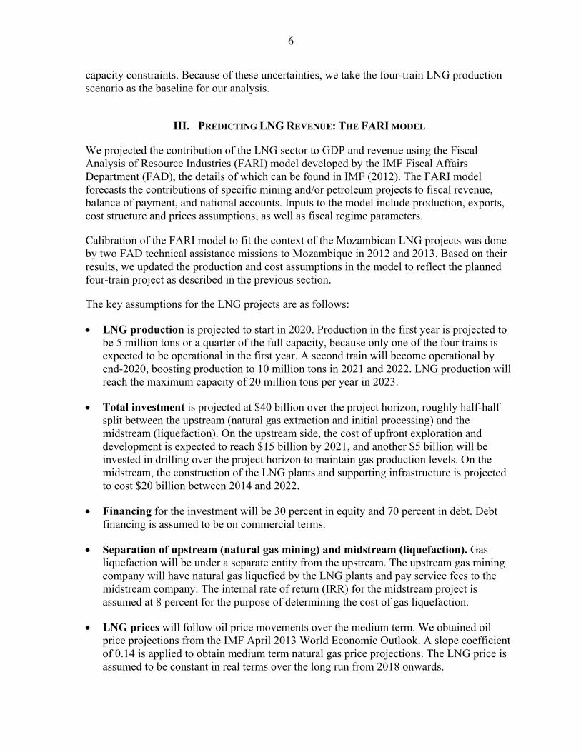
Fiscal regime. The fiscal regime for the natural gas activities comprises three main elements: a production tax (royalty), a production sharing agreement, and a corporate income tax levied on the profits of the contractors. Detailed fiscal rules are set out in the Exploration and Production Concession Contracts (EPCCs) negotiated between the government and the contractors. The EPCCs for Anadarko and ENI’s explorations have both been signed in 2006. Representative parameters from existing EPCCs are used to calibrate the FARI model (Table 2). The terms of the two specific EPCCs remain confidential.

The R-factor is a cost recovery parameter that determines the share of profit gas earned by the government. It is calculated as the ratio of the concessionaire’s cumulative cash inflows, net of operating costs and tax, to its cumulative capital expenditures. According to the representative setting, the government’s production share starts at 10 percent, and will gradually increase to 60 percent as the R-factor increases.

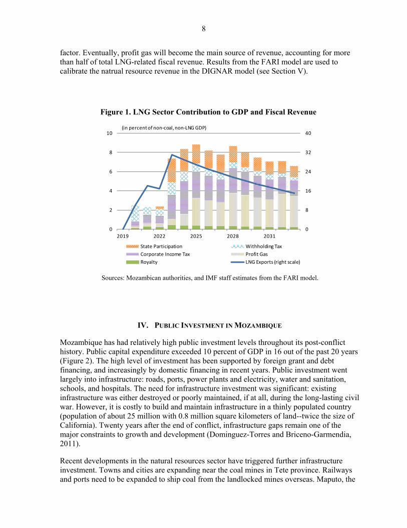
FARI model results show that the natural gas projects would bring in significant economic benefits to Mozambique. Exports peak at 30 percent of non-oil GDP, and the sum of taxes and other fiscal revenue from natural gas, at its peak, reach 9 percent of non-oil GDP, or roughly one third of total fiscal revenue (Figure 1). The government’s share is projected to be small in the first few years, when gas production volume is small and the bulk of the revenue is used to cover costs. Revenue is expected to surge in 2023 when all four LNG trains become operational, and would gradually increase afterwards. The composition of revenue also changes over the project horizon. At first the main source of revenue is subcontractor withholding tax. Corporate income tax and payoff from public enterprise participation will pick up a few years after the projects start. Revenue from EPCC production sharing will be small at the beginning, but the share of profit gas will increase gradually along with the R-

Table 2. Representative EPCC Parameters

Tax Tax Rate

Royalty 2%

Cost recovery limit 65%

R-Factor Share

Profit Petroleum / Gas 1.0 10%

2.0 20%

3.0 30%

4.0 50%

> 4.0 60%

Corporate Income Tax

In first 8 years from production start 24%

After first 8 years 32% Dividend withholding tax 10%Subcontractor withholding tax 20%

Source: National Petroleum Institute of Mozambique (INP).

8

factor. Eventually, profit gas will become the main source of revenue, accounting for more than half of total LNG-related fiscal revenue. Results from the FARI model are used to calibrate the natrual resource revenue in the DIGNAR model (see Section V).

IV. PUBLIC INVESTMENT IN MOZAMBIQUE

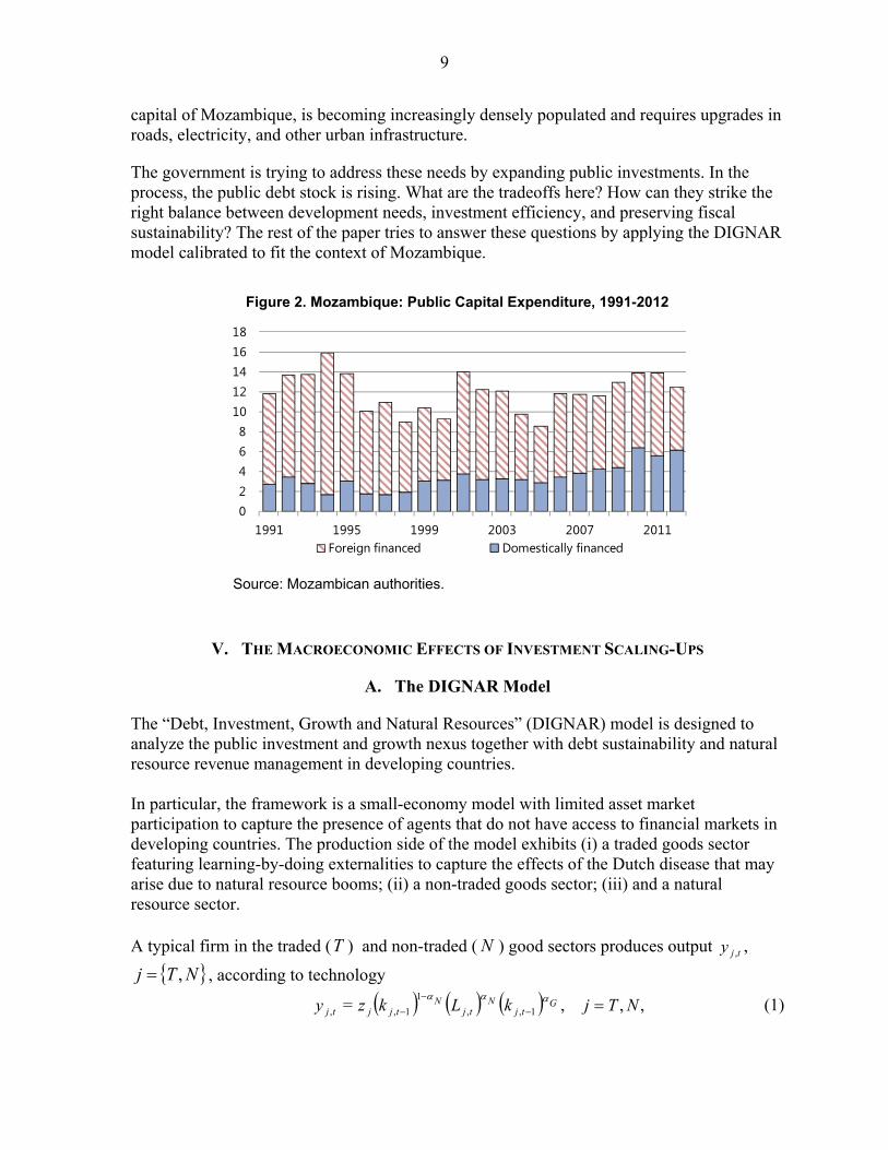
Mozambique has had relatively high public investment levels throughout its post-conflict history. Public capital expenditure exceeded 10 percent of GDP in 16 out of the past 20 years (Figure 2). The high level of investment has been supported by foreign grant and debt financing, and increasingly by domestic financing in recent years. Public investment went largely into infrastructure: roads, ports, power plants and electricity, water and sanitation, schools, and hospitals. The need for infrastructure investment was significant: existing infrastructure was either destroyed or poorly maintained, if at all, during the long-lasting civil war. However, it is costly to build and maintain infrastructure in a thinly populated country (population of about 25 million with 0.8 million square kilometers of land--twice the size of California). Twenty years after the end of conflict, infrastructure gaps remain one of the major constraints to growth and development (Dominguez-Torres and Briceno-Garmendia, 2011).

Recent developments in the natural resources sector have triggered further infrastructure investment. Towns and cities are expanding near the coal mines in Tete province. Railways and ports need to be expanded to ship coal from the landlocked mines overseas. Maputo, the

Figure 1. LNG Sector Contribution to GDP and Fiscal Revenue

Sources: Mozambican authorities, and IMF staff estimates from the FARI model.

0

8

16

24

32

40

0

2

4

6

8

10

2019 2022 2025 2028 2031

State Participation Withholding Tax

Corporate Income Tax Profit Gas

Royalty LNG Exports (right scale)

(in percent of non-coal, non-LNG GDP)

9

capital of Mozambique, is becoming increasingly densely populated and requires upgrades in roads, electricity, and other urban infrastructure.

The government is trying to address these needs by expanding public investments. In the process, the public debt stock is rising. What are the tradeoffs here? How can they strike the right balance between development needs, investment efficiency, and preserving fiscal sustainability? The rest of the paper tries to answer these questions by applying the DIGNAR model calibrated to fit the context of Mozambique.

V. THE MACROECONOMIC EFFECTS OF INVESTMENT SCALING-UPS

A. The DIGNAR Model

The “Debt, Investment, Growth and Natural Resources” (DIGNAR) model is designed to analyze the public investment and growth nexus together with debt sustainability and natural resource revenue management in developing countries. In particular, the framework is a small-economy model with limited asset market participation to capture the presence of agents that do not have access to financial markets in developing countries. The production side of the model exhibits (i) a traded goods sector featuring learning-by-doing externalities to capture the effects of the Dutch disease that may arise due to natural resource booms; (ii) a non-traded goods sector; (iii) and a natural resource sector. A typical firm in the traded (T ) and non-traded ( N ) good sectors produces output tjy , ,

NTj , , according to technology

,,,= 1,,

1

1,, NTjkLkzy Gtj

Ntj

Ntjjtj

(1)

Figure 2. Mozambique: Public Capital Expenditure, 1991-2012

Source: Mozambican authorities.

02468

1012141618

1991 1995 1999 2003 2007 2011Foreign financed Domestically financed

10

where jz is a total factor productivity scale parameter, tjk , is end-of-period private capital,

tjk , is end-of-period public capital, N is the labor share of sectoral income and G

represents the output elasticity with respect to public capital. The model also features inefficiencies and absorptive capacity constraints for public investment, and a time-varying depreciation rate of public capital to capture lack of maintenance, in line with the empirical literature for developing economies (see Gupta et al. 2011, among others). Dominguez-Torres and Briceno-Garmendia (2011) estimated that out of Mozambique’s $664 million expenditure per year on infrastructure during the late 2000s, as much as $204 million was lost to inefficiencies annually.

To reflect this, effective investment, – where is the percent deviation

of public investment from its initial steady state, – is given by

(2)

where represents steady-state efficiency and governs the efficiency

of the portion of public investment exceeding threshold , in terms of percent deviation

from the initial steady state. In particular, we assume that takes the following

specification:

(3)

In other words, if government investment expenditure deviates from the initial steady state

more than , the efficiency of the additional investment decreases to an extent proportional to the size of the deviation. This mechanism captures absorptive capacity constraints in developing countries. The severity of absorptive capacity constraints is measured by parameter .

The law of motion of public capital is

(4)

where is a time-varying depreciation rate of public capital, which captures the idea that

lack of maintenance shortens the life of existing capital. Details on how is modeled are

provided in Appendix A. The path of public investment scaling-ups is chosen according to the country’s plans and/or to assess alternative scenarios. Public investment can be frontloaded and the degree of the frontloading is linked to the degree of investment inefficiency.

GItt

Ig ~ 1I

ItGI

t g

g

Ig

gtI

gtI if t

GI GI

1GI g I t

GI 1 tGI

GI

g

I if tGI >

GI

,

0,1 (0,1]GItGI

I

tg

gtI = exp t

GI GI

.

GI

0,

,~1= 1,,, ttGtGtG gkk

tG ,

tG ,

11

As far as fiscal policy is concerned, the model has a fund where any positive difference between inflows (including natural resource revenue) and outflows (including investment expenditures) are saved and the lower bound of this fund is a policy choice. The fund is drawn down when such a difference is negative. However, when the fund reaches a chosen lower bound, then one or more fiscal instruments react to close it either instantaneously or by temporarily allowing accumulation of public debt and satisfying the government intertemporal budget constraint in the long run. In the case of Mozambique – where natural resource exploitation is a recent phenomenon and virtually no fiscal buffers have been yet accumulated – we set a lower bound of zero for the fund, which effectively becomes a non-negativity constraint for government assets. The model allows four fiscal instruments to close the fiscal gap (consumption tax, labor income tax, government consumption and government transfers). For simplicity, where needed, we allow only the consumption tax to stabilize debt in the long run and leave the other instruments at their initial steady state. Although the use of other instruments, combined or in isolation, imply somewhat different macroeconomic dynamics, the bottom-line of the results outlined below is robust to such choices. For full details of the model, the derivation of equilibrium conditions, and calibration see the Appendix.

B. Scenarios of LNG production

Natural resource markets are typically surrounded by substantial uncertainty. One big source of uncertainty is the price volatility which characterizes commodity markets. However, non-renewable natural resources are also subject to exhaustibility, i.e. to the fact that the endowment of a particular natural resource will be wiped out completely at a certain point in the future. In addition, there may be cases in which, while the endowment of a natural resource has not been exhausted, market conditions may make its extraction and distribution unfeasible or un-economical and, as a consequence, its production stops or considerably diminishes. This uncertainty is reflected in the revenue that the government may raise from natural resources. Although in many cases natural resource sector output is also dependent on public investment, it is not the case for Mozambique because the LNG sector is mostly offshore and does not depend on any public infrastructure.

In order to show the consequences of shocks to LNG revenue in the Mozambican case, we analyze two scenarios that we depict in Figure 3:

12

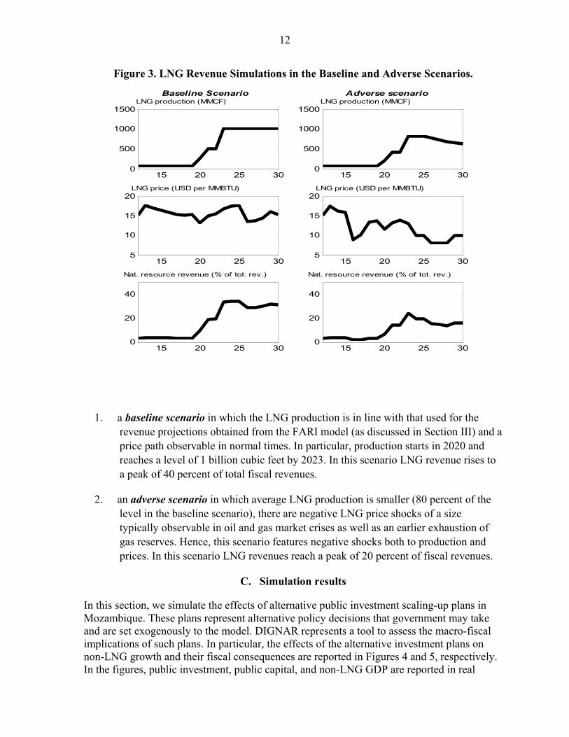
Figure 3. LNG Revenue Simulations in the Baseline and Adverse Scenarios.

1. a baseline scenario in which the LNG production is in line with that used for the revenue projections obtained from the FARI model (as discussed in Section III) and a price path observable in normal times. In particular, production starts in 2020 and reaches a level of 1 billion cubic feet by 2023. In this scenario LNG revenue rises to a peak of 40 percent of total fiscal revenues.

2. an adverse scenario in which average LNG production is smaller (80 percent of the level in the baseline scenario), there are negative LNG price shocks of a size typically observable in oil and gas market crises as well as an earlier exhaustion of gas reserves. Hence, this scenario features negative shocks both to production and prices. In this scenario LNG revenues reach a peak of 20 percent of fiscal revenues.

C. Simulation results

In this section, we simulate the effects of alternative public investment scaling-up plans in Mozambique. These plans represent alternative policy decisions that government may take and are set exogenously to the model. DIGNAR represents a tool to assess the macro-fiscal implications of such plans. In particular, the effects of the alternative investment plans on non-LNG growth and their fiscal consequences are reported in Figures 4 and 5, respectively. In the figures, public investment, public capital, and non-LNG GDP are reported in real

15 20 25 300

500

1000

1500LNG production (MMCF)

15 20 25 305

10

15

20LNG price (USD per MMBTU)

15 20 25 300

20

40

Nat. resource revenue (% of tot. rev.)

15 20 25 300

500

1000

1500LNG production (MMCF)

15 20 25 305

10

15

20LNG price (USD per MMBTU)

15 20 25 300

20

40

Nat. resource revenue (% of tot. rev.)

Baseline Scenario Adverse scenario

13

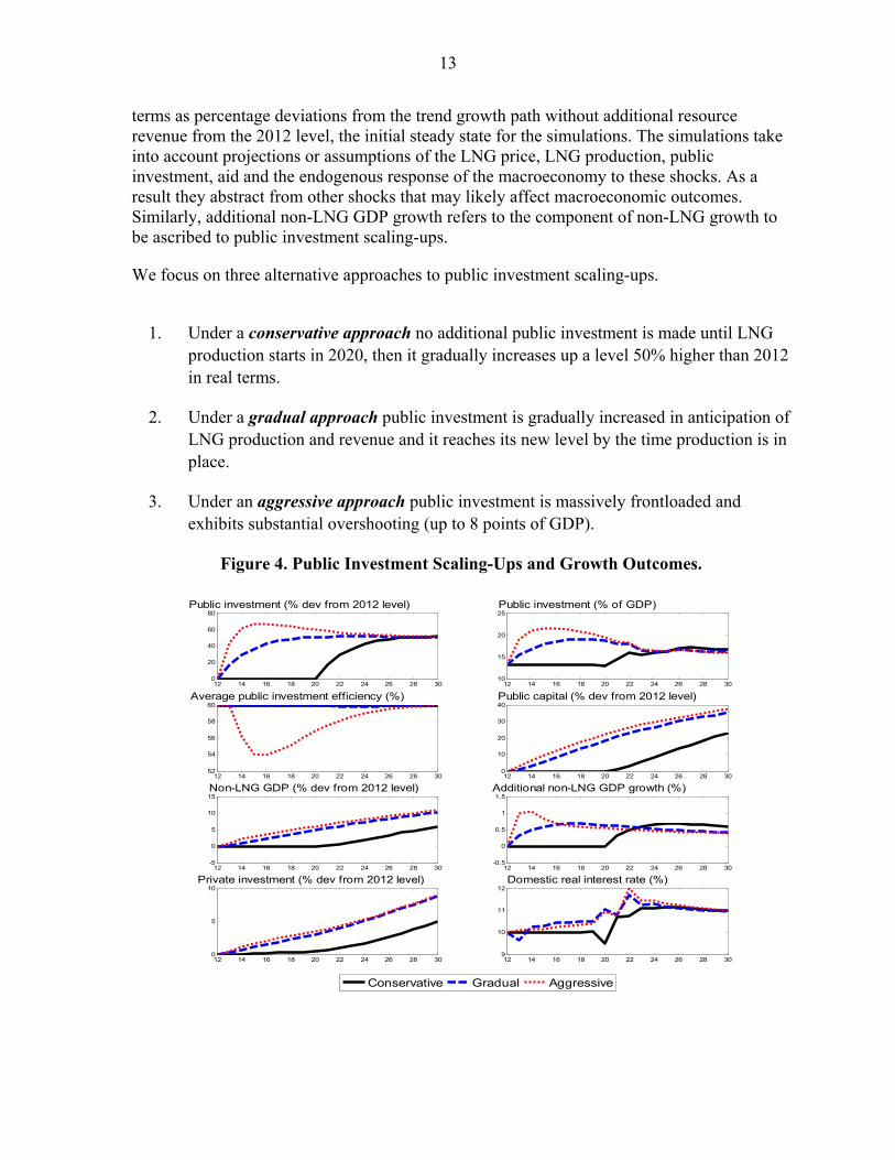
terms as percentage deviations from the trend growth path without additional resource revenue from the 2012 level, the initial steady state for the simulations. The simulations take into account projections or assumptions of the LNG price, LNG production, public investment, aid and the endogenous response of the macroeconomy to these shocks. As a result they abstract from other shocks that may likely affect macroeconomic outcomes. Similarly, additional non-LNG GDP growth refers to the component of non-LNG growth to be ascribed to public investment scaling-ups.

We focus on three alternative approaches to public investment scaling-ups.

1. Under a conservative approach no additional public investment is made until LNG

production starts in 2020, then it gradually increases up a level 50% higher than 2012 in real terms.

2. Under a gradual approach public investment is gradually increased in anticipation of LNG production and revenue and it reaches its new level by the time production is in place.

3. Under an aggressive approach public investment is massively frontloaded and exhibits substantial overshooting (up to 8 points of GDP).

Figure 4. Public Investment Scaling-Ups and Growth Outcomes.

12 14 16 18 20 22 24 26 28 300

20

40

60

80Public investment (% dev from 2012 level)

12 14 16 18 20 22 24 26 28 3010

15

20

25Public investment (% of GDP)

12 14 16 18 20 22 24 26 28 3052

54

56

58

60Average public investment efficiency (%)

12 14 16 18 20 22 24 26 28 300

10

20

30

40Public capital (% dev from 2012 level)

12 14 16 18 20 22 24 26 28 30-5

0

5

10

15Non-LNG GDP (% dev from 2012 level)

12 14 16 18 20 22 24 26 28 30-0.5

0

0.5

1

1.5Additional non-LNG GDP growth (%)

12 14 16 18 20 22 24 26 28 300

5

10Private investment (% dev from 2012 level)

12 14 16 18 20 22 24 26 28 309

10

11

12Domestic real interest rate (%)

Conservative Gradual Aggressive

14

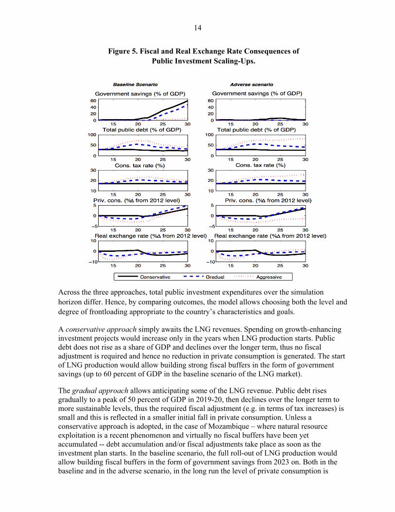
Figure 5. Fiscal and Real Exchange Rate Consequences of Public Investment Scaling-Ups.

Across the three approaches, total public investment expenditures over the simulation horizon differ. Hence, by comparing outcomes, the model allows choosing both the level and degree of frontloading appropriate to the country’s characteristics and goals.

A conservative approach simply awaits the LNG revenues. Spending on growth-enhancing investment projects would increase only in the years when LNG production starts. Public debt does not rise as a share of GDP and declines over the longer term, thus no fiscal adjustment is required and hence no reduction in private consumption is generated. The start of LNG production would allow building strong fiscal buffers in the form of government savings (up to 60 percent of GDP in the baseline scenario of the LNG market).

The gradual approach allows anticipating some of the LNG revenue. Public debt rises gradually to a peak of 50 percent of GDP in 2019-20, then declines over the longer term to more sustainable levels, thus the required fiscal adjustment (e.g. in terms of tax increases) is small and this is reflected in a smaller initial fall in private consumption. Unless a conservative approach is adopted, in the case of Mozambique – where natural resource exploitation is a recent phenomenon and virtually no fiscal buffers have been yet accumulated -- debt accumulation and/or fiscal adjustments take place as soon as the investment plan starts. In the baseline scenario, the full roll-out of LNG production would allow building fiscal buffers in the form of government savings from 2023 on. Both in the baseline and in the adverse scenario, in the long run the level of private consumption is

15

highest under the gradual approach. Private investment is crowded in by public investment. In fact, the increase in public capital increases the productivity of private capital and this translates into a higher level private investment and an increase in the domestic real interest rate.

An aggressive approach would fully anticipate future LNG revenues and increase public investment spending massively early on. However, due to absorptive capacity constraints, the higher investment spending delivers a similar build-up in the public capital stock as under the gradual approach. In fact, the fall in the efficiency on the additional public investment makes average efficiency fall by 6 percent points. The effect on the additional non-LNG growth and on the increase in private investment and consumption generated is dampened similarly. In fact only for two years non-LNG growth would be higher in with the aggressive approach; in the medium to long run the additional growth generated is similar to the gradual approach. An aggressive approach implies a much bigger build-up of public debt to 70 % of GDP in 2019-20, and would require a painful fiscal adjustment in order to service the accumulated debt, leading to a more pronounced fall in private consumption.

In addition, the aggressive approach, although the calibration assumes a mild home bias for the additional government investment (due to the fact that much of the investment goods are imported in low-income countries), leads to a relatively more pronounced appreciation of the real exchange rate (a downward movement in the charts implies an appreciation). This feeds into a relatively lower output in the traded sector, exacerbated by the presence of the learning-by-doing externality in that sector. Hence Dutch disease effects are more likely with an aggressive approach than with a gradual one.

In an adverse scenario with lower LNG production, lower LNG prices and an earlier exhaustion of gas reserves, there would be no room to build up significant fiscal buffers. Public debt would (i) not rise under the conservative approach, (ii) rise faster under a gradual approach than in the baseline; (iii) rise explosively under an aggressive approach, requiring painful and sustained fiscal adjustment without stopping the accumulation of debt. As reported in the calibration section, these simulations assume that at least half of recurrent infrastructure costs are covered by user fees. Failure to collect fees would exacerbate debt sustainability risks.

D. Structural reforms: the impact of governance and project selection

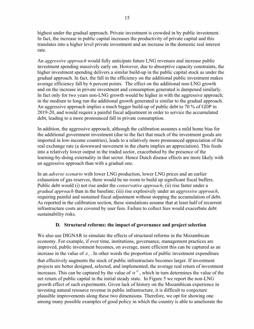
We also use DIGNAR to simulate the effects of structural reforms in the Mozambican economy. For example, if over time, institutions, governance, management practices are improved, public investment becomes, on average, more efficient this can be captured as an increase in the value of . In other words the proportion of public investment expenditure

that effectively augments the stock of public infrastructure becomes larger. If investment projects are better designed, selected, and implemented, the average real return of investment increases. This can be captured by the value of , which in turn determines the value of the net return of public capital in the initial steady state. In Figure 5 we report the non-LNG growth effect of such experiments. Given lack of history on the Mozambican experience in investing natural resource revenue in public infrastructure, it is difficult to conjecture plausible improvements along these two dimensions. Therefore, we opt for showing one among many possible examples of good policy in which the country is able to ameliorate the

t

G

16

quality of its institutions, and the fact that policies affecting the efficiency of public investment expenditures and the productivity of infrastructure projects are powerful instruments for achieving superior macroeconomic performances. In particular, we let

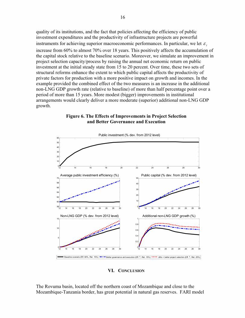
increase from 60% to almost 70% over 18 years. This positively affects the accumulation of the capital stock relative to the baseline scenario. Moreover, we simulate an improvement in project selection capacity/process by raising the annual net economic return on public investment at the initial steady state from 15 to 20 percent. Over time, these two sets of structural reforms enhance the extent to which public capital affects the productivity of private factors for production with a more positive impact on growth and incomes. In the example provided the combined effect of the two measures is an increase in the additional non-LNG GDP growth rate (relative to baseline) of more than half percentage point over a period of more than 15 years. More modest (bigger) improvements in institutional arrangements would clearly deliver a more moderate (superior) additional non-LNG GDP growth.

Figure 6. The Effects of Improvements in Project Selection and Better Governance and Execution

VI. CONCLUSION

The Rovuma basin, located off the northern coast of Mozambique and close to the Mozambique-Tanzania border, has great potential in natural gas reserves. FARI model

t

12 14 16 18 20 22 24 26 28 300

10

20

30

40

50

60Public investment (% dev. from 2012 level)

12 14 16 18 20 22 24 26 28 3058

60

62

64

66

68

70Average public investment efficiency (%)

12 14 16 18 20 22 24 26 28 300

10

20

30

40

50Public capital (% dev. from 2012 level)

12 14 16 18 20 22 24 26 28 300

5

10

15Non-LNG GDP (% dev. from 2012 level)

12 14 16 18 20 22 24 26 28 300

0.2

0.4

0.6

0.8

1Additional non-LNG GDP growth (%)

Baseline scenario (Eff. 60%, Ret. 15%) Better governance and execution (Eff. , Ret. 15%) ditto + better project selection (Eff. , Ret. 20%)

17

results show that the natural gas projects can bring significant economic benefits to Mozambique, and the sum of taxes and other fiscal revenue from natural gas could, at its peak, reach 9 percent of non-oil GDP, or roughly one third of total fiscal revenue.

Recent developments in the natural resources sector have triggered a fresh round of infrastructure investment. Indeed, the need for infrastructure investment is significant. Public investment scaling-up can help unlock Mozambique’s growth potential. However, if debt-financed public investment scaled up too rapidly, it may also lead to high debt ratios or bump into efficiency constraints.

In this study, we used the DIGNAR model to simulate alternative public investment scaling-up plans in alternative LNG market scenarios. We considered three different approaches towards public investment scaling-up: a gradual approach, a conservative approach, and an aggressive approach. In sum, a gradual public investment scaling-up anticipating some but not all future LNG revenue would be appropriate given Mozambique’s infrastructure investment needs and the uncertainty regarding LNG production/revenue. The gradual approach outperforms the other two approaches under both the baseline scenario, in which the LNG project materializes as planned, and the adverse scenario, in which Mozambique suffers negative shocks to both production and prices. Under the gradual approach, public debt rises gradually in preparation of LNG production, but then declines over the longer term to more sustainable levels, even in an adverse scenario.

In comparison, a conservative approach that simply awaits LNG revenues is not desirable, because it postpones potential additional growth benefits by almost a decade. At the same time, an aggressive approach, which fully anticipates future LNG revenues and increases public investment spending massively early on, is not desirable either. In fact, the higher investment spending delivers a similar build-up in the public capital stock as under a more gradual approach. In addition, an aggressive approach implies a much bigger build-up of public debt which would become unsustainable in an adverse scenario with lower-than-planned LNG production and lower LNG prices.

Why is public investment not “the more, the merrier?” Given that LNG revenues will eventually come, why not start investing immediately so that the economy can immediately benefit? The simulation results from the model envisage two specific constraints facing Mozambique in light of the upcoming LNG revenue:

Firstly, public investment scaling-up inevitably runs into the rule of diminishing rate of return. Investment inefficiencies may arise from many fronts: poor planning, higher-than-expected costs, bad governance, corruption, supply bottlenecks, and lack of complementary infrastructure. The more investment projects that are starting at the same time, the more likely that some of them would be poorly selected, mismanaged, or run into supply bottlenecks. At some point, the cost of inefficiencies would outweigh the benefits from bringing the investment upfront.

Secondly, there are risks to the realization of natural resources wealth. History of LNG prices and experiences from other countries show that uncertainties are large in both production volume and prices of LNG. An aggressive investment scaling-up that anticipates all future LNG revenue would fully expose Mozambique to the downside

18

risks, leading to unsustainable debt path under the adverse scenario of negative shocks to LNG production and prices.

The policy implications from this study are straightforward. Mozambique needs to strike the right balance between public investment and debt sustainability. The authorities need to have an integrated investment plan to track and coordinate investment projects undertaken in different sectors and under different line ministries. Debt levels need to be monitored closely, and debt sustainability analysis should be conducted at least annually to ensure that the build-up of debt is on a sustainable path.

To overcome the risk of adverse shocks to LNG production and prices, the public investment strategy should anticipate only a portion of projected revenue from the LNG sector. The increase in debt-financed investment should be moderate such that the debt path would remain sustainable even under the adverse scenario. Mozambique should not follow the aggressive approach to public investment, under which debt stock would explode under the adverse scenario.

The paper also shows the importance of structural reforms to improve investment efficiency. In the context of Mozambique, such structural reforms include the preparation and implementation of an Integrated Investment Program that strengthens the project selection process and coordination; capacity building for project appraisal and evaluation capacity; and improving governance and execution of public investment projects. If Mozambique could improve on these fronts, in particular reducing investment inefficiency and improving the return of public capital, the public capital stock would build up more rapidly and would become more conducive to private sector growth. The end-result would be an even higher positive impact on growth, incomes and debt sustainability.

19

REFERENCES

Berg A., Portillo R., Yang S. S. and L. F. Zanna (2013). Public Investment In Resource-Abundant Developing Countries, IMF Economic Review, 61(1), 92-129.

Buffie E., Berg A., Pattillo C., Portillo R., and L.F. Zanna (2012). Public Investment, Growth

and Debt Sustainability: Putting Together the Pieces, IMF Working Paper, 12/144, Washington DC: International Monetary Fund.

Dalgaard, C. and H. Hansen (2005). The Return to Foreign Aid. Discussion Paper No. 05-04,

Institute of Economics, University of Copenhagen. Dominguez-Torres, C., and C. Briceno-Garmendia (2011). Mozambique’s Infrastructure: A

Continental Perspective, Policy Research Working Paper, 5885, Washington DC: The World Bank.

Goldberg, J. (2011). Kwacha Gonna Do? Experimental Evidence about Labor Supply in

Rural Malawi. Manuscript, Economics Department, University of Maryland. Gros, D., and T. Mayer (2012). A Soverign Wealth Fund to Lift Germany’s Curse of Excess

Savings). CEPS Policy Brief No. 280, August 28, Centre for European Policy Studies.

Gupta, S., Kangur, A., Papageorgiou, C. and A. Wane. (2011). Efficiency-Adjusted Public

Capital and Growth.” IMF Working Paper, WP/11/217. Hamilton, J. D. (2009). Understanding Crude Oil Prices, Energy Journal, Vol. 30, No. 2, pp.

179-206. Horvath, M. (2000). Sectoral Schoks and Aggregate Fluctuations. Journal of Monetary

Economics, Vol. 45, No. 1, pp. 69-106. IMF (2012). Macroeconomic Policy Frameworks for Resource-Rich Developing Countries,

Washington DC: International Monetary Fund. IMF (2013). Staff Report for the 2013 Article IV Consultation, Sixth Review Under the

Policy Support Instrument, Request for a Three-Year Policy Support Instrument and Cancelation of Current Policy Support Instrument. IMF Country Report No. 13/200.

Melina G., Yang S. S. and L. F. Zanna (2013). Debt Sustainability, Public Investment and

Natural Resources in Developing Countries, IMF Working Paper, Washington DC: International Monetary Fund.

Pritchett, L. (2000). The Tyranny of concepts: CUDIE (Cumulated, Depreciated, Investment

Effort) Is Not Capital, Journal of Economic Growth, Vol. 5, No. 4, pp. 361-384.

20

Stockman, A. C. and L. L. Tesar (1995). Tastes and Technology in a Two-Country Model of the Business Cycle: Explaining International Comovements, American Economic Review, Vol. 85, No. 1, pp. 168-185.

21

APPENDIX

A. DIGNAR model details

Households Let us assume a continuum of infinitely lived households distributed over the unit

interval. A fraction of households have access to capital markets where they can trade contingent securities and own firms. These agents are commonly referred to as financially unconstrained, optimizing or Ricardian. The remaining fraction of agents are financially constrained in that they do not own any asset, do not have any liabilities and in each period they just consume all of their income. These agents are commonly labeled as rule-of-thumb or hand-to-mouth consumers.

Let index denote optimizing households and denote rule-of-thumb households. Both types of agents consume a composite good , for , which

in turn is a constant-elasticity-of-substitution (CES) aggregate of the traded good, , which

can be produced domestically or imported, and the domestic non-traded good, . Thus, the

consumption basket reads as

(A1)

where indicates the non-traded good bias and is the intra-temporal elasticity of substitution.

Let , and be the relative prices of goods and relative price of traded

goods to composite consumption, respectively. Minimizing total consumption expenditure, subject to consumption basket (1), yields the demand functions for each good. Let the composite consumption be the numeraire of the economy and assume that the law of one price holds at the level of traded goods, then represents also the real exchange rate

(defined as the price of one unit of foreign consumption basket in terms of the domestic consumption basket). This implies, that in real terms the price of one unit of consumption is

Both types of agents provide labor services and , , to the

traded and the non-traded sector, respectively and total labor effort, , has a CES

specification to capture the fact that hours worked in the two sectors are not perfect substitutes,

(A2)

where is the steady-state share of labor in the non-traded sector and is the intra-

temporal elasticity of substitution. Let and be the real wages paid in sectors and

, respectively, and be the real wage index. Maximizing the household’s total labor

1

OPT ROTitc ROTOPTi ,=

itTc ,

itNc ,

ROTOPTiccc itT

itN

it ,=,1=

11

,

11

,

1

0>

pT ,t pN ,tT N

st pT ,t

.1=1 11,

ttN spi

tTL ,i

tNL , ROTOPTi ,=itL

ROTOPTiLLL itT

itN

it ,=,1=

11

,

11

,

1

0>

tTw , tNw ,T

N tw

22

income , subject to aggregate labor (5), yields the labor supplies for

each sector and the real wage index,

Optimizing Households A typical optimizing household seeks to maximize its inter-temporal utility function

,11

1=,

11

0=0

0=0

OPT

t

OPTOPTt

t

t

OPTt

OPTt

t

t

LcELcUE (A3)

subject to its budget constraint expressed in units of composite consumption,

(A4)

where represents the expectation at time , is the subjective discount

factor, is the pure rate of time preference, is the inverse of the inter-temporal elasticity

of substitution of consumption, is the instantaneous utility function, is the

inverse of the intra-temporal elasticity of substitution of labor supply, is the disutility weight of labor, is the tax rate on consumption, is the tax rate on labor income,

are domestic government bonds that pay units of the domestic consumption

composite at time , are liabilities towards the rest of the world that entail

repayment of units of the foreign consumption basket, and are firms’

profits in the traded and the non-traded sector, , is a tax rebate that

optimizing households are assumed to receive on the tax levied on the firms’ return on capital,3 are remittances from abroad, are government net transfers, are user fees

of public capital , and are portfolio adjustment costs associated

to foreign liabilities, where is a scaling factor and is the initial the steady-state value of private foreign liabilities.

Let be the Lagrange multiplier attached to the budget constraint (12), then

households decisions are summarized by the first-order conditions with respect to ,

, and . In addition we assume that on its foreign debt, the private sector pays a

3 The assumption made is that, because of distortions in revenue mobilization, fraction

K of the tax revenue on private capital does not enter the government flow budget constraint. Poor institutions or corruption may be the channel through which part of the revenue is lost in the process of tax collection and earned, de facto, by private agents, which we assume to belong to optimizing households. In practical

terms, this allows us to set a high enough tax rate, K , which in turn allows us to match the observed low initial private investment flow

and capital stock typical of LICs, while K can be set to match the actual revenue that the government is able to raise.

=itt Lw i

tNtNi

tTtT LwLw ,,,,

.1= 1

11

,1

, tTtNt www

OPT

tttOPT

ttOPT

ttLt

OPTtt

OPTt

OPTt

Ct bs

Rb

RLwbsbc 1

11

1

111=1

1,,1,,,, tNK

tNtTK

tTKK

tNtT krkr

,1,

OPT

ttGttt kzrms

0E 0 11

OPTt

OPTt LcU ,

OPTCt

Lt

OPTtb

OPTttbR

1t OPTtb

OPTtt bR tT , tN ,

1,,1,, tNK

tNtTK

tTKK krkr

trm tz

tGk , 22

OPTOPT

tOPTt bb

OPTb

tOPTtc OPT

tLOPTtb OPT

tb

23

constant premium over the interest rate that the government pays on external commercial debt, :

(A5)

Rule-of-Thumb Households Rule-of-thumb households have the same instantaneous utility function as optimizing

households

(A6)

and they are subject to the budget constraint (A7)

but they do not smooth consumption by solving an inter-temporal utility maximization problem. They simply consume all of their income period by period.

Aggregation

Aggregation across implies that consumption and labor are given by the weighted

average of their counterparts in both types of households: (A8)

(A9)

Similarly, aggregate privately-owned government bonds and foreign liabilities read as (A10)

(A11)

Firms

In the economy there are three sectors: (i) a non-traded good sector indexed by ; (ii) a (non-resource) traded good sector indexed by ; and a natural resource sector indexed by . We assume that the whole resource output is exported.

Non-Traded Good Sector

A typical firm in the non-traded good sector produces output according to

technology

(A12)

utdcR ,

.= , uRR tdct

,11

1=,

11

ROTt

ROTROTt

ROTt

ROTt LcLcU

,1=1 1, tGttt

ROTtt

Lt

ROTt

Ct kzrmsLwc

i

,1 ROTt

OPTtt ccc

.1 ROTt

OPTtt LLL

,OPTtt bb

. OPTtt bb

NT

O

yN ,t

yN ,t = zN kN ,t1 1N LN ,t N kG,t1 G ,

24

where is a total factor productivity scale parameter, is end-of-period private capital,

is end-of-period public capital, is the labor share of sectoral income and

represents the output elasticity with respect to public capital. There are convex costs of adjusting investment, hence, private capital evolves as

(A13)

where represents investment expenditure, is private capital depreciation in sector

, and is the investment adjustment cost parameter.

The representative non-traded good firm maximizes its discounted lifetime profits weighted by the marginal utility of consumption of optimizing households, ,

,= 1,,,,,,,0=

0,0

tNK

tNK

tNtNtNtNtNtt

tN kriLwypE (A14)

where is a tax on the return on private capital . Let

be the Lagrange multiplier associated to the law of motion of capital, with being the

sectoral Tobin’s q. Then, firms’ decisions are captured by the first-order conditions with

respect to , , and .

Traded Good Sector

Analogously to the non-traded good sector, a typical competitive firm in the non-

traded good sector produces output according to technology

(A15)

In this sector, total factor productivity, , is subject to learning by doing externalities

depending on last period’s traded good output:

(A16)

where are structural parameters and variables with no time subscripts are

steady-state values. The law of motion of sectoral private capital is perfectly analogous to that of the non-

traded good sector:

(A17)

Also the representative traded good firm maximizes its discounted lifetime profits

weighted by the marginal utility of consumption of optimizing households, ,

Nz kN ,t

kG,t N G

kN ,t = 1N kN ,t1 1 N

2

iN ,t

iN ,t1

1

2

iN ,t,

iN ,t NN N

t

K rN ,tK kN ,t1 =

1,

,,1

tN

tNtNN k

yp tNt q ,

tNq ,

LN ,t kN ,t iN ,t

yT ,t

yT ,t = zT ,t kT ,t1 1N LT ,t N kG,t1 G .

tTz ,

,= 1,1,,Ty

T

tTTz

T

tT

T

tT

y

y

z

z

z

z

0,1, TyTz

kT ,t = 1T kT ,t1 1 T

2

iT ,t

iT ,t1

1

2

iT ,t.

t

25

,= 1,,,,,,,0=

0,0

tTK

tTK

tTtTtTtTtTtt

tT kriLwysE (A18)

where is the sectoral return on private capital. Let be the

Lagrange multiplier associated to the law of motion of capital, with being the sectoral

Tobin’s q. Then, firms’ decisions are captured by the first-order conditions with respect to

, and .

Natural Resource Sector

As most natural resource production is capital intensive and much of investment in

the resource sector is financed by foreign direct investment in low income countries, it is fair to represent natural resource production as exogenous process

(A19)

where is an auto-regressive coefficient and is the resource

production shock. We make a small-open-economy assumption in that the country’s natural resource production is small relative to world production, hence the international commodity

price (relative to the foreign consumption basket), , is taken as given and evolves as

(A20)

where is an auto-regressive coefficient and is the resource

price shock. Resource GDP in units of domestic composite consumption is

(A21)

Let be the royalty rate on production. Then, the resource revenue collected each period is

(A22)

We assume that the resource output is not consumed domestically, as in low income

countries almost the entire production is typically exported.

Government

rT ,tK = mcT ,t

1,

,1

tT

tTtT k

ys tTt q ,

tTq ,

LT ,t kT ,t iT ,t

yO,t

yO

yO,t1

yO

yo

exp tyo ,

0,1yo

pO,t

,exp= 1,, pot

po

O

tO

O

tO

p

p

p

p

0,1po

.~= ,,, tOtOttO ypsy

O

.~= ,, tOtOO

tOt ypst

26

Government expenditure Government expenditure comprises government consumption, , and public

investment, . Like private consumption, also government expenditure, , is a

CES aggregate of the domestic traded good, and the domestic non-traded good, .

Thus, the government consumption basket reads as

(A23)

where is the weight given to non-tradable goods in government purchases and is

the intra-temporal elasticity of substitution, assumed to be the same as in the private consumption composite.

Minimizing total government expenditures , subject to the

government consumption basket (23), yields the demand functions for each good and the government consumption price index in terms of units of the domestic consumption

composite,

Note that is time-varying. As this paper focuses on the effects of additional government

spending in the form of government investment, we allow the weight given to non-tradable goods for the additional government spending, , to differ from its steady state value, ,

i.e.

(A24)

Public investment inefficiencies, absorptive capacity constraints and public capital depreciation

Public investment features inefficiencies and absorptive capacity constraints. To

reflect this, effective investment, – where is the percent deviation of

public investment from its initial steady state, – is given by

(A25)

where represents steady-state efficiency and governs the efficiency

of the portion of public investment exceeding threshold , in terms of percent deviation

from the initial steady state. In particular, we assume that takes the following

specification:

Ctg

Itg I

tCtt ggg

tTg , tNg ,

,1=11

,

11

,

1

tTttNtt ggg

t 0>

ptGgt = pN ,tgN ,t pT ,tgT ,t

ptG t pN

1 1 t st1

1

1 .

t

g

t =pGg pt

Ggt pGg g

ptGgt

.

GItt

Ig ~ 1I

ItGI

t g

g

Ig

gtI

gtI if t

GI GI

1GI g I t

GI 1 tGI

GI

g

I if tGI >

GI

,

0,1 (0,1]GItGI

Itg

27

(A26)

In other words, if government investment expenditure deviates from the initial steady state

more than , the efficiency of the additional investment decreases to an extent proportional to the size of the deviation. This mechanism captures absorptive capacity constraints in developing countries. The severity of absorptive capacity constraints is measured by parameter .

The law of motion of public capital is

(A27)

where is a time-varying depreciation rate of public capital, which captures the idea that

lack of maintenance shortens the life of existing capital. This is operationalized by assuming that the depreciation rate increases proportionally to the extent to which effective investment fails to maintain existing capital:

(A28)

where is the steady-state depreciation rate, parameter determines the extent to

which poor maintenance produces additional public capital depreciation while

controls its persistence.

Resource windfalls and public investment policy

Let a resource windfall be a resource revenue that is above its original steady-state

level, i.e. , and be a sovereign wealth fund (SWF) where the windfall is saved

externally. Each period, the interest income of the SWF – where is the

gross real interest rate paid on foreign government savings – enters the government’s flow budget constraint and the fund itself evolves as

(A29)

where is the initial steady-state value of the SWF, represents the total fiscal inflow,

represents the total fiscal outflow, and is a lower bound for the SWF that the

government chooses to maintain. Every period, if the fiscal inflow exceeds the fiscal outflow, more resources are saved in the SWF.4 If the sovereign wealth fund is above any fiscal

4 In order to guarantee that the SWF is not an explosive process, we assume that – in the very long run – a small autoregressive coefficient

(0,1)f is attached to ff t 1 . The model is solved at a yearly frequency for a 1000-period simulation horizon and

coefficient f is activated after the first 100 years of simulations.

gtI = exp t

GI GI

.

GI

0,

,~1= 1,,, ttGtGtG gkk

tG ,

G,t =G

GkG,t1

gt

if gt GkG,t1

G,t1 1 G if gt GkG,t1

,

G 0

0,1

OOt tt

tf

11 t

swft fRs

swfR

,,max= ,,1

t

tout

t

tintfloort s

f

s

fffffff

f tinf ,

toutf , 0floorf

floorf

28

outflow that exceeds the fiscal inflow is absorbed by a withdrawal from the fund. Whenever the lower bound constraint binds, fiscal policy reacts to cover the gap via domestic and/or external commercial borrowing, consumption and/or labor income tax adjustments, and/or adjustments in government consumption and/or government transfers. Below we explicitely define and , and we explain in greater detail how the mechanism of closing the

fiscal gap works. The resource windfall is managed using a delinked approach. Under this approach a

scaling-up path of public investment is specified as a second-order delay function,

(A30)

where is the scaling-up investment target expressed as percentage deviation from the

initial steady state, represents the speed of adjustment of public investment to the new

level and represents the degree of investment overshooting. In particular, if

, , i.e. public investment remains unchanged. If , public

investment jumps to the new steady state immediately. If , public investment is not

overshot; while increasing values of imply increasing degrees of overshooting. Parameter

, , and , can be chosen in a way commensurate to the economy’s profile of resource

revenue, absorptive capacity, resource revenue horizon and development objective, in order to make the investment scaling up sustainable from a fiscal and a more general macroeconomic point of view.

Government’s flow budget constraint and fiscal gap The government’s flow budget constraint is

(A31)

where are grants, is concessional borrowing, is external commercial borrowing,

are user fees paid on public capital (computed as fraction of recurrent costs),

and (assumed to be constant) and are the gross real interest rates paid on

concessional borrowing and external commercial borrowing, respectively. The latter incorporates a risk premium depending on the deviations of total external public debt to GDP ratio from its initial steady state,

(A32)

where is a (constant) risk-free world interest rate, is total GDP and and are

structural parameters. To captures distortions related to inefficiencies of revenue mobilization in low-income countries, we allow fraction of capital tax revenue

tinf , toutf ,

,exp2exp11= 21InssI

It gtktk

g

g

Inssg

0>1k

12 kk 0== 21 kk tgg II

t = 1k

12 = kk

2k

1k 2k Inssg

1,,1,,, 1 tNK

tNtTK

tTKK

tOttLtt

Ct krkrtLwc

1,1, tGt

swfttctttt kfRsdsdsb

tttctdcttdttttttIt

Ct

Gt fsdRsdRsbRgrszggp 1,1,111=

tgr td tcd ,

GGtfp f

dR tdcR ,

,exp= ,1,

y

dd

y

ddRR c

t

tctdcdc

ftdc

fR ty dc dc

0,1K

29

not to appear in the government budget constraint. In other words the government is unable to use these as additional sources of fiscal revenue.

The government is assumed to accept all concessional loans extended by official creditors. It is also assumed that borrowing and the amortization schedule for these loans is set exogenously. Given the path of public investment, concessional borrowing and grants, straightforward algebraic manipulation of equation (A31) allows decomposing the government’s flow budget constraint into two components: (i) the fiscal gap before any policy adjustment,

(A33)

where

(A34)

(A35)

and (ii) the policy reaction to cover the gap itself, (A36)

which entails domestic and/or external commercial borrowing, , consumption

and/or labor income tax adjustments, , and/or adjustments in

government consumption and/or government transfers, . By

combining equations (A29) and (A33), it is straightforward to see that, if , then

, i.e. the SWF absorbs any fiscal gap and no fiscal policy adjustments need to be

made. When , then and this needs to be covered as explained in the next

subsection.

Covering the fiscal gap The split in the change in government borrowing (other than concessional borrowing)

between domestic and external commercial borrowing occurs according to a given convex splitting rule,

(A37)

where is a policy parameter. This rule accommodates also the limiting cases in

which the whole change in government borrowing is due to the domestic part (if ) or the external commercial part (if ).

Debt sustainability, however, requires that eventually revenue has to increase and/or expenditures have to be cut in order to cover the entire gap. In order to determine debt stabilizing (target) values of (i) the consumption tax rate, (ii) the labor income tax rate, (iii) government consumption and (iv) government transfers, policymakers use the following four relationships:

,= *1

*,, ttttouttint ffsffgap

1,,1,,1,,00, 1= tGtOtNK

tNtTK

tTKK

ttL

tC

tin ktkrkrLwcf ,1 1 ttt

swfttttt dsfRsgrsas

100, 1= tdtCG

tIt

Gttout dRszgpgpf

,11 111,1, tttcttdc bRdsR

,= 0000, zzggpLwcdsbgap tCC

tGttt

LLtt

CCttcttt

tctt dsb ,

ttLL

ttCC

t Lwc 00

00 zzggp tCC

tGt

floort ff >*

0=tgap

floort ff =* 0>tgap

,1= ,tctt dsb

0,10=

1=

30

(A38)

(A39)

(A40)

(A41)

where are policy parameters and satisfy . Tax rates and expenditure

items are then determined according to the decision rules, (A42)

(A43)

(A44)

(A45)

where and are ceilings on the tax rates, and and are floors for

government consumption and transfer deviations from their initial steady-state values, while , , , and are determined by the fiscal rules,

(A46)

(A47)

(A48)

(A49)

where are policy parameters, and is the sum of domestic and

external commercial debt as a share of GDP.

,= 10,targett

tCCt c

gap

,= 20,targettt

tLLt Lw

gap

,= 30,target Gt

tCt p

gapgg

,= 40,target tt gapzz

1,...,4=, ii 1=4

1= ii

,,min= ceiling,ruleCC

tCt

,,min= ceiling,ruleLL

tLt

,,max= floor,rule

CC

Ct

C

Ct g

g

g

g

g

,,max= floor,rule

zz

z

z

z tt

Cceiling L

ceiling Cg floor floorz

Ct,rule L

t,rule Ctg ,rule tz ,rule

0,>,,= 21121,target11,rule xxtCt

Ct

Ct

Ct

0,>,,= 43141,target31,rule xxtLt

Lt

Lt

Lt

0,>,,= 65161,target

51,rule xx

g

gg

g

g

g

gtC

Ct

Ct

C

Ct

C

Ct

0,>,,= 87181,target

71,rule xx

z

zz

z

z

z

zt

tttt

1,...,6=, iit

tcttt y

dsbx ,

31

Identities and market clearing conditions After aggregating across the types of consumers, the total demand for non-traded

goods is

(A50)

hence the market clearing condition for non-traded goods corresponds to (A51)

Total real GDP, , is given by

(A52)

the current account deficit, , reads as

(A53)

and finally the balance of payment condition is

(A54)

B. First-order conditions

Demand functions for tradable and non-tradable goods

(B1)

(B2)

Labour supply in the tradable and non-tradable sector

(B3)

(B4)

Optimizing households’ decisions

(B5)

(B6)

(B7)

,= ,,,,, tG

t

tNttTtNttNtN g

p

piicpd

.= ,, tNtN dy

ty

,= ,,,, tOtTttNtNt yysypy dtca

1,, 1= ttdttt

OPTtt

GttTtNt

dt dsRrmsygpiicca

,111 1111,1,

tt

swfttttcttdc fsRbsRdsR

.= , ttcttt

t

dt bddfgr

s

ca

ROTOPTicP

Pc i

tt

tNitN ,== ,

,

ROTOPTicP

Pc i

tt

tTitT ,=1= ,

,

ROTOPTiLw

wL i

tt

tNitN ,== ,

,

ROTOPTiLw

wL i

tt

tTitT ,=1= ,

,

OPT

tCtt c=1

tLtt

OPTt

OPT wL

1=

tttt RE 1=

32

(B8)

Rule-of-thumb households’ decisions

(B9)

(B10)

Non-tradable sector’s decisions

(B11)

(B12)

(B13)

Tradable sector’s decisions

(B14)

(B15)

(B16)

OPTOPTtt

ttttt bbs

RsE

11=

C

t

tGtttROTtt

LtROT

t

kzrmsLwc

1

1= 1,

1

1

11=

tROTtC

t

Lt

ROTROTt wcL

tN

tNtNNtN L

ypw

,

,,, =

tN

tNtNN

KtNN

t

tttN k

ypqEq

,

1,1,1,

1, 111=

1,

,

1,

,

2

1,

,

,

112

1=1

tN

tN

tN

tNN

tN

tNN

tN i

i

i

i

i

i

q

2

,

1,

,

1,

,

1,1 1tN

tN

tN

tN

tN

tNN

t

tt i

i

i

i

q

qE

tT

tTtTtT L

ysw

,

,, =

tT

tTtT

KtTT

t

tttT k

ysqEq

,

1,11,

1, 111=

1,

,

1,

,

2

1,

,

,

112

1=1

tT

tT

tT

tTT

tT

tTT

tT i

i

i

i

i

i

q

2

,

1,

,

1,

,

1,1 1tT

tT

tT

tT

tT

tTT

t

tt i

i

i

i

q

qE

33

C. Calibration

Calibrating the model requires data on income shares of GDP, cost shares, elasticities of substitution, tax rates, debt and asset stocks, depreciation rates and the return on infrastructure. The frequency in the model is annual. Table 3 summarizes the calibration, while the rationale for the parameter choice is discussed below:

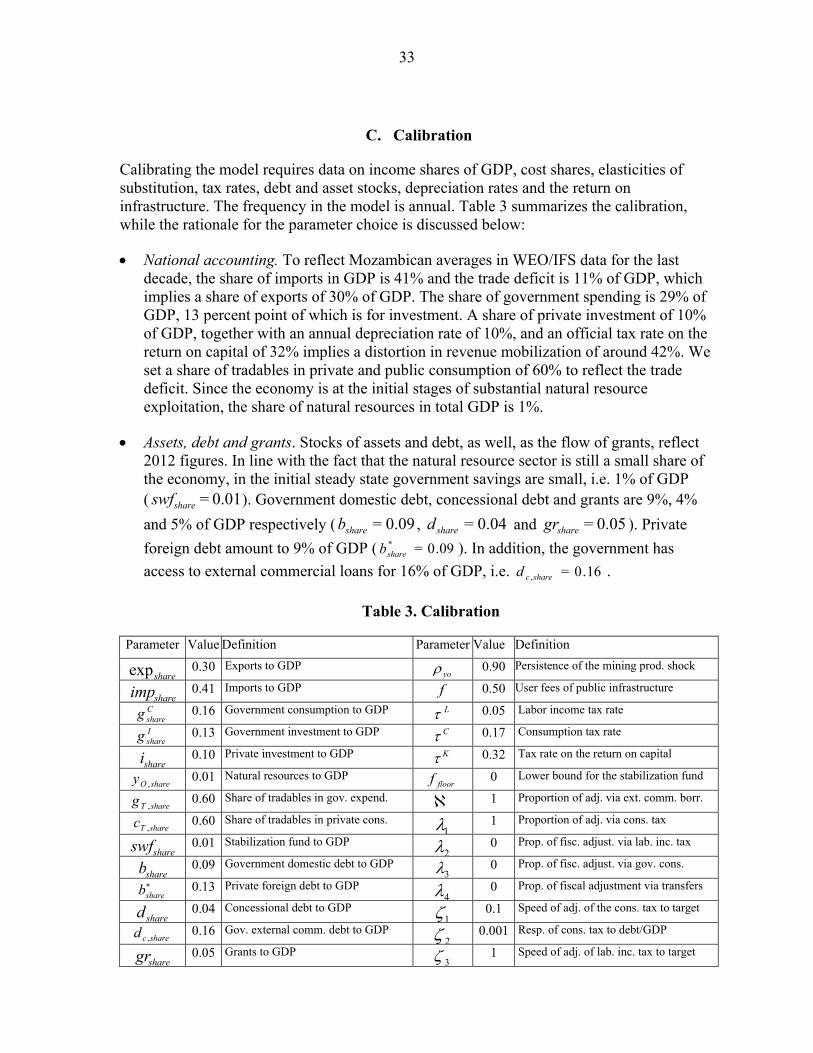
National accounting. To reflect Mozambican averages in WEO/IFS data for the last decade, the share of imports in GDP is 41% and the trade deficit is 11% of GDP, which implies a share of exports of 30% of GDP. The share of government spending is 29% of GDP, 13 percent point of which is for investment. A share of private investment of 10% of GDP, together with an annual depreciation rate of 10%, and an official tax rate on the return on capital of 32% implies a distortion in revenue mobilization of around 42%. We set a share of tradables in private and public consumption of 60% to reflect the trade deficit. Since the economy is at the initial stages of substantial natural resource exploitation, the share of natural resources in total GDP is 1%.

Assets, debt and grants. Stocks of assets and debt, as well, as the flow of grants, reflect 2012 figures. In line with the fact that the natural resource sector is still a small share of the economy, in the initial steady state government savings are small, i.e. 1% of GDP ( ). Government domestic debt, concessional debt and grants are 9%, 4%

and 5% of GDP respectively ( , and ). Private

foreign debt amount to 9% of GDP ( ). In addition, the government has

access to external commercial loans for 16% of GDP, i.e. .

Table 3. Calibration

Parameter Value Definition Parameter Value Definition

0.30 Exports to GDP 0.90 Persistence of the mining prod. shock

0.41 Imports to GDP 0.50 User fees of public infrastructure

0.16 Government consumption to GDP 0.05 Labor income tax rate

0.13 Government investment to GDP 0.17 Consumption tax rate

0.10 Private investment to GDP 0.32 Tax rate on the return on capital

0.01 Natural resources to GDP 0 Lower bound for the stabilization fund

0.60 Share of tradables in gov. expend. 1 Proportion of adj. via ext. comm. borr.

0.60 Share of tradables in private cons.

1 Proportion of adj. via cons. tax

0.01 Stabilization fund to GDP

0 Prop. of fisc. adjust. via lab. inc. tax

0.09 Government domestic debt to GDP 0 Prop. of fisc. adjust. via gov. cons.

0.13 Private foreign debt to GDP

0 Prop. of fiscal adjustment via transfers

0.04 Concessional debt to GDP

0.1 Speed of adj. of the cons. tax to target

0.16 Gov. external comm. debt to GDP

0.001 Resp. of cons. tax to debt/GDP

0.05 Grants to GDP 1 Speed of adj. of lab. inc. tax to target

0.01=shareswf

0.09=shareb 0.04=shared 0.05=sharegr

09.0=*shareb

16.0=,sharecd

shareexp yo

shareimp fCshareg LIshareg C

sharei KshareOy , floorf

shareTg , shareTc , 1shareswf 2

shareb 3shareb

4shared 1sharecd , 2sharegr 3

34

0.10 Domestic net real interest rate

0 Resp. of lab. inc. tax to debt/GDP

0.027 For. net real interest rate on savings

1 Speed of adj. of gov. spend. to target

0 Net real interest rate on conc. debt 0 Resp. of gov. cons. to debt/GDP

0.04 Net real risk-free rate

1 Speed of adj. of transfers to target

0.06 Net real int. rate on ext. comm. debt 0 Resp. of transfers to debt/GDP

0 Elasticity of sovereign risk

Floor on real government spending

0.45 Labor inc. share in non-traded sector Floor on real transfers

0.60 Labor income share in traded sector

Ceiling on consumption tax

0.10 Cap. deprec. rate in non-tradable sect.

Ceiling on labour income tax

0.10 Cap. depreciation rate in traded sector 0.6 Home bias of government purchases

0.10 Learning by doing in the traded sector 0.5 Home bias for add. government spending

0.10 Persistence in TFP in traded sector 0.25 Elast. of output to public capital

25 Invest. adj. cost in the non-traded sect. 0.07 Depreciation rate of public capital

25 Invest. adj. cost in the traded sector 0.60 Steady-state efficiency of pub invest.

10 Inv. of the Frisch elast. of labor supply 0.50 Planned long-term scaling up

2 Inv. of the inter-temp. elast. of subst.

- Speed of scaling up plan

1 Elast. of subst. betw. types of labor

- Degree of overshooting

0.60 Measure of optimizers in the economy 0.80 Pers. of depr. rate of public capital

0.44 Elast. of subst. betw. traded/non-traded 1 Severity of public capital depreciation

1 Elasticity of portfolio adiustment costs 20 Severity of absorp. capacity constraints

0.85 Royalty tax rate on natural resources

0.50 Thresholds of absorp. capac. constraints

1 Persist. of the commodity price shock

Interest rates. The coefficient of risk aversion, , set equal to 2 implies an inter-

temporal elasticity of substitution of 0.50 as common in the literature. We set the subjective discount rate, , such that the real net interest rate on domestic debt, , is 10%. Since the real interest rate on domestic debt and the real return on private capital are the same at the steady state, this is consistent with the estimated return on private capital in Dalgaard and Hansen (2005), but also with the stylized fact that domestic debt in low- and middle-income countries is usually more costly than external commercial debt.

In fact, we fix the real risk-free interest rate, at 4%, in line with average

historical real returns on US T-bill rates, and parameter such that the real interest rate

on external commercial debt, ), is 6%, in line with average IMF-World Bank

Debt Sustainability Analyses (IMF-WB DSAs). In addition, in IMF-WB DSAs, on average the real interest rate paid on concessional loans, , equal to 0%. No

additional risk-premium, , is assumed in the baseline calibration. Parameter is

chosen in order at the steady state, which is required by equations (A.7) and (A.8). Finally, based on average real returns of the Norwegian Government Pension Fund from

1R 4 1swfR 5 1dR 6 1fR 7 1,0 dcR

8dc C

floorg

N floorz

T Cceiling

N Lceiling

T

Ty g

Tz G

N G

T I

nssg

1k

2k

O GIpo

1)( R

1),( fR

dc1( dcR

1)( dR

0=dc u*= RR

35

1997 to 2011 (Gros and Mayer, 2012), the annual return on international financial assets is set equal to 2.7%.

Private production. In line with the evidence on Sub-Saharan Africa surveyed in Buffie et al. (2012), we set the labor shares of income in the non-traded and in the traded as

and , respectively. In both sectors private capital is assumed to

depreciate at an annual rate of 10% ( ). Following Berg et al. (2012) we

assume a minor degree of learning-by-doing externality in the traded sector ( ). Finally, following the calibration of Berg et al. (2010), investment

adjustment costs are set to .

Households preferences. Following Berg et al. (2012) a low Frisch labor elasticity of 0.10

( ) is assumed, in line with estimates of rural Malawi (Goldberg, 2011); the labor mobility parameter is set equal to unity (Horvarth, 2000), , and the elasticity of substitution between traded and non-traded goods is set equal to following Stockman and Tesar (1995). To capture the fact that the capital account has a low degree of openness, i.e. the private sector has limited access to international capital markets, we set as in Buffie et al. (2012). We set , which imply that 40% of consumers are entirely not savers.

Mining. Resource production shocks are assumed to be rather persistent, so we set

. This parameter is not relevant when a defined exogenous path for resource

production is assumed as we do in the simulations below. Given that Hamilton (2009) finds that oil prices follow a random walk with drift, and typically LNG is priced taking oil parity as a benchmark, we set . Finally the royalty tax rate, , is set such that

the ratio of natural resource revenue to total revenue at the peak of natural resource production is substantial, around 40% of total revenues. In this case

Tax rates. The steady-state taxes on consumption, and capital are , and

, respectively. We set the labor income tax rate at , lower than the official tax rates given that the model, featuring a representative agent, does not explicitely capture the fact many households do not pay income taxes in LICs. This combination of tax rates and the implied inefficiency in revenue mobilization imply a non-resource revenue of slightly above 20 percent of GDP at the initial steady state, which is broadly in line with Mozambican data.

Fiscal rules. We impose a non-negativity constraint for the stabilization fund by setting

. In our baseline calibration fiscal instruments do not have floors or ceilings.

0.45=N 0.60=T0.10== TN

0.10==TzTY

25== TN

10=1=

0.44=

1= 0.60=

0.90=yo

1=po O

0.85.=O

0.17=C0.32=K 0.05=L

0=floorf

36

This translates in setting and . The baseline

calibration also implies that the whole fiscal adjustment takes place through changes in external commercial borrowing and consumption taxes. This is achieved by setting

, , , . In addition, in order to

make tax changes smooth, we choose a small adjustment of the consumption tax rate to target of and a very low responsiveness of the consumption tax rate to the debt-

to-GDP ratio ( ).

Public investment. Public investment parameters broady follow the values chosen by

Berg et. al (2012) for the Angola and CEMAC region applications. In particular public investment efficiency is 60%, ( ), which is somewhat above the average LIC estimates of Gupta et al. (2011), to capture the fact that most infrastructure projects in Mozambique are planned to be executed by leading international companies. The depreciation rate for public capital is 7% per year ( ), somewhat lower than the depreciation rate of private capital given that the latter – in a model abstracting from durable goods – captures the depreciation of goods caracterized by a stronger degree of economic obsolescence. The home bias for public spending, , and for spending above the level of the initial steady state, , are 0.6 and 0.5, respectively. This captures the fact that, while at the steady state a bigger portion of public spending goes to the wages of public employees, in a public investment scaling up, much of the investment goods are imported in LICs. The elasticity of output to public capital is , which implies a marginal net return of public capital of 15% at the initial steady state. We normalize the severity of public capital depreciation to unity ( ) and make the depreciation rate of

public capital a persistent process ( ). We assume that absorptive capacity

constraints starts binding when public investment positively deviates beyond 50% from its initial steady state ( ), close to the estimates of Prichett (2000) for sub-

Saharan Africa and make of absorptive capacity constraints severe ( ) to an extent

that average investment efficiency approximately halves to around 30% if public investment were to spike to around 200% from its initial steady state. For illustrative purposes, in the delinked approach, we set the the planned long-term scaling up of investment such that public investment at the new steady state is 50% higher than at the initial steady state ( ). The speed of the scaling-up plan, , and the degree of

overshooting, , are chosen in different ways for alternative experiments and are reported in the following sections.

== floorCfloor zg == L

ceilingCceiling

1== 1 0=== 432 1=== 753 0=== 864

0.1=10.001=2

0.6=

0.07=G

g

0.25=G

1=0.8=

0.50=GI20=

0.50=Inssg 1k

2k