Surveying I.

Lecture 7.

Distance observations

Distance observations

• tapes;

• optical methods, e.g. using the stadia lines in the surveyor’s telescope;

• physical methods: electrooptical distance measurements (EDM)

Different ways to measure the distance between points:

Measuring distances with tapes

How long is a 30-meter-long tape?

Error sources:

• graduation error (1m on the tape is not equal to the standard 1 m);

• expansion caused by the pulling force;

• thermal expansion.

The effects must be taken into account to measure the distances accurately!

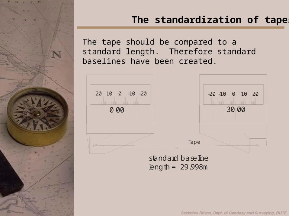
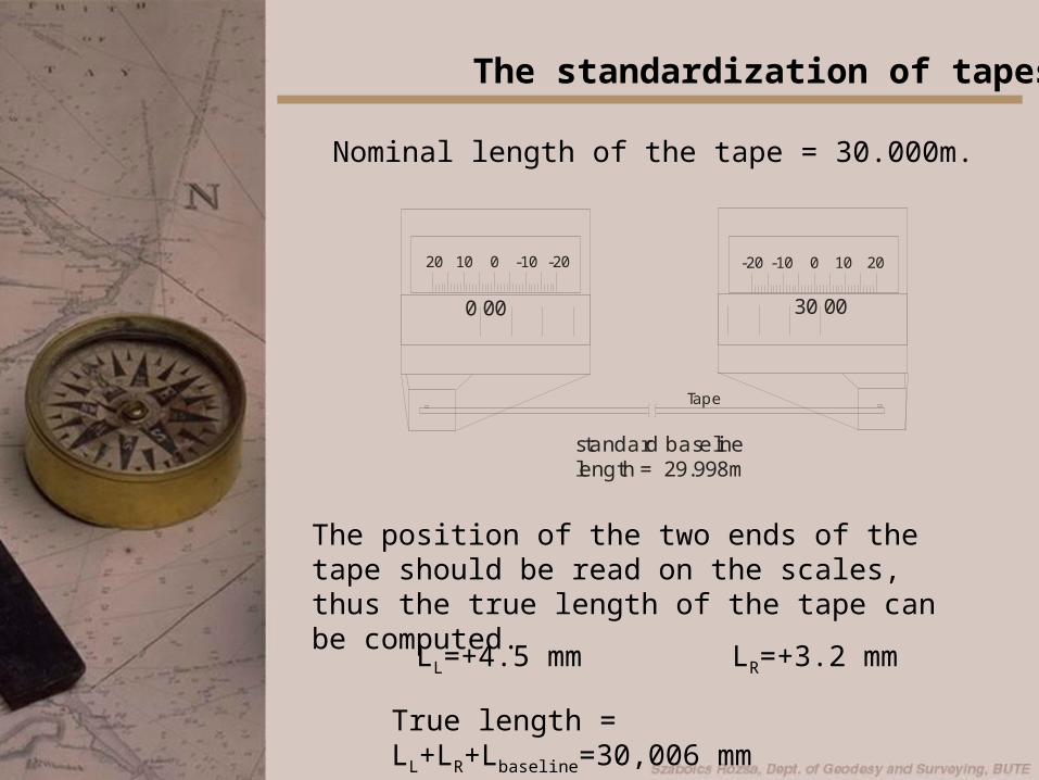
The standardization of tapes

The tape should be compared to a standard length. Therefore standard baselines have been created.

0 2010-10-200 -20-101020

0 00 30 00

standard baselinelength = 29.998m

Tape

The standardization of tapes

The position of the two ends of the tape should be read on the scales, thus the true length of the tape can be computed.

LL=+4.5 mm LR=+3.2 mm

True length = LL+LR+Lbaseline=30,006 mm

0 2010-10-200 -20-101020

0 00 30 00

standard baselinelength = 29.998m

Tape

Nominal length of the tape = 30.000m.

The standardization of tapes

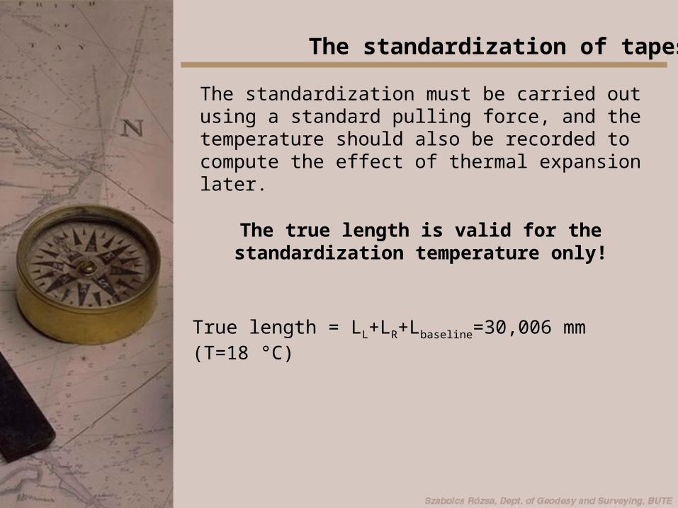
The standardization must be carried out using a standard pulling force, and the temperature should also be recorded to compute the effect of thermal expansion later.

The true length is valid for the standardization temperature only!

True length = LL+LR+Lbaseline=30,006 mm (T=18 °C)

The effect of pulling force and temperature

The effect of pulling force:

• when the same pulling force is used during the measurements as during the standardization, then the effect of this error source is eliminated.

The effect of temperature change:

• the temperature during the measurements must be recorded;

• the thermal expansion of the tape can be computed using the equation of thermal expansion of linear objects:

0TTLL

where is the expansion coefficient of the material of the tape (steel: =1.1x10-5 1/°C).

Physical Methods of Distance Observations

Indirect way of distance observation: the distance is measured by the observation of other physical variables.

Usually these methods are based on electromagnetic signals:• carrier signal – carries the measuring signal between the points; measuring signal – the carrier is modulated with this signal, and this is used for the distance observations

Two parts of the electromagnetic spectrum are used:• microwave (wavelengths are in the order of centimeters)• electrooptical (wavelengths are in the order of micrometers – visible light or infrared rays

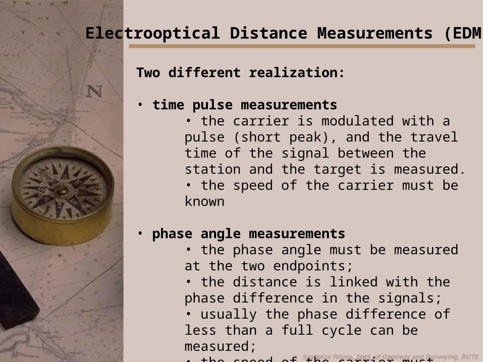
Electrooptical Distance Measurements (EDM)

Two different realization:

• time pulse measurements• the carrier is modulated with a pulse (short peak), and the travel time of the signal between the station and the target is measured.• the speed of the carrier must be known

• phase angle measurements• the phase angle must be measured at the two endpoints;• the distance is linked with the phase difference in the signals;• usually the phase difference of less than a full cycle can be measured;• the speed of the carrier must also be known;

The realization of EDM

A transmitter is place on the station, and a receiver on the target.

The carrier is modulated with the measurement signal, and transmitted by the instrument to the target.

The receiver receives the signal, demodulates it from the carrier, and uses the measurement signal to carry out the measurement.

Transmitter

Receiver

The realization of EDM

The distance can be computed using the phase difference or the travel time. However time synchronization is necessary to be able to measure these quantities.

We use a reflector at the target, and the receiver is placed in the instrument together with the transmitter:

TransmitterReceiver

Reflector

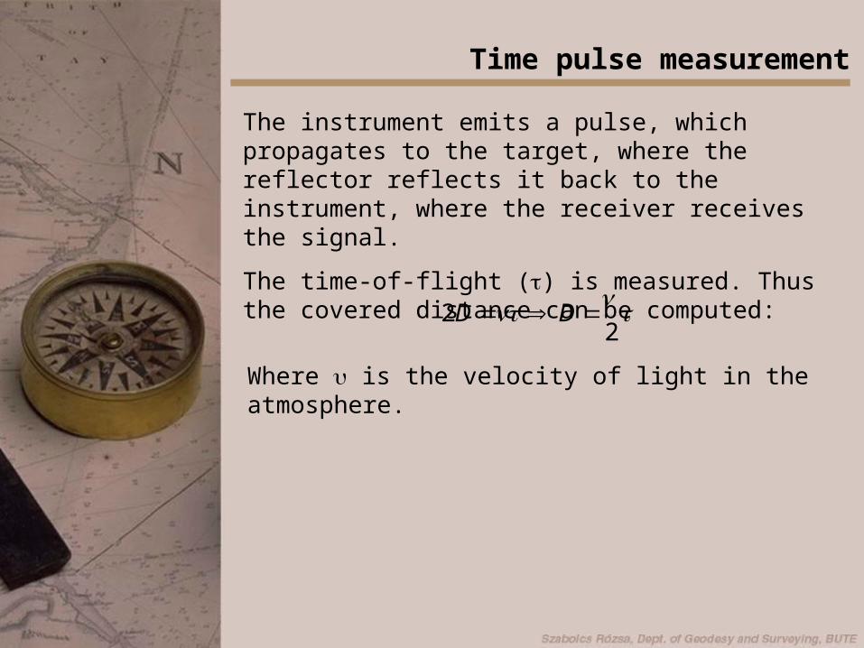
Time pulse measurement

The instrument emits a pulse, which propagates to the target, where the reflector reflects it back to the instrument, where the receiver receives the signal.

The time-of-flight () is measured. Thus the covered distance can be computed:

2

2 DD

Where is the velocity of light in the atmosphere.

Phase angle measurement

The signal travels the length of 2D.

Let’s suppose that and the frequency ( f ) of the measurement signal are known.

In this case the signal travels during a full cycle:

TransmitterReceiver

Reflector

f

Where is the wavelength of the signal.

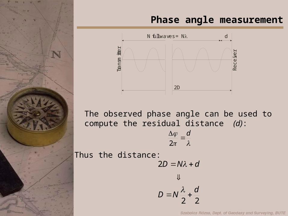
Phase angle measurement

2D

Trans

mitt

er

Receiv

er

N full waves = N d

d2

22

2

dND

dND

The observed phase angle can be used to compute the residual distance (d):

Thus the distance:

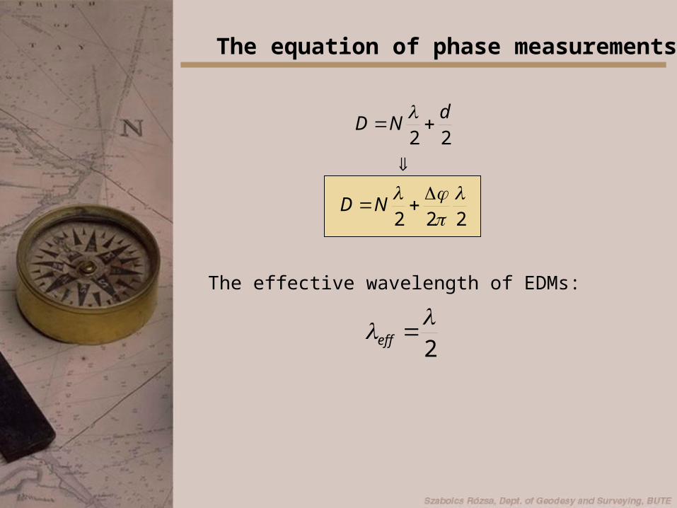
The equation of phase measurements

222

22

ND

dND

The effective wavelength of EDMs:

2 eff

The realization of phase measurements

222

ND

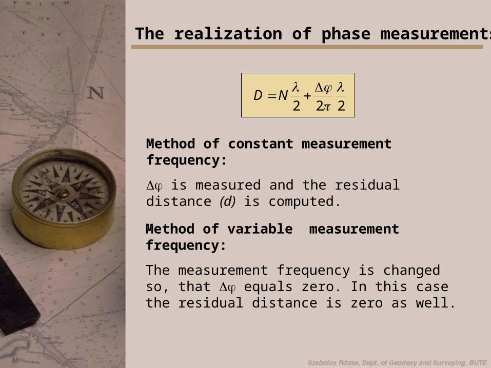
Method of constant measurement frequency:

is measured and the residual distance (d) is computed.

Method of variable measurement frequency:

The measurement frequency is changed so, that equals zero. In this case the residual distance is zero as well.

The determination of N

222

ND

When the effective wavelength is shorter than the observed distance, the observation is ambiguous (N is not known), but accurate.

When the effective wavelength is larger than the observed distance, the observation is unambiguous (N=0), but inaccurate due to the long wavelength.

The determination of N

2D

Trans

mitt

er

Receiv

er

N full waves = N2 2 d2

d1

N =01

Two different frequencies are used for the measurements:• 1 is larger than the range of the EDM• 2 provides the higher accuracy

2D

Trans

mitt

er

Receiv

er

N full waves = N2 2 d2

d1

N =01

The determination of N

The accuracy of phase angle measurement is usually 2-3/10000.

Let’s see the first observation (1eff=2000m):

N=0, accuracy is 0.6 md1 = 843.5 m

The determination of N

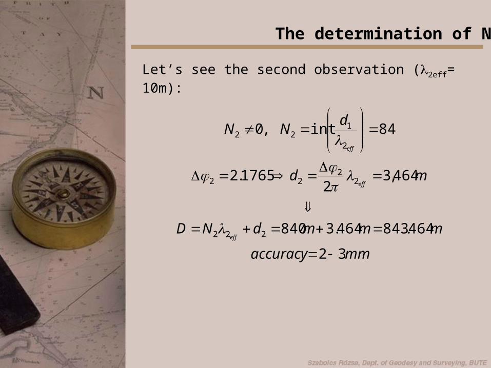
Let’s see the second observation (2eff= 10m):

mmaccuracy

mmmdND

md

dNN

eff

eff

eff

32

464.843464.3840

464,32

1765.2

84int,0

222

22

22

2

122

Error sources of EDMs

Instrumental and reflector constants

The transmitter is not aligned with the standing axis of the instrument, or the point of reflection is not aligned with the vertical of the target.

Instrumental offsets are automatically included in the results, but it is not the case with the prism offset.

Determining the reflector constant (c):Set out three collinear points (A,B and C), and measure the distances between AC in one set, and in two sets (AB and BC)!

The computation of the reflector constant

A B C

True distances: DAB, DAC, DBC

Observed distances: (D)AB, (D)AC, (D)BC

BCABAC

BCABAC

BCABAC

BCBCABABACAC

DDDc

cDcDcD

DDD

cDDcDDcDD

,

,

:since

Frequency error

Frequency error: the oscillators, which create the measurement signal are stable, but a drift can occur over a longer operational time.

A change in the frequency causes an error in the wavelength, thus in the observed distance as well.

222

ND

Instruments must be calibrated frequently, corrections can be applied to the observed distances (k).

rawDkD

fff

k

0

01

Atmospheric correction

f

The wavelength depends on the velocity of the signal in the atmosphere and the frequency.

The velocity of the signal depends on the refractive index of the atmosphere:

c

Where c is the velocity of light in vacuo, is refractive index.

The refractive index depends mostly on the air pressure and the temperature.

Atmospheric correction

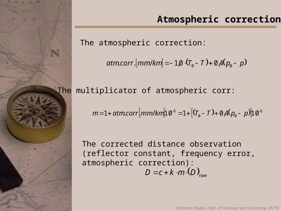
The atmospheric correction:

ppTTkmmmcorratm 00 4,00,1/..

600

6 104,0110/..1 ppTTkmmmcorratmm

The multiplicator of atmospheric corr:

The corrected distance observation (reflector constant, frequency error, atmospheric correction):

rawDmkcD

The reduction of distance observations

Definition: the distance between two points is defined by the distance between the two points projected to a reference surface (e.g. the Mean Sea Level).

Thus the measured distance should be reduced to this reference surface.

Note: Later we’ll see that the distances should also be reduced to the applied projection plane.

Reduction to the local horizon

The distance observations are usually measured on a slope. Therefore they should be converted to horizontal distances.

Slope distances can be:

• straight slopes,

• sections with different slopes.

Straight slope(e.g. EDM)

Sections with diff. slopes(e.g. tape)

Reduction to the local horizon

Sections with constant slopes can be converted to horizontal distances:

d

sh

A

B

If is known: d=s cos

if h is known: d=s-h2/2s.

Reduction to the Mean Sea Level

MSL

A’ B’

R

H

dAB

d’AB

O

H

dAB is the horizontal distance at the mean elevation ( ) of the two points

RH

ddd

HRR

dd

ABABAB

AB

AB

,

Thank You for Your Attention!