www.sciencemag.org/cgi/content/full/315/5820/1843/DC1

Supporting Online Material for

Emergent Biogeography of Microbial Communities in a Model Ocean

Michael J. Follows,* Stephanie Dutkiewicz, Scott Grant, Sallie W. Chisholm

*To whom correspondence should be addressed. E-mail: mick@mit.edu

Published 30 March 2007, Science 315, 1843 (2007)

DOI: 10.1126/science.1138544

This PDF file includes

Materials and Methods SOM Text Figs. S1 to S4 Table S1 References

- - 1

1

2

3

4 5 6 7 8 9

10

11

12

13

14

15

16

17

18

19

20

21

22

23 24 25 26 27 28 29 30 31 32

Supporting Online Material

METHODS:

S1. Ecosystem Model Algorithms.

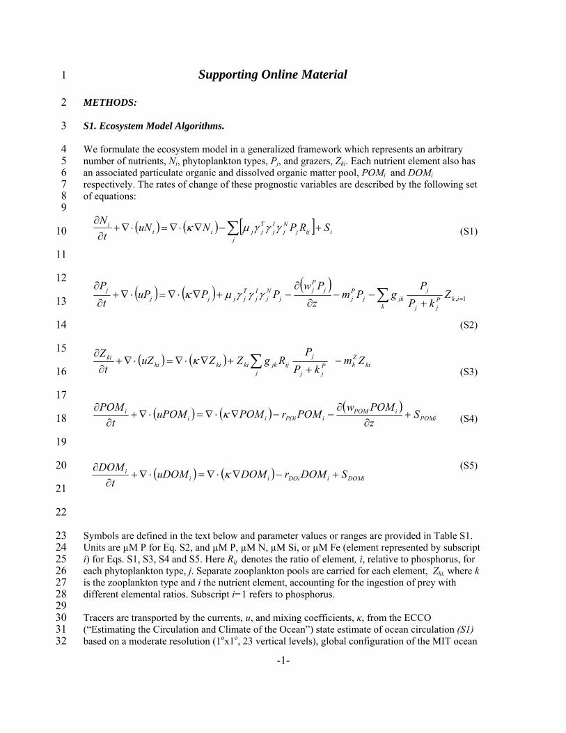
We formulate the ecosystem model in a generalized framework which represents an arbitrary number of nutrients, Ni, phytoplankton types, Pj, and grazers, Zki. Each nutrient element also has an associated particulate organic and dissolved organic matter pool, POMi and DOMi respectively. The rates of change of these prognostic variables are described by the following set of equations:

(S1) [( ) ( ) ] ij

ijjNIT

iii NuN

tN

+−∇⋅∇=⋅∂ ∑κ jjjj SRP∇+∂

γγγμ

( ) ( ) ( )

∑ =+−−

∂

∂−+∇⋅∇=⋅∇+

∂

∂

kikP

jj

jjkj

Pj

jPj

jNj

Ij

Tjjjj

j ZkP

PgPm

zPw

PPuPt

P1,γγγμκ

(S2)

(S3)

( ) ( ) ∑ −+∂ j

Pj

jk kP+∇⋅∇=⋅∇+

∂ki

Zk

j

jijkikiki

ki ZmP

RgZZuZt

Zκ

(S4) ( )( ) )(

(S5)

Symbols are defined in the text below and parameter values or ranges are provided in Table S1. Units are µM P for Eq. S2, and µM P, µM N, µM Si, or µM Fe (element represented by subscript i) for Eqs. S1, S3, S4 and S5. Here Rij denotes the ratio of element, i, relative to phosphorus, for each phytoplankton type, j. Separate zooplankton pools are carried for each element, Zki, where k is the zooplankton type and i the nutrient element, accounting for the ingestion of prey with different elemental ratios. Subscript i=1 refers to phosphorus. Tracers are transported by the currents, u, and mixing coefficients, κ, from the ECCO (“Estimating the Circulation and Climate of the Ocean”) state estimate of ocean circulation (S1) based on a moderate resolution (1ox1o, 23 vertical levels), global configuration of the MIT ocean

POMiiPOM

POiiii

zPOMwPOMrPOMuPOM

tPOM

i S+∂

∂−⋅∇+

∂−∇⋅∇=

∂ κ

( ) ( ) DOMiiDOiiii SDOMrDOMuDOM

tDOM

+−∇⋅∇=⋅∇+∂

∂ κ

- - 2

33 34 35 36 37 38 39 40 41 42 43 44

45

46

47 48 49 50

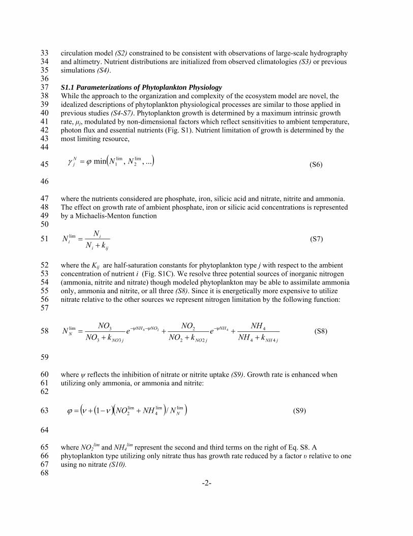
circulation model (S2) constrained to be consistent with observations of large-scale hydrography and altimetry. Nutrient distributions are initialized from observed climatologies (S3) or previous simulations (S4). S1.1 Parameterizations of Phytoplankton Physiology While the approach to the organization and complexity of the ecosystem model are novel, the idealized descriptions of phytoplankton physiological processes are similar to those applied in previous studies (S4-S7). Phytoplankton growth is determined by a maximum intrinsic growth rate, μj, modulated by non-dimensional factors which reflect sensitivities to ambient temperature, photon flux and essential nutrients (Fig. S1). Nutrient limitation of growth is determined by the most limiting resource,

(S6) ( )...,min Nj ϕγ = , lim2

lim1NN

where the nutrients considered are phosphate, iron, silicic acid and nitrate, nitrite and ammonia. The effect on growth rate of ambient phosphate, iron or silicic acid concentrations is represented by a Michaelis-Menton function

iji

ii kN

NN+

=lim (S7) 51

52 53 54 55 56 57

where the Kij are half-saturation constants for phytoplankton type j with respect to the ambient concentration of nutrient i (Fig. S1C). We resolve three potential sources of inorganic nitrogen (ammonia, nitrite and nitrate) though modeled phytoplankton may be able to assimilate ammonia only, ammonia and nitrite, or all three (S8). Since it is energetically more expensive to utilize nitrate relative to the other sources we represent nitrogen limitation by the following function:

jNH

NH

jNO

NONH

jNON kNH

NHekNO

NOekNO

NON44

4

22

2

33

3lim 424

++

++

+= −−− ψψψ (S8) 58

59

60 61 62

where ψ reflects the inhibition of nitrate or nitrite uptake (S9). Growth rate is enhanced when utilizing only ammonia, or ammonia and nitrite:

( )( )( )limlim4

lim2 /1 NNNHNO +−+= ννϕ (S9) 63

64

65 66 67 68

where NO2lim and NH4

lim represent the second and third terms on the right of Eq. S8. A phytoplankton type utilizing only nitrate thus has growth rate reduced by a factor υ relative to one using no nitrate (S10).

- - 3

69 70

Temperature modulation of growth is represented by a non-dimensional factor

( 2)(

1

01 ττ

γ −= −− CTTBTTj eA )71

72

73 74 75 76 77 78 79 80 81

(S10)

which sets a temperature range over which each phytoplankton type can grow efficiently (Fig. S1A), and there is a general decrease in growth efficiency with temperature (S11). Coefficients τ1 and τ2 normalize the maximum value, while A, B, To, and C regulate the form of the sensitivity envelope. We incorporate a very simple radiative transfer model (S4) which captures self-shading but does not resolve spectral bands. The light sensitivity of growth rate is parameterized using the function (S12):

( ) IkIkIj

inhibPAR eeF

−−−= 11

max

γ (S11) 82

83 84 85

where I(z) is the local, vertical flux of photosynthetically active radiation, PAR, and

⎟⎟⎠

⎞⎜⎜⎝

⎛⎟⎟⎠

⎞⎜⎜⎝

⎛+

−+

=inhibPAR

inhib

PAR

inhib

PAR

inhibPAR

kkk

kk

kkkF lnexpmax 86

87

88 89 90 91 92 93 94 95 96 97 98 99

100 101 102 103 104

is chosen to normalize the maximum value of to 1 (Fig. S1B). The parameter kIjγ par defines the

increase of growth rate with light at low levels of irradiation while kinhib regulates the rapidity of the decline of growth efficiency at high PAR, or photo-inhibition (S12). This highly idealized parameterization of light sensitivity captures variations in optimal light intensity, and their ecological implications, but does not explicitly account for photo-acclimation, differences in accessory pigments and other factors which might lead to variability in the maximum light dependent growth factor. We note that, while the function is normalized to a maximum value of 1 for all phytoplankton types, large size-class phytoplankton are given a higher maximum intrinsic growth rate, μ

Ijγ

j. We impose fixed elemental ratios for each phytoplankton type, Rij, though these may vary between types (e.g. some require silica while others do not). To restrict the niche dimension and computational expense of this initial study, we have imposed an average, Redfieldian N:P stoichiometry of 16:1 for all phytoplankton types. We note that in nature elemental ratios are flexible and Prochlorococcus, for example, can significantly exceed this value (S13). Formulating the model with dynamic nutrient quotas would capture flexible stoichiometry and is more physiologically appropriate (S14,S15) but also would significantly increase the number of three-

- - 4

105 106 107 108 109 110 111 112 113 114 115 116 117 118 119 120 121 122 123 124 125 126 127 128 129 130 131 132 133 134 135 136 137 138 139 140 141 142 143 144 145 146 147 148 149 150 151 152 153 154

dimensional arrays required to describe each phytoplankton type, dramatically increasing the computational expense. Hence we have not used this approach in this initial illustration. S1.2 Assignment of Physiological Functionality and Growth Rate Sensitivities. At the heart of this modeling strategy is the self-organization of a stochastically generated phytoplankton community. The physiological functionality and sensitivity of growth to temperature, light and ambient nutrient abundance for each modeled phytoplankton type is governed by several true/false parameters, the values of which are based on a virtual “coin-toss” at the initialization of each phytoplankton type. These determine the size class of each phytoplankton type (“large” or “small”), whether the organism can assimilate nitrate, whether the organism can assimilate nitrite, and whether the organism requires silicic acid. Parameter values which regulate the effect of temperature, light and nutrient availability on growth, are then assigned stochastically. To, which controls the optimum temperature for growth, and ΚPO4, the phosphate half-saturation coefficient (to which other half-saturations are indexed by the fixed elemental ratios), are drawn from prescribed ranges using a random number generator. Values for kpar and kinhib are also randomly chosen, drawn from prescribed normal distributions. Some simple allometric trade-offs are imposed (Fig. S1): Phytoplankton in the large size class are distinguished by higher intrinsic maximum growth rates and faster sinking speeds (S16). They also draw parameter values from distributions with higher nutrient half-saturations (assuming they are less efficient at acquiring nutrients, S17) and are assumed to be high-light adapted due to packaging effects (S18, S19). These trade-offs are implemented by randomly selecting parameter values from different (though overlapping) distributions for large and small phytoplankton. We note that, since the values of the governing coefficients are initialized stochastically from given distributions rather than prescribed specifically for each phytoplankton functional type, the total number of externally prescribed parameters in this approach (Table S1) is the same whether 10 or 10,000 phytoplankton types are initialized. The diversity of the “successful” population, and the parameter values that govern those organisms, are self-selected during the initial adjustment of the ecosystem model. S1.3 Grazing, Mortality, Remineralization and Biogeochemical Cycles. Parameterizations of grazing and other forms of heterotrophy are simplified in this study, which focuses on complexity and selection in the photo-autotrophs. None of the parameters regulating grazing and remineralization processes are stochastic in the simulations presented here. We prescribe a simple grazer community with two size classes. Large zooplankton preferentially graze (gfast) on large phytoplankton, but can graze on small phytoplankton (gslow) and visa versa for small zooplankton. A half-saturation coefficient (KP) regulates grazing efficiency at high prey concentrations. Excretion and non-grazing mortality are represented as linear loss terms for both phytoplankton and grazers, with coefficients mp and mz respectively. This simplified, low diversity grazer community is chosen to facilitate a computationally and intellectually tractable study in this initial illustration. Future studies should examine, for example, a greater diversity of grazers with a variety of stochastically appointed feeding strategies broadening the general strategy to include the next trophic level. The term Si (Eq. S1) represents the source of inorganic nutrient due to the remineralization of organic forms as well as external sources and non-biological transformations (S4,S17). Heterotrophic microbes are not explicitly represented and the remineralization of dissolved and particulate organic detritus pools is treated as a simple linear decay with respective prescribed timescales 1/rPOMi and 1/rDOMi (S4). SPOMi (Eq. S4) and SDOMi (Eq. S5) are the sources of particulate and dissolved organic detritus arising from mortality and excretion of all phytoplankton types and

- - 5

155 156 157 158 159 160 161 162 163 164 165 166 167 168 169 170 171 172 173 174 175 176 177 178 179 180 181 182 183 184 185 186 187 188 189 190 191 192 193 194 195 196 197 198 199 200 201 202 203

grazers (in Eq. S2 and S3), closing the nutrient budgets. Here we simply define a fixed fraction (fDOM) of mortality and excretion to pass into each organic detritus pool, assuming that large phytoplankton and zooplankton contribute a larger fraction of their detritus to the POMi pool than do the small phytoplankton. All silica is assumed to go to a POM pool, there is no dissolved organic silica. The remineralization of organic phosphorus and iron produce phosphate and dissolved iron respectively, while the remineralization of organic nitrogen is assumed to produce ammonia which may then be nitrified to nitrite and, subsequently, nitrate. The microbial process of nitrification is also treated simply as first order reactions with fixed rate coefficients (ζNO2, ζNO3) resulting in qualitatively reasonable distributions of the nitrogen species. Due to the relatively short timescale of the integrations and to restrict the complexity of this initial study we do not represent diazotrophy. Simplified one dimensional studies indicate that enabling diazotrophy as a possible functionality for the modeled phytoplankton types enhances the availability of more reduced forms of nitrogen in the subtropical regions resulting in an increase the abundance of Prochlorococcus analogs. Iron chemistry in seawater is parameterized (S20) with a complexation to an organic ligand (binding strength, βFe) and scavenging to falling particles (rate, cfe). Dust (S21) deposited in the surface (solubility, αfe) is a source of iron. SUPPORTING TEXT S2. Supplementary Model Results. An ensemble of model integrations was performed, each with a different randomization of physiological characteristics but identical initialization and physical environment. 78 phytoplankton types were initialized in each integration: Experimentation suggested that the modeled community structure would be less robust with fewer than 30, and practical computational considerations placed an upper limit at 78. Computational cost also limited the ensemble to only 10 members. Fig. S2 shows the annual mean concentration, at year 10, of phosphorus in biomass of the 78 phytoplankton from a single ensemble member. All ensemble members exhibit a similar set of occupied habitats which are collectively reminiscent of the previously proposed biogeographical provinces (S22). All ensemble members produce very similar total primary production and nutrient fields (shown for one member in Fig. S3), and these compare favorably to observations. The similarity in the total primary production reflects the significant regulation of physical nutrient supply and light on gyre and basin scales. The general biogeography of the model (depicted for a single ensemble member in Fig. 1B and Fig. S2) is robust between ensemble members. While various categorizations of “types” into functional groups might be considered, the classification here (Fig. 1B) reflects groupings of general interest and is tailored to reflect our particular interest in Prochlorococcus. . In general, the habitats of the emergent Prochlorococcus-analogs bear some qualitative resemblance to those observed but are much more sharply defined (Fig. 2, Fig. S4). Indeed, very low background abundances and sharply defined habitats of all the abundant, modeled phytoplankton types suggest that the model ecosystem is closer to complete competitive exclusion than is the real world (S23). This may reflect the relatively small number of

- - 6

204 205 206 207 208 209 210 211 212 213 214 215 216 217 218 219 220

physiological specializations (niche dimensions) in the model, the comparatively smooth, coarse resolution, physical environment (S24) or the low diversity of predatorial strategies (S23). Though each of the ten members of the ensemble of solutions are initialized with different randomization of the characteristics of the phytoplankton population, the emergent community structures and biogeography are relatively robust. For example, in each solution the four most abundant, emergent Prochlorococcus-analogs are relatively consistent (Fig. S3): the most abundant is typically of m-e1 classification and the second most abundant typically m-e2, with m-e3 type analogs at lower abundances. Although our model does not exhibit a significant deep (low light) biomass of Prochlorococcus-analogs (Fig. S4), there is a deep biomass maximum at the nutricline in the equatorial regions, comprised of “other small phytoplankton” types. Some of the phytoplankton types which make up this deep maximum might represent nitrate consuming Prochlorococcus strains which have been suggested from field observations (S25) but not yet cultured. Such organisms, though present in the model, are not classified as Prochlorococcus in our rather crude definition of functional groups.

- - 7

221 222 223 224 225 226 227 228 229

230 231 232 233 234 235 236 237 238 239 240 241 242 243 244 245

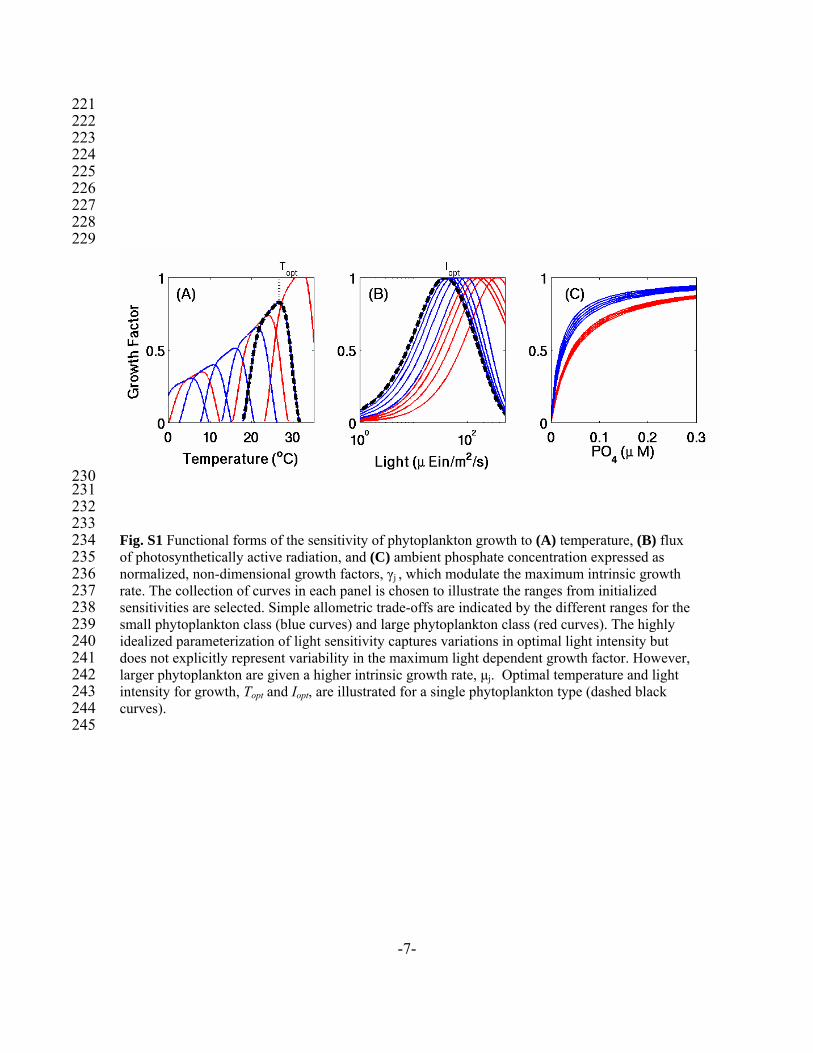
Fig. S1 Functional forms of the sensitivity of phytoplankton growth to (A) temperature, (B) flux of photosynthetically active radiation, and (C) ambient phosphate concentration expressed as normalized, non-dimensional growth factors, γj , which modulate the maximum intrinsic growth rate. The collection of curves in each panel is chosen to illustrate the ranges from initialized sensitivities are selected. Simple allometric trade-offs are indicated by the different ranges for the small phytoplankton class (blue curves) and large phytoplankton class (red curves). The highly idealized parameterization of light sensitivity captures variations in optimal light intensity but does not explicitly represent variability in the maximum light dependent growth factor. However, larger phytoplankton are given a higher intrinsic growth rate, μj. Optimal temperature and light intensity for growth, Topt and Iopt, are illustrated for a single phytoplankton type (dashed black curves).

246 247 248

Fig. S2. Phytoplankton abundance (μM P; average 0-50m, logarithmic color-scale) for each of 78 initialized types in a single ensemble member. Annual mean of tenth year of integration.

- - 8

249

250 251 252 253 254 255 256

Fig S3: Comparison of one ensemble member annual (0-50m) fields (right column) to observations (left column). (A,B) Primary Production (gC/m2/y); (C,D) Phosphate (µM P); (E,F) Nitrate (µM N); (G,H) Silicic Acid (µM Si). Observational euphotic layer primary production was calculated for 2005 using the Vertically Generalized Productivity Model (S26) and SeaWiFS-derived Chl. Data for this panel was downloaded from http://science.oregonstate.edu/ocean.productivity. Observational nutrients are from climatology of in situ data (S3) and are averaged over 0-50m.

- - 9

Fig. S4. The four most abundant Prochlorococcus-analogs (log(cells ml-1)) for the month of September along the AMT13 track from four of the ten member ensemble of integrations. “Type” number indicates the numerical designation of each of the 78 stochastically initialized phytoplankton types in each ensemble member. Analogs are classified into model-ecotypes as described in the main text. Model biomass is converted to cell density assuming a nominal phosphorus quota of 1 fg cell-1 for Prochlorococcus (13). Black contours are isotherms.

10

257 258 259 260 261

11

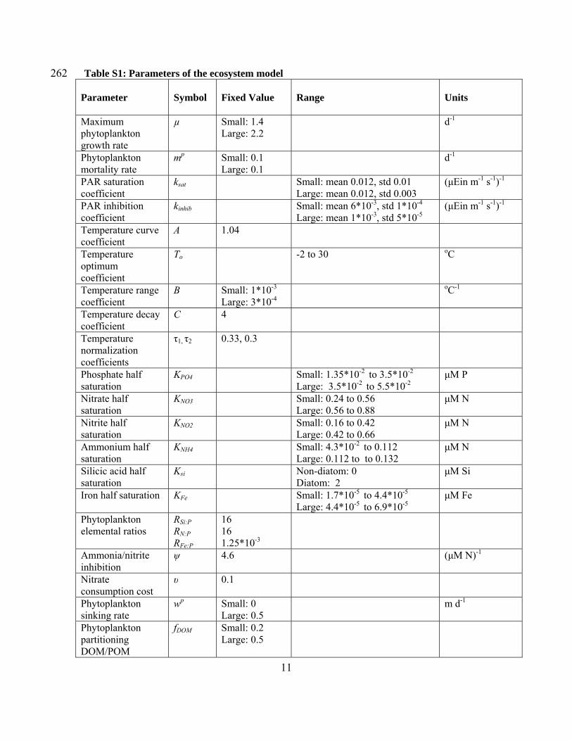
262 Table S1: Parameters of the ecosystem model Parameter

Symbol

Fixed Value

Range

Units

Maximum phytoplankton growth rate

µ

Small: 1.4 Large: 2.2

d-1

Phytoplankton mortality rate

mp Small: 0.1 Large: 0.1

d-1

PAR saturation coefficient

ksat Small: mean 0.012, std 0.01

Large: mean 0.012, std 0.003 (μEin m-1 s-1)-1

PAR inhibition coefficient

kinhib Small: mean 6*10-3, std 1*10-4

Large: mean 1*10-3, std 5*10-5(μEin m-1 s-1)-1

Temperature curve coefficient

A 1.04

Temperature optimum coefficient

To -2 to 30 oC

Temperature range coefficient

B Small: 1*10-3

Large: 3*10-4 oC-1

Temperature decay coefficient

C 4

Temperature normalization coefficients

τ1, τ2 0.33, 0.3

Phosphate half saturation

ΚPO4 Small: 1.35*10-2 to 3.5*10-2 Large: 3.5*10-2 to 5.5*10-2

μM P

Nitrate half saturation

ΚNO3 Small: 0.24 to 0.56 Large: 0.56 to 0.88

μM N

Nitrite half saturation

KNO2 Small: 0.16 to 0.42 Large: 0.42 to 0.66

μM N

Ammonium half saturation

KNH4 Small: 4.3*10-2 to 0.112 Large: 0.112 to to 0.132

μM N

Silicic acid half saturation

Ksi Non-diatom: 0 Diatom: 2

μM Si

Iron half saturation KFe Small: 1.7*10-5 to 4.4*10-5

Large: 4.4*10-5 to 6.9*10-5μM Fe

Phytoplankton elemental ratios

RSi:P RN:P RFe:P

16 16 1.25*10-3

Ammonia/nitrite inhibition

ψ 4.6 (μM N)-1

Nitrate consumption cost

υ 0.1

Phytoplankton sinking rate

wp Small: 0 Large: 0.5

m d-1

Phytoplankton partitioning DOM/POM

fDOM Small: 0.2 Large: 0.5

12

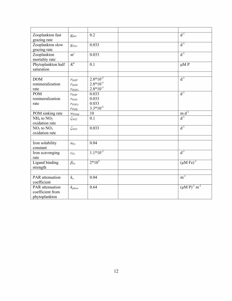
Zooplankton fast grazing rate

gfast 0.2

d-1

Zooplankton slow grazing rate

gslow 0.033 d-1

Zooplankton mortality rate

mz 0.033 d-1

Phytoplankton half saturation

Kp 0.1 μM P

DOM remineralization rate

rDOP rDON rDOFe

2.8*10-3

2.8*10-3

2.8*10-3

d-1

POM remineralization rate

rPOP rPON rPOFe rPOSi

0.033 0.033 0.033 3.3*10-3

d-1

POM sinking rate wPOM 10 m d-1

NH4 to NO2 oxidation rate

ζNO2 0.1 d-1

NO2 to NO3 oxidation rate

ζNO3 0.033 d-1

Iron solubility constant

αFe 0.04

Iron scavenging rate

cFe 1.1*10-3 d-1

Ligand binding strength

βFe 2*105 (μM Fe)-1

PAR attenuation coefficient

ko 0.04 m-1

PAR attenuation coefficient from phytoplankton

kphyto 0.64 (μM P)-1 m-1

13

263 264 265 266 267 268 269 270 271 272 273 274 275 276 277 278 279 280 281 282 283 284 285 286 287 288 289 290 291 292 293 294 295 296 297 298 299

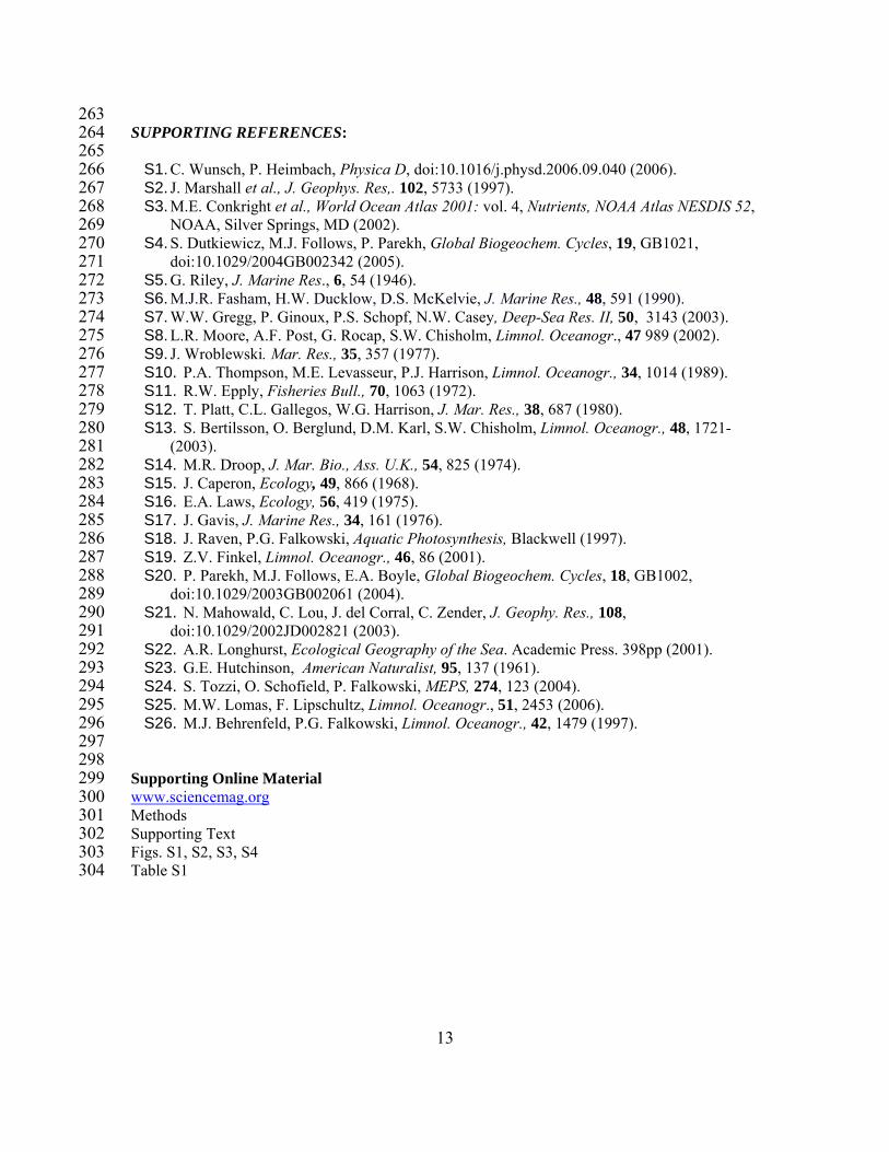
SUPPORTING REFERENCES:

S1. C. Wunsch, P. Heimbach, Physica D, doi:10.1016/j.physd.2006.09.040 (2006). S2. J. Marshall et al., J. Geophys. Res,. 102, 5733 (1997). S3. M.E. Conkright et al., World Ocean Atlas 2001: vol. 4, Nutrients, NOAA Atlas NESDIS 52,

NOAA, Silver Springs, MD (2002). S4. S. Dutkiewicz, M.J. Follows, P. Parekh, Global Biogeochem. Cycles, 19, GB1021,

doi:10.1029/2004GB002342 (2005). S5. G. Riley, J. Marine Res., 6, 54 (1946). S6. M.J.R. Fasham, H.W. Ducklow, D.S. McKelvie, J. Marine Res., 48, 591 (1990). S7. W.W. Gregg, P. Ginoux, P.S. Schopf, N.W. Casey, Deep-Sea Res. II, 50, 3143 (2003). S8. L.R. Moore, A.F. Post, G. Rocap, S.W. Chisholm, Limnol. Oceanogr., 47 989 (2002). S9. J. Wroblewski. Mar. Res., 35, 357 (1977). S10. P.A. Thompson, M.E. Levasseur, P.J. Harrison, Limnol. Oceanogr., 34, 1014 (1989). S11. R.W. Epply, Fisheries Bull., 70, 1063 (1972). S12. T. Platt, C.L. Gallegos, W.G. Harrison, J. Mar. Res., 38, 687 (1980). S13. S. Bertilsson, O. Berglund, D.M. Karl, S.W. Chisholm, Limnol. Oceanogr., 48, 1721-

(2003). S14. M.R. Droop, J. Mar. Bio., Ass. U.K., 54, 825 (1974). S15. J. Caperon, Ecology, 49, 866 (1968). S16. E.A. Laws, Ecology, 56, 419 (1975). S17. J. Gavis, J. Marine Res., 34, 161 (1976). S18. J. Raven, P.G. Falkowski, Aquatic Photosynthesis, Blackwell (1997). S19. Z.V. Finkel, Limnol. Oceanogr., 46, 86 (2001). S20. P. Parekh, M.J. Follows, E.A. Boyle, Global Biogeochem. Cycles, 18, GB1002,

doi:10.1029/2003GB002061 (2004). S21. N. Mahowald, C. Lou, J. del Corral, C. Zender, J. Geophy. Res., 108,

doi:10.1029/2002JD002821 (2003). S22. A.R. Longhurst, Ecological Geography of the Sea. Academic Press. 398pp (2001). S23. G.E. Hutchinson, American Naturalist, 95, 137 (1961). S24. S. Tozzi, O. Schofield, P. Falkowski, MEPS, 274, 123 (2004). S25. M.W. Lomas, F. Lipschultz, Limnol. Oceanogr., 51, 2453 (2006). S26. M.J. Behrenfeld, P.G. Falkowski, Limnol. Oceanogr., 42, 1479 (1997).

Supporting Online Material www.sciencemag.org300

301 302 303 304

Methods Supporting Text Figs. S1, S2, S3, S4 Table S1