Bank substitutability and financial

network resilience: insights from the

first globalization

Abstract:

The recent literature on financial network resilience has paid relatively less attention to the

dimension of substitutability than to interconnectedness. In this paper, we apply a simple technique to simulate the upper-bound effects of bank defaults on firms’ access to credit at the

global level during the first globalization (1880-1914). We find that, in stark contrast to today’s

financial networks, in the early 20th century the global network displayed considerable resilience to shocks, as the level of substitutability of all banks was relatively high. This finding

has implications for regulators, as it shows that a financial network not featuring highly-

systemic banks can (and did) actually exist.

Keywords: money market; bill of exchange; financial network resilience; substitutability; chain-

based methodology

JEL codes: B40, E42, G23, L14, N20

This work, co-authored with Olivier Accominotti (London School of Economics and CEPR)

and Stefano Ugolini (Sciences Po Toulouse), is from Chapter 5 of Delio Lucena-Piquero’s PhD

dissertation: “Beyond the Dyadic Approach in Social Network Analysis: Applications to

Innovation Studies and Financial Economics” (2020). The London School of Economics has

kindly provided the financial support for the collection of the data used in this work.

1

1. Introduction

Since the 2008 crisis, academics and policymakers have been deeply concerned with the

question of the identification of systemic actors in financial systems. Traditionally, regulators

had been mostly identifying systemic intermediaries according to their size (the “too-big-to-fail

approach”), but the catastrophic effects generated by the fall of Lehman Brothers (a relatively

small bank) brought to light the multidimensional nature of systemicness. In 2013, the Basel

Committee on Banking Supervision (BCBS) and the Financial Stability Board (FSB) jointly

published new guidelines for the assessment of systemicness, based on five different dimensions

of the concept: size, interconnectedness, substitutability, complexity, and cross-jurisdictional

activity (BCBS, 2013).1 Among these five dimensions, interconnectedness is the one that has

attracted larger academic attention in the last decade or so: many scholars have been applying

network analysis and simulation techniques in order to identify “too-interconnected-to-fail”

actors, thus reaching a number of important conclusions about the structural properties and

resilience of modern financial networks. By contrast, substitutability has attracted relatively less

attention to date. Assessing substitutability has however proved particularly problematic (Benoit

et al., 2019), leading regulators to revise their guidelines under this respect (BCBS, 2018).

In this paper, we use simple network analysis and simulation techniques in order to assess more

specifically the relationship between actors’ substitutability and financial network resilience.

Our approach is straightforward: we provide an upper-bound evaluation of network disruption

due to financial shocks by looking at how many actors remain isolated once intermediaries are

removed. This is an upper-bound estimation as it rests on the (very strong) assumption that no

other financial relationship can exist except those that are actually observed – meaning that an

agent will lose market access if the intermediaries to which she is connected do default.

Applying this methodology to contemporary financial networks yields very catastrophic results:

networks break down as central nodes are removed, thus pointing to the high degree of

unsubstitutability of a few actors (see e.g. Pröpper et al., 2008). This result might be taken as a

confirmation of the conclusion (a general one for studies based on contemporary data) that

financial networks inevitably feature a few highly systemic actors. However, in this paper we

apply this methodology to an historical financial network and we reach very different

conclusions: in our case study, node removal never generates sizable damage in the network,

1 Size is defined as the total size of the bank’s liabilities. Interconnectedness consists of the network of contractual

obligations that characterize the bank’s activities. Substitutability (sometimes referred to as “financial institution

infrastructure”) is defined as the bank’s importance as a provider of client services. Complexity consists of the

business, structural, and operational complexity of the bank (i.e., its involvement in sophisticated activities such as

derivatives or other off-balance-sheet exposures). Cross-jurisdictional activity is the geographical dispersion of the

bank’s activities (BCBS, 2013).

2

thus pointing to low levels of systemicness for all actors. Note that our case study does not

consist of an idiosyncratic, peripheral financial market from an obscure historical epoch, but no

less than the global money market at the heyday of the first globalization (1880-1914), when the

international economy reached levels of interconnectedness comparable to those of the late 20th

century (O’Rourke and Williamson, 2002). We are therefore able to provide, for the first time,

evidence that a financial network featuring can exist and did actually exist globally at a time of

high international integration. In our view, this finding yields potentially important implications

for regulators.

The rest of the paper is organized as follows. Section 2 reviews the recent literature applying

network analysis and simulation techniques, and highlights the originality of our paper. Section

3 describes our data and details our empirical strategy. Section 4 presents our results. Section 5

concludes and offers some speculations for regulators.

2. Literature review

2.1. Financial stability and network analysis: introduction

The 2008 crisis has proved that the failure of relatively small but highly interconnected

intermediaries can lead to a large-scale breakdown of the financial system, generating huge

economic and social costs. As a result, the study of the topology of financial systems,

mobilizing network analysis techniques, has gained considerable momentum in recent years.

The “macroprudential” network perspective questions the traditional “microprudential”

assumption that the financial system is safe as long as each individual intermediary is safe, and

highlights the importance of relational structures as a driving factor of the robustness of the

system. The pioneering work of Allen and Gale (2000) has been the first to underline the role of

the topology of the financial network, and more concretely its connectivity, on default

contagion. Another founding block of this literature is the work of Freixas et al. (2000), who

focused on the structural importance that some individual actors may acquire, and urged

regulators to switch from the traditional “too-big-to-fail” approach to a “too-connected-to-fail”

approach. Since then, the number of studies taking a network perspective has increased,

addressing both the effect of network structure on the dynamics and resilience of the financial

systems and the processes of network formation (Allen and Babus, 2009). Useful surveys of this

substantial research effort include Glasserman and Young (2016), Battiston and Martinez-

Jaramillo (2018), Caccioli et al. (2018), and Iori and Mantegna (2018).

3

In this section, we do not aim to provide an exhaustive summary of this literature, but only to

focus on the aspects that are more relevant from the perspective. The first one is the question of

the availability of information about financial interlinkages – an issue that has “daunted” a large

part of the research that has been conducted so far. The second one has to do with the typologies

of network structures that the literature has been finding (or generating) while dealing with

financial networks. The third aspect we focus on is the way in which shocks are simulated in

order to test the resilience of network structures. Last (but not least), we look at the

interconnection between financial and non-financial networks, in order to see how the

transmission of financial shocks to the real economy has been tackled by the literature.

2.2. Data availability

The issue of the nature and treatment of data has been seldom addressed from a critical

perspective. Most financial markets, especially interbank markets, are characterized by a high

degree of opacity concerning the distribution and size of financial exposures (Espinosa-Vega

and Solé, 2010; Upper, 2011; Blasques et al., 2015). As a natural strategy, researchers have

often chosen to make estimations of the exchanges when primary data were not available,

inferring bilateral credit relationships from balance sheet or payments data (Furfine, 1999;

Upper and Worms, 2004; Allen and Babus, 2009; Upper, 2011). It is through this practice that it

has been possible to reconstruct the structure of the interbank networks of e.g. Switzerland

(Sheldon and Maurer, 1998), Austria (Boss et al., 2004), Belgium (Degryse and Nguyen, 2004),

Germany (Upper and Worms, 2004), the UK (Wetherilt et al., 2010), or the US (Bech and

Atalay, 2010).

Since the quality of an analysis depends on the quality of its data, these estimation practices

have been criticized (Upper, 2011). Some comparative analyses have pointed to some serious

problems in using estimated data. For instance, after comparing simulated and actual data on the

Italian interbank network, Mistrulli (2011) concluded that simulations may overstate contagion.

More recently, Anand et al. (2018) performed a ‘horse race’ between different methods for

reconstructing complete interbank networks from incomplete datasets, only to conclude that no

optimal method does actually exist. As a result, while relatively rare, original databases on

actual network structures are naturally superior and potentially more insightful (Iori and

Mantegna, 2018, pp. 651-3). This justifies the wealth of research that has been conducted on the

Italian interbank network, which is the only one for which complete transaction data are actually

available (see e.g. Iori et al., 2008; Fricke and Lux, 2015a, 2015b; Iori et al., 2015; Temizsoy et

al., 2015).

4

Another important limitation of many of the researches in this literature is the fact that the

nature of the databases they rely on is actually strictly national. Papers taking an international

perspective only look at country-country linkages rather than individual linkages (Espinosa-

Vega and Solé, 2010; Minoiu and Reyes, 2013; Chinazzi et al., 2013; Minoiu et al., 2015). One

exception is the research conducted on syndicated loan networks (Hale et al., 2016; Cai et al.,

2018), but this is based on data from a rather “niche” market whose representativeness of the

broader interbank network remains unclear. As a result, to the best of our knowledge, no

database on the global financial network has been available to researchers to date.

2.3. Network structures

Reconstructing the structural properties of financial networks is key in order to assess their

resilience to shocks and its implications for policymakers. One very relevant property is the

presence of a core-periphery structure, which can be measured through several indicators as the

degree distribution2 or the level of disassortativity.3 The idea is to identify if there exists a small

group of highly-connected actors centralizing flows and thus playing the role of “hubs”. This

has important implications in terms of the vulnerability of the network to shocks. As much as in

the general literature on networks (e.g. Albert et al., 2000; Newman, 2003), in the financial

literature core-periphery structures present a high degree of robustness to random shocks to

individual actors, but they become extremely fragile when shocks involve actors playing the

role of hubs – a situation known as the “robust-yet-fragile” tendency (Gai and Kapadia, 2010).

Empirical studies on modern financial networks generally found core-periphery structures (in

some cases referred as scale-free structures)4 with high levels of disassortativity (Craig and Von

Peter, 2014). This is the case of domestic interbank networks e.g. in Austria (Boss et al., 2004),

Germany (Upper and Worms, 2004), Switzerland (Müller, 2006), the UK (Wetherilt et al.,

2010), or the US (Soramäki et al., 2007). Analyses of the global country-to-country financial

network (Minoiu and Reyes, 2013; Chinazzi et al., 2013) equally found evidence of core-

periphery, disassortative networks. In the words of Fricke and Lux (2015b, p. 391), “a similar

hierarchical structure […] might be classified as a new ‘stylized fact’ of modern interbank

networks”.

2 The hierarchy refers to the distribution of the nodes’ degree in a network, and a network is hierarchical if a small

number of actors are significantly higher than most actors in the network. 3 The assortativity is a measure of similarity usually based on node degree correlation, and a network is assortative if

nodes with high/low degree are connected to actors with also high/low degree. 4 In theory, core-periphery and scale-free structures are not the same thing. In practice, however, it is difficult to

discriminate between the two in empirical investigations. The reasons why this is the case are explained by Iori and

Mantegna (2018, p. 645).

5

Only a minority of empirical studies found evidence of less hierarchical structures, featuring a

weaker core-periphery structure and lower levels of disassortativity. This was viz. the case for

domestic interbank networks in Italy (Iori et al., 2008; Fricke and Lux, 2015a), the Netherlands

(Blasques et al., 2015), and Mexico (Martinez-Jaramillo et al., 2014). These findings have led

some authors to criticize the use of scale-free models in the reconstruction of network structures

from partial data (Martinez-Jaramillo et al., 2014; Fricke and Lux, 2015a; Anand et al., 2018).

2.4. Shock simulations

The network approach is a useful way to represent contagion due to externalities, but different

types of mechanisms can generate financial contagion: these include defaults, distress that is not

conducive to default, the common structure of assets, or the common structure of liabilities

(Battiston and Martinez-Jaramillo, 2018, pp. 7-8). As the concern of our paper is with market

access, we limit our review to the question of defaults. As a matter of fact, this is the issue that

has been vastly dominating the literature on financial network resilience. Since the pioneering

work of Allen and Gale (2000), several papers have applied shock simulation techniques

(sometimes drawn from epidemiologic models) in order to understand if and how “epidemies”

(cascades) of defaults might develop in financial networks (see esp. Gai and Kapadia, 2010).

Two main approaches to the modelling of default cascades can be found in the literature. The

most common one has been initiated by the seminal paper of Eisenberg and Noe (2001), who

modelled default cascades in the payment network as a function of interbank exposures: every

node suffers a shock from its incoming links and spreads it proportionally through its outcoming

links. Eisenberg and Noe’s (2001) “fictitious default algorithm” has been used and developed

by a number of scholars (including e.g. Müller, 2006; Battiston et al., 2012a, 2012b; Acemoglu

et al., 2015; Glasserman and Young, 2015) in order to simulate “domino effects” in the

interbank market. This methodology yields several advantages, but it also has some drawbacks.

The first one is that it requires very restrictive assumptions on the way contagion spreads across

the network: the behaviour of each node is necessarily mechanical, which casts doubts on its

usefulness for policy guidance (Allen and Babus, 2009; Upper, 2011). The second drawback is

that this methodology is very much demanding in terms of information, as it requires complete

interbank exposures to be known. As such information is often unavailable, however, the

precondition to its application is that complete interbank exposures are reconstructed from

partial data through some estimation techniques (see above), which raises doubts on its

adequacy to represent real-world shocks.

6

An alternative (and much simpler) methodology consists of merely suppressing defaulting

nodes, and thus measuring the damage that such suppressions generate to the network’s

connectivity. This methodology is quite popular in network analysis (see e.g. Albert et al., 2000;

Newman, 2003; Cohen and Havlin, 2010; Li et al., 2015), although less so in the study of

financial networks (one example is Pröpper et al., 2008). It is obviously less sophisticated than

the Eisenberg-Noe approach, but it has the clear advantage of being much less demanding in

terms of information, as it only requires the general structure of the network (and not the weight

of each link) to be known. In our study, we opt for this simpler methodology, which appears to

be more suited for studies focused on the concept of market access and actor substitutability.

2.5. Bank-firm networks

The overwhelming share of the network-based literature on financial contagion has focused on

interactions between financial intermediaries (bank-bank networks). Only a handful of papers

have managed to go beyond this limitation, by adding to bank-bank links also bank-firm links.

As a matter of fact, bank-firm relationships are essential to understanding the transmission of

financial contagion to the real economy, but the availability data on such relationships has been

very limited to date. The few cases for which information has been made available include

Japan (De Masi et al., 2011), Italy (De Masi and Gallegati, 2012), and Brazil (Silva et al.,

2018). The “stylized facts” retrieved from such empirical investigations have inspired the model

of Lux (2016), which allows simulating the spillovers of financial contagion from bank-bank to

bank-firm relationships.

One common feature of all these papers is the fact of representing bank-bank and bank-firm

links as two different layers of the same multiplex network. This kind of representation has a

number of advantages, yet the analysis of interactions between the different layers of multiplex

financial networks still remains in its infancy (Battiston and Martinez-Jaramillo, 2018, pp. 11-3;

Iori and Mantegna, 2018, pp. 647-8). Moreover, representing bank-bank and bank-firm

relationships as de facto two different (albeit interconnected) networks may obfuscate the

gatekeeping role often played by financial actors. As a matter of fact, banks lending to firms are

most often used to refinancing themselves from other banks, thus only playing the role of

“bridges” between the borrower and the ultimate lender. In such a case, the “bridging” function

implemented by gatekeepers is lost in this kind of representation (on this point, also see

Bonacich et al., 2004). As we want to focus specifically on this function, we therefore opt not to

represent our data through a multiplex network, but rather through a hypergraph (see below,

7

Section 3.2). To our knowledge, we are the first ones to do so in the literature on financial

contagion.

2.6. Literature review: summary

Our review of the network-based literature on financial contagion allows drawing a number of

considerations. a) The crucial role of network structures in determining the path and extent of

financial contagion is now universally acknowledged for contemporary financial systems. b)

This notwithstanding, only limited information on the complete structure of financial networks

is available to date, and scholars have been forced to reconstruct such structures through

estimation techniques that present some inconveniences; moreover, most papers have had to

take a strictly national perspective, as very limited information exist on global financial

networks. c) Based on the above-mentioned reconstructions, most papers have tended conclude

that financial networks inevitably assume hierarchical core-periphery structures characterized

by a high level of disassortativity; only a minority of papers have nuanced (albeit only partially)

this very stark view. d) Simulations of “default cascades” have mostly been based on a number

of restrictive assumptions, which may limit their ability to represent real-world crises. e) Only a

handful of papers have been concerned with the transmission of financial contagion from bank-

bank to bank-firm relationships; in all cases, the two types of relationships have been

represented as different layers of a multiplex network, yet this does not allow appreciating the

“bridging” role (between borrowing firms and lending banks) actually played by some banks.

Our paper is therefore original under many respects. a) To the best of our knowledge, this is the

first paper to investigate the role of network structures in financial contagion from an historical

perspective. b) It is based on observed data on actual financial connectivity rather than on

estimated data; moreover, it features data on the global financial network rather than national

data. c) In contrast to the findings of the literature on contemporary systems, we evidence the

existence of a financial network with a rather weak core-periphery structure and low levels of

disassortativity. d) Finally, our data features information not only on bank-bank relationships,

but also on bank-firm relationships; moreover, we are the first to focus specifically on the

gatekeeping role of banks by representing bank-bank-firm relationships as continuous chains

(see below, Section 3.2).

8

3. Empirical strategy

3.1. Data

Our empirical analysis is based on an original database of global financial interlinkages at the

time of the first globalization (1880-1914). In those times, London was the unrivalled global

financial centre and the sterling-denominated bill of exchange was the staple international

money market instrument (Accominotti and Ugolini, forthcoming). Painstakingly hand-

collected from archival sources, our dataset includes information on 23,493 bills of exchange

issued on the sterling money market during the calendar year 1906. A detailed discussion on the

nature and representativeness of these data can be found in our historical companion paper

(Accominotti et al., 2021).

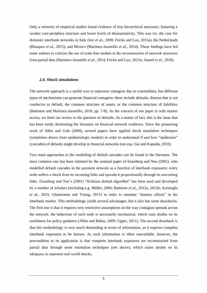
As illustrated by Figure 1, the origination and distribution of a bill of exchange always involved

at least three fundamental actors: one borrower (the “drawer”, a firm), one guarantor (the

“acceptor”, an intermediary), and one lender (the “discounter”, generally a bank or a money

market fund). As our archival source provides systematic information on all three roles for each

bill, we are therefore able to track all borrower-guarantor (“firm-bank”) and guarantor-lender

(“bank-bank”) relationships: this allows us drawing the complete network of interlinkages for

the core global money market of the time. We end up with a static network of 4,970 nodes: of

these, only 1,680 (33.80%) were located in London, while the rest was spread throughout the

five continents (Accominotti et al., 2021).

3.2. Chains

As said (see above, Section 2.5), all of the papers studying the effects of financial contagion on

the real sector have treated firm-bank and bank-bank relationships as two different layers of a

Firm-Bank Relationship

Drawer

(Borrower)

Acceptor

(Guarantor)

Discounter

(Lender)

Bank-Bank Relationship

Figure 1: The origination and distribution chain of a bill of exchange 1

9

multiplex network. In this paper, we make a different choice. In order to keep the unity of the

borrower-guarantor-lender relationship, we treat each bill as a three-unit chain or triad (drawer-

acceptor-discounter), which is a hyperedge of a hypergraph (forming a hyperstructure)5.

(Criado et al., 2010). More formally, within a population of individuals V, a bill is a chain Ci

defined as a non-empty set (i, j, k) ∊ V where it exists a borrower-guarantor relationship ( iTj )

and a guarantor-lender relationship ( jUk )6: so Ci =(iTjUk) ∀ {i, j, k} ∈ V ∧ {T, U} ∈ R.

Additionally, we define a network of chains as a hypergraph H=(V, E) / ∀ Ci ∃ Ei, or in other

words, every chain Ci corresponds to an edge or hyperedge Ei. Representing chains as

hyperedges of a hypergraph (forming a hyperstructure) allows preserving the unity and

configuration of the chains. Additionally, hypergraphs provide a flexible analytical framework

that allows using simple social network measures that cannot be applied to multilayer networks

without further adjustments, as e.g. several types of degree centrality (see below).

We are not the first ones to use hypergraphs as a way to preserve supra-dyadic structures.

Bonacich et al. (2004), Estrada and Rodríguez-Velázquez (2006), and Battiston et al. (2020) all

stressed that traditional dyadic-based graphs do not provide a complete description of complex

real-world systems, and recommended the use of hypergraphs to study “higher-order” (i.e.,

supra-dyadic) systems. However, common hypergraph approaches (including the ones

mobilized in the three above-mentioned works) do not allow preserving the internal

configuration of supra-dyadic structures, because they do not reproduce the links existing

between individuals and the positions occupied by nodes within such structures. This problem

can be solved through the introduction of hyperstructures, as suggested by Criado et al. (2010).

To illustrate their intuition, these authors give the example of a subway network. This network

is composed by the subway stations (the nodes) and the trunks between them (the links).

Stations and trunks are grouped as subway lines, which can be considered as substructures of

the subway network. Two stations may be separated by the same number of trunks, but a

traveller moving between the two will face quite a different situation if the stations are on the

same line or not. In order to take this into account, it is convenient to consider the whole

subway network as a hypergraph and the single subway line as hyperedges. Then, the

hyperstructure will consist of the combination of an adjacency matrix (representing all the

stations and the trunks between them) and a hypergraph (where each hyperedge is a subway

line, grouping all its stations and branches). Criado et al. (2010) only considered hyperstructures

5 A hypergraph is a generalization of a graph in which an edge (called hyperedge) groups one or several nodes, and

every node is related to a hyperedge. A hyperstructure is an association between an adjacent matrix – which indicates

every dyadic link between nodes – and a hypergraph – which groups one or several nodes of the adjacent matrix by

hyperedges. Thus, a hyperstructure is a hypergraph which includes every dyadic link between nodes. 6 Note that nodes’ specialization is not absolute: in theory, each actor can play all three roles. In our data, however,

“hybrid” nodes are relatively rare (see below, Section 4.2).

10

with symmetric (non-oriented) relations. Our contributions extend their original intuition by

considering hyperstructures with directed (oriented) relations.

3.3. Shock simulations in chains

In order to test the resilience of the resulting financial network to shocks, we opt for simple

node removal simulations (see above, Section 2.4). Specifically, we alternatively simulate the

removal of individual upstream nodes (guarantors or lenders, i.e. the nodes situated in position 2

or 3 of each chain), and we examine the impact of the suppression in terms of loss of market

access for downstream nodes (borrowers and guarantors, i.e. the nodes situated in position 1 or

2 of each chain).7 Thus, the structural relevance of each removed node is measured as the

number of downstream actors who are strictly dependent on it in order to obtain market access

(i.e, to be connected to an upstream actor). A downstream actor is considered as independent if

it is connected to other nodes providing it with access market (i.e., if it has other paths to reach

an upstream actor). The number of downstream actors losing market access in case of the

removal of an upstream actor is thus taken as the indicator of the degree of substitutability of the

latter.

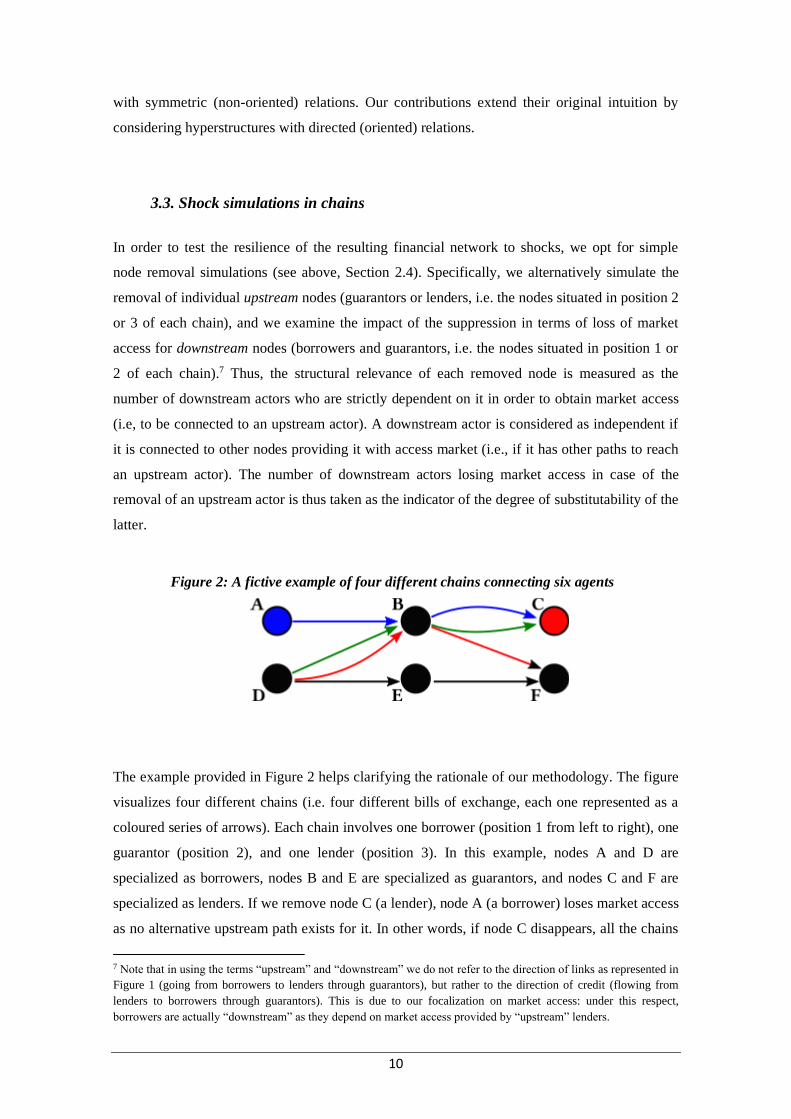
Figure 2: A fictive example of four different chains connecting six agents 2

The example provided in Figure 2 helps clarifying the rationale of our methodology. The figure

visualizes four different chains (i.e. four different bills of exchange, each one represented as a

coloured series of arrows). Each chain involves one borrower (position 1 from left to right), one

guarantor (position 2), and one lender (position 3). In this example, nodes A and D are

specialized as borrowers, nodes B and E are specialized as guarantors, and nodes C and F are

specialized as lenders. If we remove node C (a lender), node A (a borrower) loses market access

as no alternative upstream path exists for it. In other words, if node C disappears, all the chains

7 Note that in using the terms “upstream” and “downstream” we do not refer to the direction of links as represented in

Figure 1 (going from borrowers to lenders through guarantors), but rather to the direction of credit (flowing from

lenders to borrowers through guarantors). This is due to our focalization on market access: under this respect,

borrowers are actually “downstream” as they depend on market access provided by “upstream” lenders.

11

in which it is involved (blue and green arrows) also disappears, and this includes the link

between A and B, thus making borrower A isolated. By contrast, the suppression of lender C

has no impact on market access for borrower D, as the latter is linked to another lender (i.e.

node F) via a compound relationship through guarantor E (represented by the red arrows).

Notice that if we had implemented a traditional node removal without paying attention to the

compound nature of the relationship, the suppression of lender C would have had no impact on

the connectivity of borrower A. This, however, would have been oblivious of the reality of

market access: as a matter of fact, in reality lender F is unwilling to lend to borrower A, and this

path is therefore actually unavailable to A. This underlines the importance of preserving the

integrity of actual chains while simulating shocks.

Concretely, we proceed as follows. In our network defined by the hypergraph H=(V, E) / ∀ Ci ∃

Ei of chains Ci = (i,j,k) defined by (iTj ∪ jUk), consider an element x ∈ (jUk) (i.e., an upstream

actor, acceptor or discounter). Any element y ∈ Ci ∧ y ≠ x has an alternative access to the

market if ∃ Cj : x ∉ Cj ∧ y ∈ Cj. On other words, we first identify all the chains in which the

given element plays the upstream role of acceptor or discounter (we call it the reference set for

this element), and we single out all the other actors involved in these chains. Then we check if

each of the individual downstream actors of the reference set is present in any other of the

chains in our dataset. If an actor is already present in at least one other chain, we consider it as

having an alternative market access: thus, the node is not strictly dependent on the upstream

element, as it does not get isolated when the latter disappears. To the contrary, if the actor is not

present in any other chain, we consider it as not having any alternative market access: thus, the

node is strictly dependent on the upstream element, as it gets isolated when the latter disappears.

4. Results

4.1. Results: Introduction

In order to test our network’s resilience to individual defaults, we proceed as follows. In Section

4.2, we provide some descriptive statistics on the network and its structure. In Section 4.3, we

first apply the methodology described above (Section 3.3) and measure the absolute impact of

the suppression of individual nodes – viz., the number of nodes that remain isolated following

the default of each intermediary. We find that the systemic damage generated by the

suppression of individual nodes is always relatively limited, which points to a low degree of

unsubstitutability for all nodes. This is our baseline result. In the subsequent sections, we

perform a number of robustness checks.

12

In Section 4.4, we ask whether some nodes might have displayed some “local” systemicness: to

tackle this question, we measure the relative impact of the suppression of individual nodes –

viz., the share of the total downstream nodes that remain isolated. We find that some nodes did

display some local unsubstitutability, yet this was mainly the case for nodes with low rather

than high absolute impact.

In Section 4.5, we measure the “group” systemicness of some (exogenously-defined) groups of

intermediaries that are recognized to have played an extremely relevant role in the global

financial system. We find that, even in the most catastrophic scenarios (in which an entire

segment of the financial sector defaults), our network does not break down completely – which

points to relatively low levels of unsubstitutability even for crucial segments of the financial

sector.

In Section 4.6, we ask whether some nodes might have displayed some “geographic”

systemicness – viz., if their removal would leave some geographic locations cut off from the

global financial network. We find that some nodes did display some local unsubstitutability, yet

this was mainly the case for nodes with low rather than high absolute impact.

Finally, in Section 4.7 we measure the degree of vulnerability of geographic locations

throughout the world to the default of financial intermediaries in London. We find that on

average most cities displayed a relatively limited level of vulnerability, and that such a level was

insensitive to city size.

Therefore, all robustness checks are consistent with our baseline result, suggesting that the

early-20th-century global financial network displayed a high degree of resilience to individual

defaults and was not prone to the “robust-yet-fragile” tendency.

4.2. Descriptive statistics

In this section we provide some descriptive statistics concerning the population of our network,

and present its macro structure by comparing its degree distribution to simulated both random

and free-scale degree distributions.

As explained above (see Figure 1), each chain is formed by the sequence of the three roles,

where acceptors and discounters may be located only in London, while drawers may be located

anywhere in the world (including London). While most individuals are specialized in one role,

some take several roles (we call them “hybrids”). Table 1 shows the distribution of individuals

13

by role and location, as well as the proportion they represent with respect to the total population

and to the population of actors located in London.

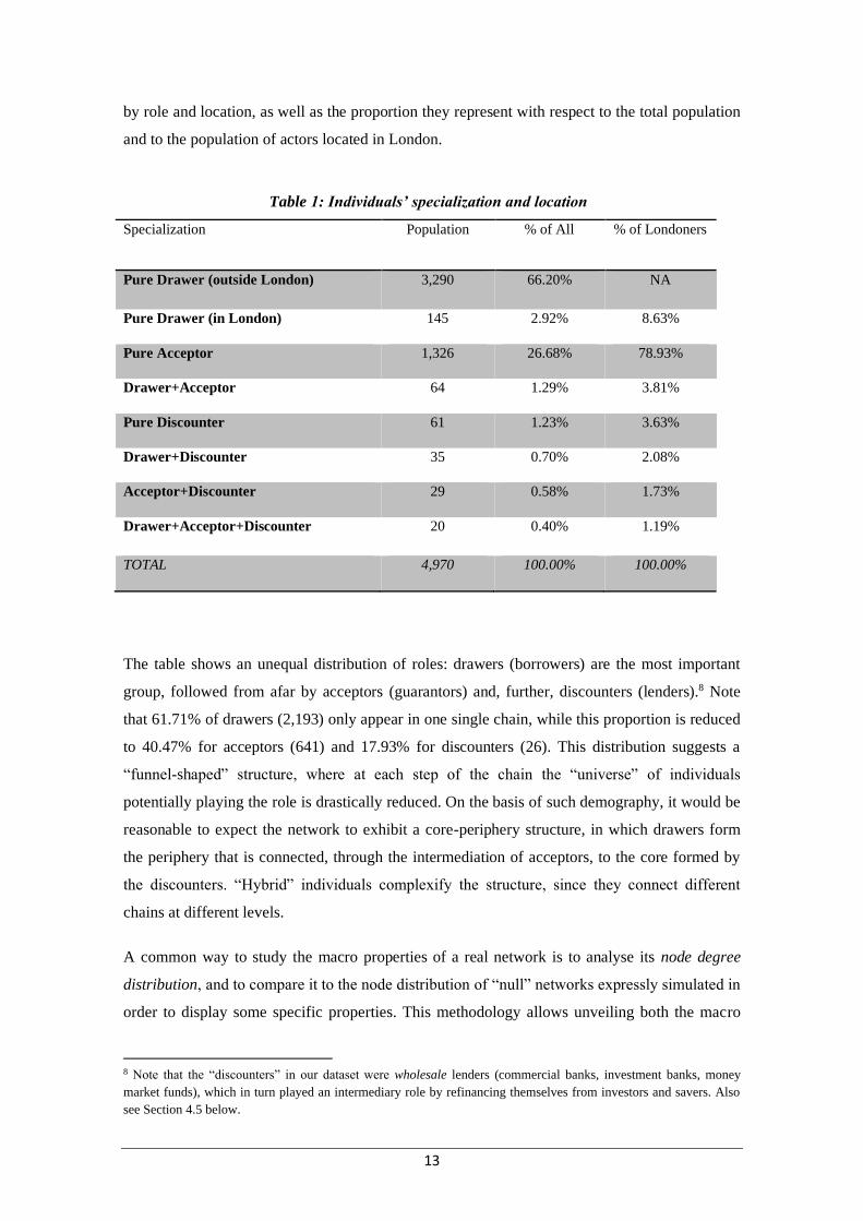
Table 1: Individuals’ specialization and location 1

Specialization Population % of All % of Londoners

Pure Drawer (outside London) 3,290 66.20% NA

Pure Drawer (in London) 145 2.92% 8.63%

Pure Acceptor 1,326 26.68% 78.93%

Drawer+Acceptor 64 1.29% 3.81%

Pure Discounter 61 1.23% 3.63%

Drawer+Discounter 35 0.70% 2.08%

Acceptor+Discounter 29 0.58% 1.73%

Drawer+Acceptor+Discounter 20 0.40% 1.19%

TOTAL 4,970 100.00% 100.00%

The table shows an unequal distribution of roles: drawers (borrowers) are the most important

group, followed from afar by acceptors (guarantors) and, further, discounters (lenders).8 Note

that 61.71% of drawers (2,193) only appear in one single chain, while this proportion is reduced

to 40.47% for acceptors (641) and 17.93% for discounters (26). This distribution suggests a

“funnel-shaped” structure, where at each step of the chain the “universe” of individuals

potentially playing the role is drastically reduced. On the basis of such demography, it would be

reasonable to expect the network to exhibit a core-periphery structure, in which drawers form

the periphery that is connected, through the intermediation of acceptors, to the core formed by

the discounters. “Hybrid” individuals complexify the structure, since they connect different

chains at different levels.

A common way to study the macro properties of a real network is to analyse its node degree

distribution, and to compare it to the node distribution of “null” networks expressly simulated in

order to display some specific properties. This methodology allows unveiling both the macro

8 Note that the “discounters” in our dataset were wholesale lenders (commercial banks, investment banks, money

market funds), which in turn played an intermediary role by refinancing themselves from investors and savers. Also

see Section 4.5 below.

14

structure of the real network and the relational dynamics that drive its link creation (e.g. Craig

and Von Peter, 2014; Martinez-Jaramillo et al., 2014). We follow this standard procedure and

compare the node degree distribution of our observed network to the degree distribution of 100

simulated random (Erdös-Renyi) networks and 100 simulated scale-free networks displaying the

same demography of the observed ones. On the one hand, because in random networks any two

individuals have the same probability to be linked to each other, simulated random networks are

used as baselines (e.g. Iori et al., 2015; Chinazzi et al., 2013) in order to unveil the existence of

any relational dynamics (i.e. any kind of biases) guiding link creation and the formation of the

macro structure of the network. On the other hand, simulated scale-free networks are used as

baseline in order to unveil the existence of one specific relational dynamic – viz., the

preferential attachment dynamics, which is conducive to core-periphery macro structures (e.g.

Martinez-Jaramillo et al., 2014; Iori and Mantegna, 2018). Following the preferential

attachment principle, individuals tend to connect preferentially to well-connected actors rather

than to poorly-connected ones: this generates core-periphery structures, where most of the

population connect to a small group of well-connected individuals. As said above (Section 2c),

empirical investigations have mostly found core-periphery structures in modern interbank

systems.

Hypergraphs allow for great flexibility in the definition of network measures, including the

node degree (Battiston et al., 2020; Kapoor et al., 2013). In order to properly describe the macro

structure of our network, we use three different definitions of node degree: 1) the node’s in-

degree, defined as the number of its adjacent nodes linked by an input-arc; 2) the node’s

hyperedge degree, defined as the number of node’s incident hyperedges – i.e., the number of

hyperedges (in our case, chains) in which an individual is involved; and 3) the node’s

hyperedge’s adjacent nodes degree, defined as the number of nodes that belong to the same

hyperedge (chain).

To build the simulated networks, we keep the original drawers-bills distribution (i.e., we

consider that the bills’ origin does not change, so each drawer preserves its original number of

bills) as well as the original number of individuals in the acceptor and discounter roles.

Consequently, simulated networks preserve the same demography and number of chains of the

observed network.

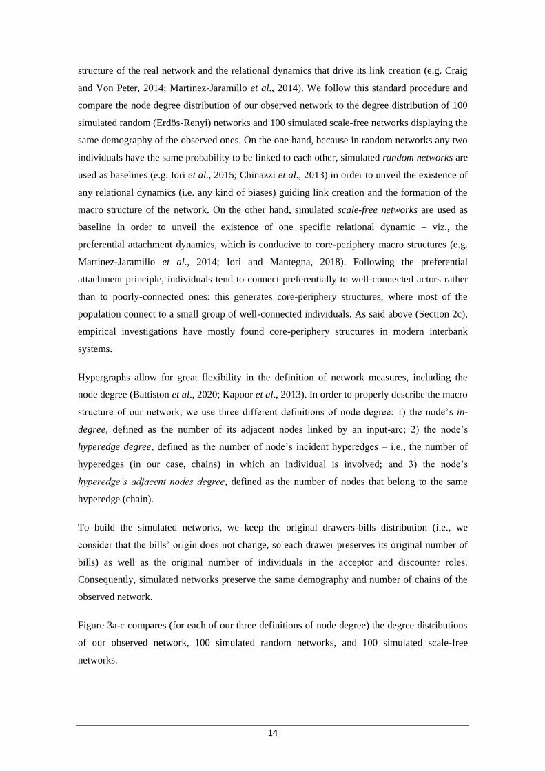
Figure 3a-c compares (for each of our three definitions of node degree) the degree distributions

of our observed network, 100 simulated random networks, and 100 simulated scale-free

networks.

15

Figure 3: Degrees distributions of observed and simulated networks 3

For each of our three definitions of degree (see text), the figures show the degree distribution of our

observed network (black lines), of 100 simulated random networks (blue lines), and of 100 simulated

scale-free networks (lines). The x axes represent the degree value through a natural logarithmic scale. The

y axes correspond to the percent of individuals sharing the same degree value. Vertical lines (in blue,

black, and red) represent the highest degree value for (respectively) random, observed, and scale-free

networks. Since all drawers have in-degree 0, they have been removed from Figure 3a.

Three features emerge from Figure 3a-c. First, the degree distributions of our observed network

are very different from those of random networks, which highlights the presence of some kind

of relational dynamics in link creation. Second, the degree distributions of the observed network

are more similar to, yet still somewhat different from those of free-scale networks. Third,

16

regarding the highest degree for each type of distribution (vertical lines), the ones of the

observed network is situated between those of random and those of free-scale networks. These

elements suggest that, although there do exist some relational dynamics determining the link

creation behaviour, these dynamics do not perfectly follow a preferential-attachment rule, which

would be conducive to a core-periphery macro structure.

Some interesting features emerge from a more detailed observation. Hyperedges’ adjacent nodes

degree distributions exhibit irregular shapes (peaks), esp. in simulated networks (see Figure 3c).

The first peak is formed by the first three degree values and is common to all types of networks.

The first value (corresponding to degree 1) represents an atypical situation in which an

individual is involved in chains (usually, one single bill) that include only one other individual –

i.e., the chain has one individual appearing twice in two different roles. This is due to the

existence of “hybrid” individuals intervening at different steps of the same chain.9 The presence

of this type of behaviour is higher (2.11% of individuals) in the observed network since some

intentionality, and not only a statistical probability, is required for this kind of combination to

occur. The degree value 2 (top of the peak) is very common (57.56% of individuals in the

observed network), and represents a situation where the individual is involved in one or several

chains with two other individuals. This situation is typical for drawers, especially those involved

in one only transaction. Higher degree values necessarily require the individual to be involved

in several chains. The situation where several chains link the individual to three other ones

(degree 3) is very unusual in the simulated networks but not in the observed network. This is

also the case for higher degree values.

To sum up, the demography of our network would, a first sight, suggest the existence a core-

periphery macro structure (as modern interbank networks). Although at this stage we cannot

completely reject the “null” hypothesis that link formation in our network is dictated by a

preferential attachment rule, the presence of very highly interconnected nodes (represented by

the highest degree values) is much lower in our observed network than in simulated free-scale

networks with the same demography. This suggests that the sort of “mega-hubs” found in

present-day interbank networks did not exist in the early-20th-century global financial network.

In what follows, we will address this question more specifically.

9 In our data, this situation occurs in case the same individual plays at the same time the role of drawer (borrower)

and discounter (lender) of the same bill. This apparent paradox is due to the fact that discounters were wholesale

lenders, and used bills as collateral for refinancing their operations with retail lenders: in some cases, some

discounters “created” bills in order to refinance themselves under the guarantee of an acceptor (Accominotti et al.,

2021).

17

4.3. Absolute systemicness

As explained in Section 3.3, our methodology assumes that removal from the network of one

individual implies that the operations (bills) in which it is involved cannot be performed, and

the impact of this removal is measured by the number of individuals who strictly depend on

those very chains for their market access. As said, this is an upper bound estimate of the degree

of unsubstitutability of upstream actors, as it rests on the assumption that downstream actors

will not have any chance to connect to any other upstream actor – which is a very restrictive

assumption indeed. Thus, in order to assess the absolute systemicness of individuals, we remove

them one by one from the network, we identify the chains that are impacted, and we count how

many individuals are left isolated. We only focus on the absolute systemicness of individuals

playing the upstream role of acceptor (guarantor) and/or discounter (lender), which means a

total of 1,535 individuals. We do not consider individuals playing the role of drawers

(borrowers): since they are located in the beginning of chains, their systemicness is by

construction equal to zero.

For each individual i, we compute: (a) the Acceptor Impact AImpi, which is the number of

individuals who remain isolated when the individual i is removed from her acceptor role; (b) the

Discounter Impact DImpi, which is the number of individuals who remain isolated when the

individual i is removed from her discounter role; (c) the Total Impact TImpi, which is the

number of individuals who remain isolated when the individual i is removed from her

acceptor/discounter role; (d) the Total Impact Rate TImpRi = (TImpi / (n-1))*100, which is

percent of all actors n of the network who remain isolated when the individual i is removed; and

(e) the Market Share MSi = (ni / (n-1) )*100, which is the share of all the actors in the network

(n) who are involved in the same chains as individual i (ni).

18

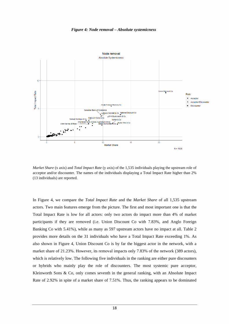
Figure 4: Node removal – Absolute systemicness 4

Market Share (x axis) and Total Impact Rate (y axis) of the 1,535 individuals playing the upstream role of

acceptor and/or discounter. The names of the individuals displaying a Total Impact Rate higher than 2%

(13 individuals) are reported.

In Figure 4, we compare the Total Impact Rate and the Market Share of all 1,535 upstream

actors. Two main features emerge from the picture. The first and most important one is that the

Total Impact Rate is low for all actors: only two actors do impact more than 4% of market

participants if they are removed (i.e. Union Discount Co with 7.83%, and Anglo Foreign

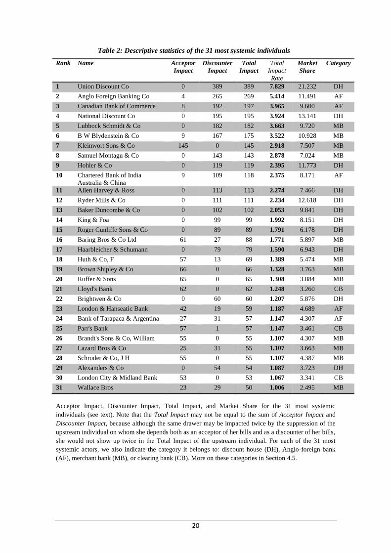
Banking Co with 5.41%), while as many as 597 upstream actors have no impact at all. Table 2

provides more details on the 31 individuals who have a Total Impact Rate exceeding 1%. As

also shown in Figure 4, Union Discount Co is by far the biggest actor in the network, with a

market share of 21.23%. However, its removal impacts only 7.83% of the network (389 actors),

which is relatively low. The following five individuals in the ranking are either pure discounters

or hybrids who mainly play the role of discounters. The most systemic pure acceptor,

Kleinworth Sons & Co, only comes seventh in the general ranking, with an Absolute Impact

Rate of 2.92% in spite of a market share of 7.51%. Thus, the ranking appears to be dominated

19

by discounters, and esp. by discount houses (money market funds). We shall come back to this

issue in Section 4.5.

20

Table 2: Descriptive statistics of the 31 most systemic individuals 2

Rank Name Acceptor

Impact

Discounter

Impact

Total

Impact

Total

Impact

Rate

Market

Share

Category

1 Union Discount Co 0 389 389 7.829 21.232 DH

2 Anglo Foreign Banking Co 4 265 269 5.414 11.491 AF

3 Canadian Bank of Commerce 8 192 197 3.965 9.600 AF

4 National Discount Co 0 195 195 3.924 13.141 DH

5 Lubbock Schmidt & Co 0 182 182 3.663 9.720 MB

6 B W Blydenstein & Co 9 167 175 3.522 10.928 MB

7 Kleinwort Sons & Co 145 0 145 2.918 7.507 MB

8 Samuel Montagu & Co 0 143 143 2.878 7.024 MB

9 Hohler & Co 0 119 119 2.395 11.773 DH

10 Chartered Bank of India

Australia & China

9 109 118 2.375 8.171 AF

11 Allen Harvey & Ross 0 113 113 2.274 7.466 DH

12 Ryder Mills & Co 0 111 111 2.234 12.618 DH

13 Baker Duncombe & Co 0 102 102 2.053 9.841 DH

14 King & Foa 0 99 99 1.992 8.151 DH

15 Roger Cunliffe Sons & Co 0 89 89 1.791 6.178 DH

16 Baring Bros & Co Ltd 61 27 88 1.771 5.897 MB

17 Haarbleicher & Schumann 0 79 79 1.590 6.943 DH

18 Huth & Co, F 57 13 69 1.389 5.474 MB

19 Brown Shipley & Co 66 0 66 1.328 3.763 MB

20 Ruffer & Sons 65 0 65 1.308 3.884 MB

21 Lloyd's Bank 62 0 62 1.248 3.260 CB

22 Brightwen & Co 0 60 60 1.207 5.876 DH

23 London & Hanseatic Bank 42 19 59 1.187 4.689 AF

24 Bank of Tarapaca & Argentina 27 31 57 1.147 4.307 AF

25 Parr's Bank 57 1 57 1.147 3.461 CB

26 Brandt's Sons & Co, William 55 0 55 1.107 4.307 MB

27 Lazard Bros & Co 25 31 55 1.107 3.663 MB

28 Schroder & Co, J H 55 0 55 1.107 4.387 MB

29 Alexanders & Co 0 54 54 1.087 3.723 DH

30 London City & Midland Bank 53 0 53 1.067 3.341 CB

31 Wallace Bros 23 29 50 1.006 2.495 MB

Acceptor Impact, Discounter Impact, Total Impact, and Market Share for the 31 most systemic

individuals (see text). Note that the Total Impact may not be equal to the sum of Acceptor Impact and

Discounter Impact, because although the same drawer may be impacted twice by the suppression of the

upstream individual on whom she depends both as an acceptor of her bills and as a discounter of her bills,

she would not show up twice in the Total Impact of the upstream individual. For each of the 31 most

systemic actors, we also indicate the category it belongs to: discount house (DH), Anglo-foreign bank

(AF), merchant bank (MB), or clearing bank (CB). More on these categories in Section 4.5.

21

Therefore, our upper-bound estimates of the degree of unsubstitutability of actors in the early-

20th-century global financial network suggest that, contrary to nowadays’ interbank networks

(Gai and Kapadia, 2010), the system was not prone to the “robust-yet-fragile” tendency, as it

did not feature any “mega-hub”. This is our baseline result.

The second feature emerging from Figure 4 is that the vast majority of dots are situated well

below the diagonal of the graph: only individuals with very low Market Share values are close

to the diagonal. Individuals are plotted on the diagonal when, following their removal, 100% of

their downstream actors lose market access: the farther the dots are from the diagonal, the lesser

the degree of dependence of their downstream actors. The figure suggests that most upstream

individuals “punch well below their weight” in terms of their unsubstitutability for their

downstream actors. We investigate this issue in Section 4.4.

4.4. Local systemicness

We define local systemicness an individual’s degree of unsubstitutability for the downstream

actors who are connected to it through one or more chains. We compute for each individual i:

(a) the Acceptor Local Impact Rate ALocImpRi = AImpi / (Ani -1) , where AImpi is the

Acceptor Impact and Ani is the number of partners (number of actors involved in the same bills)

of i when i plays the role of acceptor; (b) the Discounter Local Impact Rate DLocImpRi =

DImpi / (Dni -1) , where DImpi is the Discounter Impact and Dni is the number of partners of i

when i plays the role of discounter; and (c) the Local Impact Rate LocImpRi = TImpi / (ni -1),

where TImpi is the Total Impact and ni is the overall number of partners of i.

22

Figure 5: Node removal – Absolute vs Local systemicness 5

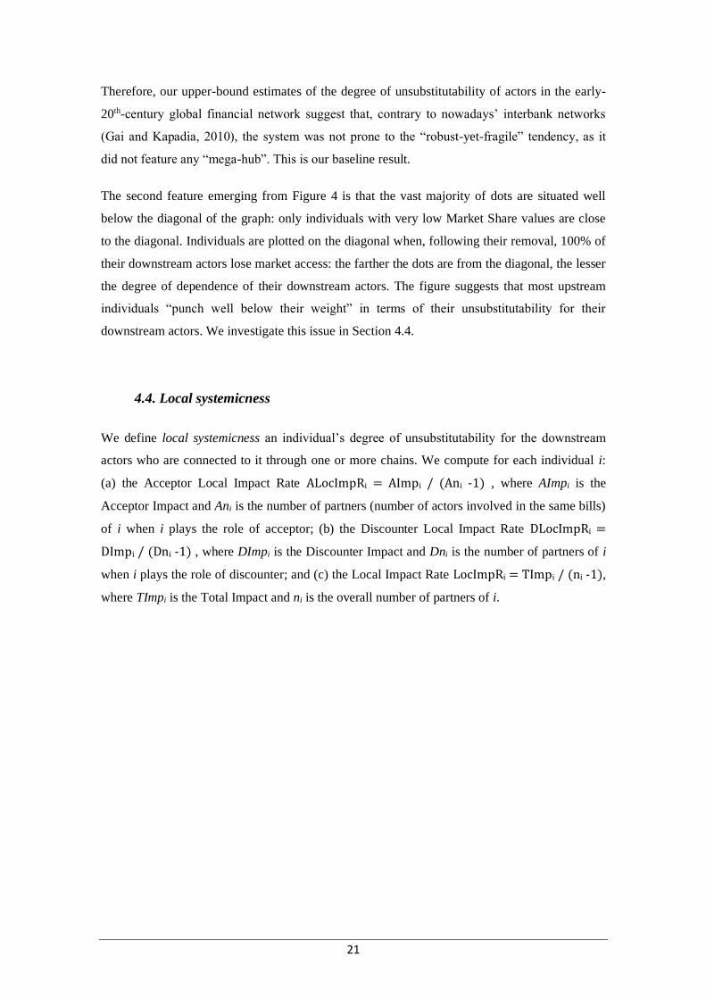
Total Impact Rate (x axis) and Local Impact Rate (y axis) of the 1,535 upstream actors.

Figure 5 shows that on average, local systemicness tends to be roughly stable (24.93%) across

levels of absolute systemicness. Unsurprisingly, there is a lot of dispersion in local systemicness

for low levels of absolute systemicness. This is because these actors are involved into a limited

number of chains, so there is a size effect on the rate. A simple illustration is provided by the

case of a discounter involved into one only bill: the discounter’s absolute systemicness is

always very low (because a maximum of two downstream actors are impacted by her removal),

but if both drawer and acceptor lose market access her local systemicness will be equal to 100%

– while it will be only equal to 0% if none of the two is impacted. Interestingly, in Figure 5

actors involved in the accepting business appear to display, on average, higher levels of local

systemicness than pure discounters. It is therefore legitimate to ask whether in the accepting

business (i.e., in bank-firm relationships), downstream actors’ level of dependence on upstream

ones might have been higher than in the discounting business (i.e., in bank-bank relationships).

23

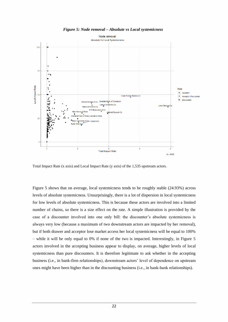
Figure 6: Local systemicness by acceptor-discounter roles 6

Number of partners as acceptor (light blue), Acceptor Local Impact (dark blue), number of partners as

discounter (light red), and Discounter Local Impact (dark red) for the 31 individuals with a Total Impact

Rate exceeding 1% (ranked according to their Total Impact).

In order to answer this question, Figure 6 compares the Acceptor Local Impact and the

Discounter Local Impact for the 31 actors with highest absolute systemicness (see Table 2). In

general, the Acceptor Local Impact Rate is actually higher than the Discounter Local Impact

Rate. Thus, downstream actors appear to have displayed a relatively higher level of dependence

on acceptors than on discounters. However, some exceptions did actually exist. For instance, we

can see in Figure 6 that the two individuals with the second and third highest absolute

systemicness, Anglo Foreign Banking Co and Canadian Bank of Commerce (two hybrid actors),

both displayed an Acceptor Local Rate that was lower than their Discounter Local Rate.

24

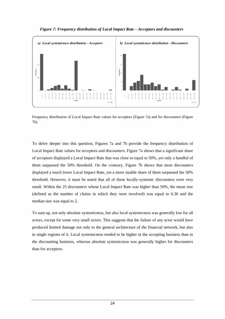
Figure 7: Frequency distribution of Local Impact Rate – Acceptors and discounters 7

Frequency distribution of Local Impact Rate values for acceptors (Figure 7a) and for discounters (Figure

7b).

To delve deeper into this question, Figures 7a and 7b provide the frequency distribution of

Local Impact Rate values for acceptors and discounters. Figure 7a shows that a significant share

of acceptors displayed a Local Impact Rate that was close or equal to 50%, yet only a handful of

them surpassed the 50% threshold. On the contrary, Figure 7b shows that most discounters

displayed a much lower Local Impact Rate, yet a more sizable share of them surpassed the 50%

threshold. However, it must be noted that all of these locally-systemic discounters were very

small. Within the 25 discounters whose Local Impact Rate was higher than 50%, the mean size

(defined as the number of chains in which they were involved) was equal to 6.36 and the

median size was equal to 2.

To sum up, not only absolute systemicness, but also local systemicness was generally low for all

actors, except for some very small actors. This suggests that the failure of any actor would have

produced limited damage not only to the general architecture of the financial network, but also

to single regions of it. Local systemicness tended to be higher in the accepting business than in

the discounting business, whereas absolute systemicness was generally higher for discounters

than for acceptors.

25

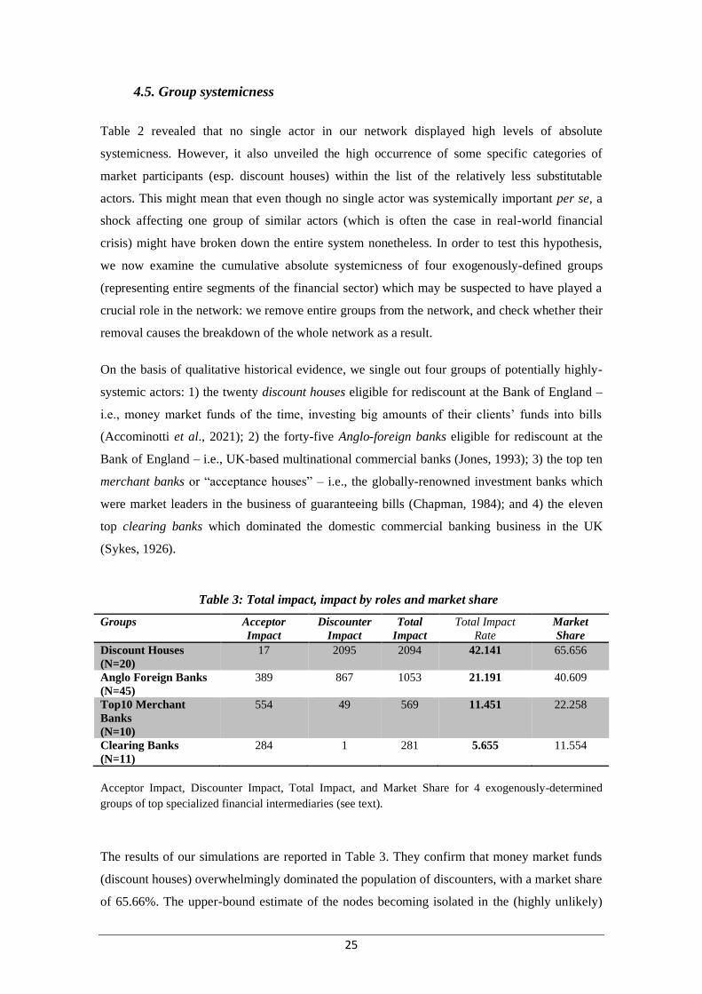
4.5. Group systemicness

Table 2 revealed that no single actor in our network displayed high levels of absolute

systemicness. However, it also unveiled the high occurrence of some specific categories of

market participants (esp. discount houses) within the list of the relatively less substitutable

actors. This might mean that even though no single actor was systemically important per se, a

shock affecting one group of similar actors (which is often the case in real-world financial

crisis) might have broken down the entire system nonetheless. In order to test this hypothesis,

we now examine the cumulative absolute systemicness of four exogenously-defined groups

(representing entire segments of the financial sector) which may be suspected to have played a

crucial role in the network: we remove entire groups from the network, and check whether their

removal causes the breakdown of the whole network as a result.

On the basis of qualitative historical evidence, we single out four groups of potentially highly-

systemic actors: 1) the twenty discount houses eligible for rediscount at the Bank of England –

i.e., money market funds of the time, investing big amounts of their clients’ funds into bills

(Accominotti et al., 2021); 2) the forty-five Anglo-foreign banks eligible for rediscount at the

Bank of England – i.e., UK-based multinational commercial banks (Jones, 1993); 3) the top ten

merchant banks or “acceptance houses” – i.e., the globally-renowned investment banks which

were market leaders in the business of guaranteeing bills (Chapman, 1984); and 4) the eleven

top clearing banks which dominated the domestic commercial banking business in the UK

(Sykes, 1926).

Table 3: Total impact, impact by roles and market share 3

Groups Acceptor

Impact

Discounter

Impact

Total

Impact

Total Impact

Rate

Market

Share

Discount Houses

(N=20)

17 2095 2094 42.141 65.656

Anglo Foreign Banks

(N=45)

389 867 1053 21.191 40.609

Top10 Merchant

Banks

(N=10)

554 49 569 11.451 22.258

Clearing Banks

(N=11)

284 1 281 5.655 11.554

Acceptor Impact, Discounter Impact, Total Impact, and Market Share for 4 exogenously-determined

groups of top specialized financial intermediaries (see text).

The results of our simulations are reported in Table 3. They confirm that money market funds

(discount houses) overwhelmingly dominated the population of discounters, with a market share

of 65.66%. The upper-bound estimate of the nodes becoming isolated in the (highly unlikely)

26

catastrophic scenario of a total destruction of this crucial segment of the financial sector is equal

to 42.14%. This is quite a significant damage, but it falls short of breaking down the entire

backbone of the financial network. All other groups display a much lower Total Impact Rate:

21.19% for Anglo-foreign banks, 11.45% for the top ten merchant banks, and 5.65% for the

clearing banks. Unsurprisingly, a linear relation appears to exist between Market Share and

Total Impact Rate. On the whole, even the removal of entire segments of the financial sector

does not entail the collapse of the network.

4.6. Geographic systemicness

Assessing the geographic systemicness of upstream actors is yet another way to study the

resilience of a system. Financial intermediaries in London might have been specialized along

geographic lines, and this might have been conducive to some form of dependence for some

regions on some specific actor to access to the market. Thus, if drawers from a region or a city

were used to access the market only via one acceptor and/or one discounter specialized in that

particular region or city, the failure of these actors would have implied the loss of the access to

the London bills market for this part of the world.

In order to test for this particular variant of local systemicness, we use the drawers’ location

data to test the dependence of cities around the world (617 in our database, including London

itself) on individual upstream actors to access to the London bill market. Similarly to previous

analyses, we identify the number of drawers who lose market access when an individual playing

the role of acceptor and/or discounter is removed. Naturally, all cities which are connected to

London only through one single chain are very vulnerable (257 cities), because they have an

absolute dependence on one acceptor and one discounter. Table 4 gives the frequency

distribution of our 617 cities according to the number of drawers they feature. It shows that

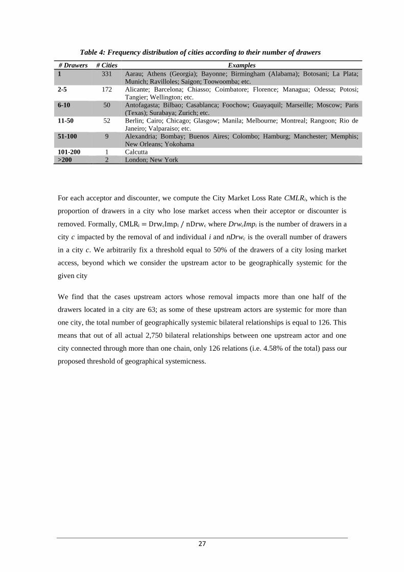
27

Table 4: Frequency distribution of cities according to their number of drawers 4

# Drawers # Cities Examples

1 331 Aarau; Athens (Georgia); Bayonne; Birmingham (Alabama); Botosani; La Plata;

Munich; Ravilloles; Saigon; Toowoomba; etc.

2-5 172 Alicante; Barcelona; Chiasso; Coimbatore; Florence; Managua; Odessa; Potosi;

Tangier; Wellington; etc.

6-10 50 Antofagasta; Bilbao; Casablanca; Foochow; Guayaquil; Marseille; Moscow; Paris

(Texas); Surabaya; Zurich; etc.

11-50 52 Berlin; Cairo; Chicago; Glasgow; Manila; Melbourne; Montreal; Rangoon; Rio de

Janeiro; Valparaiso; etc.

51-100 9 Alexandria; Bombay; Buenos Aires; Colombo; Hamburg; Manchester; Memphis;

New Orleans; Yokohama

101-200 1 Calcutta

>200 2 London; New York

For each acceptor and discounter, we compute the City Market Loss Rate CMLRi, which is the

proportion of drawers in a city who lose market access when their acceptor or discounter is

removed. Formally, CMLRi = DrwcImpi / nDrwc where DrwcImpi is the number of drawers in a

city c impacted by the removal of and individual i and nDrwc is the overall number of drawers

in a city c. We arbitrarily fix a threshold equal to 50% of the drawers of a city losing market

access, beyond which we consider the upstream actor to be geographically systemic for the

given city

We find that the cases upstream actors whose removal impacts more than one half of the

drawers located in a city are 63; as some of these upstream actors are systemic for more than

one city, the total number of geographically systemic bilateral relationships is equal to 126. This

means that out of all actual 2,750 bilateral relationships between one upstream actor and one

city connected through more than one chain, only 126 relations (i.e. 4.58% of the total) pass our

proposed threshold of geographical systemicness.

28

Figure 8: Impact of individuals and groups removal on cities 8

The figures show on the left the acceptors or discounters, and on the right the cities impacted by their

removal. The width of flux between individuals and cities represents the number of drawers who lose

market access, and the colour darkening the proportion of these drawers with respect to the total

population of drawers in the city. Figure 8a illustrates the 126 geographically systemic bilateral

relationships between single upstream individuals and cities. Figure 8b illustrates the 208 geographically

29

systemic bilateral relationships between groups of upstream individuals (i.e. segments of the financial

sector) and cities (see text).

The 126 geographically systemic actor-city relationships are represented in Figure 8a. The

figure shows that, for instance, if Alexanders & Co (who is connected to 3 out of the 5 drawers

in Newport) is removed, this city loses 60% of its access to the London market. Union Discount

is the most systemic actor for Boston, since 60% of the drawers depend on it. Similarly, Union

Discount Co is the most systemic actor of other cities like Curaçao or Trieste, since all drawers

of these cities depend on it. Some cities, like Yazoo City, are dependent on both an acceptor and

a discounter, and the removal of one of them makes the city lose access to the market. Figure 8a

shows that in some cases, some upstream actors played a geographically systemic role for some

cities. This was esp. the case for some actors who were specialized in financing trade with some

specific regions of the globe. For instance, the Anglo-foreign banks Anglo Foreign Banking Co

and Canadian Bank of Commerce appeared to play a systemic role for middle-sized (in terms of

number of drawers) cities located in Continental Europe and North America respectively, while

the merchant bank C Murdoch & Co appeared to play a systemic role for middle-sized cities

located in Africa. However, such cases of geographical “niches” appear to be the exception

rather than the rule. Interestingly, despite their huge market share, individual discount houses

like Union Discount Co “punch below their weight” in terms of geographic systemicness.

To further investigate this question, we also assess the geographic systemicness of the groups of

actors defined in Section 4.5 (i.e., the exogenously-defined crucial segments of the financial

sector). The results are presented in Figure 8b: they confirm the findings of Figure 8a. On the

one hand, in view of the presence of a number of individual geographical specialization niches,

Anglo-foreign banks and top merchant banks are systemic for many small-sized (in terms of

number of drawers) cities, but not for bigger ones. On the other hand, the removal of discount

houses as a group has a significant impact on 112 cities around the world, be them small,

middle-sized (such as Paris where it impacts slightly more than 50% of drawers, Manchester

with more than 75%, or Belfast with 100%), or big (such as New York where they impact

53.48% of drawers, or Calcutta with 61.93%). This means that only 45.16% of the bilateral

relationships between the group and one city can be seen as geographically systemic. In view of

the large market share of discount houses (65.66% of bills), this result is not particularly

impressive. Even in the (highly unlikely) catastrophic scenario in which the whole segment of

money market funds had disappeared, most cities would still have been able to keep their access

to the core of the global financial network.

30

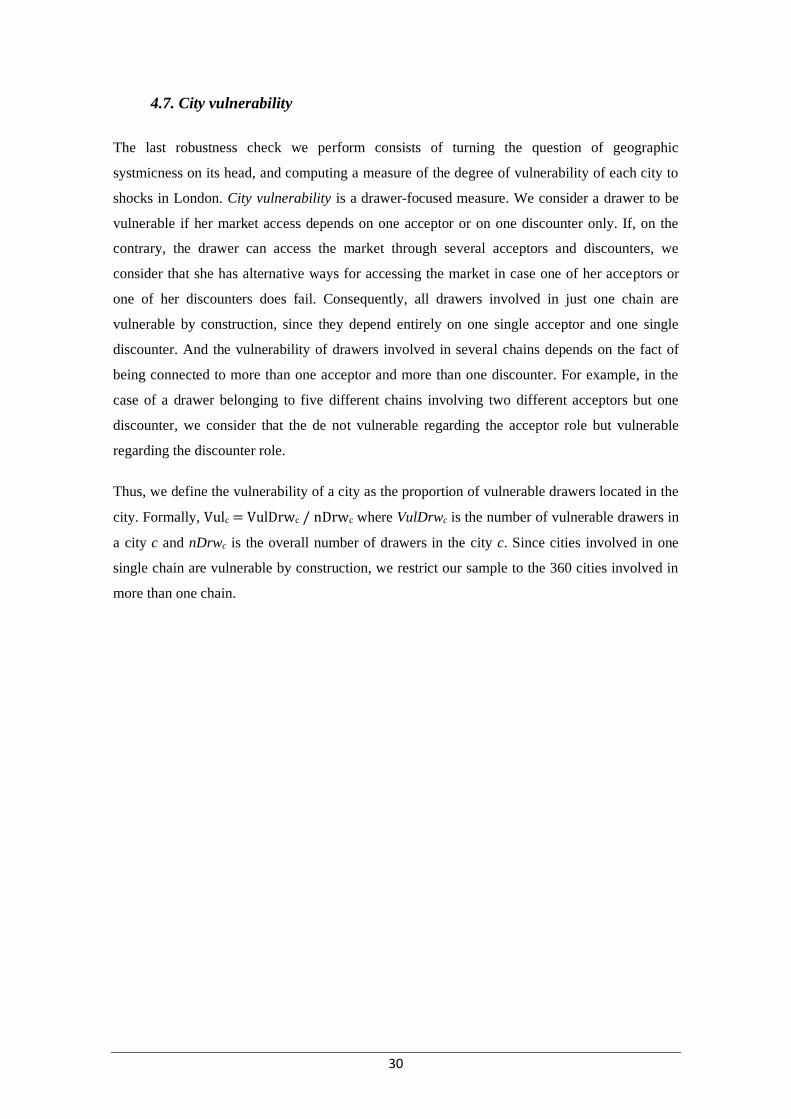
4.7. City vulnerability

The last robustness check we perform consists of turning the question of geographic

systmicness on its head, and computing a measure of the degree of vulnerability of each city to

shocks in London. City vulnerability is a drawer-focused measure. We consider a drawer to be

vulnerable if her market access depends on one acceptor or on one discounter only. If, on the

contrary, the drawer can access the market through several acceptors and discounters, we

consider that she has alternative ways for accessing the market in case one of her acceptors or

one of her discounters does fail. Consequently, all drawers involved in just one chain are

vulnerable by construction, since they depend entirely on one single acceptor and one single

discounter. And the vulnerability of drawers involved in several chains depends on the fact of

being connected to more than one acceptor and more than one discounter. For example, in the

case of a drawer belonging to five different chains involving two different acceptors but one

discounter, we consider that the de not vulnerable regarding the acceptor role but vulnerable

regarding the discounter role.

Thus, we define the vulnerability of a city as the proportion of vulnerable drawers located in the

city. Formally, Vulc = VulDrwc / nDrwc where VulDrwc is the number of vulnerable drawers in

a city c and nDrwc is the overall number of drawers in the city c. Since cities involved in one

single chain are vulnerable by construction, we restrict our sample to the 360 cities involved in

more than one chain.

31

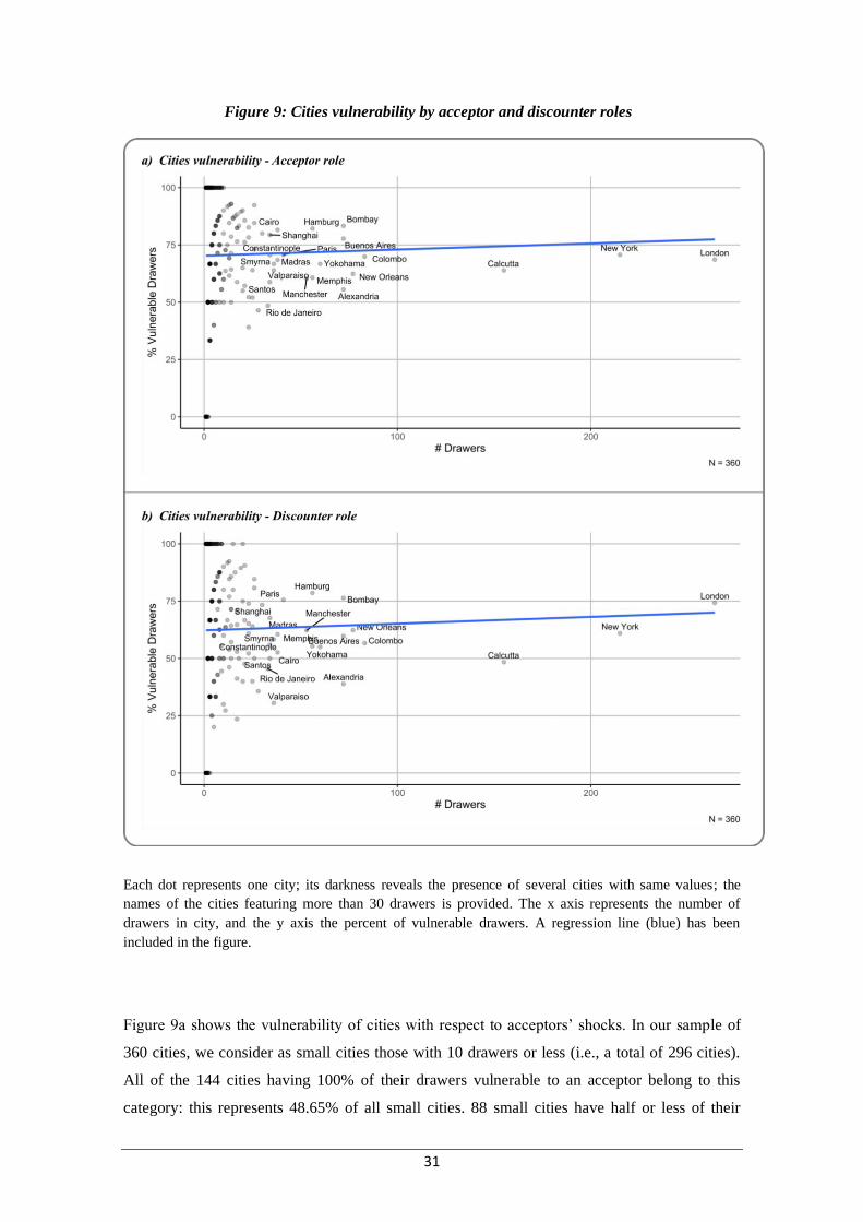
Figure 9: Cities vulnerability by acceptor and discounter roles 9

Each dot represents one city; its darkness reveals the presence of several cities with same values; the

names of the cities featuring more than 30 drawers is provided. The x axis represents the number of

drawers in city, and the y axis the percent of vulnerable drawers. A regression line (blue) has been

included in the figure.

Figure 9a shows the vulnerability of cities with respect to acceptors’ shocks. In our sample of

360 cities, we consider as small cities those with 10 drawers or less (i.e., a total of 296 cities).

All of the 144 cities having 100% of their drawers vulnerable to an acceptor belong to this

category: this represents 48.65% of all small cities. 88 small cities have half or less of their

32

drawers vulnerable: 50 of them have no vulnerable drawer at all (most of them have only one

drawer involved in several chains with several acceptors). Figure 9a also shows that no city with

more than 10 drawers is completely vulnerable, and the percent of vulnerable actors tends ≈

70% as the size of the city increases.

Figure 9b shows the vulnerability of cities with respect to discounters’ shocks. It shows that in

general, cities’ vulnerability with respect to discounters is lower than their vulnerability with

respect to acceptors. On the one hand, the number of cities that are 100% vulnerable to

discounters’ shocks is lower than for acceptors’, as it is equal to 115. However, 2 of these 115

cities (Port Said and Amsterdam) are middle-sized cities with more than 10 drawers (15 and 20

respectively). On the other hand, the number of cities with no vulnerable drawer grows to 60

(most of them have one only drawer involved in several chains with several discounters).

Another interesting fact is that 20 cities with one single drawer are resilient to acceptors’ shocks

but vulnerable to discounters’ ones. Similarly, among the 64 cities with more than 10 drawers,

12 exhibit more vulnerability to discounters’ shocks than to acceptors’: this is esp. the case for

cities located in the UK, such as London, Manchester, Belfast, or Bradford.

These findings confirm that in spite of the high concentration of the discounting business (in

which 20 discount houses detained a market share of 65.66%), the degree of unsubstitutability

of discounters (i.e., wholesale lenders) was lower than expected. Drawers (i.e., borrowing firms)

could generally pass through many alternative paths in order to access the London market;

often, they displayed a greater degree of dependence on acceptors (i.e., guarantors), whose

market share was nonetheless generally much lower than discounters’ (see above, section 4.3).

In a sense, a sort of trade-off existed in the banking system: on the one hand, guarantors had a

relatively higher degree of unsubstitutability for their customers, but this was compensated by a

lower market share; on the other hand, wholesale lenders had far bigger market shares, but this

was compensated by a relatively lower degree of unsubstitutability for their customers. This

trade-off appears to have stemmed from the fundamentally different characteristics of the

accepting and discounting businesses (Accominotti et al., 2021). The result was that, in spite of

a “funnel-shaped” demography, the macro structure early-20th-century global financial network

did not feature the sorts of “mega-hubs” found in present-day interbank networks, and were

therefore not prone to the “robust-yet-fragile” tendency.

6. Conclusions

We use a new database (hand-collected from archival sources) allowing to reconstruct the

complete network of financial interlinkages in the global sterling-denominated money market

during the calendar year 1906 (at the heyday of the first globalization). This database is valuable

33

under many respects: it consists of truly observed (and not estimated) linkages; it is one of the

very first historical databases on financial networks; to the best of our knowledge, it is the first

one to cover a core global money market; and it is one of the very few available databases

covering both bank-bank and bank-firm relationships. We apply very simple shock simulation

techniques (node removal) to obtain upper-bound estimates of the unsubstitutability of

intermediaries in the network. In contrast to the multilayer approach adopted by the literature in

order to analyse the interaction between bank-bank and bank-firm networks, this methodology

allows us keeping track of actual chains and of the role of gatekeepers in connecting borrowing

firms with lending banks.

When applied to contemporary financial networks, this kind of simulation leads to a breakdown

of the network’s connectivity as central nodes are removed (Pröpper et al., 2008), thus pointing

to a high level of unsubstitutability of a few systemic actors. In stark contrast, we find that in no

case the removal of any node leads to major damages to the network structure, as only very few

actors get isolated. This result is robust to several specifications of the shock simulations. All

this allows us concluding that, in stark contrast to today, during the first globalization no

intermediary had high levels of unsubstitutability in the global financial network. This means

that a financial network deprived of systemic actors can exist and did actually exist at one of the

highest times of international economic development.

This conclusion has important implications for regulators. In our historical companion paper

(Accominotti et al., 2021), we explain that the specific characteristics of the monetary

instruments that was at the basis of the global financial system (the bill of exchange) provided

incentives for gatekeepers (guarantors) to engage into information-production activities, and this

generated diseconomies of scale in their business, which was akin to relationship banking (Boot,

2000; Stein, 2002). On this basis, we speculate that the low systemicness of intermediaries was

the outcome of the specific design of the money market instruments used in those times. As a

matter of fact, 19th-century regulators were indeed adamant about the superiority of bills of

exchange from a supervisory viewpoint (Ugolini, 2017). If regulators want to escape the “too-

unsubstitutable-to-fail” trap, they should therefore start from the microstructure of financial

market and try to design instruments providing disincentives to concentration. As always, the

devil is in the details.

34

References

Accominotti, O., Ugolini, S. (Forthcoming) International Trade Finance from the Origins to the

Present: Market Structures, Regulation, and Governance. In Brousseau, E., Glachant,

J.M. and Sgard, J. (eds.), The Oxford Handbook of Institutions of International

Economic Governance and Market Regulation. Oxford University Press.

Accominotti, O., Lucena-Piquero, D., Ugolini, S. (2021) The origination and distribution of

money market instruments: sterling bills of exchange during the first globalization. The

Economic History Review.

Acemoglu, D., Ozdaglar, A., Tahbaz-Salehi, A. (2015) Systemic Risk and Stability in Financial

Networks. American Economic Review, 105(2), 564–608.

Albert, R., Jeong, H., Barabási, A.L. (2000) Error and Attack Tolerance of Complex Networks.

Nature, 406(6794), 378–382.

Allen, F., Babus, A. (2009) Networks in Finance. In Kleindorfer, P.R., Wind, Y.R. and Gunther,

R.E. (eds.), The Network Challenge: Strategy, Profit, and Risk in an Interlinked World.

Prentice Hall, pp. 367–381.

Allen, F., Gale, D. (2000) Financial Contagion. Journal of Political Economy, 108(1), 1–33.

Anand, K., Lelyveld, I. van, Banai, Á., Friedrich, S., Garratt, R., Hałaj, G., Fique, J., Hansen, I.,

Jaramillo, S.M., Lee, H., Molina-Borboa, J.L., Nobili, S., Rajan, S., Salakhova, D.,

Silva, T.C., Silvestri, L., de Souza, S.R.S. (2018) The Missing Links: A Global Study

on Uncovering Financial Network Structures from Partial Data. Journal of Financial

Stability, 35, 107–119.

Basel Committee on Banking Supervision (2013) Global Systemically Important Banks:

Updated Assessment Methodology and the Higher Loss Absorbency Requirement

(Technical Report). Bank for International Settlements.

Basel Committee on Banking Supervision (2018) Global Systemically Important Banks:

Revised Assessment Methodology and the Higher Loss Absorbency Requirement

(Technical Report). Bank for International Settlements.

Battiston, F., Cencetti, G., Iacopini, I., Latora, V., Lucas, M., Patania, A., Young, J.G., Petri, G.

(2020) Networks beyond Pairwise Interactions: Structure and Dynamics. Physics

Reports, 874, 1–92.

Battiston, S., Gatti, D.D., Gallegati, M., Greenwald, B., Stiglitz, J.E. (2012a) Default Cascades:

When Does Risk Diversification Increase Stability? Journal of Financial Stability, 8(3),

138–149.

Battiston, S., Gatti, D.D., Gallegati, M., Greenwald, B., Stiglitz, J.E. (2012b) Liaisons

Dangereuses: Increasing Connectivity, Risk Sharing, and Systemic Risk. Journal of

Economic Dynamics and Control, 36(8), 1121–1141.

Battiston, S., Martinez-Jaramillo, S. (2018) Financial Networks and Stress Testing: Challenges

and New Research Avenues for Systemic Risk Analysis and Financial Stability

Implications. Journal of Financial Stability, 35, 6–16.

Bech, M.L., Atalay, E. (2010) The Topology of the Federal Funds Market. Physica A:

Statistical Mechanics and its Applications, 389(22), 5223–5246.

Benoit, S., Hurlin, C., Pérignon, C. (2019) Pitfalls in Systemic-Risk Scoring. Journal of

Financial Intermediation, 38, 19–44.

35

Blasques, F., Bräuning, F., Van Lelyveld, I. (2015) A Dynamic Network Model of the

Unsecured Interbank Lending Market (Working Paper No. 491). Bank for International

Settlements.

Bonacich, P., Holdren, A.C., Johnston, M. (2004) Hyper-Edges and Multidimensional

Centrality. Social Networks, 26(3), 189–203.

Boss, M., Elsinger, H., Summer, M., Thurner, S. (2004) Network Topology of the Interbank

Market. Quantitative Finance, 4(6), 677–684.

Caccioli, F., Barucca, P., Kobayashi, T. (2017) Network Models of Financial Systemic Risk: A

Review. Journal of Computational Social Science, 1(1), 81–114.

Cai, J., Eidam, F., Saunders, A., Steffen, S. (2018) Syndication, Interconnectedness, and

Systemic Risk. Journal of Financial Stability, 34, 105–120.

Chapman, S. (1984) The Rise of Merchant Banking. Allen & Unwin, London.

Chinazzi, M., Fagiolo, G., Reyes, J.A., Schiavo, S. (2013) Post-Mortem Examination of the

International Financial Network. Journal of Economic Dynamics and Control, 37(8),

1692–1713.

Cohen, R., Havlin, S. (2010) Complex Networks: Structure, Robustness and Function.

Cambridge University Press.

Craig, B., Peter, G. von (2014) Interbank Tiering and Money Center Banks. Journal of

Financial Intermediation, 23(3), 322–347.

Criado, R., Romance, M., Vela-Pérez, M. (2010) Hyperstructures: A New Approach to

Complex Systems. International Journal of Bifurcation and Chaos, 20(03), 877–883.

Degryse, H., Nguyen, G. (2004) Interbank Exposures: An Empirical Examination of Systemic

Risk in the Belgian Banking System (Working Paper No. 43). National Bank of

Belgium.

Eisenberg, L., Noe, T.H. (2001) Systemic Risk in Financial Systems. Management Science,

47(2), 236–249.

Espinosa-Vega, M., Solé, J. (2010) Cross-Border Financial Surveillance: A Network

Perspective (Working Paper No. 10/105). International Monetary Fund.

Estrada, E., Rodríguez-Velázquez, J.A. (2006) Subgraph Centrality and Clustering in Complex

Hyper-Networks. Physica A: Statistical Mechanics and its Applications, 364, 581–594.

Freixas, X., Parigi, B.M., Rochet, J.C. (2000) Systemic Risk, Interbank Relations, and Liquidity

Provision by the Central Bank. Journal of Money, Credit and Banking, 32(3), 611–638.

Fricke, D., Lux, T. (2015a) Core-Periphery Structure in the Overnight Money Market: Evidence

from the e-MID Trading Platform. Computational Economics, 45(3), 359–395.

Fricke, D., Lux, T. (2015b) On the Distribution of Links in the Interbank Network: Evidence

from the e-MID Overnight Money Market. Empirical Economics, 49(4), 1463–1495.

Furfine, C.H. (1999) The Microstructure of the Federal Funds Market. Financial Markets,

Institutions & Instruments, 8(5), 24–44.

Gai, P., Kapadia, S. (2010) Contagion in Financial Networks. Proceedings of the Royal Society

A: Mathematical, Physical and Engineering Sciences, 466(2120), 2401–2423.

Glasserman, P., Young, H.P. (2015) How Likely Is Contagion in Financial Networks? Journal

of Banking & Finance, 50, 383–399.

Glasserman, P., Young, H.P. (2016) Contagion in Financial Networks. Journal of Economic

Literature, 54(3), 779–831.

36

Hale, G., Kapan, T., Minoiu, C. (2016) Crisis Transmission in the Global Banking Network

(Working Paper No. 16/91). International Monetary Fund.

Iori, G., Mantegna, R.N. (2018) Empirical Analyses of Networks in Finance. In Hommes, C.

and LeBaron, B. (eds.), Handbook of Computational Economics. Elsevier, pp. 637–685.

Iori, G., Mantegna, R.N., Marotta, L., Miccichè, S., Porter, J., Tumminello, M. (2015)

Networked Relationships in the E-MID Interbank Market: A Trading Model with

Memory. Journal of Economic Dynamics and Control, 50, 98–116.

Iori, G., Masi, G.D., Precup, O.V., Gabbi, G., Caldarelli, G. (2008) A Network Analysis of the

Italian Overnight Money Market. Journal of Economic Dynamics and Control, 32(1),

259–278.

Jones, G. (1995) British Multinational Banking, 1830-1990. Oxford University Press, Oxford.

Kapoor, K., Sharma, D., Srivastava, J. (2013) Weighted Node Degree Centrality for

Hypergraphs. In 2013 IEEE 2nd Network Science Workshop (NSW). pp. 152–155.

Li, D., Zhang, Q., Zio, E., Havlin, S., Kang, R. (2015) Network Reliability Analysis Based on

Percolation Theory. Reliability Engineering & System Safety, 142, 556–562.

Lux, T. (2016) A Model of the Topology of the Bank – Firm Credit Network and Its Role as

Channel of Contagion. Journal of Economic Dynamics and Control, 66, 36–53.

Martinez-Jaramillo, S., Alexandrova-Kabadjova, B., Bravo-Benitez, B., Solórzano-Margain,

J.P. (2014) An Empirical Study of the Mexican Banking System’s Network and Its

Implications for Systemic Risk. Journal of Economic Dynamics and Control, 40, 242–

265.

Masi, G.D., Fujiwara, Y., Gallegati, M., Greenwald, B., Stiglitz, J.E. (2011) An Analysis of the

Japanese Credit Network. Evolutionary and Institutional Economics Review, 7(2), 209–

232.

Masi, G.D., Gallegati, M. (2011) Bank–Firms Topology in Italy. Empirical Economics, 43(2),

851–866.

Minoiu, C., Kang, C., Subrahmanian, V.S., Berea, A. (2015) Does Financial Connectedness

Predict Crises? Quantitative Finance, 15(4), 607–624.

Minoiu, C., Reyes, J.A. (2013) A Network Analysis of Global Banking: 1978–2010. Journal of

Financial Stability, 9(2), 168–184.

Mistrulli, P.E. (2011) Assessing Financial Contagion in the Interbank Market: Maximum

Entropy versus Observed Interbank Lending Patterns. Journal of Banking & Finance,

35(5), 1114–1127.

Müller, J. (2006) Interbank Credit Lines as a Channel of Contagion. Journal of Financial

Services Research, 29(1), 37–60.

Newman, M.E.J. (2003) The Structure and Function of Complex Networks. SIAM Review,

45(2), 167–256.

O’Rourke, K.H., Williamson, J.G. (2002) When Did Globalisation Begin? European Review of

Economic History, 6(1), 23–50.

Pröpper, I., Marc Van Lelyveld, Heijmans, R. (2008) Towards a Network Description of

Interbank Payment Flows (Working Paper No. 177/2008). De Nederlandsche Bank.

Sheldon, G., Maurer, M. (1998) Interbank Lending and Systemic Risk: An Empirical Analysis

for Switzerland. Swiss Journal of Economics and Statistics, 134, 685–704.

Silva, T.C., Alexandre, M. da S., Tabak, B.M. (2018) Bank Lending and Systemic Risk: A

37

Financial-Real Sector Network Approach with Feedback. Journal of Financial Stability,

38, 98–118.

Soramäki, K., Bech, M.L., Arnold, J., Glass, R.J., Beyeler, W.E. (2007) The Topology of

Interbank Payment Flows. Physica A: Statistical Mechanics and its Applications,

379(1), 317–333.

Sykes, J. (1926) The Amalgamation Movement in English Banking, 1825-1925. King, London.

Temizsoy, A., Iori, G., Montes-Rojas, G. (2015) The Role of Bank Relationships in the

Interbank Market. Journal of Economic Dynamics and Control, 59, 118–141.

Ugolini, S. (2017) The Evolution of Central Banking: Theory and History. Palgrave Macmillan

UK.

Upper, C. (2011) Simulation Methods to Assess the Danger of Contagion in Interbank Markets.

Journal of Financial Stability, 7(3), 111–125.

Upper, C., Worms, A. (2004) Estimating Bilateral Exposures in the German Interbank Market:

Is There a Danger of Contagion? European Economic Review, 48(4), 827–849.

Wetherilt, A., Zimmermann, P., Soramäki, K. (2010) The Sterling Unsecured Loan Market

during 2006-08: Insights from Network Theory (Working Paper No. 398). Bank of

England.

38