studying statewide political campaigns · studying the advertising strategies of statewide...

Studying Statewide Political Campaigns

R. Michael Alvarez and Alexandra Shankster

TH E R E I S L I T T L E I N T H E AC A D E M I C literature about the dynamics ofcampaign advertising strategies and their effects on candidate electoralsuccess. While there have been theoretical and empirical studies of cam-paign strategy (Ferejohn and Noll 1978; Skarpedas and Grofman 1995;Glazer 1990) and scattered treatments of candidate advertising strategies(Roddy and Garramone 1988; Merritt 1984), our lack of understanding ofthe dynamics of advertising strategies has led some to wonder how much“campaigns matter” (Finkel 1993).

The difAculty in examining campaign dynamics stems from the lackof consistent data on candidate advertisements (West 1993). What little isknown about campaign advertisements comes from selective sampling oftelevision advertisements from presidential campaigns (West 1993) or fromexperimental studies (Ansolabehere et al. 1994; Ansolabehere and Iyengar1995; Garramone 1985; Garramone et al. 1990). Presidential campaigns,however, have several characteristics that make them ill-suited for study-ing the effects of advertising strategies. As Lau and Pomper note, presiden-tial campaigns feature the most prominent political Agures, who are lesslikely to be “redeAned” by an opponent’s attack advertisement. Further,presidential candidates enjoy much more media exposure than do Senateor gubernatorial candidates (Lau and Pomper 2002). Most important, thereis little variation in advertising strategies and the intensity of advertisingacross presidential campaigns. Finally, there is a very limited sample ofpresidential elections.

In this essay, we concentrate our analysis on two statewide races heldin California. There recently has been some interest in studying statewide

307

campaigns, largely because they do provide an important new resource forstudying political campaigns (Lau and Pomper 2002; Dalager 1996; Freed-man and Goldstein 1999; Sellers 1998; West 1993). In campaigns for ofAcessuch as state governor, U.S. Senate, and other statewide seats, there exists agreat variety of campaigns and advertising strategies. The intensity ofstatewide races varies enormously, both within states and over time. Bystudying the advertising strategies of statewide campaigns, the quasi-exper-imental setting produces a natural experiment in which we may, in effect,study both dosage and treatment effects of campaign advertising.

In this essay we analyze data collected during the Anal eight weeksof two statewide campaigns in California during 1994: the races for gover-nor and Senate. The campaigns were hard fought in that year and providean interesting laboratory in which to study intense campaigns over time andto compare the advertising strategies between races. We Arst begin by pre-senting data from the television advertisements from these two races. Thisdatabase of television advertisements from the last eight weeks of theseraces provides a unique opportunity to examine the strategies used in eachcampaign as candidates tried to get their messages through to the same vot-ers. Next, we turn to the politically relevant questions: Did these advertise-ments matter? Did the messages the candidates sent through their televisionadvertisements inBuence the electorate? To answer these questions, we usetwo sets of polling data from this election to see whether these televisionadvertisements effectively communicated the messages of each candidate tothe intended audience. We conclude with ways to improve the analysis ofpolitical campaigns by concentrating on suggestions for studying voter re-sponse to multiple campaign stimuli in one election year.

Data and Methods

We draw upon two sources of data in this essay. Both are taken from an in-tensive analysis of campaign television advertising. The Arst set containsadvertisements from the 1994 California Senate race and the second, fromthe 1994 California governor’s race. During the Anal eight weeks of the1994 general election campaign, we videotaped prime-time television(6:00 p.m.–midnight) from the two most highly rated television channelsin Los Angeles—KABC and KNBC. From these tapes, we obtained a day-by-day time-series of all television advertisements aired during this periodby the four major party candidates for these ofAces: Pete Wilson and Kath-

308 Capturing Campaign Effects

leen Brown in the governor’s race and Dianne Feinstein and Michael Huf-Angton in the Senate race.1

In total, there were 682 advertisements aired during these weeks onthese two stations, 340 from KABC and 342 from KNBC. This database isorganized by individual advertisements, as we know both the day and theevening program during which each advertisement was aired. In total, 177advertisements were aired by Wilson, 77 by Brown, 212 by HufAngton,and 216 by Feinstein.

Importantly, candidate advertising is a method whereby a candidatetries to convey his or her message to an audience. Because a contested po-litical campaign necessarily involves two or more candidates, an advertise-ment always focuses on one of the following: the candidate sponsoring theadvertisement, the sponsoring candidate’s opponent, or both the sponsor-ing candidate and the opponent in a comparative advertisement. As we shallshow, the nature of the advertisement’s focus often determines the tone:positive, negative, or a contrast of the candidates.2 Thus, each advertise-ment in this database was analyzed by content to determine the sponsoringcandidate, the tone (positive, attack, or contrast), the focus (whether it wasprimarily focused on the sponsoring candidate, the opponent, or a compar-ative advertisement), and the general theme of the advertisement (policy is-sues, personality and background, or policy record).3

This coding scheme provides an excellent analytical tool withwhich to understand the motivations of the candidates during their cam-paigns. In particular, by studying the tone and focus of television advertise-ments, we can better understand the strategies candidates use at differentpoints in their campaigns. Positive statements about oneself are used by acandidate to sell his or her candidacy to an uncertain or skeptical elec-torate. Attack advertisements focus on the mistakes of one’s opponent andcan induce uncertainty or reduce the electorate’s affect for the opponent.Comparative advertisements, designed to draw contrasts between the can-didate and the opponent, are used to accomplish the goals of both positiveand attack advertisements simultaneously.

Furthermore, as we shall see subsequently, there are repeatedly ob-served dynamics involved in candidate advertising. Candidates generallystart the campaign using positive strategies, especially when they are intro-ducing themselves to an uncertain or skeptical electorate. Positive adver-tisements help develop positive effect and rapport between the electorateand the candidate, help the candidate in building his or her electorate base,

Studying Statewide Political Campaigns 309

and, Anally, help attract swing voters. Negative advertisements, on theother hand, tend to be used later in the campaign. These advertisementscan have unpredictable consequences, as candidates who are perceived tohave crossed some threshold of negativity in the attack may suffer a back-lash. Therefore, negative advertisements are used when the potential ofbacklash can be minimized, generally late in the race and quite often onlywhen a candidate is falling behind in the polls. Comparative advertise-ments, which combine aspects of positive and attack strategies, are usedthroughout the race.

To match the campaign strategies determined using this databasewith voter responses, we use polling data from this election to probe thetwo ways in which television advertisements might inBuence voters. First,they may inBuence the weights that voters place on various issues. We usean exit poll conducted by the Los Angeles Times to examine how votersweighted issues in their voting behavior in this election. While this exitpoll covered the entire state on Election Day, it contained a large over-sampling of voters in the Los Angeles area. One important note of caution,however, in interpreting our results is the absence of any data on the view-ing habits of respondents. As noted in a study by Freedman and Goldstein,exposure to any particular campaign advertisement is a function of boththe frequency with which the advertisement was aired and the amount oftelevision watched by the respondent (Freedman and Goldstein 1999).Ideally, we would have access to the latter and be able to incorporate itinto our analysis. However, as this data was not available at that time, weinstead estimate our results using only the frequency with which an adver-tisement was aired. We believe this is partially justiAed, as, regardless ofwho actually viewed the advertisement, candidates employed speciAc cam-paign strategies, acting as if voters were watching them.

Further, in their study, Freedman and Goldstein used the Polaris AdDetecter, a tracking system that monitors political activity throughout theyear. They found that, during the 1997 Virginia gubernatorial election,candidates were most likely to air advertisements during the daytime andearly evening hours, concentrating most heavily on the half hour leadingup to prime-time television (Freedman and Goldstein 1999). Therefore, wefeel our analysis is likely to accurately capture the campaign tactics em-ployed by candidates, because, as noted earlier, we analyzed advertise-ments aired between 6:00 p.m. and midnight.

Second, advertisements may inBuence voter evaluations of candi-


dates over the course of the campaign season. We use three Field Pollsfrom the general election campaign in 1994. These are telephone pollsconducted statewide in July, September, and October 1994. As they arestatewide samples, they provide an opportunity to examine the ways inwhich voters evaluated the candidates throughout the 1994 general elec-tion in California. Further, we may use these polls to determine whetherchanges in candidate evaluations correspond to changes in the mediastrategies of the candidates.

The Advertising Strategies in the 1994 Campaign

Cumulative Results

We begin by examining the general tone of candidate television advertise-ments in this election—whether the advertisements were primarily posi-tive or negative or contrasted the candidates. We deAne a positive adver-tisement as one in which a candidate mentions factual information in anonderogatory manner. Positive television advertisements, then, are prima-rily by one candidate about his or her own issue position, record, or per-sonal background. We used the Surlin and Gordon (1977) operationaliza-tion of negative advertisements: a negative advertisement attacks theopponent’s personality, policy platform, or party. To deAne contrast adver-tisements, we used Merritt’s (1984) operationalization. Here, comparativeadvertisements highlight differences between candidates in order to high-light the superior qualities of the sponsor; these differ from negative adver-tisements that highlight the inferiority of the opponent.

Table 1 summarizes the relative frequencies of advertisement focusfor each candidate (the gubernatorial candidates are in the left panels; theSenate candidates are in the right panels). These results provide mixed sup-port for the common wisdom about the strategic interaction between in-cumbents and challengers. Jacobson (1992) summarizes the common typesof advertising strategies for challengers as attempts “to convince people oftheir own virtues—at a minimum, that they are qualiAed for the ofAce—but they are not likely to get far without directly undermining support forthe incumbent” (87). Incumbents, however, are commonly believed to ig-nore opponents when they feel safe but may strike preemptively at thechallenger if feeling vulnerable (96).

It is apparent that the focus strategies within each race are quitesimilar. In contrast, the focus strategies across races are quite distinct. It is


possible that the vast difference observed in patterns is candidate driven orcontext speciAc. Feinstein went negative early in the race; HufAngton thentried to protect himself by retaliating in kind. This tit-for-tat advertisingstrategy grew quite ugly, and by the end of the campaign, both candidateswere primarily airing attack advertisement after attack advertisement.

In contrast, the gubernatorial campaign followed a more typicalpattern. Wilson, the incumbent, aired more advertisements than did Brown(Wilson aired 177 advertisements during this period while Brown aired77); however, both Brown and Wilson aired more positive than negativeadvertisements, thus conducting mainly positive campaigns (61 percent ofWilson’s 177 advertisements and 68 percent of Brown’s 77 advertisementswere coded as positive in tone). For Brown, this might have been a subop-timal strategy, as the literature repeatedly Ands that positive advertise-ments are less effective than negative advertisements. According toGuskind and Hangstrom (1988), it takes between Ave and ten viewings ofa positive advertisement before the information sinks in. In contrast, it onlytakes one to two viewings of a negative advertisement for the message tohave an impact on viewers.

Again, the Senate race differed greatly from the gubernatorial race.


TABLE 1. Candidates, Advertisement Type, and Content

Wilson Brown Feinstein Huffington

Advertisement typePositive 108 (61) 52 (68) 6 (3) 24 (11)Attack 63 (36) 23 (30) 158 (73) 108 (51)Contrast 6 (3) 2 (2) 52 (24) 80 (38)

Advertisement contentIssue 128 (72) 52 (68) 0 (0) 28 (13)Personal 7 (4) 0 (0) 206 (95) 28 (13)Record 42 (24) 25 (32) 10 (5) 156 (74)

IssuesTaxes 13 (7) 0 (0) 0 (0) 15 (10)Education 0 (0) 14 (18) 0 (0) 0 (0)Crime 56 (32) 0 (0) 6 (3) 28 (19)Immigration 66 (37) 0 (0) 0 (0) 19 (13)Ethics 0 (0) 0 (0) 39 (18) 89 (59)Morality 0 (0) 0 (0) 171 (79) 0 (0)Budget 0 (0) 23 (30) 0 (0) 0 (0)Economy 42 (24) 40 (52) 0 (0) 0 (0)

Note: Entries are the number of advertisements in each category, followed by the percentage of each typefor the specific candidate.

Michael HufAngton, the Republican challenger, aired attack advertise-ments about his opponent and comparative advertisements with almostequal frequency. He aired relatively few positive advertisements abouthimself. Dianne Feinstein, the Democratic incumbent, focused her adver-tisements almost exclusively on attacking HufAngton.

In contrast to Jacobson’s Andings, Wilson and Brown aired advertise-ment types in roughly equal proportions. Wilson, in airing mainly positiveadvertisements, followed the strategy normally associated with strong, se-cure incumbents. What makes this strategy an odd choice is that Wilsonshould have been anything but secure about his reelection prospects—six-teen months before the general election, he was losing by at least 20 per-cent in many polls! As late as July 1994, Wilson was in a statistical dead heatwith Brown (38.5 percent for Wilson, 42.7 percent for Brown, in the July1994 Field Poll). That the race was this close in the middle of the summer,moreover, should have led Brown to attempt to undermine support for Wil-son through negative advertising. However, Brown seems to have tried towin the race through primarily positive advertising, in the face of conven-tional wisdom.

Feinstein, the other incumbent, should have felt more secure, as shehad a slight lead over HufAngton before the general election heated up(44.4 percent for Feinstein, 39.0 percent for HufAngton). But in an envi-ronment characterized by uncertainty, Feinstein seems to have taken therisk averse strategy, mainly airing attack advertisements about her oppo-nent. Furthermore, the challengers in both races seem to have followed thecommon wisdom outlined by Jacobson (1992); Wilson predominately at-tacked Brown, while HufAngton used both attack and comparative adver-tisements in roughly equal proportions.

However, it is critical that we understand the content of these ad-vertisements to better examine candidate advertising strategies. Table 1also presents the breakdown of advertisement content into three generalcategories—whether the advertisement was primarily issue based, person-ality based, or record based—for each candidate. Both Wilson and Brown(left panels of table 1) focused heavily on issues in this race. Brown, how-ever, sought to focus attention on both Wilson’s record as governor and herown record as state treasurer. However, while the data in table 1 indicatethat issues were a primary focus of advertising by these two candidates, itis not clear how informative these issue advertisements were.

During the Senate race, HufAngton targeted Feinstein’s record as


incumbent senator, focusing mainly on her actions in ofAce. There was asmall amount of advertising by HufAngton, however, focusing on both is-sues and personalities. But Feinstein’s advertising strategy stands in clearcontrast to HufAngton’s—she poured almost all of her advertising into at-tacks about HufAngton’s personal background.

Next, we examined the speciAc issues raised by the candidates intheir advertising. We categorized all advertisements as having up to fourspeciAc themes. We then coded eight individual issues—taxes, education,crime, immigration, personal ethics, personal morality, state budget, andstate economy. We present the frequencies of issue mention across the fourcampaigns at the bottom of table 1.

The governor’s race focused on salient statewide issues. Wilson cam-paigned on the issues of illegal immigration, the state economy, crime, andtaxes, while Brown focused most of her issue discussion on the state budgetand economy. Wilson employed what the literature calls a “resonance strat-egy” (Johnson-Cartee and Copeland 1991; Combs 1979). This involves aseries of persuasive messages that are “harmonious” with the experiences ofthe audience. In other words, political consultants search for hot buttonsthat they can exploit in the campaign (Combs 1979). In 1994, the major hotbuttons were illegal immigration and crime, evidenced by the overwhelm-ing passage of the controversial initiative Proposition 187.

The Senate race, however, was much more personal in nature thanthe governor’s race. HufAngton spent most of his television advertisementtime discussing Feinstein’s personal ethics. To a much lesser degree, hebrought forward the more substantive issues of crime, illegal immigration,and taxes. Feinstein’s strategy was quite clear: She devoted an overwhelm-ing proportion of her advertising time on HufAngton’s personal moralityand ethics. The more substantive issues received little attention in Fein-stein’s television advertisements.

These tables produce a revealing portrait of the candidate strategiesin the 1994 California elections. A composite sketch of the cumulative ev-idence for each campaign’s strategy shows the following:

Wilson aired mostly positive television advertisements, focusing onhis own positions on issues. The issues he discussed most generallywere illegal immigration, the state economy, crime, and the statebudget. When Wilson went negative, it was strategically successful.

Brown ran attack advertisements, which did not focus on salientissues. She also ran advertisements personally attacking Wilson,


which, according to the literature, does win the favor of the elec-torate. She focused on the state economy and budget in heradvertisements.

Feinstein relied almost exclusively on attack advertisements aimedat HufAngton’s personal morality and ethics.

HufAngton ran mainly attack advertisements against Feinstein;however, he also aired some comparative advertisements. In gen-eral, HufAngton focused mainly on Feinstein’s personal ethics,but he also discussed crime, illegal immigration, and taxes.

By examining the cumulative evidence on the content and type oftelevision advertisements used by each candidate in this race, a compositesketch of each candidate’s advertisement strategy can easily be drawn.

In conclusion, the dramatic differences we observe in candidatestrategies by these four different statewide campaigns lead to an importantpoint: Despite the fact that each of these candidates was campaigningwithin exactly the same constituency, it is clear that each candidate be-lieved different issues needed to be emphasized. This is true even when welook at the issue focused within each race, especially Wilson’s and Brown’s.While there might be many explanations for these dramatic differences incampaign issue focus, it is important to note that the candidates were issu-ing different appeals to the same electorate.

The key question, then, is, Did the voters receive these messages?That is, did the candidates’ issue strategies connect with the electorate inways the candidates intended? Did voters realize that the candidates em-phasized different issues from each other? We return to these points later.

Dynamic Results

The analysis thus far has ignored the dynamic nature of our database ofcandidate television advertisements, which allows for an examination ofthe changing composition of each candidate’s television advertisementstrategy over the last eight weeks of the 1994 general election. In table 2we give the weekly frequency of advertisements by the four campaigns. Forthe two gubernatorial candidates, Wilson maintained a consistent level ofadvertising throughout the last two months of the election. While Brownemployed a similar strategy, surprisingly for a challenger, she aired fewadvertisements in the Anal, critical days of the election.

The Senate race stands in sharp contrast. There, HufAngton was on


the air consistently throughout the general election race, with an increasein advertising frequency in the last weeks of the election. Feinstein was noton the air in Los Angeles for the Arst week of the sample but advertisedheavily in the last week of the race.

In addition to examining the frequency of advertisements, we mayalso observe when the candidates “went negative” and at what points in thecampaign they were airing advertisements that were issue or personalitybased. In tables 3 and 4 we examine the weekly proportions of advertise-ments in each campaign by type (attack or positive in table 3) and by con-tent (issue, personality, or record in table 4).

In table 3 we uncover more details about the advertising strategiesof the candidates in this election year. In the Arst three weeks of this criti-cal period of the election year, Wilson’s advertisements were overwhelm-


TABLE 2. Candidate Advertising Share

Campaign Week

Candidate 1 2 3 4 5 6 7 8

Wilson 12 11 9 11 11 8 13 24Brown 13 13 5 16 18 12 18 5Huffington 6 8 8 8 17 13 16 24Feinstein 0 1 14 16 13 13 15 28

Note: Entries are the percentage of advertisements aired by each candidate, in the respective week, of alladvertisements aired by the candidate.

TABLE 3. Candidate Advertising Type

Campaign Week

Candidate 1 2 3 4 5 6 7 8

WilsonPositive 100 75 63 5 60 67 57 60Attack 0 25 37 95 40 33 43 26

BrownPositive 100 70 0 0 93 100 93 0Attack 0 30 100 100 7 0 0 75

HuffingtonPositive 0 6 100 33 0 0 0 0Attack 0 0 0 67 64 57 58 74

FeinsteinPositive 0 0 0 0 0 0 6 7Attack 0 100 100 100 100 96 36 40

Note: Entries are the percentage of positive or attack advertisements aired each week by the candidate.Numbers do not sum to 100 due to the omission from this table of contrast advertisements.

ingly positive. But in the fourth week Wilson “went negative.” Wilson’sstrategy shifts again in the next week, when his advertisements again be-come positive heading into Election Day.

Brown’s strategy was quite different from Wilson’s. In the Arst twoweeks Brown aired positive advertisements more frequently than negativeones. In the third and fourth weeks Brown’s strategy turned totally negative.This strategy dramatically shifts in the Afth week of the general electioncampaign, when Brown aired mainly positive advertisements for the nextthree weeks. Only in the last week did she return to negative advertisements.

The Senate race shows the use of different strategies in the types ofmessages communicated by the candidates in their television advertise-ment strategies. HufAngton aired, almost exclusively, comparative adver-tisements in the Arst two weeks and then turned to positive advertisementsin the third week. In the fourth week, HufAngton “went negative,” and hisdrumbeat of negative messages continued throughout the end of the race.

Feinstein “went negative” earlier than did HufAngton. Recall fromtable 2 that Feinstein aired few television advertisements in the Arst twoweeks of this race—the few she aired in the second week were negative.All of her advertisements contained negative attack messages in the third


TABLE 4. Candidate Advertising Content

Campaign Week

Candidate 1 2 3 4 5 6 7 8

WilsonIssue 5 45 69 100 100 100 83 79Person 0 0 0 0 0 0 17 7Record 95 55 31 0 0 0 0 14

BrownIssue 100 70 0 0 92 100 93 0Person 0 0 0 0 0 0 0 0Record 0 30 100 100 7 0 7 100

HuffingtonIssue 46 56 0 0 0 0 0 26Person 0 6 35 17 0 0 0 36Record 54 38 65 83 100 100 100 38

FeinsteinIssue 0 0 0 0 0 0 0 0Person 0 100 100 100 100 100 94 87Record 0 0 0 0 0 0 6 13

Note: Entries are the percentage of issue, person, or record advertisements aired by each candidate duringthe respective weeks.

through Afth weeks of this time period. In the seventh and eighth weeks,however, Feinstein reduced the frequency of her negative advertisementsand used a slightly higher frequency of comparative advertisements.

What seems to be happening in these races? The amount of hetero-geneity across candidates, races, and time makes this a complicated set ofcampaigns to examine. However, some general patterns stand out. In thegovernor’s race, Wilson began with positive advertisements, as we mightexpect from an incumbent who is ignoring his opponent. But when Brown“went negative” in the third and fourth weeks, Wilson responded with hisown series of negative advertisements. While Brown returned to negativeattacks at the end of the campaign, Wilson resumed his positive messagesat the end—and easily won the election.

Table 4 breaks down the content of the candidate advertisements byweek of the campaign. Again, Wilson’s advertisements were primarily fo-cused on his issue positions and his record, so there were few advertise-ments attacking Brown’s record and personal background. Early in this cam-paign period, Wilson talked about Brown’s record; but for most of this timeWilson stressed issues. Brown also discussed mainly issues and Wilson’srecord. Early in the race (the Arst two weeks) Brown talked mainly about is-sues in her television advertisements. She then moved mainly to a discus-sion of Wilson’s record. Then she shifted back to issues, and, Anally, in thelast week of the race she aired record-oriented advertisements.

In the Senate race, HufAngton focused his early comparison-basedadvertising strategy on emphasizing the distinction between his and Fein-stein’s records in ofAce and issue emphases. Then, HufAngton began to at-tack, and these attacks were predominately aimed at Feinstein’s record as anincumbent. In the last week, though, HufAngton mixed his message consid-erably by airing advertisements about issues, personalities, and the record,all in roughly equal proportions. Feinstein’s message content was clear—sheattacked HufAngton’s personal background almost exclusively. In the Analweeks, her use of contrast advertisements contained some mention of theirrespective records but was primarily focused on personal backgrounds.

Strategy, Advertisements, and Voter Response

The primary question still remains to be answered: Did the various adver-tising strategies used by the candidates during these campaigns inBuencethe electorate? In other words, were these advertising strategies effective?


For television advertisements about a particular issue to “matter” inan election campaign, a number of initial conditions must be satisAed. First,there must be voters in the electorate who feel that this issue is importantor salient. Second, one or both of the candidates must have taken a posi-tion on the issue that is perceived with some degree of clarity by the elec-torate. Third, voters must receive the message about the issue.

Once these conditions are met, there are two distinct ways in whichadvertisements about an issue might inBuence voter decision making. TheArst is that these advertisements might inBuence the criteria upon whichvoters evaluate the candidates. For example, the fact that Brown attackedWilson’s record as incumbent governor might have inBuenced the way inwhich voters evaluated Wilson—voters might have focused on Wilson’srecord in ofAce as an important factor in determining whether to vote forhim rather than on the issues that Wilson raised in his advertisements. Thesecond is that the advertisement strategies might inBuence the evaluationsof the candidates directly, and, hence, the advertisements might persuadevoters to change their preferences from one candidate to another. For ex-ample, Feinstein’s predominately negative attack advertisements againstHufAngton might have led voters to evaluate HufAngton more negativelyand to then vote against him on Election Day.

Advertisements and Voter Decisions

Recall from the previous section that candidates tailored their messages tothe electorate quite differently. Wilson and Brown stuck largely to issues,while HufAngton and Feinstein focused on personal factors. This leads usto expect, Arst, that issues of crime, illegal immigration, taxes, and the state economyought to be more important to voters in their evaluations of the gubernatorial candidates,while personal ethics and morality ought to play a greater role in voter evaluations of theSenate candidates. This expectation is a direct consequence of the patternsobserved in table 1. There we showed that Wilson and Brown discussedcrime, illegal immigration, taxes, and the state economy in their televisionadvertisements, while Feinstein and HufAngton discussed almost solelypersonal issues. Second, we expect that voters who are more exposed to televi-sion advertisements ought to be more likely to use the information stressed in the advertise-ments of the candidates in their decisions. Third, we predict that since issues were dis-cussed to a much greater extent in the gubernatorial race than in the Senate race, we shouldCnd that issues “matter more” in governor voting than in Senate voting.


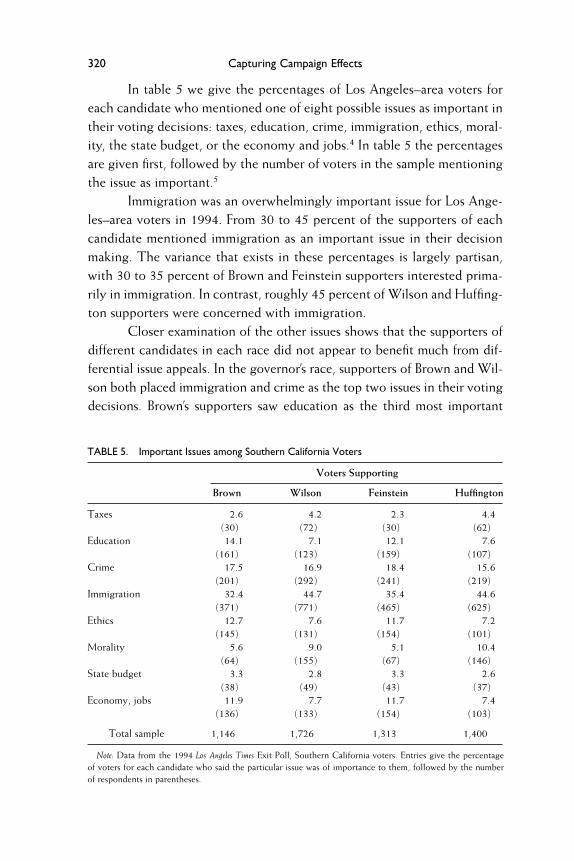
In table 5 we give the percentages of Los Angeles–area voters foreach candidate who mentioned one of eight possible issues as important intheir voting decisions: taxes, education, crime, immigration, ethics, moral-ity, the state budget, or the economy and jobs.4 In table 5 the percentagesare given Arst, followed by the number of voters in the sample mentioningthe issue as important.5

Immigration was an overwhelmingly important issue for Los Ange-les–area voters in 1994. From 30 to 45 percent of the supporters of eachcandidate mentioned immigration as an important issue in their decisionmaking. The variance that exists in these percentages is largely partisan,with 30 to 35 percent of Brown and Feinstein supporters interested prima-rily in immigration. In contrast, roughly 45 percent of Wilson and HufAng-ton supporters were concerned with immigration.

Closer examination of the other issues shows that the supporters ofdifferent candidates in each race did not appear to beneAt much from dif-ferential issue appeals. In the governor’s race, supporters of Brown and Wil-son both placed immigration and crime as the top two issues in their votingdecisions. Brown’s supporters saw education as the third most important


TABLE 5. Important Issues among Southern California Voters

Voters Supporting

Brown Wilson Feinstein Huffington

Taxes 2.6 4.2 2.3 4.4(30) (72) (30) (62)

Education 14.1 7.1 12.1 7.6(161) (123) (159) (107)

Crime 17.5 16.9 18.4 15.6(201) (292) (241) (219)

Immigration 32.4 44.7 35.4 44.6(371) (771) (465) (625)

Ethics 12.7 7.6 11.7 7.2(145) (131) (154) (101)

Morality 5.6 9.0 5.1 10.4(64) (155) (67) (146)

State budget 3.3 2.8 3.3 2.6(38) (49) (43) (37)

Economy, jobs 11.9 7.7 11.7 7.4(136) (133) (154) (103)

Total sample 1,146 1,726 1,313 1,400

Note: Data from the 1994 Los Angeles Times Exit Poll, Southern California voters. Entries give the percentageof voters for each candidate who said the particular issue was of importance to them, followed by the numberof respondents in parentheses.

issue, closely followed by personal ethics and the economy. Wilson’s sup-porters, though, saw four issues in a rough tie for third place in importance:education, ethics, morality, and the economy. Notice also that more Brownsupporters saw crime as an important issue than Wilson supporters, andWilson tapped the crime hot button, whereas Brown did not.

A similar pattern holds in the Senate race. Again, immigration andcrime are the two most important issues for both Feinstein and HufAngtonsupporters. Feinstein’s supporters show the same issue ordering as Brown’s(education followed by ethics and the economy). HufAngton’s supportershave the same issue rankings as Wilson: morality, education, the economy,and ethics in a four-way tie).

While interesting, the simple results in table 5 give only the bivari-ate relationships between issue preferences and candidate support. To ex-amine the multivariate impact of issue preferences on candidate choice, weestimated three bivariate probit models. In each set of bivariate probitmodels, one dependent variable is coded 1 for a Republican vote and 0 fora Democratic vote in the gubernatorial race. The second dependent vari-able is coded likewise for the Senate race. We use bivariate probit in thiscase, as there is strong reason to believe that a voter’s choice in one racemight impact his or her choice in the other race and that this mutual de-pendence of voter choice might be motivated by the information he or shereceives from the candidate’s advertisement strategies. The bivariate probitmodel controls for this type of mutual dependence by estimating the cor-relation between the error term of each vote choice model, and it willallow us to examine the joint impact of issue importance on voting in eachrace simultaneously.

We include seven dummy variables for issue preferences in each bi-variate probit model, with each being coded 1 if the voter said that a partic-ular issue was important to them and 0 otherwise (the economy and jobs isthe excluded category, so all the coefAcients we estimate for issue prefer-ences in our probit models are interpreted as the effect of mentioning theparticular issue relative to mentioning the economy and jobs as an importantissue). As control variables, we include dummy variables for gender (1 forwomen, 0 for men) and minority status (1 for ethnic minorities, 0 fornon–ethnic minorities). There also are controls for pocketbook voting, partyidentiAcation, and ideology (personal Anances is coded with the high cate-gory representing voters who felt they were better off, the middle categorythe same, and the lower category worse off; partisanship with Democratic


identiAcation is coded with the low category, independence the middle, andRepublican identiAcation the high category; ideology is coded as liberalswith the low category and conservatives the high category, with moderatesin the middle category).

To examine how the different issues impacted voter decision mak-ing, we estimate three different bivariate probit models. All of the estima-tion results are presented in table 6. The Arst two columns of table 6 givethe bivariate probit results for the full sample of Southern California vot-ers, with one column presenting estimation results for gubernatorial votingand the other, Senate voting. The next four columns of table 6 provide two


TABLE 6. Probit Estimates

All SC Voters High Education Low EducationIndependentVariables Governor Senate Governor Senate Governor Senate

Constant �2.8* �2.9* �2.8* �3.1* �2.8* �2.6*.16 .16 .21 .21 .26 .24

Taxes .38* .36* .36* .44* .39* .23*.08 .08 .11 .11 .13 .12

Education �.32* �.05 �.44* �.06 �.11 �.04.09 .09 .11 .12 .14 .14

Crime .28* .02 .34* .06 .19* �.09.07 .07 .10 .09 .11 .10

Immigration .42* .35* .36* .44* .52* .20*.07 .07 .10 .10 .12 .11

Ethics .06 .06 .13 .23* �.02 �.14.11 .11 .14 .14 .18 .18

Morality .39* .51* .56* .65* .23 .35*.14 .14 .19 .18 .23 .22

State budget .06 .08 �.17 �.18 .39* .43*.18 .18 .24 .24 .28 .28

Gender .08 �.08 .05 �.09 .10 �.11.07 .06 .09 .09 .10 .01

Minority �.58* �.26* �.28* �.31* �.93* �.34*.09 .09 .13 .15 .13 .13

Personal �.05 �.14* �.10* �.12* .05 �.14*Finances .04 .04 .06 .05 .07 .07Party ID .89* .89* .94* .88* .86* .91*

.04 .04 .06 .06 .06 .06Ideology .51* .50* .51* .53* .51* .49*

.05 .05 .07 .07 .08 .08 .68* .71* .64*

.03 .04 .05Sample 2,581 1,437 1,123Log-likelihood ratio �1,803.6 �971.0 �787.5

Note: Entries are bivariate probit estimates from the 1994 Los Angeles Times Exit Poll.*Statistically significant at the p � .05 level, one-tailed tests

reestimations of this full bivariate probit model, Arst for high educationvoters and then for low education voters. These latter two sets of bivariateprobit results examine how media awareness inBuences the impact of can-didate issue advertisements on voter decision making.6

In the full sample of Southern California voters, the coefAcient es-timates of primary interest are those for the issue preference variables. It isimportant to note that a number of these variables have statistically signi-Acant estimates. In the governor’s race, taxes, education, crime, immigra-tion, and morality all have statistically signiAcant effects. The positivesigns on these four parameters indicate that voters who thought that taxes,crime, immigration, or morality were important issues were signiAcantlymore likely to vote for Wilson, while voters who prioritized educationwere more likely to vote for Brown. Next, in the third column of table 6are the results for Senate voting. Here, only three issue priorities have sta-tistically signiAcant effects on voting: taxes, immigration, and morality.

Do the results in table 3 demonstrate that candidate television ad-vertisements had an impact on candidate choice? Perhaps. Recall table 1,where we gave the relative frequencies of candidate television advertise-ments on these same issues. We found that in the governor’s race the can-didates advertised mainly on crime, immigration, education, and the econ-omy. In table 6 we present results that indicate that all of these issues wereimportant to voters in this race. Furthermore, by stressing immigration,crime, and the economy, Wilson increased his support. Brown, on theother hand, obtained support for her emphasis on education.

In contrast, the candidates in the Senate race advertised much morefrequently on issues of personal ethics and morality; they also advertised,but to a much lesser extent, about crime and immigration. Again, the Sen-ate results in table 6 show that immigration appears to have been an im-portant determinant of Senate voting. Also, morality was a strong inBuenceon Senate voting.

The next issue we addressed was that of media awareness and its im-pact on voters’ decisions. Ideally, we would use responses to questions di-rectly measuring the voters’ media exposure or campaign interest.7 How-ever, as the Los Angeles Times Exit Poll did not include questions of this sort,we instead used information gathered on the education level of the votersas a proxy for media exposure (Alvarez 1997). Thus, we stratiAed thesample into low and high education groups, with the basic criterion of clas-siAcation being whether the voter had completed a college education. We


estimated the bivariate probit models separately for each of the twogroups, and the results are presented in the last four columns of table 6.

In table 6 four issues—taxes, crime, immigration, and the statebudget—are statistically signiAcant in gubernatorial voting for low educa-tion respondents. Of these, immigration seems to have the strongest in-Buence on the likelihood of voting for Wilson, with taxes and crime wellbehind in estimated impact. But the high education voters, who we assumeare more exposed to campaign advertisements, used more issue informa-tion in their voting: taxes, education, crime, immigration, and morality allare statistically signiAcant predictors of their gubernatorial votes. For thehigh education voters, morality and education seem to have the strongesteffects, with crime, taxes, and immigration slightly behind. The main dif-ference between high and low education voters, then, lies in the emphasisthat high education voters placed on education and morality and that loweducation voters placed on immigration. Since one of these issues (edu-cation) was emphasized in Brown’s television advertisements, we concludethat exposure to television advertisements appears to enhance the impor-tance of the issues stressed in the campaign in voter decisions.

The same analysis is repeated for Senate voting in table 6. Taxes, im-migration, morality, and the state budget were again the important issues tolow education Senate voters. But for high education Senate voters, who weargue are more exposed to candidate television advertisements, taxes, immi-gration, ethics, and morality are statistically signiAcant. Thus, as in thegubernatorial race, candidate television advertisements reached more ex-posed individuals. Notice that there are two differences between high andlow education Senate voters: for high education voters both ethics andmorality were important components of their decisions and the state budgetwas not. Given the intense focus in the Senate race on both ethics andmorality, and the understandable lack of focus on the state budgetary out-look, we conclude that more exposed voters may have been affected by theadvertisements in the Senate race.

Another way to examine the impact of these different issues on voterchoice and to see the degree of inBuence by candidate advertising focus isto use the bivariate probit results to make speciAc predictions about voterdecisions under different “counterfactual” conditions. Using the bivariateprobit results in table 6, we produce predicted probabilities that a hypothet-ical modal voter would cast ballots for Wilson and HufAngton (a straightRepublican ticket), for Brown and HufAngton (a divided ticket), for Wilson


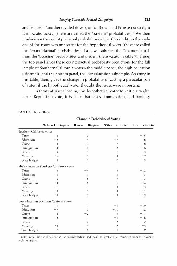
and Feinstein (another divided ticket), or for Brown and Feinsten (a straightDemocratic ticket) (these are called the “baseline” probabilities).8 We thenproduce another set of predicted probabilities under the condition that onlyone of the issues was important for the hypothetical voter (these are calledthe “counterfactual” probabilities). Last, we subtract the “counterfactual”from the “baseline” probabilities and present these values in table 7. There,the top panel gives these counterfactual probability predictions for the fullsample of Southern California voters; the middle panel, the high educationsubsample; and the bottom panel, the low education subsample. An entry inthis table, then, gives the change in probability of casting a particular pairof votes, if the hypothetical voter thought the issues were important.

In terms of issues leading this hypothetical voter to cast a straight-ticket Republican vote, it is clear that taxes, immigration, and morality


TABLE 7. Issue Effects

Change in Probability of Voting

Wilson-Huffington Brown-Huffington Wilson-Feinstein Brown-Feinstein

Southern California voterTaxes 14 0 1 �15Education �5 4 �7 8Crime 4 �2 7 �8Immigration 14 0 2 �16Ethics 2 1 0 3Morality 18 2 �3 �17State budget 3 1 0 �3

High education Southern California voterTaxes 13 �4 3 �12Education �3 1 �1 3Crime 2 �5 7 �3Immigration 14 �6 6 �14Ethics �3 �3 3 3Morality 12 1 �3 �11State budget 17 �1 �2 �15

Low education Southern California voterTaxes 15 1 �1 �16Education �7 5 �10 12Crime 4 �2 9 �11Immigration 15 1 �1 �16Ethics 7 2 �2 �7Morality 24 1 �2 �23State budget �6 0 �1 7

Note: Entries are the difference in the “counterfactual” and “baseline” probabilities computed from the bivariateprobit estimates.

were winning issues for Wilson and HufAngton. As shown in the Arst col-umn of table 7, the salience of these issues for this hypothetical Los Ange-les voter would lead her to be fourteen (taxes), fourteen (immigration), oreighteen (morality) points more likely to vote for Wilson and HufAngtonon the basis of each issue alone. Returning to table 1, taxes and immigra-tion were issues that were presented exclusively by Wilson and HufAngtonin their television advertising.

As for issues leading to a straight-ticket Democratic vote, it is clearby table 7 that only one issue worked for the Democrats—education. Inthe full sample results, if the hypothetical voter thought education was animportant issue, she would be eight points more likely to vote for Brownand Feinstein. However, only Brown focused advertising on this issue.

For the Democrats, especially Dianne Feinstein, the issue of per-sonal morality was clearly a loser. In the full sample results in the top panelof table 7, we see that, if the hypothetical voter thought this was an impor-tant issue, she would be seventeen points less likely to vote for Brown andFeinstein. This was the issue, though, that formed much of the basis forFeinstein’s attack advertising against HufAngton, and from our results, itdoes not appear that Feinstein was successful in gaining voter supportthrough her attacks on HufAngton’s morality. Finally, there is one issue thatseemed to lead this hypothetical voter to split her ticket: the issue of crime.In the full sample results, a voter who felt crime was an important issue waseight points less likely to cast a straight Democratic ticket but was sevenpoints more likely to cast a vote for Pete Wilson and Dianne Feinstein. Intable 1 we showed that crime formed much of the basis of Wilson’s adver-tising, and it was one of the issues that both HufAngton and Feinstein usedin their advertising. The results in table 6 show that crime was an issue onwhich Pete Wilson and Dianne Feinstein were viewed as successful.

Our third expectation was that issues, in general, ought to have agreater impact in voting for governor than for Senator, since the governor’srace generally was more issue focused than the Senate race (which wasmuch more character oriented). We used the bivariate probit results fromtable 6 to test this hypothesis. We reestimated the same probit models,after excluding the issue variables in one of the vote choice equations. Thisproduced a statistical test for the joint signiAcance of issues in these votingmodels.9 The relevant �2 statistics for testing the joint effects of issues ineach model are presented in table 8.

In table 8 there is clear support for this expectation. First, notice


that the �2 statistic for issue voting in the governor’s race is much greaterthan the same �2 for issue voting in the Senate race. Further, the �2 statis-tics for issue voting in the governor’s race in both the high and low educa-tion subsamples are much greater than in the Senate models. Both of theseresults provide strong support for the claim that with more issue discussionin the governor’s race issues became more important to voters’ decisions inthat race. We also see in table 8 another important result: issues had thelargest effect for highly educated voters in the governor’s race. This veri-Aes both our second and third expectations, since the voters most exposedto the media were the most reliant on issue voting in the race dominatedby discussion of issues.10

Advertisements and Candidate Evaluations

In this section we explore the hypothesis that candidate television adver-tisements change the general opinions voters have about the candidates orpersuade people to vote for one candidate over the other. To test this, weuse survey data from a different source: the Field Polls conducted duringthe general election among California voters. We use the July 12–17, Sep-tember 13–18, and October 21–30 Field Polls.11

These three Field Polls are useful since each poll asked registeredvoters two important types of questions. The Arst were the general “posi-tive-negative” evaluations of each candidate. The second were trial heats ineach race, in which voters were asked to state which candidate they wouldvote for were the election to be held on the day of the interview.

In table 9 we give the “positive-negative” evaluations of each candi-date in these three Field Polls. We present the percentages giving each eval-uative response, and we calculate the net change over the general electionperiod in the last column. Recall that Wilson ran mostly positive advertise-ments about himself; the negative attack advertisements he ran were mainlyabout Brown’s stand on issues, three to four weeks before the election.


TABLE 8. Tests for Issue Voting

Race Full Sample Low Education High Education

Governor 92.1* 33.4* 62.1*Senate 48.7* 12.8 45.1*

Note: Entries are �2 statistics testing for the importance of issue voting in the probit results. Each test hasseven degrees of freedom, and statistically significant entries are denoted by *.

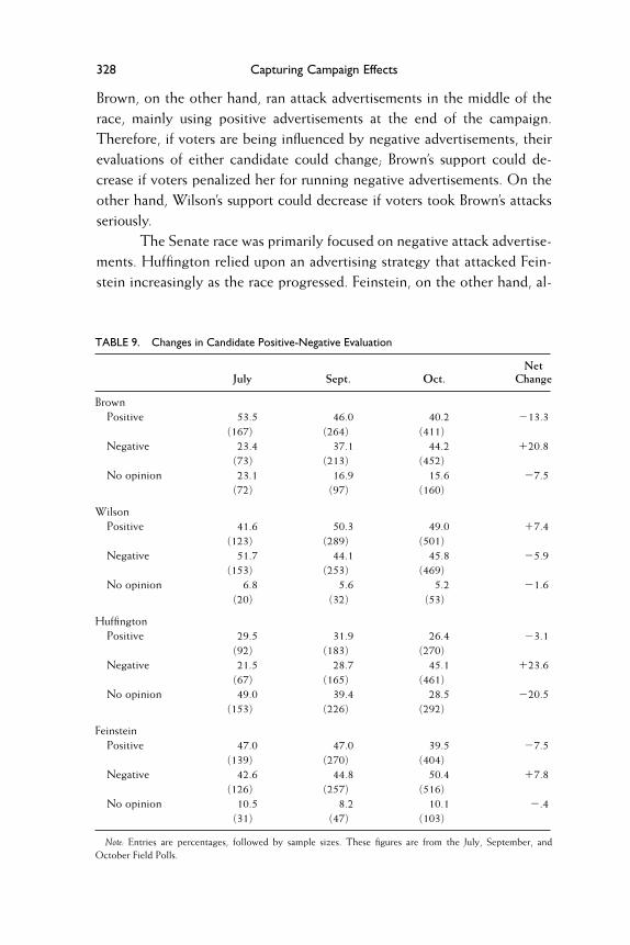
Brown, on the other hand, ran attack advertisements in the middle of therace, mainly using positive advertisements at the end of the campaign.Therefore, if voters are being inBuenced by negative advertisements, theirevaluations of either candidate could change; Brown’s support could de-crease if voters penalized her for running negative advertisements. On theother hand, Wilson’s support could decrease if voters took Brown’s attacksseriously.

The Senate race was primarily focused on negative attack advertise-ments. HufAngton relied upon an advertising strategy that attacked Fein-stein increasingly as the race progressed. Feinstein, on the other hand, al-


TABLE 9. Changes in Candidate Positive-Negative Evaluation

NetJuly Sept. Oct. Change

BrownPositive 53.5 46.0 40.2 �13.3

(167) (264) (411)Negative 23.4 37.1 44.2 �20.8

(73) (213) (452)No opinion 23.1 16.9 15.6 �7.5

(72) (97) (160)

WilsonPositive 41.6 50.3 49.0 �7.4

(123) (289) (501)Negative 51.7 44.1 45.8 �5.9

(153) (253) (469)No opinion 6.8 5.6 5.2 �1.6

(20) (32) (53)

HuffingtonPositive 29.5 31.9 26.4 �3.1

(92) (183) (270)Negative 21.5 28.7 45.1 �23.6

(67) (165) (461)No opinion 49.0 39.4 28.5 �20.5

(153) (226) (292)

FeinsteinPositive 47.0 47.0 39.5 �7.5

(139) (270) (404)Negative 42.6 44.8 50.4 �7.8

(126) (257) (516)No opinion 10.5 8.2 10.1 �.4

(31) (47) (103)

Note: Entries are percentages, followed by sample sizes. These figures are from the July, September, andOctober Field Polls.

most exclusively relied upon attack advertisements. Therefore, one shouldexpect either of two possible dynamics in candidate evaluations: if nega-tive advertisements against the opponent are successful, negative evalu-ations should rise and positive evaluations should fall during the cam-paigns; the other possible effect is that negative advertisements “backAre”and negatively inBuence the evaluations of their sponsor. Given that bothcandidates used mainly negative advertisements, it will be difAcult to dis-cern between these two explanations.

In table 9 it appears that Wilson might have won the battle of theairwaves. During the general election, his positive evaluations increased by7 percent, his negative evaluations decreased by 6 percent, and the num-ber of people who have no opinion about his evaluation decreased slightly.By running mainly positive television advertisements about his own posi-tions and a few advertisements against Brown’s character at the end of thecampaign, Wilson seems to have led California voters toward more posi-tive (and less negative) evaluations of himself. Kathleen Brown, on theother hand, seems to have been the loser of the television advertisingbattle. Her positive evaluations fell considerably (13 percent), while hernegative evaluations rose greatly (by 21 percent). The fact that Brown’spositive evaluations fell and her negative evaluations rose indicates that hermainly positive message did not resonate with the electorate—or that itdid not get through to most voters.

To some extent, the same dynamic was observed in the Senate race.There, HufAngton’s positive evaluations fell slightly during the generalelection (3 percent), while his negative evaluations skyrocketed upward(24 percent). Notice for HufAngton, though, that the percentages of vot-ers who said they had no opinion about HufAngton fell considerably, from49 percent in July to 29 percent in October. This indicates that HufAng-ton was doing what challengers need to do—inform voters about theircandidacy. The unfortunate problem for HufAngton, though, was that, asthe campaign wore on, the drop in the percentage of voters who had noopinion about HufAngton was matched by the rise in the percentage ofvoters who had a negative evaluation of HufAngton.

Feinstein’s positive evaluations fell during the general election by 7percent, and her negative evaluations rose by 8 percent. Feinstein began thegeneral election with relatively high positive and negative evaluations (47percent and 43 percent, respectively). The campaign produced a slight dropin her positive evaluations and a slight rise in her negative evaluations. The


evidence from the Senate race, then, indicates that attack advertising in-Buenced the electorate in this election: As the intensity of attack advertise-ments increased, so did the negative evaluations of both candidates. Attackswere focused on the opponent’s character, similar to Brown’s attack adver-tisements. HufAngton, who aired considerably fewer attack advertisementsin the Anal weeks of the campaign than did Feinstein, seems to have beenthe loser in terms of voter evaluations.

The next pressing question concerns whether these changes in can-didate evaluations, which seem to track the television advertising strategiesof the candidates, inBuenced the basic preferences of voters in each race.In table 10 we present the changes in the percentages of voters who sup-ported the candidates in each race, in the same three Field Polls.

In the top panel of table 10 we present the results for the governor’srace. For Wilson, the changes appear dramatic. In July, about 39 percent ofCalifornia voters supported Wilson, which put him slightly behind Brownin the polls. But by October, almost 51 percent of voters said they pre-ferred Wilson, which gave him a lead in the polls of almost 10 percent,with only days to go before the election. This is a 12 percent increase inWilson support, coming mainly from the ranks of undecided voters. Thisindicates that Wilson’s positive advertisements—and the rise in his positiveevaluations—led to a large change in support for Wilson among Califor-nia’s most important voters: those who were undecided in the early monthsof the general election.


TABLE 10. Changes in Candidate Projected Votes

NetJuly Sept. Oct. Change

Brown 42.7 41.0 41.5 �1.2(265) (233) (388)

Wilson 38.5 48.8 50.5 �12.0(241) (277) (473)

Undecided 16.3 10.2 8.0 �8.3(102) (58) (75)

Huffington 39.0 44.5 41.0 �2.0(237) (252) (366)

Feinstein 44.4 40.6 46.5 �2.1(270) (230) (415)

Undecided 16.6 14.8 12.5 �4.1(101) (84) (112)

Note: Entries are percentages, followed by sample sizes. These figures are from the July, September, andOctober Field Polls.

In the lower panel of table 10 we give the same Agures for the Sen-ate race. The dynamics of candidate preference in this race are remarkable.In July, Feinstein had a 5.5 percent lead over HufAngton. Though Feinsteinfell behind HufAngton in September, she regained her 5.5 percent leadover her opponent by October. The slight increase in support for bothcandidates (roughly 2 percent over the general election) was obtainedfrom the ranks of the undecided voters, who split evenly for the two can-didates by October. This shows that, while the attack strategies used byboth candidates led to increased negative evaluations for the two candi-dates, the attack advertisements allowed Feinstein to keep HufAngton’s ad-vances in the polls to a minimum.

Conclusions

In this essay we have undertaken a careful case study of the television ad-vertisement strategies used by four separate campaigns in two statewideraces in California during the 1994 election. We have shown that in thisparticular set of campaigns there was dramatic heterogeneity in candidatetelevision advertisements, which we argue was due to different strategiesemployed by each candidate.

We also showed that the advertising strategies used by the candidatesdid inBuence the target audience. We presented data from both exit pollstaken on Election Day and from telephone polls taken throughout the gen-eral election period, which demonstrated the effect of campaigns on which is-sues mattered in candidate choices on Election Day and also showed the cor-relation of attack advertisement strategies and changes in general candidateevaluations. Finally, we presented evidence that advertisements did shapechanges in candidate preferences over the course of the general election.

Obviously we examined only four individual campaigns, in a partic-ular election year, occurring in a state in which candidates for statewideofAce are forced to rely heavily on television advertising. The fact that thisis a case study does limit the generalizability of the results here regardingcandidate television strategies and voter responses to those strategies. Butwe feel that this study does show that more work of this sort is desperatelyneeded.

Political campaigns in general, and television advertisement cam-paigns in particular, are not well understood in the academic political sci-ence literature. In fact, there is still some debate as to whether campaigns


“matter”—whether they inBuence the electorate in substantial ways (e.g.,Finkel 1993). Unfortunately, there have been few systematic studies ofcampaigns, and those that have been undertaken have been primarily con-cerned with presidential election campaigns. While presidential electionsare important to study, presidential elections have characteristics that makethem poor cases for our exclusive analytical focus. First, there is little vari-ation in the media coverage and intensity of presidential campaigns, atleast in recent years (Alvarez 1997; Graber 1983; Patterson 1980). With-out much variation across campaigns in coverage or intensity, it is difAcultto imagine how presidential elections can shed much light on these impor-tant campaign variables. Second, the sample of presidential elections isquite limited. Obviously presidential elections occur every four years, so inthe time for which we have reliable survey data, we only have a handful orso of cases of presidential elections.

In this essay we have focused on subnational races—in particular,statewide races for ofAce. Moving our analytic focus from the nationallevel to the state level should serve to enhance our ability to understandhow campaigns operate and what effects they have on the electorate. Ineach four-year presidential election cycle, there are roughly one thousandraces in congressional and gubernatorial elections, with dramatic variationin campaign intensity, resource utilization, television advertising, mediacoverage, and the number of candidate debates and appearances. It is clearthat this is a laboratory well suited to the study of political campaigns inAmerica that is underutilized.

Therefore, by studying how four different candidates in two differ-ent races in the same election year tried to target voters in the same geo-graphic area, we can get a clear sense of how voters respond to campaignmessages. Thus, when one campaign focuses on a particular issue but theother campaigns do not, and we And that voters become concerned aboutthat particular issue over the election cycle, we may provide clear evidenceof the effect of a campaign message. To this effect, it is clear that statewidecampaigns provide a much better laboratory for studying campaigns thando presidential campaigns.

NOTESWe thank the John Randolph Haynes and Dora Haynes Foundation for its supportof this research project and the John M. Olin Foundation for its support of our re-search through a Faculty Fellowship. Kin Chang assisted with the collection of the


data presented in this essay, and Reginald Roberts assisted with early analysis.Henry Brady and Richard Johnston provided invaluable comments on an earlierdraft.

1. In the governor’s race, Pete Wilson was the Republican incumbent andKathleen Brown was his Democratic challenger. In the U.S. Senate race, DianneFeinstein was the Democratic incumbent and Michael HufAngton was her Repub-lican challenger.

2. See Bartels and Vavreck 2000; and Jamieson, Waldman, and Sher 1998 forfurther explanation of these three categories.

3. Advertising focus and tone are often closely interrelated. Most advertise-ments targeting the opposing candidate are attacking or contrasting, while most ad-vertisements about the candidate himself or herself are positive or contrasting. In theanalysis that follows we concentrate on the tone of advertising in these campaigns.

4. The focus on only Los Angeles or Southern California voters in the surveydata is to match up as closely as possible the survey data with the television adver-tisement data. It is obviously possible that the candidates ran different types or dif-ferent mixes of advertisements in different parts of the state; this would only com-plicate and obfuscate the analysis of the television and survey data.

5. The question posed by the survey was, “Which issues—if any—were mostimportant to you in deciding how to vote today? (Check up to two boxes).” The is-sues, in the order they appeared on the survey form, were taxes, education, crime,immigration, ethics, morality, business, environment, health care, state budget,economy, and none. The issues of business, environment, and health care were notused in this analysis since less than 1 percent of voters thought they were importantand since they were not issues that the candidates discussed in their advertisements.

6. The interested reader will note that all of the estimates for each of the threebivariate probit models are statistically signiAcant, indicating that indeed there isa substantial amount of unmeasured and correlated factors driving voters to makejoint decisions in these two races.

7. Druckman (2002), for instance, designed an exit poll that asked respon-dents to which local newspapers they subscribed and how often they read the frontpage of their subscriptions. This, of course, is a superior way to measure exposureto news coverage of campaign messages, but it does not measure exposure and/orattention to actual campaign advertisements themselves.

8. The baseline probabilities for the full sample are .27 (Wilson-HufAngton),.07 (Brown-HufAngton), .20 (Wilson-Feinstein), and .46 (Brown-Feinstein); for thehigh education sample, .25 (Wilson-HufAngton), .05 (Brown-HufAngton), .22(Wilson-Brown), and .48 (Brown-Feinstein); and for the low education sample, .37(Wilson-HufAngton), .14 (Brown-HufAngton), .14 (Wilson-Feinstein), and .35(Brown-Feinstein).

9. This is the standard test for joint signiAcance in discrete choice models,where twice the difference between the log-likelihoods of the restricted and unre-stricted models has a �2 distribution, with the degrees of freedom being equal tothe number of restrictions being tested.

10. Recall that higher education was used as a proxy for media awareness.11. The Field Institute conducts the California Poll at various times throughout

each year. They are telephone surveys of the adult population of California.


REFERENCESAllsop, D., and H. F. Weisberg. 1988. “Measuring Change in Party IdentiAcation

in Election Campaigns.” American Journal of Political Science 32:996–1017.Alvarez, R. M. 1997. Information and Elections. Ann Arbor: University of Michigan

Press.Ansolabehere, S., and S. Iyengar. 1995. Going Negative. New York: Free Press.Ansolabehere, S., S. Iyengar, A. Simon, and N. Valentino. 1994. “Does Attack Ad-

vertising Demobilize the Electorate?” American Political Science Review 88:829–38. Bartels, L. M., and L. Vavreck. 2000. Campaign Reform: Insights and Evidence. Ann

Arbor: University of Michigan Press.Basil, M., C. Schooler, and B. Reeves. 1991. “Positive and Negative Advertising:

Effectiveness of Ads and Perceptions of Candidates.” In Television and Political Advertising—Volume I: Psychological Processes, Communication and Society, ed. F. Biocca.Hillsdale, NJ: Lawrence Erlbaum.

Berelson, B., P. F. Lazarsfeld, and W. McPhee. 1954. Voting: A Study of Opinion For-mation in a Presidential Campaign. Chicago: University of Chicago Press.

Brians, C. L., and M. P. Wattenberg. 1996. “Campaign Issue Knowledge andSalience: Comparing Reception from TV Commercials, TV News and Newspa-pers.” American Journal of Political Science 40:145–71.

Campbell, A., P. E. Converse, W. E. Miller, and D. E. Stokes. 1960. The AmericanVoter. New York: Wiley.

Combs, J. E. 1979. “Political Advertising as a Popular Myth-Making Form.” Journalof American Culture 2:331–40.

Dalager, Jon K. 1996. “Voters, Issues, and Elections: Are the Candidates’ MessagesGetting Through?” Journal of Politics 58:486–515.

Druckman, J. 2002. “Priming the Vote: Campaign Effects in a U.S. Senate Elec-tion.” Working Paper, University of Minnesota, Minneapolis.

Faber, R. J., and M. C. Storey. 1984. “Recall of Information from Political Adver-tisements.” Journal of Advertising 13:39–44.

Ferejohn, J. A., and R. G. Noll. 1978. “Uncertainty and the Formal Theory ofPolitical Campaigns.” American Political Science Review 72:492–505.

Finkel, S. E. 1993. “Reexamining the ‘Minimal Effects’ Model in Recent Presiden-tial Campaigns.” Journal of Politics 55:1–21.

Fiorina, M. P. 1981. Retrospective Voting in American National Elections. New Haven: YaleUniversity Press.

Freedman, P., and K. Goldstein. 1999. “Measuring Media Exposure and the Effectsof Negative Campaign Ads.” American Journal of Political Science 43:1189–208.

Fridkin Kahn, K., and P. J. Kenney. 2002. “The Slant of the News: How EditorialEndorsements InBuence Campaign Coverage and Citizens’ Views of Candi-dates.” American Political Science Review 96:381–94.

Garramone, G. M. 1984. “Voter Responses to Negative Political Ads.” JournalismQuarterly 61:250–59.

———. 1985. “Effects of Negative Political Advertising: The Roles of Sponsor andRebuttal.” Journal of Broadcasting and Electronic Media 29:147–59.

Garramone, G. M., C. K. Atkin, B. E. Pinkleton, and R. T. Cole. 1990. “Effects ofNegative Advertising on the Political Process.” Journal of Broadcasting and ElectronicMedia 34:299–311.


Glazer, A. 1990. “Voting and Campaigning under Incomplete Information.” Euro-pean Journal of Political Economy 6:89–98.

Graber, Doris A. 1983. “Hoopla and Horse-Race in 1980 Campaign Coverage: ACloser Look.” In Mass Media and Elections: International Research Perspectives, ed. W.Schulz and K. Schoenbach. Munich, Germany: Oelschlaeger.

Guskind, R., and J. Hagstrom. 1988. “In the Gutter.” National Journal 20:2782–90.Jacobson, G. C. 1992. The Politics of Congressional Elections. New York: Harper Collins.Jamieson, K. H., P. Waldman, and S. Sher. 1998. “Eliminate the Negative? DeAn-

ing and ReAning Categories of Analysis for Political Advertisements.” Paper pre-sented at the Conference on Political Advertising in Election Campaigns, Wash-ington, DC.

Johnson-Cartee, Karen S., and Gary A. Copeland. 1991. Negative Political Advertising:Coming of Age. Hillsdale, NJ: Erlbaum.

Just, M., A. Crigler, and L. Wallach. 1990. “Thirty Seconds or Thirty Minutes:What Viewers Learn from Spot Advertisements and Candidate Debates.” Journalof Communication 40:120–33.

Kern, M. 1989. 30-Second Politics: Political Advertising in the Eighties. New York: Praeger.Lau R., and G. Pomper. 2002. “Effectiveness of Negative Campaigning in U.S. Sen-

ate Elections.” American Journal of Political Science 46:47–66.Lazarsfeld, P., B. Berelson, and H. Gaudet. 1944. The People’s Choice. New York: Co-

lumbia University Press.MacKuen, M. B., R. S. Erikson, and J. Stimson. 1992. “Peasants or Bankers? The

American Electorate and the U.S. Economy.” American Political Science Review86:597–611.

Merritt, S. 1984. “Political Advertising: Some Empirical Findings.” Journal of Adver-tising 13:27–38.

Patterson, T. C. 1980. The Mass Media Election. New York: Praeger.Patterson, T. C., and R. D. McClure. 1976. The Unseeing Eye. New York: Putnam.Roddy, B. L., and G. M. Garramone. 1988. “Appeals and Strategies of Negative Po-

litical Advertising.” Journal of Broadcasting and Electronic Media 32:415–27.Sellers, Patrick J. 1998. “Strategy and Background in Congressional Campaigns.”

American Political Science Review 92:159–71.Skarpedas, S., and B. Grofman. 1995. “Modeling Negative Campaigning.” American

Political Science Review 89:49–60.Surlin, S. H., and T. F. Gordon. 1977. “How Values Affect Attitudes toward Direct

Reference Political Advertising.” Journalism Quarterly 54:89–98.Wattenberg, M. P. 1991. The Rise of Candidate-Centered Politics. Cambridge, MA: Har-

vard University Press.West, D. M. 1993. Air Wars. Washington, DC: Congressional Quarterly.


studying statewide political campaigns · studying the advertising strategies of statewide...

Documents