STRUCTURE-AWARE SURFACERECONSTRUCTION WITH SPARSE

MOVING LEAST SQUARES

Alexander Lelidis

Bachelor ThesisAugust 2015

Supervisors:Prof. Dr. Markus Gross (ETH)

Prof. Dr. Marc Alexa (TU)Dr. Cengiz Öztireli (ETH)

Declaration of originality The signed declaration of originality is a component of every semester paper, Bachelor’s thesis, Master’s thesis and any other degree paper undertaken during the course of studies, including the respective electronic versions.

Lecturers may also require a declaration of originality for other written papers compiled for their courses.

__________________________________________________________________________ I hereby confirm that I am the sole author of the written work here enclosed and that I have compiled it in my own words. Parts excepted are corrections of form and content by the supervisor.

Title of work (in block letters):

Authored by (in block letters):

For papers written by groups the names of all authors are required.

Name(s): First name(s):

With my signature I confirm that

− I have committed none of the forms of plagiarism described in the ‘Citation etiquette’ information sheet.

− I have documented all methods, data and processes truthfully.

− I have not manipulated any data.

− I have mentioned all persons who were significant facilitators of the work.

I am aware that the work may be screened electronically for plagiarism. Place, date Signature(s)

For papers written by groups the names of all authors are

required. Their signatures collectively guarantee the entire content of the written paper.

Abstract

Surface reconstruction from scanned data is still an important task in computer graphics. It isthe only way to get a discrete representation of real world models. In this thesis, we proposea reconstruction framework, which combines successful methods from different fields of com-puter science and can easily be extended. Our approach is based on the assumption, that mostreal world surfaces can be characterized by a few features. This fact leads us to compressivesensing and dictionary learning. Our method extends the classical moving least squares tech-nique with a learned dictionary and a sparse solving process. This reformulation gives us inreturn the fast reconstruction due to the local nature of MLS, but also does not lose the globalview of the data thanks to the learned dictionary. Our technique is capable of reconstructingundersampled and noisy models in a state-of-the-art run time. Extensive experiments show ourprogress and document our way from the one to the three dimensional case. Additionally, weimplement a few established reconstruction methods in our framework, which allows us a livecomparison of the different results and shows that our method is able to keep up with them.

iii

Summary

This bachelor thesis engages the problem of surface reconstruction from oriented 3D points.We propose a new technique that combines methods from the field of compressive sensing anddictionary learning. The local nature of the moving least squares, enables fast surface recon-struction, but still keeps the global geometry in context with the precomputed dictionary. In thisthesis we review the roots of surface reconstruction, the state-of-the-art methods and discusstheir advantages and disadvantages. In terms of compressive sensing we discuss the differentdefinitions of sparsity and their mathematical models. We also shortly look into dictionarylearning and its usage in surface reconstruction. After a related work review we explain thetheoretical idea of our algorithm and take a deeper look into moving least squares, K-SVD andsolving a least squares system with a sparse constraint. In our experiments we try to prove thatthe theory works and create tests for the 1D and 2D case. We analyze the run time and the errorof different L1 norm base solvers. Finally, we summarize the results of our contribution.

v

Zusammenfassung

Diese Bachelorarbeit beschäftigt sich mit dem Problem der Oberflächenrekonstrution von ori-entierten 3D Punkten. Es wird eine neue Technik vorgestellt, welche Methoden aus dem Bere-ich "compressive sensing" (komprimiertes Abtasten) und "dictionary learning" (maschinellesLernen) kombiniert. Aufgrund der lokalen Definition von "moving least squares" (bewegtekleinste Fehlerquadrate) wird eine schnelle Oberflächenrekonstruktion ermöglicht, wobei derglobale Blick auf die Geometrie aufgrund des vorberechneten Wörterbuchs nicht vernachlässigtwird. In dieser Abschlussarbeit werden die Grundlagen der Oberflächenrekonstruktion aufgear-beitet und die Vor- und Nachteile von aktuell angewandten Methoden diskutiert. Im Bereich"compressive sensing" werden verschiedene Definitionen von "sparsity" (Seltenheit) und derenmathematische Modelle betrachtet. Es werden Methoden zum Erlernen eines Wörterbuchs erar-beitet und ihre Anwendung im Feld der Oberflächenrekonstrution diskutiert. Nach der Revisionder zusammenhängenden Methoden und Algorithmen, wird das theoretische Fundament derneuen Methode geschaffen. Dabei ist eine detaillierte Auseinandersetzung mit dem movingleast squares und dem K-SVD Algorithmus notwendig. Zusätzlich erfolgt eine Betrachtung derLösung von linearen Gleichungssystemen mit einer Sparsity Einschränkung. In anschließen-den Experimenten wird versucht, die Theorie zu überprüfen. Es werden verschiede Tests fürzunächst den eindimensionalen und darauffolgend den zweidimensionalen Fall erstellt. DieLaufzeit und die Rekonstrutionsfehler von verschiedenen L1-norm basierenden Lösern werdenanalysiert. Abschließend werden die Ergebnisse zusammengefasst.

vii

Contents

List of Figures xi

List of Tables xiii

1. Introduction 1

2. Related Work 32.1. Surface reconstruction . . . . . . . . . . . . . . . . . . . . . . . . . . . . . . 3

2.1.1. Direct methods . . . . . . . . . . . . . . . . . . . . . . . . . . . . . . 42.1.2. Indirect methods . . . . . . . . . . . . . . . . . . . . . . . . . . . . . 4

2.2. Sparse signal reconstruction . . . . . . . . . . . . . . . . . . . . . . . . . . . 62.3. Dictionary learning . . . . . . . . . . . . . . . . . . . . . . . . . . . . . . . . 8

3. Reconstruction model 93.1. Problem definition . . . . . . . . . . . . . . . . . . . . . . . . . . . . . . . . 93.2. Moving least squares . . . . . . . . . . . . . . . . . . . . . . . . . . . . . . . 9

3.2.1. Least squares . . . . . . . . . . . . . . . . . . . . . . . . . . . . . . . 103.2.2. Weighted Least squares . . . . . . . . . . . . . . . . . . . . . . . . . . 103.2.3. Moving weighted least squares . . . . . . . . . . . . . . . . . . . . . . 113.2.4. MLS for surface reconstruction . . . . . . . . . . . . . . . . . . . . . 11

3.3. Compressed sensing and surface reconstruction . . . . . . . . . . . . . . . . . 123.3.1. Sparse minimization with equality constraints . . . . . . . . . . . . . . 123.3.2. Least squares minimization with sparsity constraints . . . . . . . . . . 143.3.3. Sparse regularized least squares . . . . . . . . . . . . . . . . . . . . . 143.3.4. Sparse moving least squares . . . . . . . . . . . . . . . . . . . . . . . 14

ix

Contents

3.4. Designing the basis . . . . . . . . . . . . . . . . . . . . . . . . . . . . . . . . 153.4.1. Gaussian height field . . . . . . . . . . . . . . . . . . . . . . . . . . . 153.4.2. K-SVD . . . . . . . . . . . . . . . . . . . . . . . . . . . . . . . . . . 17

4. Experiments 194.1. 1D case . . . . . . . . . . . . . . . . . . . . . . . . . . . . . . . . . . . . . . 19

4.1.1. Compress sensing experiments . . . . . . . . . . . . . . . . . . . . . . 194.1.2. Sparse function reconstruction with Gaussian RBF . . . . . . . . . . . 21

4.2. 2D case . . . . . . . . . . . . . . . . . . . . . . . . . . . . . . . . . . . . . . 254.2.1. Testing on a function . . . . . . . . . . . . . . . . . . . . . . . . . . . 254.2.2. Reconstruction with implicit function . . . . . . . . . . . . . . . . . . 284.2.3. Results . . . . . . . . . . . . . . . . . . . . . . . . . . . . . . . . . . 284.2.4. Testing on a height field . . . . . . . . . . . . . . . . . . . . . . . . . 284.2.5. Adding the dictionary . . . . . . . . . . . . . . . . . . . . . . . . . . 30

4.3. 3D case . . . . . . . . . . . . . . . . . . . . . . . . . . . . . . . . . . . . . . 324.3.1. 3D Moving least squares . . . . . . . . . . . . . . . . . . . . . . . . . 334.3.2. Optimization . . . . . . . . . . . . . . . . . . . . . . . . . . . . . . . 334.3.3. Gaussian height field . . . . . . . . . . . . . . . . . . . . . . . . . . . 354.3.4. Adding the dictionary . . . . . . . . . . . . . . . . . . . . . . . . . . 364.3.5. Creating the data . . . . . . . . . . . . . . . . . . . . . . . . . . . . . 374.3.6. Results . . . . . . . . . . . . . . . . . . . . . . . . . . . . . . . . . . 38

5. Conclusion and Outlook 41

A. Appendix 43A.1. Detailed run time information of different sparse solvers. . . . . . . . . . . . . 43A.2. Detailed run time information for the reconstruction . . . . . . . . . . . . . . . 51

Bibliography 55

x

List of Figures

1.1. Michelangelo David scanning . . . . . . . . . . . . . . . . . . . . . . . . . . 2

3.1. Marching cubes configurations . . . . . . . . . . . . . . . . . . . . . . . . . . 123.2. Distribution of the Gaussian centers . . . . . . . . . . . . . . . . . . . . . . . 16

4.1. 256 coefficients of the original signal. . . . . . . . . . . . . . . . . . . . . . . 204.2. Least squares reconstruction (red). . . . . . . . . . . . . . . . . . . . . . . . . 204.3. 1D sparse reconstruction . . . . . . . . . . . . . . . . . . . . . . . . . . . . . 214.4. 1D reconstruction . . . . . . . . . . . . . . . . . . . . . . . . . . . . . . . . . 224.5. Least squares compared to sparse coefficients . . . . . . . . . . . . . . . . . . 224.6. 1D coefficient comparison . . . . . . . . . . . . . . . . . . . . . . . . . . . . 234.7. Varying lambda in 1D . . . . . . . . . . . . . . . . . . . . . . . . . . . . . . . 244.8. 1D noise . . . . . . . . . . . . . . . . . . . . . . . . . . . . . . . . . . . . . . 244.9. Testing the sigma parameter for the reconstruction . . . . . . . . . . . . . . . . 264.10. 2D function . . . . . . . . . . . . . . . . . . . . . . . . . . . . . . . . . . . . 264.11. Local coordinate systems of the 2D function . . . . . . . . . . . . . . . . . . . 274.12. local reconstruction . . . . . . . . . . . . . . . . . . . . . . . . . . . . . . . . 274.13. 2D function implicit reconstruction . . . . . . . . . . . . . . . . . . . . . . . . 284.14. Problems of 2d function implicit reconstruction . . . . . . . . . . . . . . . . . 294.15. 2D function implicit reconstruction with different solver . . . . . . . . . . . . 294.16. 1D dictionary usage . . . . . . . . . . . . . . . . . . . . . . . . . . . . . . . . 314.17. Implicit reconstruction results . . . . . . . . . . . . . . . . . . . . . . . . . . 324.18. 3D input points . . . . . . . . . . . . . . . . . . . . . . . . . . . . . . . . . . 334.19. 3D marching cubes . . . . . . . . . . . . . . . . . . . . . . . . . . . . . . . . 344.20. Speed up . . . . . . . . . . . . . . . . . . . . . . . . . . . . . . . . . . . . . . 354.21. Gaussian height field reconstruction . . . . . . . . . . . . . . . . . . . . . . . 36

xi

List of Figures

4.22. Sampling and error scalar field . . . . . . . . . . . . . . . . . . . . . . . . . . 374.23. Error of the reconstruction with and without dictionary . . . . . . . . . . . . . 39

A.1. 1D sparse reconstruction . . . . . . . . . . . . . . . . . . . . . . . . . . . . . 45A.2. 1D reconstruction with different solvers . . . . . . . . . . . . . . . . . . . . . 46A.3. L1LS . . . . . . . . . . . . . . . . . . . . . . . . . . . . . . . . . . . . . . . 46A.4. Computing 2D data . . . . . . . . . . . . . . . . . . . . . . . . . . . . . . . . 47A.5. Reconstructing 2D data . . . . . . . . . . . . . . . . . . . . . . . . . . . . . . 48A.6. Height field reconstruction . . . . . . . . . . . . . . . . . . . . . . . . . . . . 49A.7. 3D reconstruction . . . . . . . . . . . . . . . . . . . . . . . . . . . . . . . . . 50A.8. 1D Dictionary convergence . . . . . . . . . . . . . . . . . . . . . . . . . . . . 50A.9. 3D Dictionary runtime . . . . . . . . . . . . . . . . . . . . . . . . . . . . . . 51A.10.3D reconstruction with dictionary . . . . . . . . . . . . . . . . . . . . . . . . 52A.11.original and reconstructed mesh . . . . . . . . . . . . . . . . . . . . . . . . . 53A.12.Dictionary eigenvalues . . . . . . . . . . . . . . . . . . . . . . . . . . . . . . 53A.13.Dictionary elements . . . . . . . . . . . . . . . . . . . . . . . . . . . . . . . . 54

xii

List of Tables

A.1. Detailed run time . . . . . . . . . . . . . . . . . . . . . . . . . . . . . . . . . 43A.2. Runtime for reconstruction . . . . . . . . . . . . . . . . . . . . . . . . . . . . 51

xiii

1Introduction

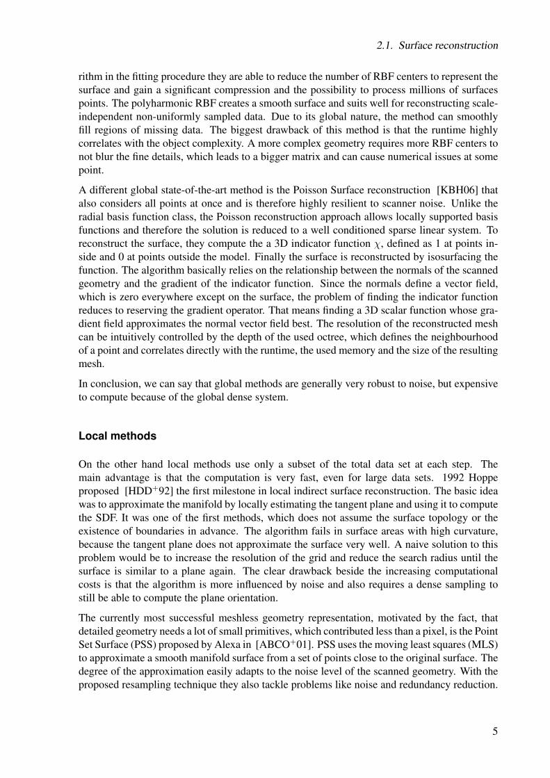
In the last years the amount and quality of 3D scanning devices have increased drastically.The devices are not anymore highly complicated scientific laboratory material, they are nowaffordable and easy to handle. A big step towards the user was the Kinect sensor, whose RGBDoutput could easily be used to create 3D point clouds. This example shows, how easy it is toget 3D scanned points. Of course there are many other devices, which all have their field ofapplication, depending on the scale, noise, scanning precision and scanning time. However,nearly all devices are facing the same problems. At first, there is the obvious trade-off betweenaccuracy and storage, which means that a detailed point cloud requires a large amount of points.A good example is the famous scanning project of Michelangelo’s David [Lev04], that required250 GB of storage. Also the trade-off between noise and scanning time is important. Most ofthe time we are not interested in the raw point set, but in the underlying surface. Since the early90s many robust surface reconstruction algorithms have been developed, which can handlescanning problems like noise, outliers and holes. It is useful to compute a 2D surface definedby a point could, that could be triangulated and used for rendering or animation. Reconstructinga surface from a raw point set is still an open challenge. The reasons behind this are various. Abig problem is the distinguishing between noise and sharp features of the surface. There is noclear mathematical way to separate noise from really sharp features, e.g. spikes or edges. Theusual way of handling noise is to average the neighboring points to smooth out the noise, whichworks really well, if the surface is very smooth. But in case of sharp features, they can easily getblurred out. Current methods rely on manually defining the areas with sharp features [GG07]or using precomputed dictionaries [XZZ+14a]. Since local approximation with moving leastsquares [Lev03] solves the problem efficiently, but gets easily confused by noise or outliersand loses the global view of the surface. Global methods using radial basis functions (RBF)are more robust, but don’t give a general solution. Reconstruction with RBF with a large inputpoint set requires solving a huge linear system. Regardless of the computational cost and runtime, the interpolation matrix could become ill conditioned and the solving could be unstable.

1

1. Introduction

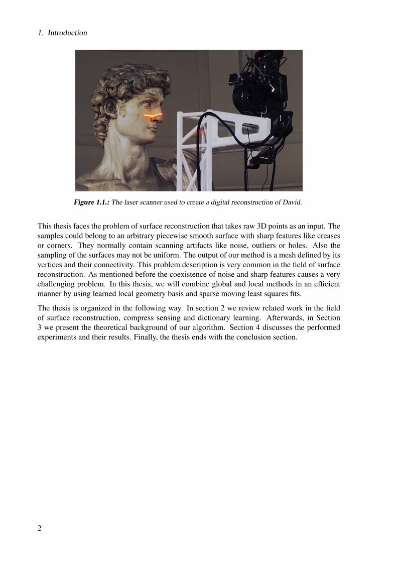
Figure 1.1.: The laser scanner used to create a digital reconstruction of David.

This thesis faces the problem of surface reconstruction that takes raw 3D points as an input. Thesamples could belong to an arbitrary piecewise smooth surface with sharp features like creasesor corners. They normally contain scanning artifacts like noise, outliers or holes. Also thesampling of the surfaces may not be uniform. The output of our method is a mesh defined by itsvertices and their connectivity. This problem description is very common in the field of surfacereconstruction. As mentioned before the coexistence of noise and sharp features causes a verychallenging problem. In this thesis, we will combine global and local methods in an efficientmanner by using learned local geometry basis and sparse moving least squares fits.

The thesis is organized in the following way. In section 2 we review related work in the fieldof surface reconstruction, compress sensing and dictionary learning. Afterwards, in Section3 we present the theoretical background of our algorithm. Section 4 discusses the performedexperiments and their results. Finally, the thesis ends with the conclusion section.

2

2Related Work

In the following section we give an overview of the relevant work, which we separate in 3parts. First, we take a look into surface reconstruction and discuss currently used algorithms,in terms of noise, sharp features and irregular sampling. In the second part we discuss sparsesignal reconstructions and review different mathematical solution approaches and their benefits.We also give an overview of the surface reconstruction algorithms, which use sparse norm forsurface reconstruction. Then, we shortly review methods from the field of dictionary learningand their application in the surface reconstruction.

2.1. Surface reconstruction

In the last 20 years a lot of research has be done in the domain of surface reconstruction fromscanned data. A lot of reconstruction algorithms have been proposed. However, nearly allexisting methods can be classified into direct and indirect methods, which both have differentbenefits and downsides. The direct methods on the one side may require denoising, because theydirectly operate on 3D scanned points, whose outliers can be very confusing. Also the selectionof a good subset of the scanned points, that gives a good representation of the surface, is achallenging task. Finally the resulting output needs to be triangulated to fit the given problemdescription.

On the other side indirect methods require the construction of an implicit function, which zeroset defines the surface. If we don’t get the surface normals from the scanning device, the algo-rithm needs to estimate those. Surface normals are very important for rendering algorithms andfor computing discrete differential mesh properties. Finally, we also need to run the marchingcubes algorithm [LC87] to obtain a triangular discrete mesh.

3

2. Related Work

2.1.1. Direct methods

Direct methods usually interpret a subset of scanned data points as vertices and try to link themdirectly to a graph, which represents the surface. It is very common to run the algorithm onlyon a subset of the input points, because otherwise resulting mesh would be very dense and notsmooth on continuous surface areas due to noise. A traditional algorithm for this purpose is theSpectral Surface Reconstruction [KSO04], where they perform Delaunay tetrahedralization,which is basically the 3D extension of Delaunay triangulation [CX04]. Afterwards they use aversion of spectral graph partitioning to decide whether each tetrahedron is inside or outside ofthe original surface. Because of the local inside-out decisions, which are based on the globalview of the model, this algorithm can handle a several amount of outliers and regions withno samples (holes). Still the spectral algorithm is not infallible, the biggest problem is that itproduces unwanted handles and has slow run time.

The more recent scale-space meshing method [DMSL11] proposes first to filter the raw inputdata based on the intrinsic heat equation, also called mean curvature motion (MCM) and thento interpolate the subset of the filtered points to reconstruct the surface. It is still likely that thismethod produces reconstruction artifacts like jaggy edges.

Another well established method [DG01] tackles the problem of detecting an undersampledsurface region. This scanning problem often appears on the boundary of a surface or a regionwith high curvature. The method uses this information to detect boundaries and sharp featureof the scanned object and uses them to reconstruct non smooth surfaces. The biggest drawbackis that the method makes some assumption about the distribution of the scanned points, whichare not necessarily fulfilled for every scanner.

A good overview of methods for surface reconstruction via Delaunay triangulation can be foundin [CG06].

In summary, we can say that direct methods are still very sensitive to noise. Additionally, thecomputation of the Delaunay tetrahedralization or the 3 dimensional Voronoi diagram is highlyexpensive in terms of memory and CPU time.

2.1.2. Indirect methods

Indirect methods, also called implicit surface reconstruction methods, construct an implicitfunction, typically a signed distance function (SDF). This function is positive on the outsideof the scanned object and negative on the inside. Indirect methods perform isosurfacing of thezero level set of that function to gain the surface of the scanned geometry. We can distinguishthe indirect methods in two main categories: local and global methods.

Global methods

Global methods for surface reconstruction consider all points at once and solve only one bigdense symmetric linear system. In 2001 J.C. Carr proposed a method [CBC+01] that recon-structs 3D Objects with polyharmonic radial basis functions (RBF). Through a greedy algo-

4

2.1. Surface reconstruction

rithm in the fitting procedure they are able to reduce the number of RBF centers to represent thesurface and gain a significant compression and the possibility to process millions of surfacespoints. The polyharmonic RBF creates a smooth surface and suits well for reconstructing scale-independent non-uniformly sampled data. Due to its global nature, the method can smoothlyfill regions of missing data. The biggest drawback of this method is that the runtime highlycorrelates with the object complexity. A more complex geometry requires more RBF centers tonot blur the fine details, which leads to a bigger matrix and can cause numerical issues at somepoint.

A different global state-of-the-art method is the Poisson Surface reconstruction [KBH06] thatalso considers all points at once and is therefore highly resilient to scanner noise. Unlike theradial basis function class, the Poisson reconstruction approach allows locally supported basisfunctions and therefore the solution is reduced to a well conditioned sparse linear system. Toreconstruct the surface, they compute the a 3D indicator function χ, defined as 1 at points in-side and 0 at points outside the model. Finally the surface is reconstructed by isosurfacing thefunction. The algorithm basically relies on the relationship between the normals of the scannedgeometry and the gradient of the indicator function. Since the normals define a vector field,which is zero everywhere except on the surface, the problem of finding the indicator functionreduces to reserving the gradient operator. That means finding a 3D scalar function whose gra-dient field approximates the normal vector field best. The resolution of the reconstructed meshcan be intuitively controlled by the depth of the used octree, which defines the neighbourhoodof a point and correlates directly with the runtime, the used memory and the size of the resultingmesh.

In conclusion, we can say that global methods are generally very robust to noise, but expensiveto compute because of the global dense system.

Local methods

On the other hand local methods use only a subset of the total data set at each step. Themain advantage is that the computation is very fast, even for large data sets. 1992 Hoppeproposed [HDD+92] the first milestone in local indirect surface reconstruction. The basic ideawas to approximate the manifold by locally estimating the tangent plane and using it to computethe SDF. It was one of the first methods, which does not assume the surface topology or theexistence of boundaries in advance. The algorithm fails in surface areas with high curvature,because the tangent plane does not approximate the surface very well. A naive solution to thisproblem would be to increase the resolution of the grid and reduce the search radius until thesurface is similar to a plane again. The clear drawback beside the increasing computationalcosts is that the algorithm is more influenced by noise and also requires a dense sampling tostill be able to compute the plane orientation.

The currently most successful meshless geometry representation, motivated by the fact, thatdetailed geometry needs a lot of small primitives, which contributed less than a pixel, is the PointSet Surface (PSS) proposed by Alexa in [ABCO+01]. PSS uses the moving least squares (MLS)to approximate a smooth manifold surface from a set of points close to the original surface. Thedegree of the approximation easily adapts to the noise level of the scanned geometry. With theproposed resampling technique they also tackle problems like noise and redundancy reduction.

5

2. Related Work

For rendering point set surfaces interactively they propose to use their upsampling method, ifthe point resolution is too small. The point resolution should be adapted with respect to thescreen space resolution. However, this method does not discretize the zero set of the implicitfunction to a mesh and keeps points, as the name suggests, as the surface primitives.

Another very popular method is the Algebraic Point Set Surfaces [GG07], that presents a newPoint Set Surface definition based on moving least squares fitting of algebraic spheres. TheAPSS method is much more robust in terms of low sampling rates or regions with high curva-ture. In consequence of the sphere fitting procedure, the method returns the mean curvature ofthe surface for free, which corresponds to the fitted sphere radius. In case of oriented pointsthe algorithm takes the normals into account for the minimization and punishes the gradientto the reconstructed function to match the direction of the normals. As an extension of theirmethod, they propose a way to handle sharp feature by classification of the two sides of an edgeperformed during the runtime by the user. The APSS algorithm uses only points from one classat a time to reconstruct the corresponding surface, which does not smooth the edges or cornersout and is able to reconstruct sharp feature.

Summarizing, we could say that local indirect surface reconstruction methods are much fasterthan the global ones. They do not suffer from numerical problems, but can easily get confusedby missing geometry if the local neighbourhood is too small.

2.2. Sparse signal reconstruction

In the last years compressed sensing (sparse signal reconstruction) has gained a lot of attractionin many fields like applied mathematics, computer science and signal processing. The maingoal of compressed sensing is to find a basis or dictionary in which group of signals can besparsely encoded and reconstructed. We consider a signal as sparse if most of the signal ele-ments are zero. The fraction between the zero and nonzero elements defines the sparsity of asignal. From a general viewpoint the reduction of dimensions leads to efficient modelling tech-niques and noise reduction. In 2004 the compressed sensing pioneer Emmanuel Candès proofedin [CRT05] that given the knowledge about the sparsity of the signal and the correspondingbasis, the data could be reconstructed with less samples than required by the Nyquist-sampling-theorem. That means underdetermined systems with normally infinite solutions can be solvedwith a constraint minimization (convex optimization) converging to the correct solution. Gen-erally speaking, compressed sensing takes advantage of the fact that the world is not totallyrandom. As a matter of fact many interesting signals are remarkably sparse if they are analyzedin the right domain. Finding the right domain (basis) for a given class of signals is one of themajor research topics in compressed sensing. In the next section we are going to discuss therelated work and algorithms for using a learned dictionary as a basis. However, assuming thatwe have the domain in which the observed signals are sparse, we still need to find a solutionfor the underdetermined system. The least-squares approach is to minimize the L2 norm of theenergy of the system

minx||Ax− y||22 (2.1)

6

2.2. Sparse signal reconstruction

where A stands for the basis of the sparse domain and y is the measured signal. This approachusually leads to poor reconstruction results, because the zero entries of the signal will get anonzero value which leads to the loss of sparsity. Also, in presence of noise the least squaresminimization leads to overfitting. To achieve better results and enforce sparsity, one couldminimize 2.1 with the L0 norm instead of the L2. The L0 norm counts the number of nonzero entries in a vector and is not a proper F-norm, because of its discontinuous definition.Solving this problem would return the optimal solution in terms of sparsity and reconstructionerror. But as proved by Dongdong et al. in [GJY10] finding the global minimum of theLp(0 ≤ p < 1) minimization is a strongly NP-hard problem. But again Candès and Rombergproved in [CR05a] that many L0 minimization problems can be solved by replacing the L0

norm with the L1 norm also known as Taxicab norm or Manhattan norm. The L1 norm isdefined as the sum of the absolute values of the entries of a vector

||x||1 =n∑i=0

|xi| (2.2)

Strictly speaking, it is equivalent, if the coefficient vector x is sparse enough, to solve the mucheasier L1 minimization instead of the NP-hard L0. In [SMW+07] Sharon et al. proposes analgorithm for determining the L1 - L0 equivalence for error correction and sparse representation.

Solving the a linear system with L1 norm can be expressed as a linear program or a basis pursuitdenoising.

However, compressed sensing has also found its way to the field of surface reconstruction.Similar to us, in 2010 Avron et al. assumed in [ASGCO10] that common objects, even geomet-rically complex ones, can typically be characterized by a rather small number of features. Thisrealization led them to the field of sparse signal reconstruction. They propose a global sparsemethod which uses the L1 norm and solves the problem in a two-step fashion. First they solvethe orientation under the assumption that a smooth surface has smooth varying normals. Thecomputed orientations are used to compute the positions. To achieve a lower sparsity than L1

sparsity they use the iterative reweighted version [CWB08].

minx||Wx||1 s.t. ||Ax− y||22 (2.3)

whereW is a diagonal weighting matrix. The basic idea is to solve the equation ( 2.3) iteratively.In the first iterationW can be represented as the identity matrix and in next iteration the weightswi are defined inversely proportional to the true signal magnitude. However, their global sparsemethod achieves reasonable reconstruction, with concentrated error at the corners or edges,because points lying directly on these spots have no clearly defined orientation. This problemleads to spikes sticking out of the model.

Recently, another two-step method which uses the reweighed L1 was published in 2014 by R.Wang in [WYL+14]. Their main focus lies in on decoupling noise and features of a givengeometry. In the first phase they approximate a base mesh with a global Laplacian denoisingscheme. They prove that if the number of samples tends to infinity, the base mesh converges tothe underlying surface with probability 1. In the second phase they rely on the discovery thatsharp features can be sparsely represented by a dictionary constructed by the pseudo inverse

7

2. Related Work

of the Laplacian matrix. Recovering of those features is done by a progressive reweighted L1

minimization. The results of the method are quite good, if it is applied to meshes, becausemeshes in contrast to point clouds contain the basic information of the surface topology.

2.3. Dictionary learning

Dictionary learning is one of the most studied fields in machine learning. Sparse dictionarylearning uses the coefficients form some signals in a given basis to compute a new dictionary Din which the signals can be represented sparsely. Learning a dictionary is an NP-Hard problem[Til14], which is even very hard to approximate. The most popular approximation algorithm isthe K-SVD algorithm, which we are also going to use.

Dictionary learning has been used in several fields of science. In computer graphics it is mostlyused in image compression or inpainting. Recently, dictionary learning has also found its wayto 3D geometry processing. In 2014 J. Digne proposed in [DCV14] method, which exploitsthe self-similarity of underlying shapes. The algorithm locally resamples the point cloud anduses the new samples, which they call centers, to compute a dictionary of the local height fielddiscrete cosine transform (DCT) coefficients. Finally, they use the dictionary and the centers tocompress the point cloud without losing important information.

Another method for robust surface reconstruction using a dictionary was proposed in 2014 in[XZZ+14b]. They use a dictionary consisting out of the vertices of the reconstructed triangularmesh and a sparse coding matrix, which defines the connectivity of the vertices. They minimizefor the optimal triangulation of the input data, while taking many factors into account. As acost function, they define the distance between the reconstructed mesh and the input point set.The results are quite good and outperform a few state-of-the-art methods, but their optimizationmodel is nonconvex, which means they can not guarantee convergence against a global min-imum. Also, in case of missing data the algorithm has problems to fill those, because of themissing samples in that region.

8

3Reconstruction model

In the following section we are going to describe our approach more in detail and explain theused mathematical models and their properties. We start with a basic surface reconstructionalgorithm and along the section extend it. We begin by clearly formulating the discussed prob-lem.

3.1. Problem definition

Our problem can be characterized as follows: Given a point set containing n oriented 3D pointsP = {p0, p1, · · · , pn}, where pi ∈ R3 with corresponding normals N = {n0, n1, · · · , nn} , ni ∈R3 and ||ni||2 = 1 sampled from a closed manifold surface S. We try to find a discrete mesh Mthat is defined as a set of vertices and faces M = {V,F}. The vertex set V = {v0, v1, · · · , vn}defines the position of the geometry in space. The face set for triangular meshes is defined asF = {f | (vi, vj, vk) = f ∧vi 6= vj ∧vj 6= vk∧vi 6= vk, vi, vj, vk ∈ V}. The reconstructed meshshould approximate the surface S so that the numerical and visual error is as small as possible.

3.2. Moving least squares

Since the whole algorithm will build on moving least squares, we will start with the basic defini-tion proposed in 1981 [LS81] for smoothing and interpolating data. At first a brief explanationof the least squares problem is given.

9

3. Reconstruction model

3.2.1. Least squares

The least squares method is a very common method to approximate the solution of overdeter-mined systems. The standard example is fitting a line in a point cloud. In a more abstract waythat means that we want to compute a global function f(x) from N points pi and their functionvalues yi that the least squares error between f(pi) and yi is as small as possible. Consequentlywe need to minimize the following statement

minf

N∑i=0

||f(pi)− yi||22 (3.1)

where f is the reconstructed function and d is the dimension of the domain, in which the func-tion is defined in. Since the function f consists not of arbitrary elements, but is defined withrespect to some basis we can write ( 3.1) as

minc∈Rd

N∑i=0

||b(pi) · c− yi||22 (3.2)

where b(pi) is the basis for the point pi and c is the unknown coefficient vector, we are trying tocompute.

Equation ( 3.2) can be solved analytically by computing the partial derivatives and setting themto zero. If we write ( 3.2) in matrix form we get

LSerror = minc∈Rd||B(p)c− y||22 (3.3)

where B is the basis matrix. Now we need to compute the gradient ∇LSerror and set it to zeroto find a minimum.

∇LSerror = cTBTBc− 2yT +Bc+ yTy!

= 0 (3.4)

Since the last term of the equation does not depend on c, we remove it. Finally we need to solve

c = (BTB)−1 −BTy (3.5)

This operation could be problematic, because the matrix BTB is not necessarily easy to invert.However, for a more detailed derivation, we refer to [Fed15].

3.2.2. Weighted Least squares

The problem of using a least squares fit is that all points pi get treated equally, which is notwhat is preferred, because points which are far away from the evaluation point x get the sameweight as points really close to it. To address the issue, we introduce a weighting function θ(d),depending on the Euclidean distance between x and pi.

minfx∈Rd

N∑i=0

θ(||x− pi||2)||fx(pi)− yi||22 (3.6)

10

3.2. Moving least squares

In matrix form we getWLSerror = min

c∈RdW (x, p)||B(p)c− y||22 (3.7)

where W (x, p) is a diagonal matrix containing the weights on the diagonal. Again we can solvethe function analytically.

c = (BTWB)−1 −BTWy (3.8)

Weighting function

The choice of the weighting function depends on the application. A standard weighting functionto gain smooth varying weights with local support is a Gaussian function.

θ(d) = e−d2

σ2

where the additional parameter σ controls the width of the weighting function.

Another weighting function is the tricube weight function defined as

θ(d) =

{(1− |d|3)3 if |d| < 1

0 else

that has a very compact support and is used in LOESS [Cle79].

3.2.3. Moving weighted least squares

The moving least squares (MLS) is basically a weighted least squares which gets moved overthe domain Rd. The MLS function only takes the points inside a given radius r into account,which is the reason for the local support and the efficient evaluation. This problem reduction ispossible, because the weighting function gives points further way than the radius a weight closeto zero and they become neglectable for the local result.

minfx∈Rd

k∑i=0

θ(||x− pi||2)||fx(pi)− yi||22 (3.9)

where k is the number of points inside the radius r. The reconstructed function is continuouslydifferentiable if and only if the weighting function θ is continuously differentiable [Lev98].

3.2.4. MLS for surface reconstruction

All the explained methods are widely used in computer science. To get back to surface recon-struction we are going to describe the work flow for reconstructing a surface using MLS. Sincewe work with computers we need to discretize the 3d domain. Usually the best way is to createa grid inside the bounding box defined by the sampled points. An advantage of this methodis that computed results could be directly used as an input for the marching cubes algorithm

11

3. Reconstruction model

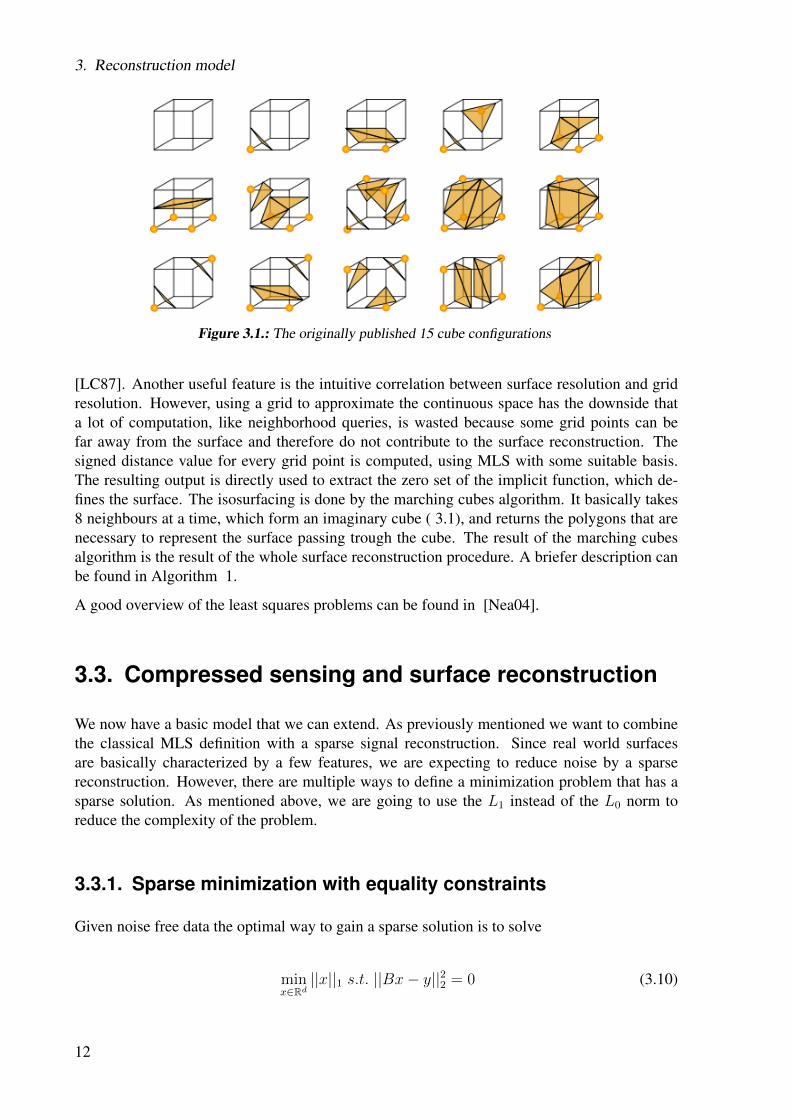
Figure 3.1.: The originally published 15 cube configurations

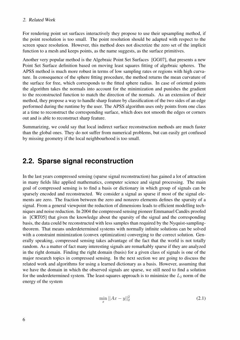
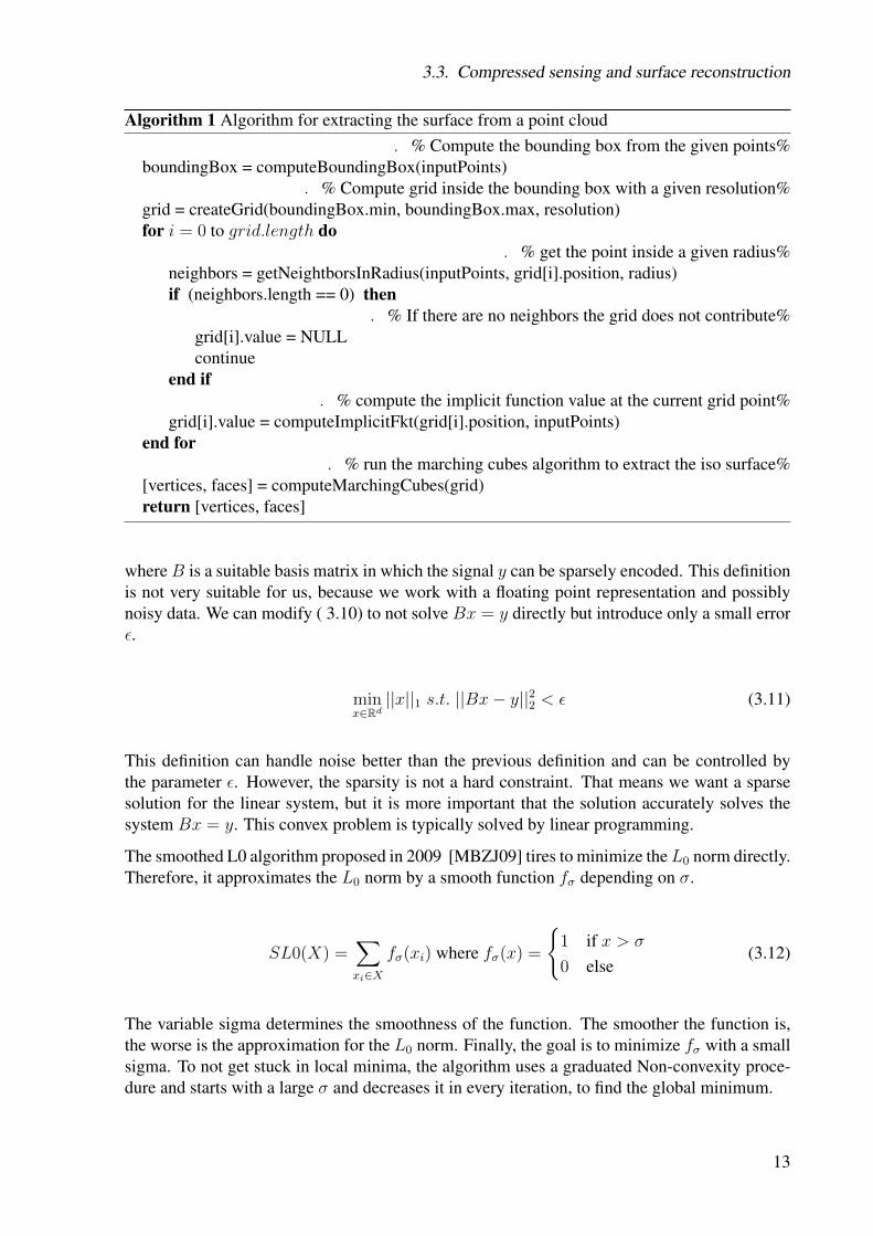
[LC87]. Another useful feature is the intuitive correlation between surface resolution and gridresolution. However, using a grid to approximate the continuous space has the downside thata lot of computation, like neighborhood queries, is wasted because some grid points can befar away from the surface and therefore do not contribute to the surface reconstruction. Thesigned distance value for every grid point is computed, using MLS with some suitable basis.The resulting output is directly used to extract the zero set of the implicit function, which de-fines the surface. The isosurfacing is done by the marching cubes algorithm. It basically takes8 neighbours at a time, which form an imaginary cube ( 3.1), and returns the polygons that arenecessary to represent the surface passing trough the cube. The result of the marching cubesalgorithm is the result of the whole surface reconstruction procedure. A briefer description canbe found in Algorithm 1.

A good overview of the least squares problems can be found in [Nea04].

3.3. Compressed sensing and surface reconstruction

We now have a basic model that we can extend. As previously mentioned we want to combinethe classical MLS definition with a sparse signal reconstruction. Since real world surfacesare basically characterized by a few features, we are expecting to reduce noise by a sparsereconstruction. However, there are multiple ways to define a minimization problem that has asparse solution. As mentioned above, we are going to use the L1 instead of the L0 norm toreduce the complexity of the problem.

3.3.1. Sparse minimization with equality constraints

Given noise free data the optimal way to gain a sparse solution is to solve

minx∈Rd||x||1 s.t. ||Bx− y||22 = 0 (3.10)

12

3.3. Compressed sensing and surface reconstruction

Algorithm 1 Algorithm for extracting the surface from a point cloud. % Compute the bounding box from the given points%

boundingBox = computeBoundingBox(inputPoints). % Compute grid inside the bounding box with a given resolution%

grid = createGrid(boundingBox.min, boundingBox.max, resolution)for i = 0 to grid.length do

. % get the point inside a given radius%neighbors = getNeightborsInRadius(inputPoints, grid[i].position, radius)if (neighbors.length == 0) then

. % If there are no neighbors the grid does not contribute%grid[i].value = NULLcontinue

end if. % compute the implicit function value at the current grid point%

grid[i].value = computeImplicitFkt(grid[i].position, inputPoints)end for

. % run the marching cubes algorithm to extract the iso surface%[vertices, faces] = computeMarchingCubes(grid)return [vertices, faces]

whereB is a suitable basis matrix in which the signal y can be sparsely encoded. This definitionis not very suitable for us, because we work with a floating point representation and possiblynoisy data. We can modify ( 3.10) to not solve Bx = y directly but introduce only a small errorε.

minx∈Rd||x||1 s.t. ||Bx− y||22 < ε (3.11)

This definition can handle noise better than the previous definition and can be controlled bythe parameter ε. However, the sparsity is not a hard constraint. That means we want a sparsesolution for the linear system, but it is more important that the solution accurately solves thesystem Bx = y. This convex problem is typically solved by linear programming.

The smoothed L0 algorithm proposed in 2009 [MBZJ09] tires to minimize theL0 norm directly.Therefore, it approximates the L0 norm by a smooth function fσ depending on σ.

SL0(X) =∑xi∈X

fσ(xi) where fσ(x) =

{1 if x > σ

0 else(3.12)

The variable sigma determines the smoothness of the function. The smoother the function is,the worse is the approximation for the L0 norm. Finally, the goal is to minimize fσ with a smallsigma. To not get stuck in local minima, the algorithm uses a graduated Non-convexity proce-dure and starts with a large σ and decreases it in every iteration, to find the global minimum.

13

3. Reconstruction model

3.3.2. Least squares minimization with sparsity constraints

Another slightly different formulation is

minx∈Rd||Bx− f ||22 s.t. ||x||1 < t (3.13)

where we minimize the least squares system with a hard sparsity constraint. This method ispreferred if the sparsity of the signal x is known. With the parameter t the sparsity of the signalis directly controlled.

This problems are typical solved by greedy algorithms like matching pursuit (MP) [MZ93].MP computes the best nonlinear approximation with respect to some basis or dictionary. Thisapproximation is stored in a sequence and repeated iteratively. A light extension is the orthogo-nal matching pursuit [TG07] which requires that after every step the extracted coefficients areprojected onto the selected basis. This procedure can create better results than the standard MPformulation, but the computation is also more expensive.

3.3.3. Sparse regularized least squares

Another possible way to formulate the problem as a L1 regularized least squares program:

minx∈Rd||Bx− f ||22 + λ||x||1 (3.14)

where λ is a weight to decide the importance of the sparsity of the solution. It is inverse corre-lated to the parameter t mentioned in formulation before. The class of the techniques is calledLASSO (Least Absolute Shrinkage and Selection Operator) and tries to combines L2 and L1

minimization, with the aim to get the advantages of both: A sparse solution with a small meansquared error. The problem could be remodeled as a convex quadratic problem and solve by aninterior point method.

A specialized interior point algorithm for solving large scale L1 regularized systems was pro-posed in [KKB07]. They use the preconditioned conjugate gradients method to compute thesearch direction for the next iteration step.

3.3.4. Sparse moving least squares

We remodel our MLS minimization to be sparse:

minc∈Rd

k∑i=0

θ(||x− pi||2)||b(pi) · c− yi||22 + λ||c||1 (3.15)

And in matrix notationminc∈Rd

W (x, p)||B(p)c− y||22 + λ||c||1 (3.16)

where we can regulate the sparsity of the solution with λ. To gain a sparse solution with a smallmean squared error the signal needs to be sparse in the the domain of the basis B. Assuming so,the parameter λ can be used to smooth out the surface and reduce noise. We propose to choosethe parameter λ accordingly to the expected noise level.

14

3.4. Designing the basis

3.4. Designing the basis

Finding the right basis or dictionary for a given class of signals is an open research problemin compressive sensing. In signal processing, wavelets often have been used as sparse basisfor oscillating signals or image compression. The basic idea is to express the data in a domain,where most of it can be represented as a sparse combination of the basis or atoms. If the numberof used basis tends to infinity the expressed signal will perfectly match the original one.

On the other hand, a learned dictionary also serves well as a domain, where the representationswould be sparse. A so called data-depended dictionary needs to be trained on data sets from thesame cluster, to compute the atoms of the dictionary. Finally, the signal from the same clustercan be represented as a linear combination of the atoms. With an increasing number of trainingdata and dictionary atoms the reconstruction error should converge to zero. If the dictionarywas trained on data with fine details like high frequencies, it is possible to reconstruct thosealso in case of under sampling. Furthermore, if the training signals where basically noise free,it is also possible to remove noise during the reconstruction. The dictionary training is an offlineprocess, which is very expensive in terms of memory usage and CPU time, but only needs to bedone once.

3.4.1. Gaussian height field

In our case we want to use a Gaussian height field (GHF) as basis. The GHF is defined by anumber of Gaussian centers and a corresponding σ value. But before we can define the GHFwe need to find a good reference coordinate system, which fits the local points well.

Local coordinates system

Since we iterate over the grid, representing the discrete approximation of the continuous 3Dspace, we only use the k points inside a sphere around the grid point x with radius r to estimatethe local frame. If the radius is small enough the given points form a proper height field. Toextract the height field we need to compute the principal directions of the points P inside thesphere. To extract those we first need to center the points by subtracting the mean point p fromevery point pi:

P = [p0 − p, p1 − p, · · · , pk − p] (3.17)

The next step is to compute the singular value decomposition of P ∈ R3×k.

UΣV T = SV D(P ) (3.18)

where the matrix U ∈ R3×3 contains the principal directions of P . To gain a height field weneed to express the points P in U , which is done by computing Plocal = UT P . Since we want tocenter our coordinate system at our evaluated grid point x, we need to transform x to the localcoordinate system xlocal = UT (x− p) and subtracted the resulting value from every point:

Plocalatx = [plocal0 − xlocal, plocal1 − xlocal, · · · , plocalk − xlocal]T (3.19)

The points in the matrix Plocalatx ∈ Rk×3 define now the height field.

15

3. Reconstruction model

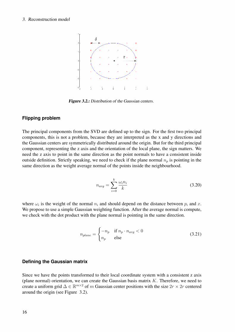
Figure 3.2.: Distribution of the Gaussian centers.

Flipping problem

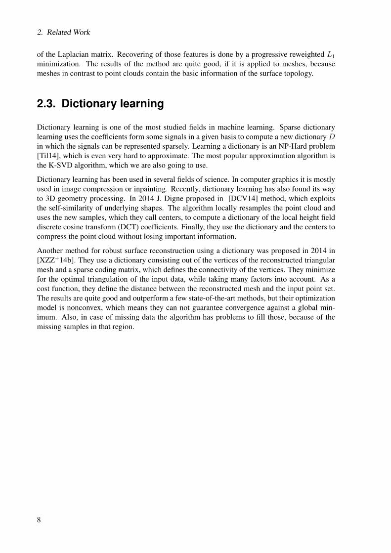
The principal components from the SVD are defined up to the sign. For the first two principalcomponents, this is not a problem, because they are interpreted as the x and y directions andthe Gaussian centers are symmetrically distributed around the origin. But for the third principalcomponent, representing the z axis and the orientation of the local plane, the sign matters. Weneed the z axis to point in the same direction as the point normals to have a consistent insideoutside definition. Strictly speaking, we need to check if the plane normal np is pointing in thesame direction as the weight average normal of the points inside the neighbourhood.

navg =k∑i=0

ωinik

(3.20)

where ωi is the weight of the normal ni and should depend on the distance between pi and x.We propose to use a simple Gaussian weighting function. After the average normal is compute,we check with the dot product with the plane normal is pointing in the same direction.

nplane =

{−np if np · navg < 0

np else(3.21)

Defining the Gaussian matrix

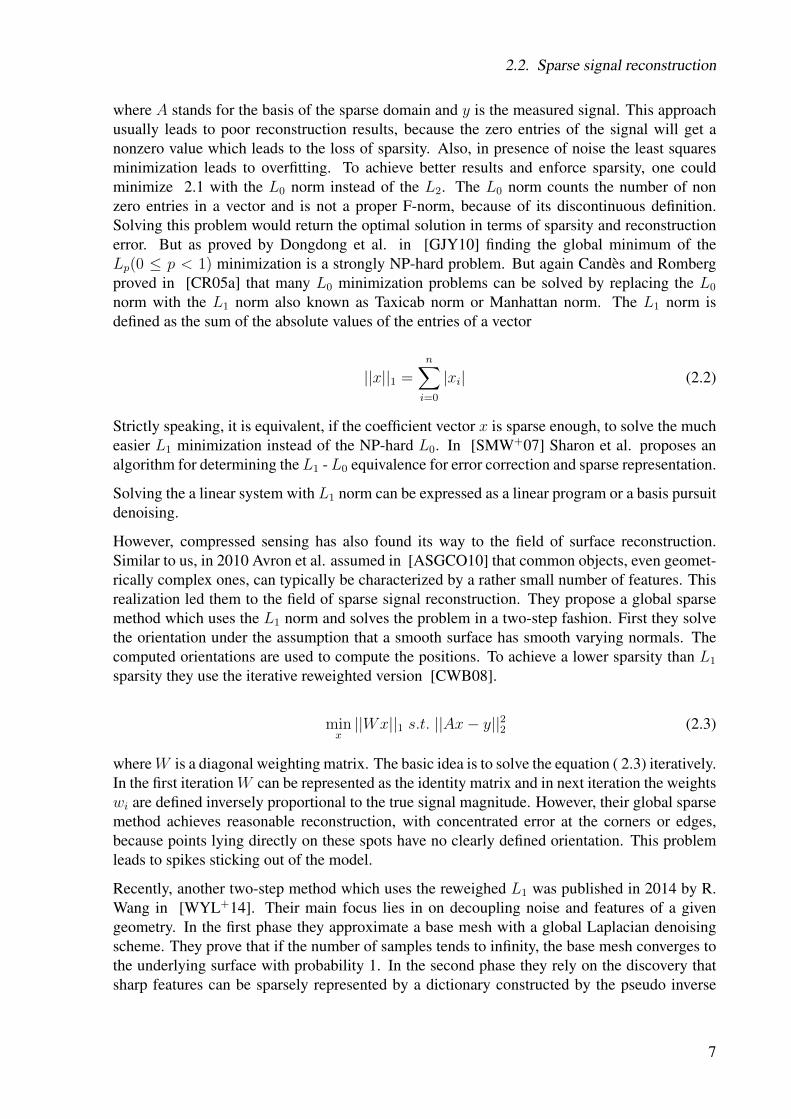
Since we have the points transformed to their local coordinate system with a consistent z axis(plane normal) orientation, we can create the Gaussian basis matrix K. Therefore, we need tocreate a uniform grid ∆ ∈ Rm×2 of m Gaussian center positions with the size 2r × 2r centeredaround the origin (see Figure 3.2).

16

3.4. Designing the basis

The Gaussian matrix K ∈ Rk×m is defined in the following way.

K =

e−||Φ0 −∆0||22

2σ2 e−||Φ0 −∆1||22

2σ2 . . . e−||Φ0 −∆m||22

2σ2

e−||Φ1 −∆0||22

2σ2 e−||Φ1 −∆1||22

2σ2 . . . e−||Φ1 −∆m||22

2σ2

...... . . . ...

e−||Φk −∆0||22

2σ2 e−||Φk −∆1||22

2σ2 . . . e−||Φk −∆m||22

2σ2

(3.22)

where Φ ∈ Rk×2 contains the xy coordinates of the transformed points Plocalatx. The parameterσ is defined depending on the radius r and the number of Gaussian centers along the firstdimension.

The final minimization problem we need to solve is:

minc∈Rm

W (x, p)||Km,r(p)c− f ||22 + λ||c||1 (3.23)

where f are the height values, which is equal to the third column of the transformed pointsPlocalatx,

Signed distance value

After solving the equation ( 3.23) we need to compute the implicit function value for the gridpoint x:

SDF (x) =

[e−||~0−∆0||22

2σ2 e−||~0−∆1||22

2σ2 . . . e−||~0−∆m||22

2σ2

]c (3.24)

We can use ~0 as position for x because we transform the local coordinate system to the gridpoint x.

3.4.2. K-SVD

Definition

For learning the dictionary we are going to use the K-SVD algorithm proposed in [AEB06].The algorithm creates a dictionary for discrete signal representation via sparse combinations ofthe dictionary atoms. The basic algorithm works in the following way.

Given a training matrix T ∈ Rd×n of signals, where d is the signal dimension and n is thenumber of samples. The goal of the algorithm is to compute an overcomplete dictionary out ofthe a atoms, where every signal can be represented as a sparse linear combination of the atoms

17

3. Reconstruction model

ai. That means every signal ti (column in the training matrix T ) can be reconstructed by solvingsparse minimization systems.

minxi∈Rd

||Dxi − ti||22 s.t. ||xi||0 < T0 (3.25)

where T0 defines the maximum number of non zero elements and thus determining the sparsityof the signal. We can write the previous equation in matrix form to solve the minimizationproblem for all signals simultaneously.

minX∈Rd×n

||DX − T ||2F ∀i ||xi||0 < T0 (3.26)

The K-SVD method solves the problem iteratively, by alternating between sparse coding of thetraining signals based on the current dictionary and a process of updating the dictionary atomsto better fit the data. In the sparse coding stage the algorithm uses a pursuit algorithm like Basispursuit or Orthogonal matching pursuit to compute the sparse coding. At the first iteration theinitial dictionary is created out of randomly selected training signals. In the updating state themethod updates every atom ai from the current dictionary. K-SVD determinates all trainingsignals which use ai in their reconstruction and compute the reconstruction error Ei on thedictionary D without ai. Afterwards Ei is decomposed in Ei = UΣV T . The first column inthe U matrix defines the new atom ai. The first column of the V matrix multiplied by the firstsingular value Σ0,0 defines the updated coefficients. The K-SVD pseudocode can be found inalgorithm 2.

Learning the dictionary

To learn the dictionary we iterate over the domain and use the coefficients from the reconstruc-tion of the signal as test data. This signal are the columns of the training matrix T . The size of Tdepends on the radius and the number of grid points. Finally we need to choose a compressionrate and a threshold for the sparse representation with the atoms. Usually the dictionary size isdisproportional to the threshold. That means if the dictionary size increases, we need less atomsto represent a signal precisely.

Usage in surface reconstruction

The final minimization system we work with is:

minc∈Rd

W (x, p)||K(p)Dc− y||22 + λ||c||1 (3.27)

where D defines the learned dictionary. We solve this problem with an alternating directionmethod of multipliers (ADMM), which is designed to solve convex optimization problems bybreaking them into smaller pieces. The algorithm was proposed by N. Parikh and S. Boyd in[BPC+11] and first defines a canonical problem form called graph form of the optimization.In the next step the method performs a graph projection splitting, a form of Douglas-Rachfordsplitting or the alternating direction method of multipliers, to solve graph form problems seri-ally. This algorithm is implemented in the POGS framework [Fou14] by Chris Fougner, whichwe are going to use to solve 3.27.

18

4Experiments

In the following section we are going to describe the experiments we carried out. At first weare only doing one dimensional tests, to get an overview of the behaviour of the solvers andthe reconstruction. After getting successful results we are moving on to the two dimensionalcase and trying to create the base for the three dimensional case. Finally, we use the gainedknowledge to implement a system for 3D reconstruction. In all dimensions we analyse the runtime and the resulting reconstruction error of different methods. For our experiments we usedthe numerical computing environment Matlab [MAT12] and the object oriented programminglanguage C++.

4.1. 1D case

4.1.1. Compress sensing experiments

Because our whole algorithm builds up on sparse solvers, we begin by testing different solvers.For that purpose we create a random Gaussian orthonormalized matrix A ∈ R128×256 withmean of 0 and standard deviation of 1, which we are going to use to create a measurementvector. For the measurement vector we create a 256 parameter long signal x0, which contains25 non zero elements see Figure 4.1. Together with matrix A we create a measurement vectory by multiplying A and x0

y = Ax0 (4.1)

The measurement vector y is used to reconstruct x0 with different solvers. After the reconstruc-

19

4. Experiments

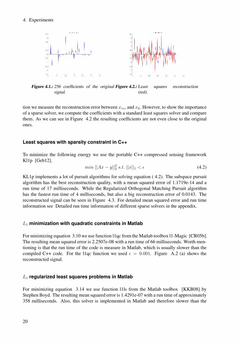
Figure 4.1.: 256 coefficients of the originalsignal.

Figure 4.2.: Least squares reconstruction(red).

tion we measure the reconstruction error between xrec and x0. However, to show the importanceof a sparse solver, we compute the coefficients with a standard least squares solver and comparethem. As we can see in Figure 4.2 the resulting coefficients are not even close to the originalones.

Least squares with sparsity constraint in C++

To minimize the following energy we use the portable C++ compressed sensing frameworkKl1p [Geb12].

min ||Ax− y||22 s.t. ||x||1 < ε (4.2)

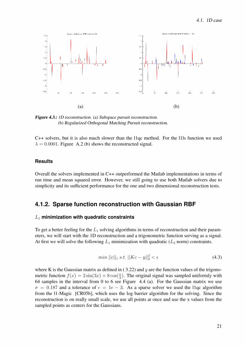
KL1p implements a lot of pursuit algorithms for solving equation ( 4.2). The subspace pursuitalgorithm has the best reconstruction quality, with a mean squared error of 1.1719e-14 and arun time of 17 milliseconds. While the Regularized Orthogonal Matching Pursuit algorithmhas the fastest run time of 4 milliseconds, but also a big reconstruction error of 0.0143. Thereconstructed signal can be seen in Figure 4.3. For detailed mean squared error and run timeinformation see Detailed run time information of different sparse solvers in the appendix.

L1 minimization with quadratic constraints in Matlab

For minimizing equation 3.10 we use function l1qc from the Matlab toolbox l1-Magic [CR05b].The resulting mean squared error is 2.2507e-08 with a run time of 66 milliseconds. Worth men-tioning is that the run time of the code is measure in Matlab, which is usually slower than thecompiled C++ code. For the l1qc function we used ε = 0.001. Figure A.2 (a) shows thereconstructed signal.

L1 regularized least squares problems in Matlab

For minimizing equation 3.14 we use function l1ls from the Matlab toolbox [KKB08] byStephen Boyd. The resulting mean squared error is 1.4291e-07 with a run time of approximately358 milliseconds. Also, this solver is implemented in Matlab and therefore slower than the

20

4.1. 1D case

(a) (b)

Figure 4.3.: 1D reconstruction. (a) Subspace pursuit reconstruction.(b) Regularized Orthogonal Matching Pursuit reconstruction.

C++ solvers, but it is also much slower than the l1qc method. For the l1ls function we usedλ = 0.0001. Figure A.2 (b) shows the reconstructed signal.

Results

Overall the solvers implemented in C++ outperformed the Matlab implementations in terms ofrun time and mean squared error. However, we still going to use both Matlab solvers due tosimplicity and its sufficient performance for the one and two dimensional reconstruction tests.

4.1.2. Sparse function reconstruction with Gaussian RBF

L1 minimization with quadratic constraints

To get a better feeling for the L1 solving algorithms in terms of reconstruction and their param-eters, we will start with the 1D reconstruction and a trigonometric function serving as a signal.At first we will solve the following L1 minimization with quadratic (L2 norm) constraints.

min ||c||1 s.t. ||Kc− y||22 < ε (4.3)

where K is the Gaussian matrix as defined in ( 3.22) and y are the function values of the trigono-metric function f(x) = 2 sin(3x) + 8 cos(x

2). The original signal was sampled uniformly with

64 samples in the interval from 0 to 6 see Figure 4.4 (a). For the Gaussian matrix we useσ = 0.187 and a tolerance of ε = 1e − 3. As a sparse solver we used the l1qc algorithmfrom the l1-Magic [CR05b], which uses the log barrier algorithm for the solving. Since thereconstruction is on really small scale, we use all points at once and use the x values from thesampled points as centers for the Gaussians.

21

4. Experiments

(a) (b)

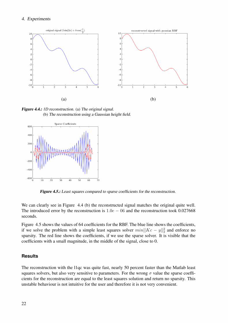
Figure 4.4.: 1D reconstruction. (a) The original signal.(b) The reconstruction using a Gaussian height field.

Figure 4.5.: Least squares compared to sparse coefficients for the reconstruction.

We can clearly see in Figure 4.4 (b) the reconstructed signal matches the original quite well.The introduced error by the reconstruction is 1.0e − 06 and the reconstruction took 0.027668seconds.

Figure 4.5 shows the values of 64 coefficients for the RBF. The blue line shows the coefficients,if we solve the problem with a simple least squares solver min||Kc − y||22 and enforce nosparsity. The red line shows the coefficients, if we use the sparse solver. It is visible that thecoefficients with a small magnitude, in the middle of the signal, close to 0.

Results

The reconstruction with the l1qc was quite fast, nearly 50 percent faster than the Matlab leastsquares solvers, but also very sensitive to parameters. For the wrong σ value the sparse coeffi-cients for the reconstruction are equal to the least squares solution and return no sparsity. Thisunstable behaviour is not intuitive for the user and therefore it is not very convenient.

22

4.1. 1D case

(a) (b)

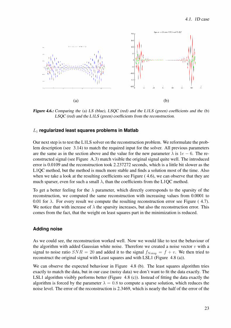
Figure 4.6.: Comparing the (a) LS (blue), LSQC (red) and the L1LS (green) coefficients and the (b)LSQC (red) and the L1LS (green) coefficients from the reconstruction.

L1 regularized least squares problems in Matlab

Our next step is to test the L1LS solver on the reconstruction problem. We reformulate the prob-lem description (see 3.14) to match the required input for the solver. All previous parametersare the same as in the section above and the value for the new parameter λ is 1e − 6. The re-constructed signal (see Figure A.3) match visible the original signal quite well. The introducederror is 0.0109 and the reconstruction took 2.237272 seconds, which is a little bit slower as theL1QC method, but the method is much more stable and finds a solution most of the time. Alsowhen we take a look at the resulting coefficients see Figure ( 4.6), we can observe that they aremuch sparser, even for such a small λ, than the coefficients from the L1QC method.

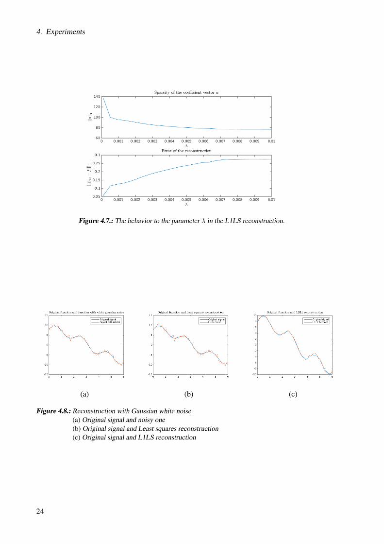
To get a better feeling for the λ parameter, which directly corresponds to the sparsity of thereconstruction, we computed the same reconstruction with increasing values from 0.0001 to0.01 for λ. For every result we compute the resulting reconstruction error see Figure ( 4.7).We notice that with increase of λ the sparsity increases, but also the reconstruction error. Thiscomes from the fact, that the weight on least squares part in the minimization is reduced.

Adding noise

As we could see, the reconstruction worked well. Now we would like to test the behaviour ofthe algorithm with added Gaussian white noise. Therefore we created a noise vector v with asignal to noise ratio SNR = 20 and added it to the signal fNoisy = f + v. We then tried toreconstruct the original signal with Least squares and with LSL1 (Figure 4.8 (a)).

We can observe the expected behaviour in Figure 4.8 (b). The least squares algorithm triesexactly to match the data, but in our case (noisy data) we don’t want to fit the data exactly. TheLSL1 algorithm visibly performs better (Figure 4.8 (c)). Instead of fitting the data exactly thealgorithm is forced by the parameter λ = 0.8 to compute a sparse solution, which reduces thenoise level. The error of the reconstruction is 2.3469, which is nearly the half of the error of the

23

4. Experiments

Figure 4.7.: The behavior to the parameter λ in the L1LS reconstruction.

(a) (b) (c)

Figure 4.8.: Reconstruction with Gaussian white noise.(a) Original signal and noisy one(b) Original signal and Least squares reconstruction(c) Original signal and L1LS reconstruction

24

4.2. 2D case

least squares reconstruction (4.5274).

Finding the optimal σ

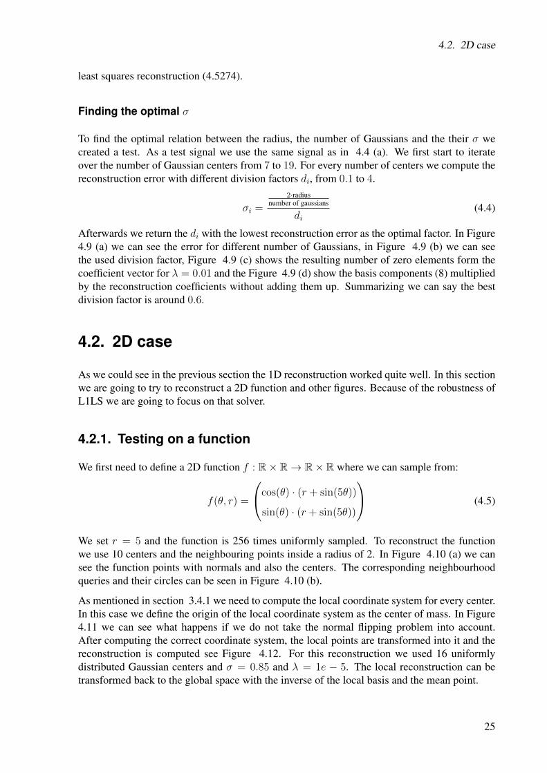
To find the optimal relation between the radius, the number of Gaussians and the their σ wecreated a test. As a test signal we use the same signal as in 4.4 (a). We first start to iterateover the number of Gaussian centers from 7 to 19. For every number of centers we compute thereconstruction error with different division factors di, from 0.1 to 4.

σi =

2·radiusnumber of gaussians

di(4.4)

Afterwards we return the di with the lowest reconstruction error as the optimal factor. In Figure4.9 (a) we can see the error for different number of Gaussians, in Figure 4.9 (b) we can seethe used division factor, Figure 4.9 (c) shows the resulting number of zero elements form thecoefficient vector for λ = 0.01 and the Figure 4.9 (d) show the basis components (8) multipliedby the reconstruction coefficients without adding them up. Summarizing we can say the bestdivision factor is around 0.6.

4.2. 2D case

As we could see in the previous section the 1D reconstruction worked quite well. In this sectionwe are going to try to reconstruct a 2D function and other figures. Because of the robustness ofL1LS we are going to focus on that solver.

4.2.1. Testing on a function

We first need to define a 2D function f : R× R→ R× R where we can sample from:

f(θ, r) =

cos(θ) · (r + sin(5θ))

sin(θ) · (r + sin(5θ))

(4.5)

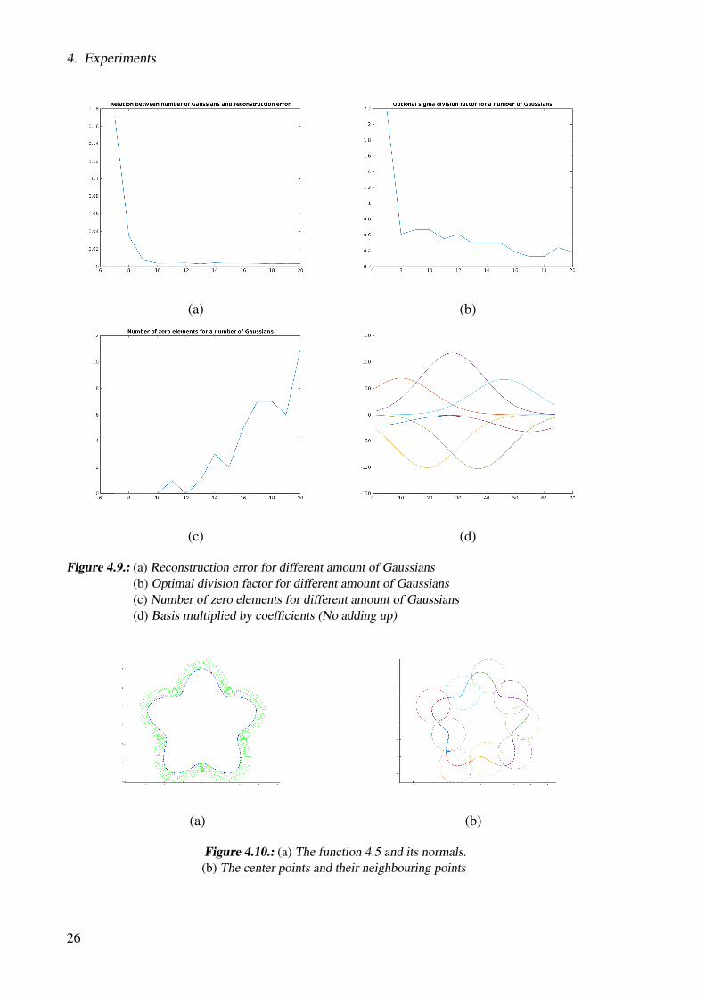
We set r = 5 and the function is 256 times uniformly sampled. To reconstruct the functionwe use 10 centers and the neighbouring points inside a radius of 2. In Figure 4.10 (a) we cansee the function points with normals and also the centers. The corresponding neighbourhoodqueries and their circles can be seen in Figure 4.10 (b).

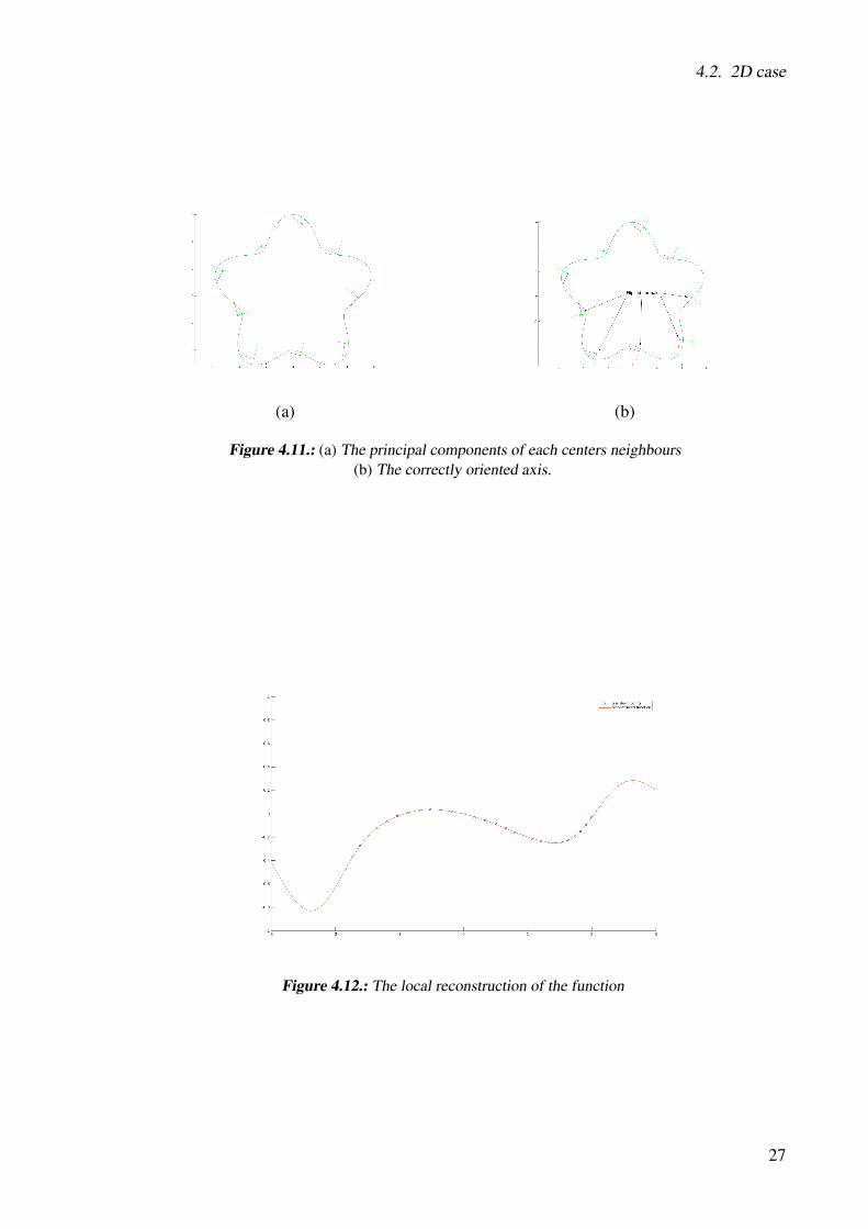
As mentioned in section 3.4.1 we need to compute the local coordinate system for every center.In this case we define the origin of the local coordinate system as the center of mass. In Figure4.11 we can see what happens if we do not take the normal flipping problem into account.After computing the correct coordinate system, the local points are transformed into it and thereconstruction is computed see Figure 4.12. For this reconstruction we used 16 uniformlydistributed Gaussian centers and σ = 0.85 and λ = 1e − 5. The local reconstruction can betransformed back to the global space with the inverse of the local basis and the mean point.

25

4. Experiments

(a) (b)

(c) (d)

Figure 4.9.: (a) Reconstruction error for different amount of Gaussians(b) Optimal division factor for different amount of Gaussians(c) Number of zero elements for different amount of Gaussians(d) Basis multiplied by coefficients (No adding up)

(a) (b)

Figure 4.10.: (a) The function 4.5 and its normals.(b) The center points and their neighbouring points

26

4.2. 2D case

(a) (b)

Figure 4.11.: (a) The principal components of each centers neighbours(b) The correctly oriented axis.

Figure 4.12.: The local reconstruction of the function

27

4. Experiments

(a) (b)

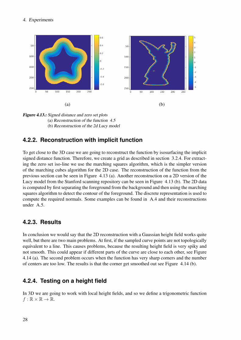
Figure 4.13.: Signed distance and zero set plots(a) Reconstruction of the function 4.5(b) Reconstruction of the 2d Lucy model

4.2.2. Reconstruction with implicit function

To get close to the 3D case we are going to reconstruct the function by isosurfacing the implicitsigned distance function. Therefore, we create a grid as described in section 3.2.4. For extract-ing the zero set iso-line we use the marching squares algorithm, which is the simpler versionof the marching cubes algorithm for the 2D case. The reconstruction of the function from theprevious section can be seen in Figure 4.13 (a). Another reconstruction on a 2D version of theLucy model from the Stanford scanning repository can be seen in Figure 4.13 (b). The 2D datais computed by first separating the foreground from the background and then using the marchingsquares algorithm to detect the contour of the foreground. The discrete representation is used tocompute the required normals. Some examples can be found in A.4 and their reconstructionsunder A.5.

4.2.3. Results

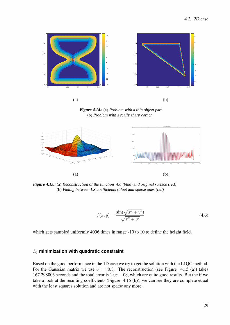
In conclusion we would say that the 2D reconstruction with a Gaussian height field works quitewell, but there are two main problems. At first, if the sampled curve points are not topologicallyequivalent to a line. This causes problems, because the resulting height field is very spiky andnot smooth. This could appear if different parts of the curve are close to each other, see Figure4.14 (a). The second problem occurs when the function has very sharp corners and the numberof centers are too low. The results is that the corner get smoothed out see Figure 4.14 (b).

4.2.4. Testing on a height field

In 3D we are going to work with local height fields, and so we define a trigonometric functionf : R× R→ R.

28

4.2. 2D case

(a) (b)

Figure 4.14.: (a) Problem with a thin object part(b) Problem with a really sharp corner.

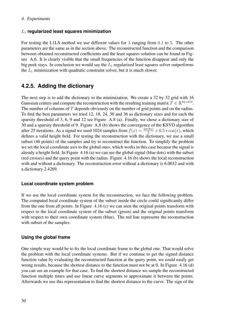
(a) (b)

Figure 4.15.: (a) Reconstruction of the function 4.6 (blue) and original surface (red)(b) Fading between LS coefficients (blue) and sparse ones (red)

f(x, y) =sin(

√x2 + y2)√x2 + y2

(4.6)

which gets sampled uniformly 4096 times in range -10 to 10 to define the height field.

L1 minimization with quadratic constraint

Based on the good performance in the 1D case we try to get the solution with the L1QC method.For the Gaussian matrix we use σ = 0.3. The reconstruction (see Figure 4.15 (a)) takes167.298803 seconds and the total error is 1.0e− 03, which are quite good results. But the if wetake a look at the resulting coefficients (Figure 4.15 (b)), we can see they are complete equalwith the least squares solution and are not sparse any more.

29

4. Experiments

L1 regularized least squares minimization

For testing the L1LS method we use different values for λ ranging from 0.1 to 5. The otherparameters are the same as in the section above. The reconstructed function and the comparisonbetween obtained reconstructed coefficients and the least squares solution can be found in Fig-ure A.6. It is clearly visible that the small frequencies of the function disappear and only thebig peek stays. In conclusion we would say the L1 regularized least squares solver outperformsthe L1 minimization with quadratic constraint solver, but it is much slower.

4.2.5. Adding the dictionary

The next step is to add the dictionary to the minimization. We create a 32 by 32 grid with 16Gaussian centers and compute the reconstruction with the resulting training matrix T ∈ R16×673.The number of columns of T depends obviously on the number of grid points and on the radius.To find the best parameters we tried 12, 18, 24, 30 and 36 as dictionary sizes and for each thesparsity threshold of 3, 6, 9 and 12 see Figure A.8 (a). Finally, we chose a dictionary size of30 and a sparsity threshold of 9. Figure A.8 (b) shows the convergence of the KSVD algorithmafter 25 iterations. As a signal we used 1024 samples from f(x) = sin(8x)

5+ 0.5 ∗ cos(x), which

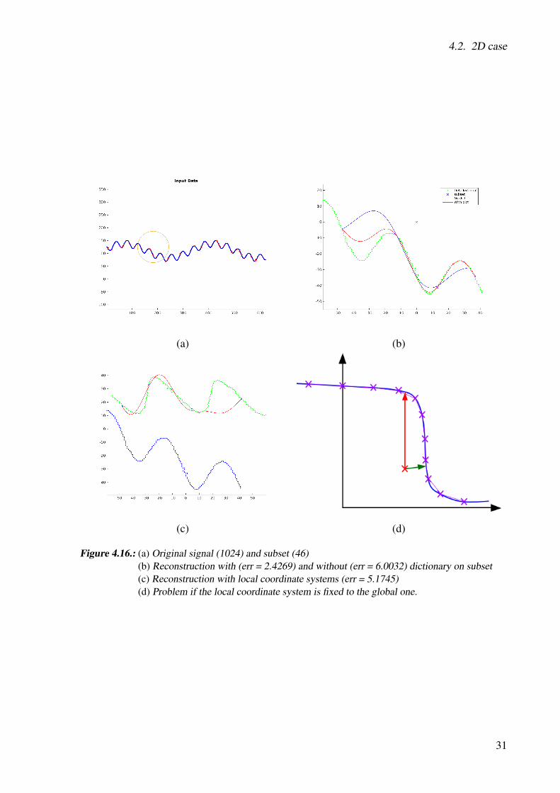
defines a valid height field. For testing the reconstruction with the dictionary, we use a smallsubset (46 points) of the samples and try to reconstruct the function. To simplify the problemwe set the local coordinate axis to the global ones, which works in this case because the signal isalready a height field. In Figure 4.16 (a) we can see the global signal (blue dots) with the subset(red crosses) and the query point with the radius. Figure 4.16 (b) shows the local reconstructionwith and without a dictionary. The reconstruction error without a dictionary is 6.0032 and witha dictionary 2.4269.

Local coordinate system problem

If we use the local coordinate system for the reconstruction, we face the following problem.The computed local coordinate system of the subset inside the circle could significantly differfrom the one from all points. In Figure 4.16 (c) we can seen the original points transform withrespect to the local coordinate system of the subset (green) and the original points transformwith respect to their own coordinate system (blue). The red line represents the reconstructionwith subset of the samples.

Using the global frame

One simple way would be to fix the local coordinate frame to the global one. That would solvethe problem with the local coordinate systems. But if we continue to get the signed distancefunction value by evaluating the reconstructed function at the query point, we could easily getwrong results, because the shortest distance to the function must not be at 0. In Figure 4.16 (d)you can see an example for that case. To find the shortest distance we sample the reconstructedfunction multiple times and use linear curve segments to approximate it between the points.Afterwards we use this representation to find the shortest distance to the curve. The sign of the

30

4.2. 2D case

(a) (b)

(c) (d)

Figure 4.16.: (a) Original signal (1024) and subset (46)(b) Reconstruction with (err = 2.4269) and without (err = 6.0032) dictionary on subset(c) Reconstruction with local coordinate systems (err = 5.1745)(d) Problem if the local coordinate system is fixed to the global one.

31

4. Experiments

(a) (b) (c)

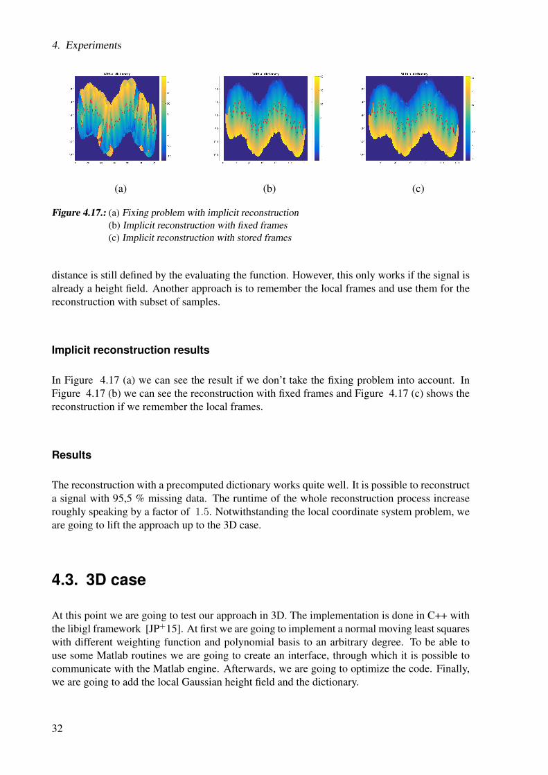
Figure 4.17.: (a) Fixing problem with implicit reconstruction(b) Implicit reconstruction with fixed frames(c) Implicit reconstruction with stored frames

distance is still defined by the evaluating the function. However, this only works if the signal isalready a height field. Another approach is to remember the local frames and use them for thereconstruction with subset of samples.

Implicit reconstruction results

In Figure 4.17 (a) we can see the result if we don’t take the fixing problem into account. InFigure 4.17 (b) we can see the reconstruction with fixed frames and Figure 4.17 (c) shows thereconstruction if we remember the local frames.

Results

The reconstruction with a precomputed dictionary works quite well. It is possible to reconstructa signal with 95,5 % missing data. The runtime of the whole reconstruction process increaseroughly speaking by a factor of 1.5. Notwithstanding the local coordinate system problem, weare going to lift the approach up to the 3D case.

4.3. 3D case

At this point we are going to test our approach in 3D. The implementation is done in C++ withthe libigl framework [JP+15]. At first we are going to implement a normal moving least squareswith different weighting function and polynomial basis to an arbitrary degree. To be able touse some Matlab routines we are going to create an interface, through which it is possible tocommunicate with the Matlab engine. Afterwards, we are going to optimize the code. Finally,we are going to add the local Gaussian height field and the dictionary.

32

4.3. 3D case

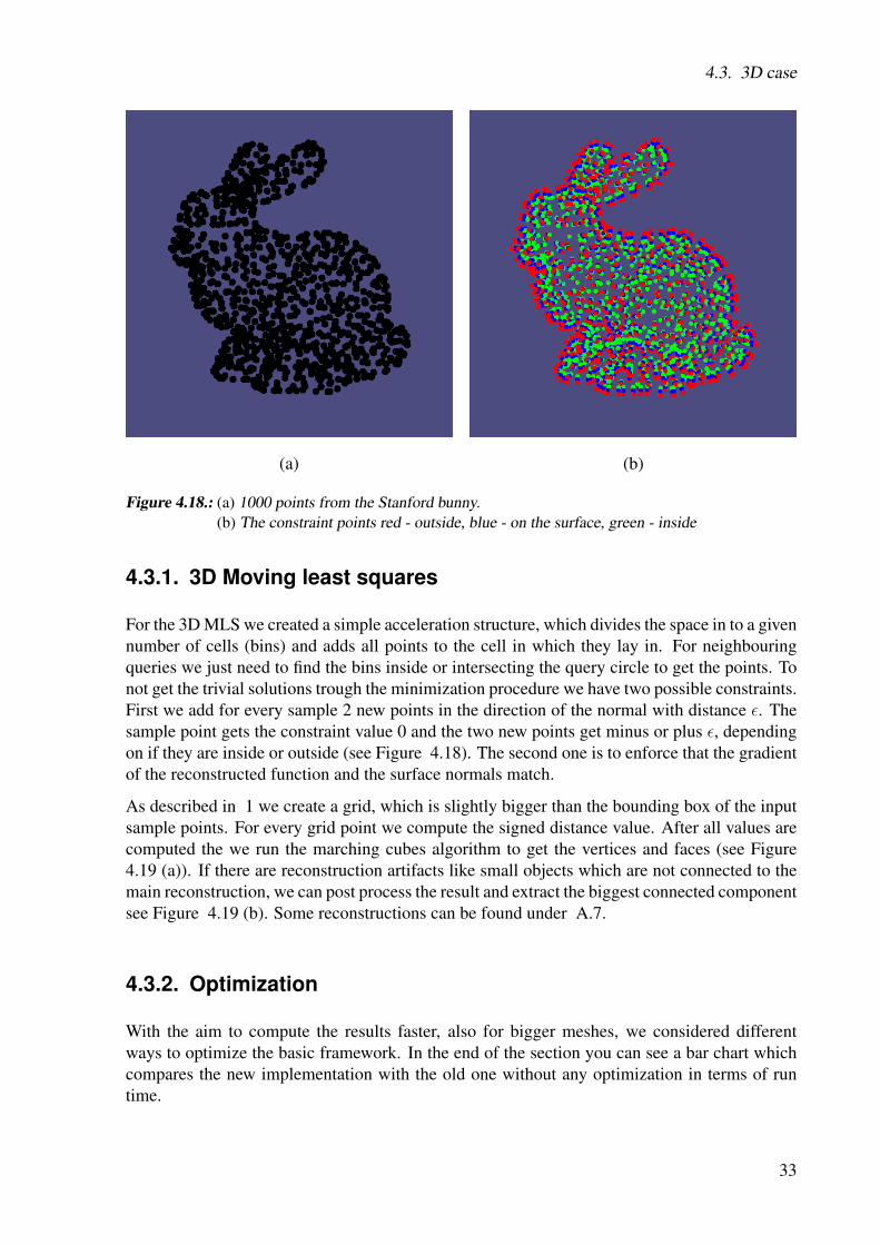
(a) (b)

Figure 4.18.: (a) 1000 points from the Stanford bunny.(b) The constraint points red - outside, blue - on the surface, green - inside

4.3.1. 3D Moving least squares

For the 3D MLS we created a simple acceleration structure, which divides the space in to a givennumber of cells (bins) and adds all points to the cell in which they lay in. For neighbouringqueries we just need to find the bins inside or intersecting the query circle to get the points. Tonot get the trivial solutions trough the minimization procedure we have two possible constraints.First we add for every sample 2 new points in the direction of the normal with distance ε. Thesample point gets the constraint value 0 and the two new points get minus or plus ε, dependingon if they are inside or outside (see Figure 4.18). The second one is to enforce that the gradientof the reconstructed function and the surface normals match.

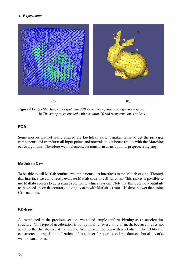
As described in 1 we create a grid, which is slightly bigger than the bounding box of the inputsample points. For every grid point we compute the signed distance value. After all values arecomputed the we run the marching cubes algorithm to get the vertices and faces (see Figure4.19 (a)). If there are reconstruction artifacts like small objects which are not connected to themain reconstruction, we can post process the result and extract the biggest connected componentsee Figure 4.19 (b). Some reconstructions can be found under A.7.

4.3.2. Optimization

With the aim to compute the results faster, also for bigger meshes, we considered differentways to optimize the basic framework. In the end of the section you can see a bar chart whichcompares the new implementation with the old one without any optimization in terms of runtime.

33

4. Experiments

(a) (b)

Figure 4.19.: (a) Marching cubes grid with SSD value blue - positive and green - negative.(b) The bunny reconstructed with resolution 20 and reconstructions artefacts.

PCA

Some meshes are not really aligned the Euclidean axis, it makes sense to get the principalcomponents and transform all input points and normals to get better results with the Marchingcubes algorithm. Therefore we implemented a transform as an optional preprocessing step.

Matlab in C++

To be able to call Matlab routines we implemented an interfaces to the Matlab engine. Throughthat interface we can directly evaluate Matlab code or call function. This makes it possible touse Matlabs solvers to get a sparse solution of a linear system. Note that this does not contributeto the speed up, on the contrary solving system with Matlab is around 10 times slower than usingC++ methods.

KD-tree

As mentioned in the previous section, we added simple uniform binning as an accelerationstructure. This type of acceleration is not optimal for every kind of mesh, because it does notadapt to the distribution of the points. We replaced the bin with a KD-tree. The KD-tree isconstructed during the initialization and is quicker for queries on large datasets, but also workswell on small ones.

34

4.3. 3D case

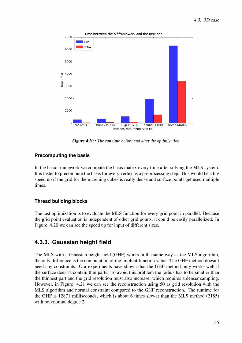
Figure 4.20.: The run time before and after the optimization.

Precomputing the basis

In the basic framework we compute the basis matrix every time after solving the MLS system.It is faster to precompute the basis for every vertex as a preprocessing step. This would be a bigspeed up if the grid for the marching cubes is really dense and surface points get used multipletimes.

Thread building blocks

The last optimization is to evaluate the MLS function for every grid point in parallel. Becausethe grid point evaluation is independent of other grid points, it could be easily parallelized. InFigure 4.20 we can see the speed up for input of different sizes.

4.3.3. Gaussian height field

The MLS with a Gaussian height field (GHF) works in the same way as the MLS algorithm,the only difference is the computation of the implicit function value. The GHF method doesn’tneed any constraints. Our experiments have shown that the GHF method only works well ifthe surface doesn’t contain thin parts. To avoid this problem the radius has to be smaller thanthe thinnest part and the grid resolution must also increase, which requires a denser sampling.However, in Figure 4.21 we can see the reconstruction using 50 as grid resolution with theMLS algorithm and normal constraint compared to the GHF reconstruction. The runtime forthe GHF is 12871 milliseconds, which is about 6 times slower than the MLS method (2185)with polynomial degree 2.

35

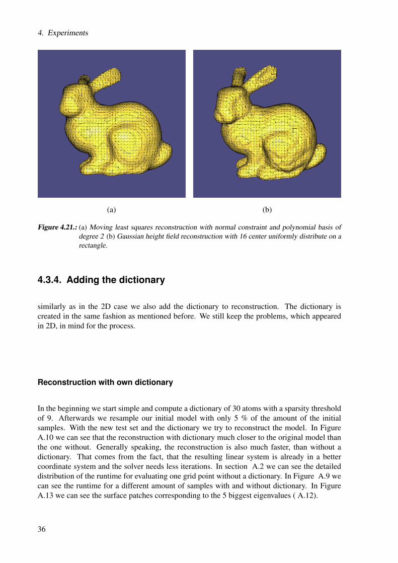
4. Experiments

(a) (b)

Figure 4.21.: (a) Moving least squares reconstruction with normal constraint and polynomial basis ofdegree 2 (b) Gaussian height field reconstruction with 16 center uniformly distribute on arectangle.

4.3.4. Adding the dictionary

similarly as in the 2D case we also add the dictionary to reconstruction. The dictionary iscreated in the same fashion as mentioned before. We still keep the problems, which appearedin 2D, in mind for the process.

Reconstruction with own dictionary

In the beginning we start simple and compute a dictionary of 30 atoms with a sparsity thresholdof 9. Afterwards we resample our initial model with only 5 % of the amount of the initialsamples. With the new test set and the dictionary we try to reconstruct the model. In FigureA.10 we can see that the reconstruction with dictionary much closer to the original model thanthe one without. Generally speaking, the reconstruction is also much faster, than without adictionary. That comes from the fact, that the resulting linear system is already in a bettercoordinate system and the solver needs less iterations. In section A.2 we can see the detaileddistribution of the runtime for evaluating one grid point without a dictionary. In Figure A.9 wecan see the runtime for a different amount of samples with and without dictionary. In FigureA.13 we can see the surface patches corresponding to the 5 biggest eigenvalues ( A.12).

36

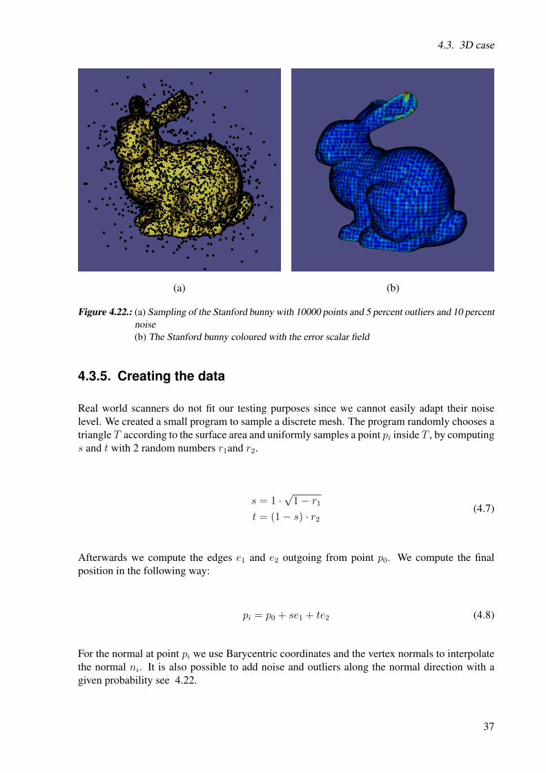
4.3. 3D case

(a) (b)

Figure 4.22.: (a) Sampling of the Stanford bunny with 10000 points and 5 percent outliers and 10 percentnoise(b) The Stanford bunny coloured with the error scalar field

4.3.5. Creating the data

Real world scanners do not fit our testing purposes since we cannot easily adapt their noiselevel. We created a small program to sample a discrete mesh. The program randomly chooses atriangle T according to the surface area and uniformly samples a point pi inside T , by computings and t with 2 random numbers r1and r2.

s = 1 ·√

1− r1t = (1− s) · r2

(4.7)

Afterwards we compute the edges e1 and e2 outgoing from point p0. We compute the finalposition in the following way:

pi = p0 + se1 + te2 (4.8)

For the normal at point pi we use Barycentric coordinates and the vertex normals to interpolatethe normal ni. It is also possible to add noise and outliers along the normal direction with agiven probability see 4.22.

37

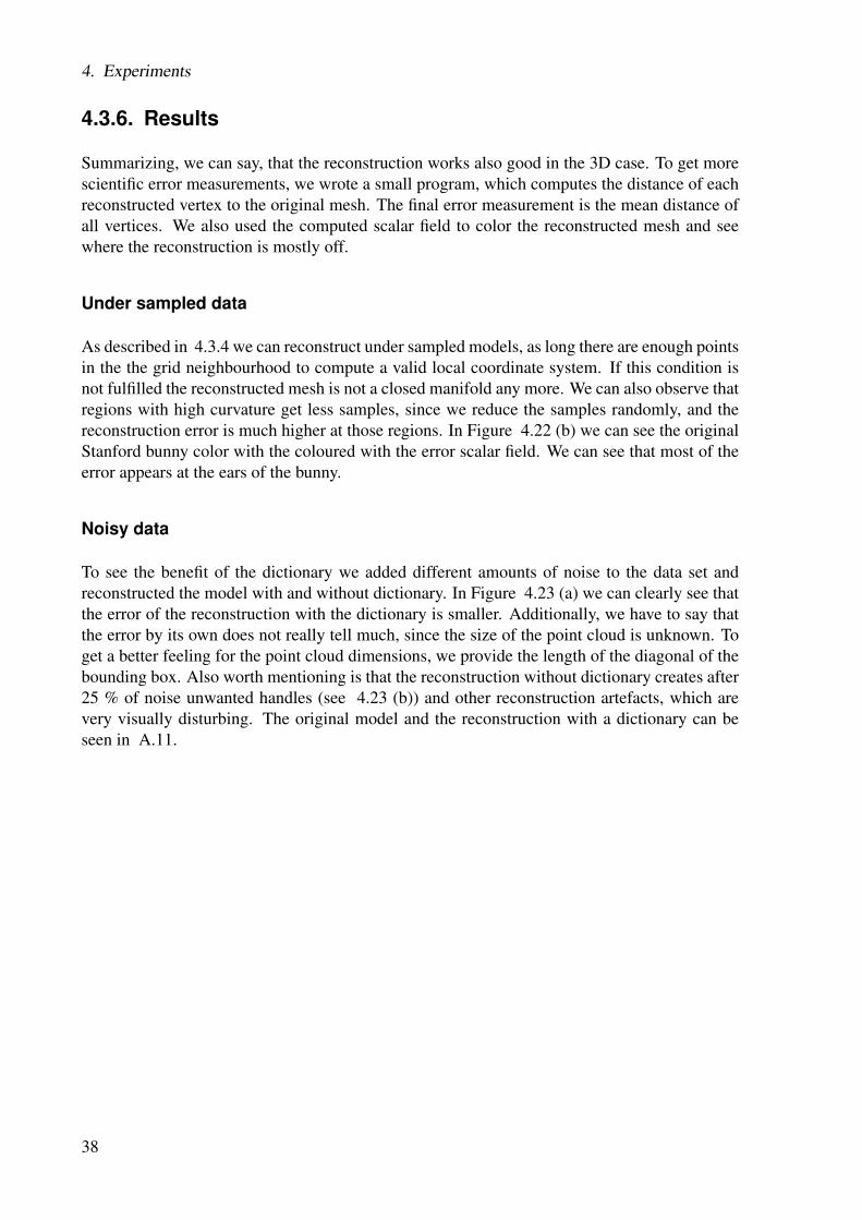
4. Experiments

4.3.6. Results

Summarizing, we can say, that the reconstruction works also good in the 3D case. To get morescientific error measurements, we wrote a small program, which computes the distance of eachreconstructed vertex to the original mesh. The final error measurement is the mean distance ofall vertices. We also used the computed scalar field to color the reconstructed mesh and seewhere the reconstruction is mostly off.

Under sampled data

As described in 4.3.4 we can reconstruct under sampled models, as long there are enough pointsin the the grid neighbourhood to compute a valid local coordinate system. If this condition isnot fulfilled the reconstructed mesh is not a closed manifold any more. We can also observe thatregions with high curvature get less samples, since we reduce the samples randomly, and thereconstruction error is much higher at those regions. In Figure 4.22 (b) we can see the originalStanford bunny color with the coloured with the error scalar field. We can see that most of theerror appears at the ears of the bunny.

Noisy data

To see the benefit of the dictionary we added different amounts of noise to the data set andreconstructed the model with and without dictionary. In Figure 4.23 (a) we can clearly see thatthe error of the reconstruction with the dictionary is smaller. Additionally, we have to say thatthe error by its own does not really tell much, since the size of the point cloud is unknown. Toget a better feeling for the point cloud dimensions, we provide the length of the diagonal of thebounding box. Also worth mentioning is that the reconstruction without dictionary creates after25 % of noise unwanted handles (see 4.23 (b)) and other reconstruction artefacts, which arevery visually disturbing. The original model and the reconstruction with a dictionary can beseen in A.11.

38

4.3. 3D case

(a) (b)

Figure 4.23.: (a) Reconstruction error plot (bounding boy diagonal 37.88875)(b) Reconstruction artefacts without dictionary

39

5Conclusion and Outlook

We introduced a new surface reconstruction technique which combines classical dictionarylearning and compressive sensing. First, the method computes a grid containing the signeddistance to the scanned data and extracts the zero level surface. Our approach makes recon-struction with undersampled or noisy point clouds possible.

In chapter 1 we started with a quick introduction and explained the importance of surface re-construction generally. In chapter 2 we gave a brief overview of the related work in the field ofsurface reconstruction, compressive sensing and dictionary learning. We discussed the advan-tages and disadvantages of the state-of-the-art methods and classified them into categories. Inthe next chapter we explained the theoretical background of our new reconstruction techniqueand step by step built the final minimization formulation. In our experiments we compareddifferent sparse solvers in terms of run time, reconstruction error and sparsity. We found outthat the L1 regularized least squares minimization mostly fitted our needs. We started to test thereconstruction from the one dimensional to the three dimensional case and documented prob-lems we encountered during this process and how we solved them. Furthermore, we did a lotof testing to find the best relationship between the available parameters and found those fewintuitive ones for the user. Finally, we can say that our method can keep up with the state-of-the-art methods with some requirements, like remembering and using the local coordinateframes. We contribute a modular reconstruction framework implemented in C++, which allowseasily to change or extent different parts, like the weighting function or the solver, from thereconstruction process.

Future work tackles the problem of the local frame approximation. To get more stable recon-structions, the local frames should not vary much if the number of points is decreased or noiseis added to the model. A possible way would be to take the normals into account and use themto compute the local coordinate system. Furthermore, the neighbourhood querying needs to beimproved, since in thin areas we get very spiky height fields resulting from the fact, that the

41

5. Conclusion and Outlook

local surface is not topologically equal to a disc. This problem could be solved by taking thenearest point as a start point and using very small sphere radii for the queries to incrementallyadd points to the local points, if they are still in the demanded search radius. This approachwould solve the problem, but also drastically increase the run time. Another suggestion to thisproblem would be to classify this situation as a problematic scenario and only use the samplesof the closer side. However, also in sharp regions like in corners or edges the method fails torepresent those and causes oversmoothing. To tackle this problem a different set of basis couldbe used, which can represent sharp features better than Gaussians. Finally, we want to create abetter dictionary, which is constructed with training data from a big amount of different pointclouds with different features and find out if we could get rid of some problems by optimizingthe used dictionary.

42

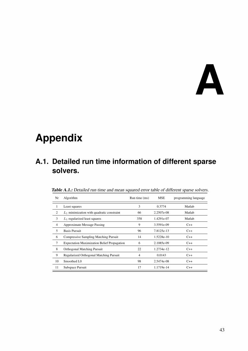
AAppendix

A.1. Detailed run time information of different sparsesolvers.

Table A.1.: Detailed run time and mean squared error table of different sparse solvers.

Nr Algorithm Run time (ms) MSE programming language

1 Least squares 3 0.3774 Matlab

2 L1 minimization with quadratic constraint 66 2.2507e-08 Matlab

3 L1 regularized least squares 358 1.4291e-07 Matlab

4 Approximate Message Passing 9 3.5591e-09 C++

5 Basis Pursuit 96 7.8125e-13 C++

6 Compressive Sampling Matching Pursuit 14 1.5228e-10 C++

7 Expectation Maximization Belief Propagation 6 2.1085e-09 C++

8 Orthogonal Matching Pursuit 22 1.2734e-12 C++

9 Regularized Orthogonal Matching Pursuit 4 0.0143 C++

10 Smoothed L0 98 2.5474e-08 C++

11 Subspace Pursuit 17 1.1719e-14 C++

43

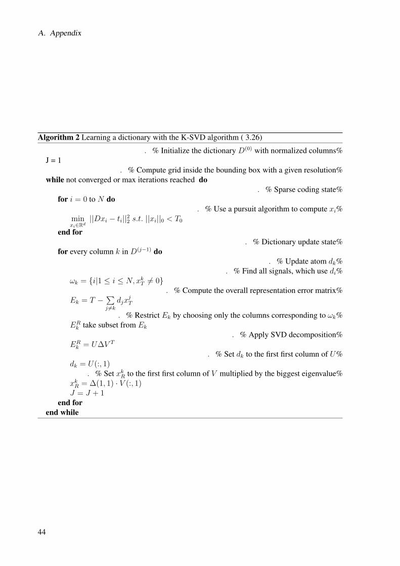
A. Appendix

Algorithm 2 Learning a dictionary with the K-SVD algorithm ( 3.26)

. % Initialize the dictionary D(0) with normalized columns%J = 1

. % Compute grid inside the bounding box with a given resolution%while not converged or max iterations reached do

. % Sparse coding state%for i = 0 to N do

. % Use a pursuit algorithm to compute xi%minxi∈Rd

||Dxi − ti||22 s.t. ||xi||0 < T0

end for. % Dictionary update state%

for every column k in D(j−1) do. % Update atom dk%

. % Find all signals, which use di%ωk = {i|1 ≤ i ≤ N, xkT 6= 0}

. % Compute the overall representation error matrix%Ek = T −

∑j 6=k

djxjT

. % Restrict Ek by choosing only the columns corresponding to ωk%ERk take subset from Ek

. % Apply SVD decomposition%ERk = U∆V T

. % Set dk to the first first column of U%dk = U(:, 1)

. % Set xkR to the first first column of V multiplied by the biggest eigenvalue%xkR = ∆(1, 1) · V (:, 1)J = J + 1

end forend while

44

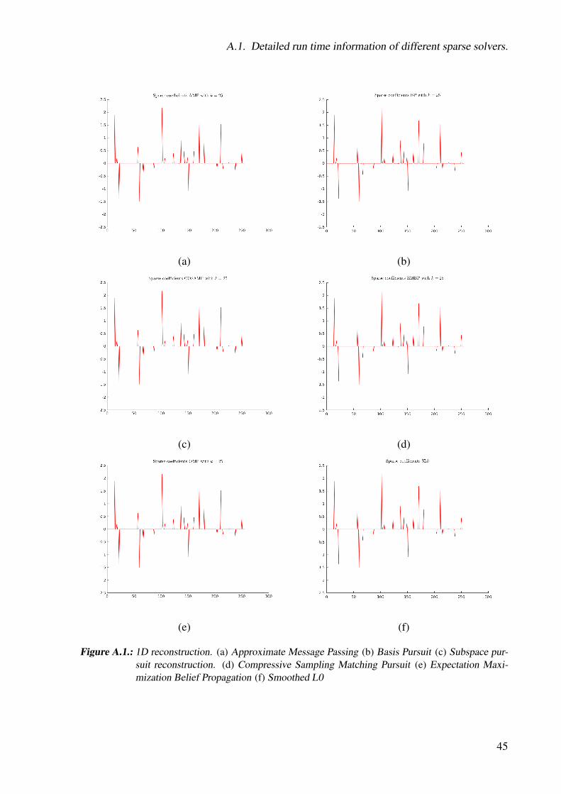
A.1. Detailed run time information of different sparse solvers.

(a) (b)

(c) (d)

(e) (f)

Figure A.1.: 1D reconstruction. (a) Approximate Message Passing (b) Basis Pursuit (c) Subspace pur-suit reconstruction. (d) Compressive Sampling Matching Pursuit (e) Expectation Maxi-mization Belief Propagation (f) Smoothed L0

45

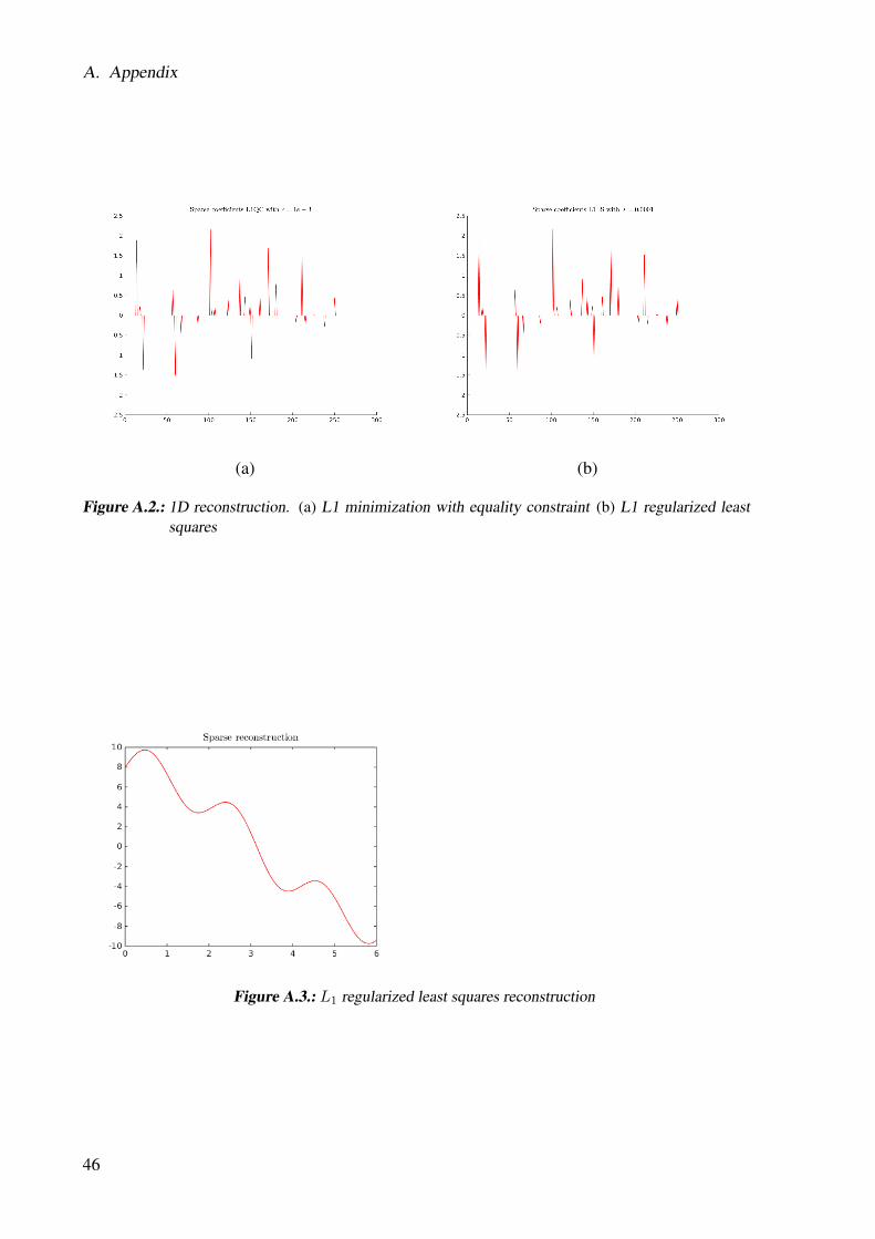
A. Appendix

(a) (b)

Figure A.2.: 1D reconstruction. (a) L1 minimization with equality constraint (b) L1 regularized leastsquares

Figure A.3.: L1 regularized least squares reconstruction

46

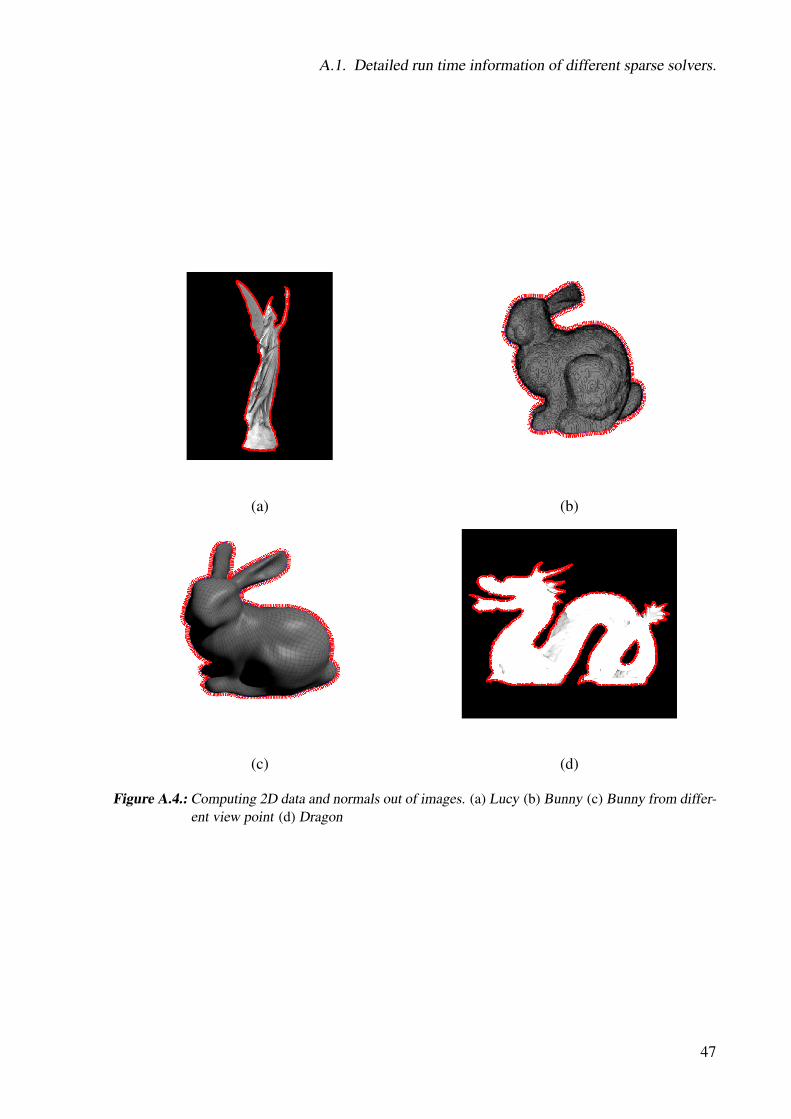
A.1. Detailed run time information of different sparse solvers.

(a) (b)

(c) (d)

Figure A.4.: Computing 2D data and normals out of images. (a) Lucy (b) Bunny (c) Bunny from differ-ent view point (d) Dragon

47

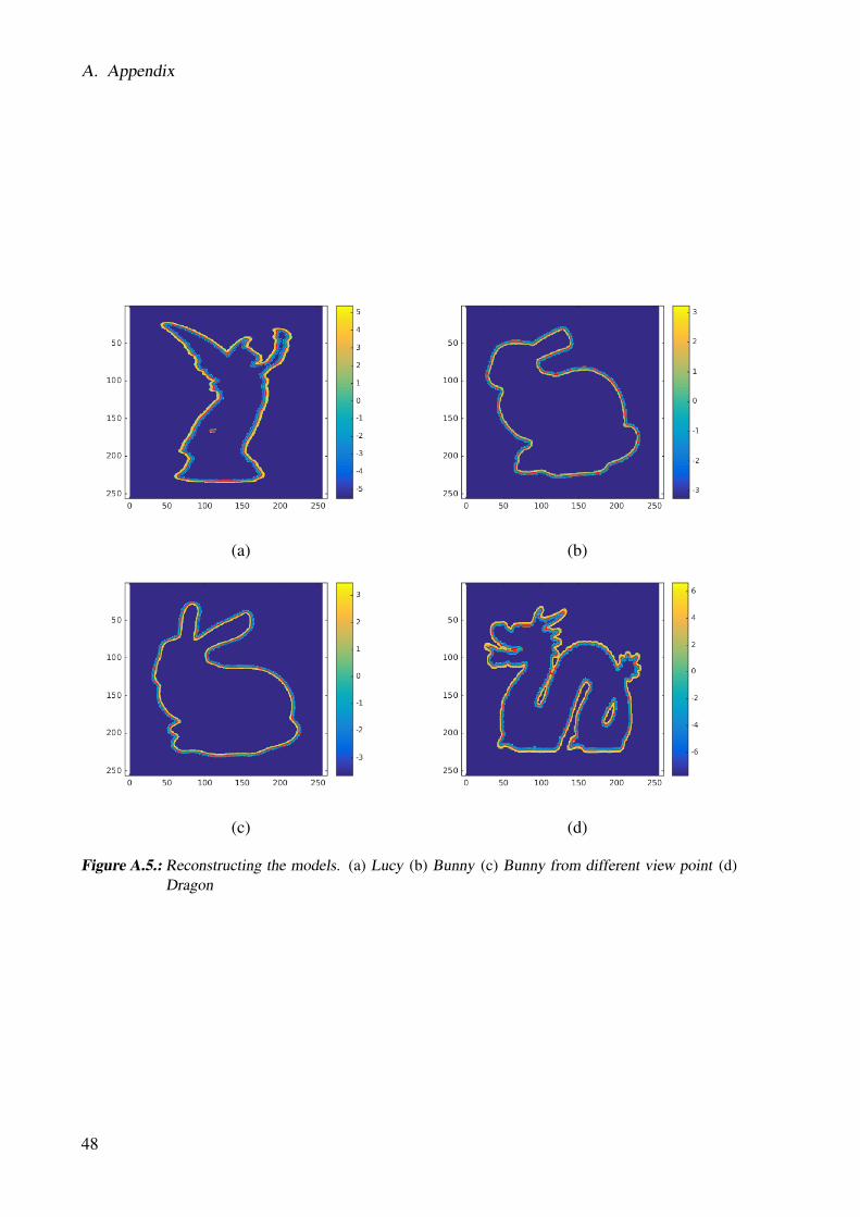
A. Appendix

(a) (b)

(c) (d)

Figure A.5.: Reconstructing the models. (a) Lucy (b) Bunny (c) Bunny from different view point (d)Dragon

48

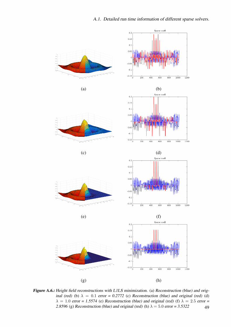
A.1. Detailed run time information of different sparse solvers.

(a) (b)

(c) (d)

(e) (f)

(g) (h)

Figure A.6.: Height field reconstructions with L1LS minimization. (a) Reconstruction (blue) and orig-inal (red) (b) λ = 0.1 error = 0.2772 (c) Reconstruction (blue) and original (red) (d)λ = 1.0 error = 1.5574 (e) Reconstruction (blue) and original (red) (f) λ = 2.5 error =2.8596 (g) Reconstruction (blue) and original (red) (h) λ = 5.0 error = 3.5322 49

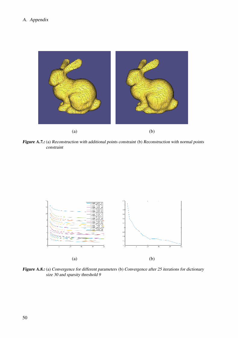
A. Appendix

(a) (b)

Figure A.7.: (a) Reconstruction with additional points constraint (b) Reconstruction with normal pointsconstraint

(a) (b)

Figure A.8.: (a) Convergence for different parameters (b) Convergence after 25 iterations for dictionarysize 30 and sparsity threshold 9

50

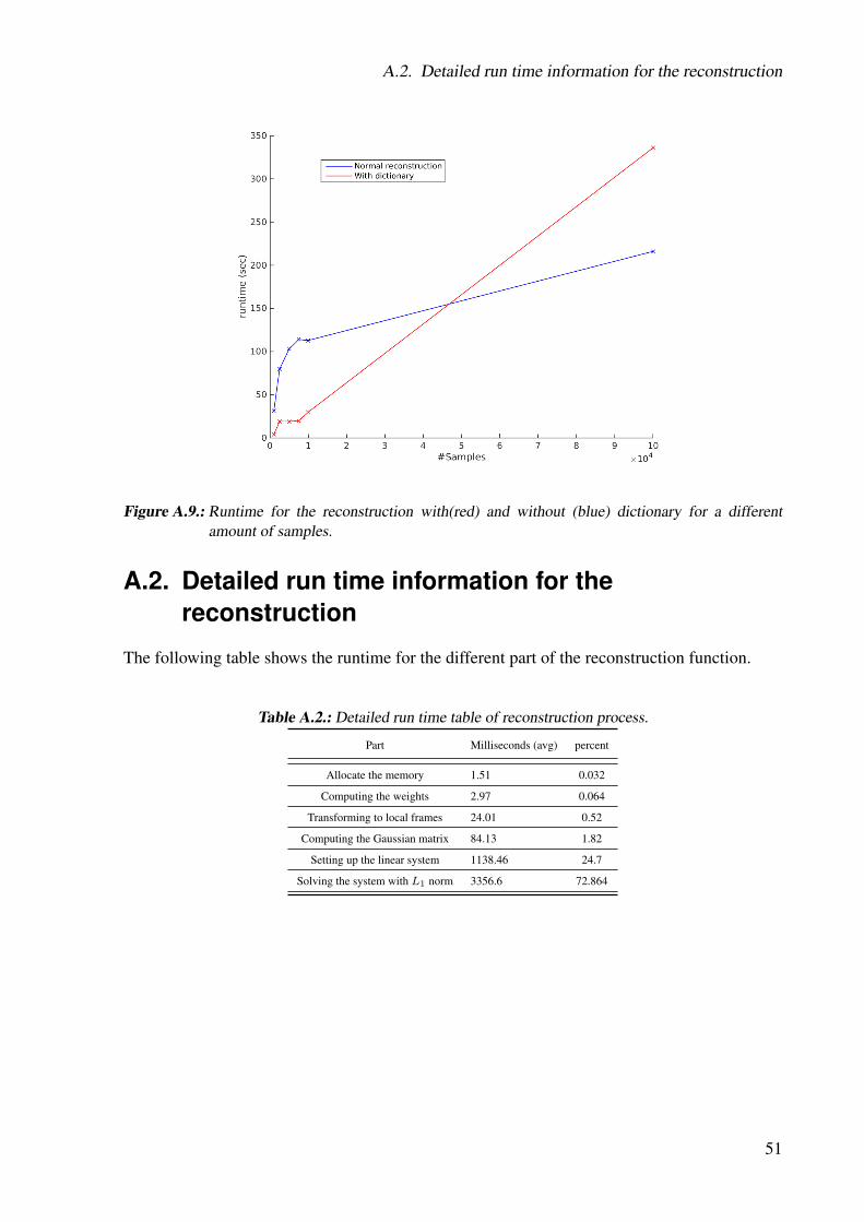
A.2. Detailed run time information for the reconstruction

Figure A.9.: Runtime for the reconstruction with(red) and without (blue) dictionary for a differentamount of samples.

A.2. Detailed run time information for thereconstruction

The following table shows the runtime for the different part of the reconstruction function.

Table A.2.: Detailed run time table of reconstruction process.

Part Milliseconds (avg) percent

Allocate the memory 1.51 0.032

Computing the weights 2.97 0.064

Transforming to local frames 24.01 0.52

Computing the Gaussian matrix 84.13 1.82

Setting up the linear system 1138.46 24.7

Solving the system with L1 norm 3356.6 72.864

51

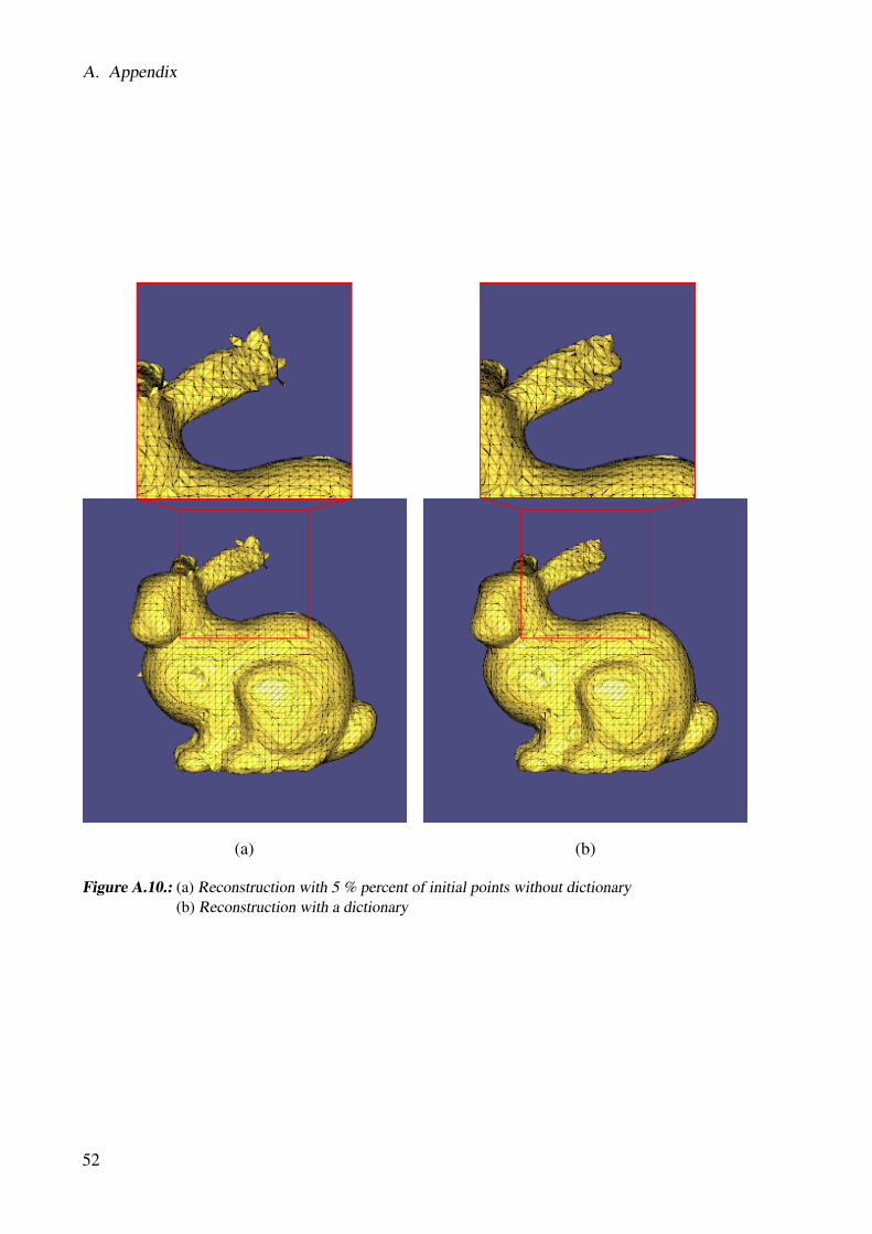
A. Appendix

(a) (b)

Figure A.10.: (a) Reconstruction with 5 % percent of initial points without dictionary(b) Reconstruction with a dictionary

52

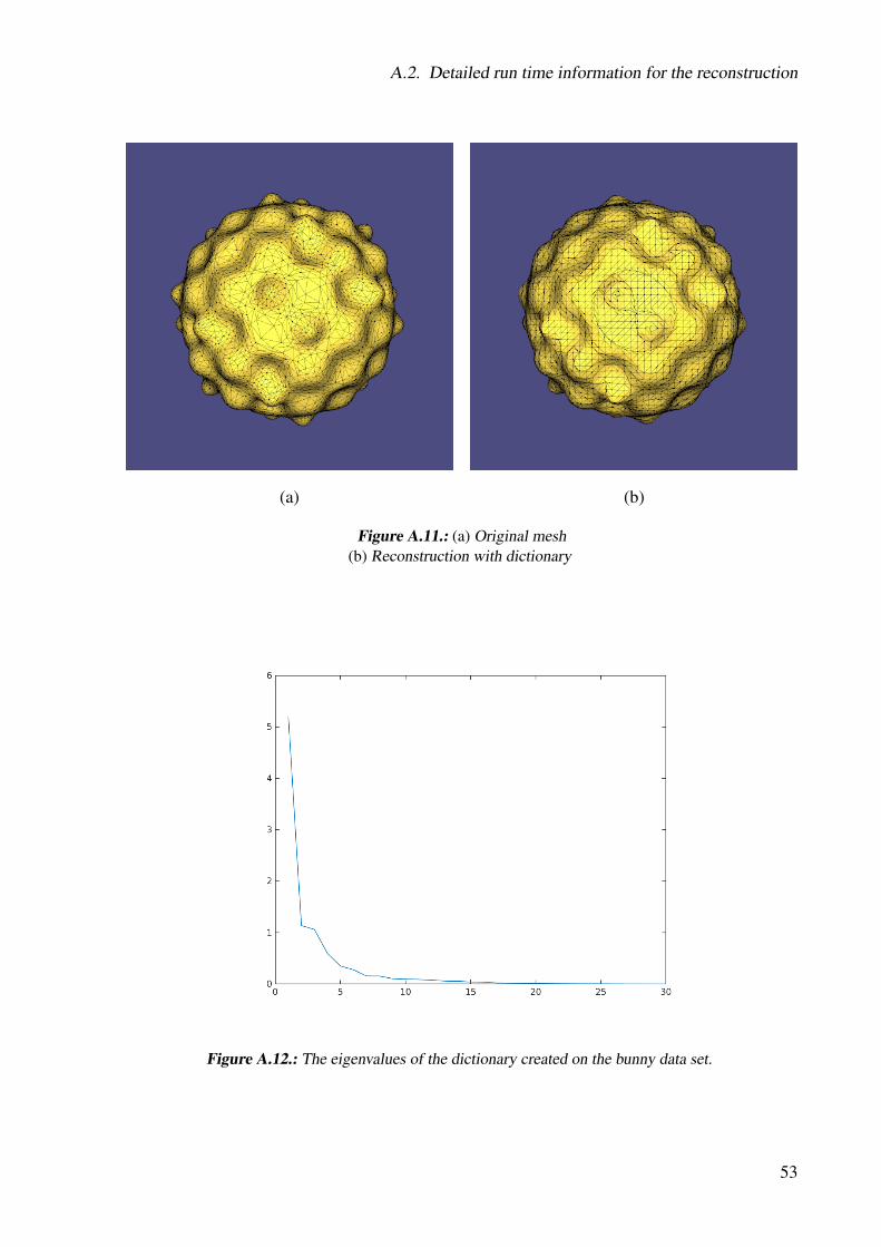
A.2. Detailed run time information for the reconstruction

(a) (b)

Figure A.11.: (a) Original mesh(b) Reconstruction with dictionary

Figure A.12.: The eigenvalues of the dictionary created on the bunny data set.

53

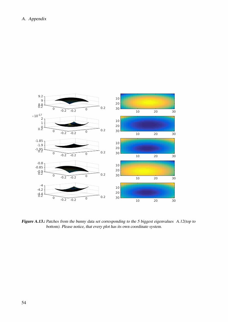
A. Appendix

Figure A.13.: Patches from the bunny data set corresponding to the 5 biggest eigenvalues A.12(top tobottom). Please notice, that every plot has its own coordinate system.

54

Bibliography

[ABCO+01] Marc Alexa, Johannes Behr, Daniel Cohen-Or, Shachar Fleishman, David Levin,and Claudio T. Silva. Point set surfaces. In Proceedings of the Conference onVisualization ’01, VIS ’01, pages 21–28, Washington, DC, USA, 2001. IEEEComputer Society.

[AEB06] M. Aharon, M. Elad, and A. Bruckstein. Svdd: An algorithm for designing over-complete dictionaries for sparse representation. Trans. Sig. Proc., 54(11):4311–4322, November 2006.

[ASGCO10] Haim Avron, Andrei Sharf, Chen Greif, and Daniel Cohen-Or. l1 sparse recon-struction of sharp point set surfaces. ACM Trans. Graph., 29(5):135:1–135:12,November 2010.

[BPC+11] Stephen Boyd, Neal Parikh, Eric Chu, Borja Peleato, and Jonathan Eckstein. Dis-tributed optimization and statistical learning via the alternating direction methodof multipliers. Found. Trends Mach. Learn., 3(1):1–122, January 2011.

[CBC+01] J. C. Carr, R. K. Beatson, J. B. Cherrie, T. J. Mitchell, W. R. Fright, B. C. Mc-Callum, and T. R. Evans. Reconstruction and representation of 3d objects withradial basis functions. In Proceedings of the 28th Annual Conference on Com-puter Graphics and Interactive Techniques, SIGGRAPH ’01, pages 67–76, NewYork, NY, USA, 2001. ACM.

[CG06] Frederic Cazals and Joachim Giesen. Delaunay triangulation based surface re-construction: Ideas and algorithms. In EFFECTIVE COMPUTATIONAL GEOM-ETRY FOR CURVES AND SURFACES, pages 231–273. Springer, 2006.

[Cle79] William S. Cleveland. Robust locally weighted regression and smoothing scatter-

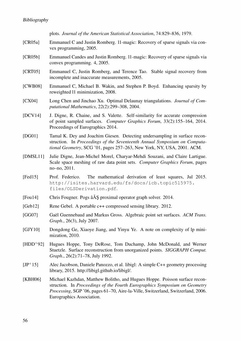
Bibliography

plots. Journal of the American Statistical Association, 74:829–836, 1979.

[CR05a] Emmanuel C and Justin Romberg. l1-magic: Recovery of sparse signals via con-vex programming, 2005.

[CR05b] Emmanuel Candes and Justin Romberg. l1-magic: Recovery of sparse signals viaconvex programming. 4, 2005.

[CRT05] Emmanuel C, Justin Romberg, and Terence Tao. Stable signal recovery fromincomplete and inaccurate measurements, 2005.

[CWB08] Emmanuel C, Michael B. Wakin, and Stephen P. Boyd. Enhancing sparsity byreweighted l1 minimization, 2008.

[CX04] Long Chen and Jinchao Xu. Optimal Delaunay triangulations. Journal of Com-putational Mathematics, 22(2):299–308, 2004.

[DCV14] J. Digne, R. Chaine, and S. Valette. Self-similarity for accurate compressionof point sampled surfaces. Computer Graphics Forum, 33(2):155–164, 2014.Proceedings of Eurographics 2014.

[DG01] Tamal K. Dey and Joachim Giesen. Detecting undersampling in surface recon-struction. In Proceedings of the Seventeenth Annual Symposium on Computa-tional Geometry, SCG ’01, pages 257–263, New York, NY, USA, 2001. ACM.

[DMSL11] Julie Digne, Jean-Michel Morel, Charyar-Mehdi Souzani, and Claire Lartigue.Scale space meshing of raw data point sets. Computer Graphics Forum, pagesno–no, 2011.

[Fed15] Prof. Federico. The mathematical derivation of least squares, Jul 2015.http://isites.harvard.edu/fs/docs/icb.topic515975.files/OLSDerivation.pdf.

[Fou14] Chris Fougner. Pogs âAS proximal operator graph solver. 2014.

[Geb12] Rene Gebel. A portable c++ compressed sensing library. 2012.

[GG07] Gaël Guennebaud and Markus Gross. Algebraic point set surfaces. ACM Trans.Graph., 26(3), July 2007.

[GJY10] Dongdong Ge, Xiaoye Jiang, and Yinyu Ye. A note on complexity of lp mini-mization, 2010.

[HDD+92] Hugues Hoppe, Tony DeRose, Tom Duchamp, John McDonald, and WernerStuetzle. Surface reconstruction from unorganized points. SIGGRAPH Comput.Graph., 26(2):71–78, July 1992.

[JP+15] Alec Jacobson, Daniele Panozzo, et al. libigl: A simple C++ geometry processinglibrary, 2015. http://libigl.github.io/libigl/.

[KBH06] Michael Kazhdan, Matthew Bolitho, and Hugues Hoppe. Poisson surface recon-struction. In Proceedings of the Fourth Eurographics Symposium on GeometryProcessing, SGP ’06, pages 61–70, Aire-la-Ville, Switzerland, Switzerland, 2006.Eurographics Association.

56

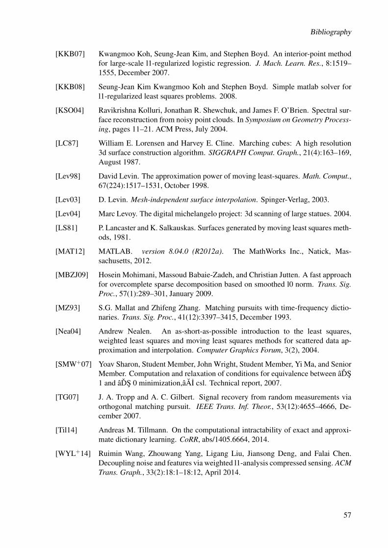
Bibliography

[KKB07] Kwangmoo Koh, Seung-Jean Kim, and Stephen Boyd. An interior-point methodfor large-scale l1-regularized logistic regression. J. Mach. Learn. Res., 8:1519–1555, December 2007.

[KKB08] Seung-Jean Kim Kwangmoo Koh and Stephen Boyd. Simple matlab solver forl1-regularized least squares problems. 2008.

[KSO04] Ravikrishna Kolluri, Jonathan R. Shewchuk, and James F. O’Brien. Spectral sur-face reconstruction from noisy point clouds. In Symposium on Geometry Process-ing, pages 11–21. ACM Press, July 2004.

[LC87] William E. Lorensen and Harvey E. Cline. Marching cubes: A high resolution3d surface construction algorithm. SIGGRAPH Comput. Graph., 21(4):163–169,August 1987.

[Lev98] David Levin. The approximation power of moving least-squares. Math. Comput.,67(224):1517–1531, October 1998.

[Lev03] D. Levin. Mesh-independent surface interpolation. Spinger-Verlag, 2003.

[Lev04] Marc Levoy. The digital michelangelo project: 3d scanning of large statues. 2004.

[LS81] P. Lancaster and K. Salkauskas. Surfaces generated by moving least squares meth-ods, 1981.

[MAT12] MATLAB. version 8.04.0 (R2012a). The MathWorks Inc., Natick, Mas-sachusetts, 2012.

[MBZJ09] Hosein Mohimani, Massoud Babaie-Zadeh, and Christian Jutten. A fast approachfor overcomplete sparse decomposition based on smoothed l0 norm. Trans. Sig.Proc., 57(1):289–301, January 2009.

[MZ93] S.G. Mallat and Zhifeng Zhang. Matching pursuits with time-frequency dictio-naries. Trans. Sig. Proc., 41(12):3397–3415, December 1993.

[Nea04] Andrew Nealen. An as-short-as-possible introduction to the least squares,weighted least squares and moving least squares methods for scattered data ap-proximation and interpolation. Computer Graphics Forum, 3(2), 2004.

[SMW+07] Yoav Sharon, Student Member, John Wright, Student Member, Yi Ma, and SeniorMember. Computation and relaxation of conditions for equivalence between âDS1 and âDS 0 minimization,âAI csl. Technical report, 2007.

[TG07] J. A. Tropp and A. C. Gilbert. Signal recovery from random measurements viaorthogonal matching pursuit. IEEE Trans. Inf. Theor., 53(12):4655–4666, De-cember 2007.

[Til14] Andreas M. Tillmann. On the computational intractability of exact and approxi-mate dictionary learning. CoRR, abs/1405.6664, 2014.

[WYL+14] Ruimin Wang, Zhouwang Yang, Ligang Liu, Jiansong Deng, and Falai Chen.Decoupling noise and features via weighted l1-analysis compressed sensing. ACMTrans. Graph., 33(2):18:1–18:12, April 2014.

57

Bibliography

[XZZ+14a] Shiyao Xiong, Juyong Zhang, Jianmin Zheng, Jianfei Cai, and Ligang Liu. Robustsurface reconstruction via dictionary learning. ACM Transactions on Graphics(Proc. SIGGRAPH Aisa), 33, 2014.

[XZZ+14b] Shiyao Xiong, Juyong Zhang, Jianmin Zheng, Jianfei Cai, and Ligang Liu. Robustsurface reconstruction via dictionary learning. ACM Trans. Graph., 33(6):201:1–201:12, November 2014.

58