Occlusion-Aware Multi-View Reconstruction of

Articulated Objects for Manipulation

A Dissertation

Presented to

the Graduate School of

Clemson University

In Partial Fulfillment

of the Requirements for the Degree

Doctor of Philosophy

Electrical Engineering

by

Xiaoxia Huang

August 2013

Accepted by:

Dr. Stanley T. Birchfield, Committee Chair

Dr. Ian D. Walker

Dr. John N. Gowdy

Dr. Damon L. Woodard

Abstract

The goal of this research is to develop algorithms using multiple views to

automatically recover complete 3D models of articulated objects in unstructured en-

vironments and thereby enable a robotic system to facilitate further manipulation of

those objects. First, an algorithm called Procrustes-Lo-RANSAC (PLR) is presented.

Structure-from-motion techniques are used to capture 3D point cloud models of an

articulated object in two different configurations. Procrustes analysis, combined with

a locally optimized RANSAC sampling strategy, facilitates a straightforward geomet-

ric approach to recovering the joint axes, as well as classifying them automatically as

either revolute or prismatic. The algorithm does not require prior knowledge of the

object, nor does it make any assumptions about the planarity of the object or scene.

Second, with such a resulting articulated model, a robotic system is then able

to manipulate the object either along its joint axes at a specified grasp point in order

to exercise its degrees of freedom or move its end effector to a particular position even

if the point is not visible in the current view. This is one of the main advantages of the

occlusion-aware approach, because the models capture all sides of the object meaning

that the robot has knowledge of parts of the object that are not visible in the current

view. Experiments with a PUMA 500 robotic arm demonstrate the effectiveness of

the approach on a variety of real-world objects containing both revolute and prismatic

joints.

ii

Third, we improve the proposed approach by using a RGBD sensor (Microsoft

Kinect) that yield a depth value for each pixel immediately by the sensor itself rather

than requiring correspondence to establish depth. KinectFusion algorithm is applied

to produce a single high-quality, geometrically accurate 3D model from which rigid

links of the object are segmented and aligned, allowing the joint axes to be estimated

using the geometric approach. The improved algorithm does not require artificial

markers attached to objects, yields much denser 3D models and reduces the compu-

tation time.

iii

Dedication

I dedicate this work to my beloved family who made all of this possible for

their endless encouragement and faith.

iv

Acknowledgments

First, I would like to give my most heartfelt thanks to my adviser, Dr. Stanley

Birchfield for his numerous guidance and support at every step of this work. His deep

love and insight of science inspired me in the right direction and made my journey

a truly enjoyable learning experience which will guild me throughout my life. He is

always patient, encouraging and enlightening. Additionally, I am very grateful to Dr.

Ian D. Walker, Dr. John N. Gowdy, and Dr. Damon L. Woodard, for their valuable

input and instruction in directing the research to this point.

My gratitude is also extended to all the members of my research group who

directly and indirectly provided helpful discussion, and assistance. Also I would like

to thank all my friends at Clemson supporting me all the time.

Finally, I would like to thank my family for their immense love, support, and

patience.

v

Table of Contents

Title Page . . . . . . . . . . . . . . . . . . . . . . . . . . . . . . . . . . . i

Abstract . . . . . . . . . . . . . . . . . . . . . . . . . . . . . . . . . . . . ii

Dedication . . . . . . . . . . . . . . . . . . . . . . . . . . . . . . . . . . . iv

Acknowledgments . . . . . . . . . . . . . . . . . . . . . . . . . . . . . . . v

List of Tables . . . . . . . . . . . . . . . . . . . . . . . . . . . . . . . . . viii

List of Figures . . . . . . . . . . . . . . . . . . . . . . . . . . . . . . . . . ix

1 Introduction . . . . . . . . . . . . . . . . . . . . . . . . . . . . . . . . 11.1 Robot manipulation . . . . . . . . . . . . . . . . . . . . . . . . . . . 11.2 Articulated objects . . . . . . . . . . . . . . . . . . . . . . . . . . . . 51.3 Outline of dissertation . . . . . . . . . . . . . . . . . . . . . . . . . . 8

2 Related Work . . . . . . . . . . . . . . . . . . . . . . . . . . . . . . . 102.1 Multi-view reconstruction . . . . . . . . . . . . . . . . . . . . . . . . 102.2 Articulated structure . . . . . . . . . . . . . . . . . . . . . . . . . . . 152.3 Object manipulation . . . . . . . . . . . . . . . . . . . . . . . . . . . 17

3 Learning Articulated Objects . . . . . . . . . . . . . . . . . . . . . . 183.1 Building initial 3D model . . . . . . . . . . . . . . . . . . . . . . . . . 203.2 Rigid link segmentation . . . . . . . . . . . . . . . . . . . . . . . . . 223.3 Classifying joints . . . . . . . . . . . . . . . . . . . . . . . . . . . . . 263.4 Finding joint axes . . . . . . . . . . . . . . . . . . . . . . . . . . . . . 273.5 Experimental results . . . . . . . . . . . . . . . . . . . . . . . . . . . 36

4 Manipulating Articulated Objects . . . . . . . . . . . . . . . . . . . 434.1 Hand-eye calibration . . . . . . . . . . . . . . . . . . . . . . . . . . . 454.2 Object pose estimation . . . . . . . . . . . . . . . . . . . . . . . . . . 484.3 Experimental results . . . . . . . . . . . . . . . . . . . . . . . . . . . 53

5 Using RGBD Sensors . . . . . . . . . . . . . . . . . . . . . . . . . . . 61

vi

5.1 RGBD sensors . . . . . . . . . . . . . . . . . . . . . . . . . . . . . . . 615.2 KinectFusion . . . . . . . . . . . . . . . . . . . . . . . . . . . . . . . 705.3 Learning articulated objects . . . . . . . . . . . . . . . . . . . . . . . 76

6 Conclusion . . . . . . . . . . . . . . . . . . . . . . . . . . . . . . . . . 836.1 Contributions . . . . . . . . . . . . . . . . . . . . . . . . . . . . . . . 846.2 Future work . . . . . . . . . . . . . . . . . . . . . . . . . . . . . . . . 85

Bibliography . . . . . . . . . . . . . . . . . . . . . . . . . . . . . . . . . . 87

vii

List of Tables

3.1 The quantitative assessment of the algorithms. . . . . . . . . . . . . . 41

4.1 The camera intrinsic parameters. . . . . . . . . . . . . . . . . . . . . 554.2 The relative robot hand poses. . . . . . . . . . . . . . . . . . . . . . . 58

viii

List of Figures

1.1 Examples of robots. . . . . . . . . . . . . . . . . . . . . . . . . . . . . 21.2 Two-link articulated object models . . . . . . . . . . . . . . . . . . . 61.3 Examples of articulated objects. . . . . . . . . . . . . . . . . . . . . . 6

2.1 A 2D example of the visual hull. . . . . . . . . . . . . . . . . . . . . . 13

3.1 Overview of the system. . . . . . . . . . . . . . . . . . . . . . . . . . 193.2 The PUMA 500 robotic arm manipulation. . . . . . . . . . . . . . . . 193.3 3D models with camera locations of a toy truck. . . . . . . . . . . . . 213.4 The dense 3D reconstruction of a toy truck. . . . . . . . . . . . . . . 223.5 Aligning an object with two links and two configurations in 2D. . . . 283.6 An illustration of the axis of rotation in 2D. . . . . . . . . . . . . . . 313.7 An illustration of the translation in 2D. . . . . . . . . . . . . . . . . . 323.8 The axis of rotation u. . . . . . . . . . . . . . . . . . . . . . . . . . . 353.9 Axis estimation of the truck. . . . . . . . . . . . . . . . . . . . . . . . 373.10 Axis estimation of a synthetic refrigerator. . . . . . . . . . . . . . . . 383.11 Five examples of articulated reconstruction. . . . . . . . . . . . . . . 393.12 Results of related work. . . . . . . . . . . . . . . . . . . . . . . . . . . 403.13 Articulated reconstruction of multiple-axis objects. . . . . . . . . . . 42

4.1 Three calibrations of a robotic system. . . . . . . . . . . . . . . . . . 444.2 Hand-eye calibration setup. . . . . . . . . . . . . . . . . . . . . . . . 464.3 Camera calibration setup. . . . . . . . . . . . . . . . . . . . . . . . . 494.4 Scaled orthographic projection and perspective projection. . . . . . . 524.5 Chessboard images for hand-eye calibration. . . . . . . . . . . . . . . 544.6 Extracted corners on chessboard images for hand-eye calibration. . . 554.7 The camera extrinsic parameters. . . . . . . . . . . . . . . . . . . . . 564.8 Extracted corners and their reprojected points. . . . . . . . . . . . . . 564.9 Two example images captured for manipulation. . . . . . . . . . . . . 594.10 Comparison of SIFT and ASIFT feature matching. . . . . . . . . . . 604.11 A video sequence of the robot manipulation. . . . . . . . . . . . . . . 60

5.1 Pinhole camera model. . . . . . . . . . . . . . . . . . . . . . . . . . . 635.2 Standard stereo model for two pinhole cameras. . . . . . . . . . . . . 645.3 General stereo model for two non-parallel cameras. . . . . . . . . . . 65

ix

5.4 Simple structured light 3D scanner model. . . . . . . . . . . . . . . . 665.5 A pulsed time-of-flight system. . . . . . . . . . . . . . . . . . . . . . . 675.6 Microsoft Kinect diagram. . . . . . . . . . . . . . . . . . . . . . . . . 685.7 Light pattern used by Microsoft Kinect. . . . . . . . . . . . . . . . . 695.8 Overview of KinectFusion algorithm. . . . . . . . . . . . . . . . . . . 705.9 IR image. . . . . . . . . . . . . . . . . . . . . . . . . . . . . . . . . . 715.10 Depth image of a microwave in an office environment. . . . . . . . . . 725.11 Camera tracking in KinectFusion. . . . . . . . . . . . . . . . . . . . . 745.12 A TSDF volume grid. . . . . . . . . . . . . . . . . . . . . . . . . . . . 755.13 Ray-casting. . . . . . . . . . . . . . . . . . . . . . . . . . . . . . . . . 765.14 Overview of the system using Kinect sensor. . . . . . . . . . . . . . . 775.15 Images and 3D models of a microwave. . . . . . . . . . . . . . . . . . 785.16 Images and 3D models of a microwave in a different configuration. . . 795.17 Images of opening the door of a microwave. . . . . . . . . . . . . . . . 805.18 Estimated rotation axis of a microwave. . . . . . . . . . . . . . . . . . 82

x

Chapter 1

Introduction

1.1 Robot manipulation

Since Unimate, the first industrial robot, designed by George Devol for a pro-

duction line at the General Motors Ternstedt plant in Trenton, NJ, in 1961, robots

have been widely used in a variety of areas such as manufacturing, medical, services,

environment, transportation, entertainment and education in the past half century

[3, 29, 68]. Figure 1.1 shows several examples of robots. As the primary application,

industrial robots are used to perform operations such as welding, assembly, painting,

picking and placing quickly, repeatedly and accurately in tedious and dangerous man-

ufacturing environments to improve safety and efficiency of production and reduce

environmental impact. Over the last three decades robotics has been integrated by

medical industries to aid surgeons, and augment healthcare rehabilitation or training

using more precise and less invasive methods. In the domestic applications, people

have had increasing needs for robots to assist their daily lives for example cleaning

houses, mowing lawns or delivering stuff in order to improve the quality of life. Since

robotics involves multiple disciplines like mathematics, physics, computer science and

1

Figure 1.1: Examples of robots: Surgical System Robot (DaVinci), UMass MobileManipulator (UMass Amherst), Mirra Pool-cleaning Robot (iRobot), Nao HumanoidRobot (Aldebaran).

so forth, robotic toys and educational toolkits are widely introduced to help students

to deeply understand basic concepts of such disciplines and inspire students to design,

innovate and solve problems.

Up to now, the development of robots is roughly divided into three stages

[68, 69]. The first generation is to perform simple and predictable tasks in constrained

industrial environments, for example robotic arms, which have similar functions of

human arms, assembling cars, handling machine tools or packaging food boxes. How-

ever, for real world applications functionality and environments often change. People

need robots to have capabilities to serve autonomously. In order to satisfy these

needs, the second generation incorporates a sensor system and a computer into a

more complicated control system which analyzes various environmental information

collected by the sensor system and plans corresponding operations for execution by

the computer system [68]. The behaviors of such robots are largely limited by their

control systems which memorize the knowledge about their structured surroundings.

As robots move into unstructured environments such as homes, schools, and work-

places, it is unrealistic to expect robots to have advanced knowledge of all objects

that will be encountered in the physical world, and they may not be able to function

autonomously. Therefore the current generation introduces artificial intelligence into

2

the control system to enable robots to fully serve autonomously, or at least semi-

autonomously in unstructured, dynamic environments. This transition is perhaps

most apparent in the nascent emergence of socially assistive and service robotics ap-

plications in which robots help people in their homes and workplaces with basic tasks

such as cleaning, personalized care, and behavioral therapy. Such application areas

are expected to represent a key area of growth for the robotics industry for the coming

years.

To handle unstructured, unpredictable environments robots face many chal-

lenges in several aspects. At first, robots must improve their mobility to perform

tasks. Currently most robots navigate in an environment either by using a priori

map of the complete surrounding or building the environmental map as they move

through it [7]. Such map-based navigation systems only work in specific places. How-

ever, real world environments have much variability and uncertainty [3, 47]. To deal

with these difficulties, robotic systems need to introduce new representations of the

environment such as 3D maps, use novel sensing models like RGBD sensors or improve

current localization algorithms.

Second, dynamic and uncontrolled environments make robots manipulation

such as opening doors, doing laundries or cleaning kitchens more challenging [59, 60,

39]. To successfully interact with its surrounding, robotic systems typically make

assumptions of known features or models of objects in a scene. Even in a structured

environment, manipulation tasks are not easy with such assumptions. For example in

a cleaning-kitchen robotic system, it is not realistic to have knowledge of all types of

dishes and cups. Therefore real world environments impose many difficulties on robot

manipulations due to their uncertainty and complexity. In order to perform tasks and

manipulations in open and unstructured environments in which prior knowledges and

models are not available, robots need to develop abilities to actively learn about the

3

environments.

Third, robotic systems need to increase their sensing abilities to function au-

tonomously in unstructured environments. The goal of a robot sensor system is

to collect all information of its surrounding by “seeing,” “touching,” “feeling” and

“hearing.” Visual sensing serves as the “eyes” of robots which typically analyze and

process images captured by cameras or other visual sensors to understand environ-

ments. Visual sensing is one of the most promising ways to explore and learn about

the environment. Generally, computer vision techniques are used to analyze the sen-

sory streams in a passive manner, and recently significant progress has been achieved

with feature detectors and 3D reconstruction techniques. It is only natural to inves-

tigate how to apply techniques from computer vision to robotics applications rather

than concentrate on only visual sensing or machine manipulation separately. The

notion of active vision is that for some tasks the sensing problem can actually be

made more tractable by actively affecting visual streams by controlling the sensors.

However, in some cases the sensing system fails because of noisy sensor data

and ambiguities of real world. For example, due to noise it is hard to detect corre-

spondences between images which is a very common problem in robotic applications,

or robots may not recognize different objects such as plums and apples because they

have similar appearances in some viewpoints of cameras [3, 47]. Such problems are

difficult even in a fixed environment. They can be partially solved by adding more

constraints about objects’ position, color, dimension and other features. To handle

unstructured, unpredictable environments, new sensing devices and approaches will

be needed. In particular, rather than assuming that the robot has advanced knowl-

edge of all the objects that will be encountered, the robot must be able to actively

learn about its environment in order to effectively manipulate within it.

4

1.2 Articulated objects

Within the context of learning about the environment, one problem that has

caught the attention of robotics researchers recently is that of reconstructing articu-

lated objects [48, 89, 90, 91]. An articulated object can be modeled as a set of rigid

links connected by one or more joints, either revolute or prismatic. Much of the in-

formation about articulated objects is encoded in the relative motion of objects such

as human limbs moving with respect to the body, vehicle wheels moving in different

ways from the main body of the vehicle, and so forth. Many applications such as

household, elder care robots require the manipulation of such objects. While current

manipulation systems often assume a priori object models, articulated objects pose

an additional problem in that their structure changes dynamically. In order to per-

form manipulation tasks with such objects, it will be necessary to develop models

that capture their articulation behavior.

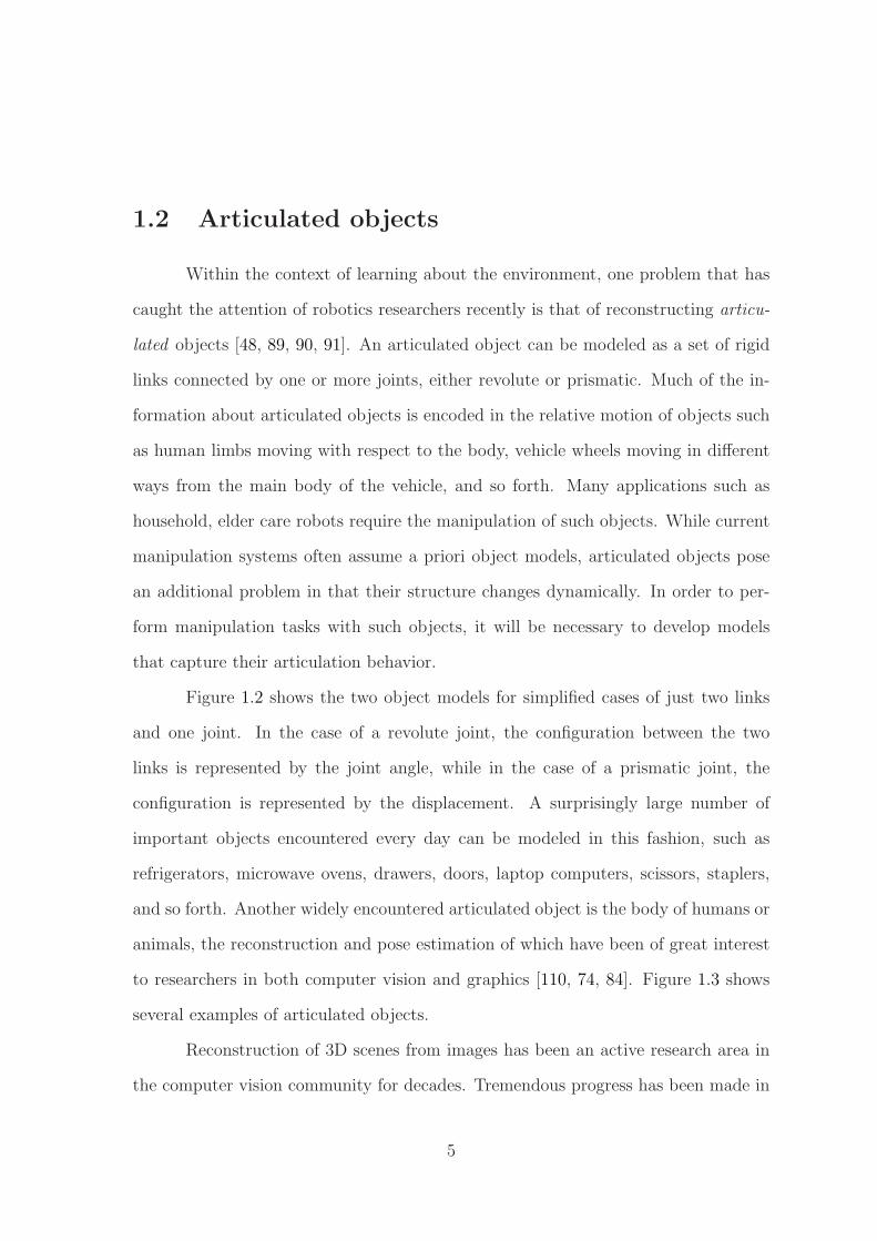
Figure 1.2 shows the two object models for simplified cases of just two links

and one joint. In the case of a revolute joint, the configuration between the two

links is represented by the joint angle, while in the case of a prismatic joint, the

configuration is represented by the displacement. A surprisingly large number of

important objects encountered every day can be modeled in this fashion, such as

refrigerators, microwave ovens, drawers, doors, laptop computers, scissors, staplers,

and so forth. Another widely encountered articulated object is the body of humans or

animals, the reconstruction and pose estimation of which have been of great interest

to researchers in both computer vision and graphics [110, 74, 84]. Figure 1.3 shows

several examples of articulated objects.

Reconstruction of 3D scenes from images has been an active research area in

the computer vision community for decades. Tremendous progress has been made in

5

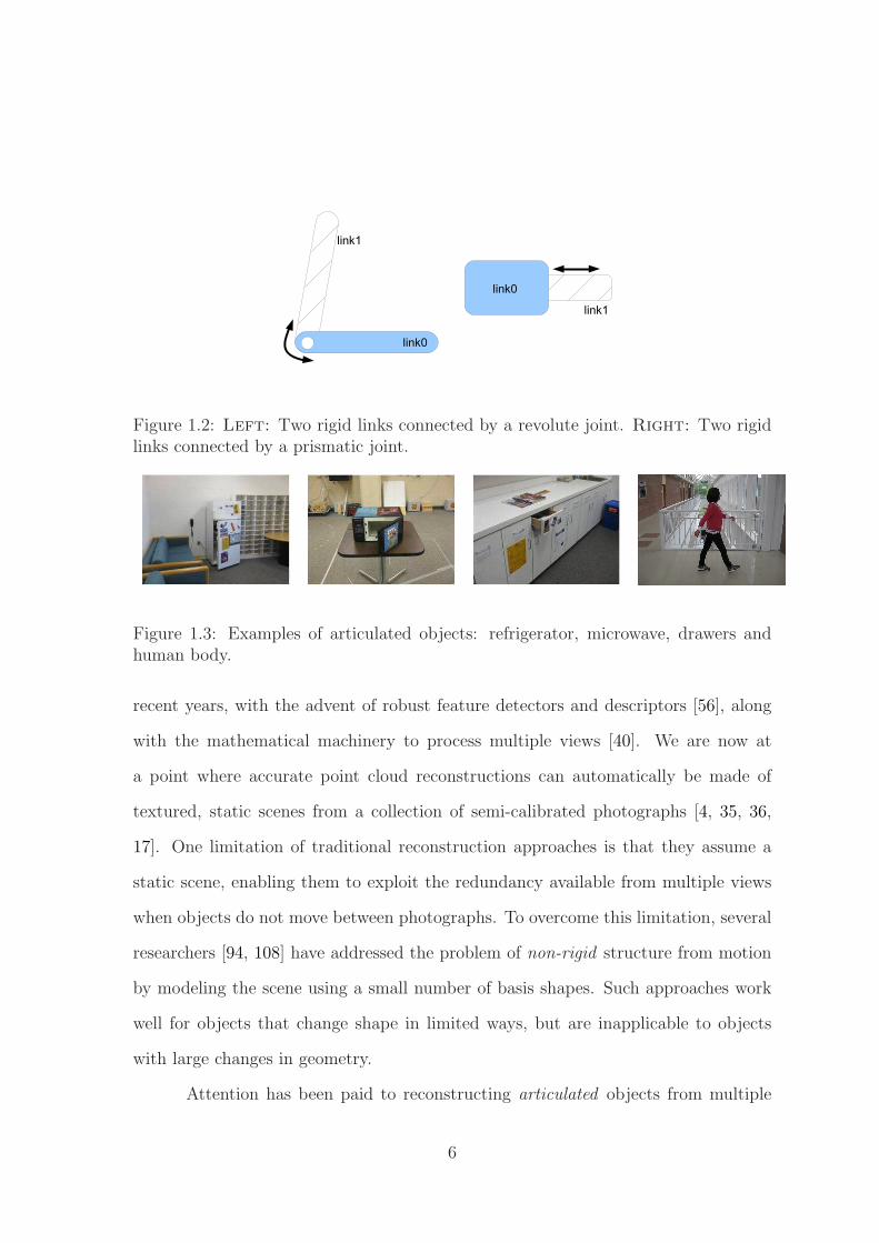
Figure 1.2: Left: Two rigid links connected by a revolute joint. Right: Two rigidlinks connected by a prismatic joint.

Figure 1.3: Examples of articulated objects: refrigerator, microwave, drawers andhuman body.

recent years, with the advent of robust feature detectors and descriptors [56], along

with the mathematical machinery to process multiple views [40]. We are now at

a point where accurate point cloud reconstructions can automatically be made of

textured, static scenes from a collection of semi-calibrated photographs [4, 35, 36,

17]. One limitation of traditional reconstruction approaches is that they assume a

static scene, enabling them to exploit the redundancy available from multiple views

when objects do not move between photographs. To overcome this limitation, several

researchers [94, 108] have addressed the problem of non-rigid structure from motion

by modeling the scene using a small number of basis shapes. Such approaches work

well for objects that change shape in limited ways, but are inapplicable to objects

with large changes in geometry.

Attention has been paid to reconstructing articulated objects from multiple

6

images [110, 80, 48, 90, 67] recently. Approaches to recovering articulated objects

have focused primarily on either human pose recovery from a known skeletal model

or estimation of joint positions from video. These approaches generally do not take

full advantage of multi-view geometry, relying instead upon a known model or affine

projection, and therefore do not reconstruct the surface of the articulated object in

3D. Moreover current approaches to articulated object reconstruction are limited to

a single view. By tracking feature points throughout a video sequence, clustering

the feature points, enforcing noise-robust models, and triangulating the rays, the 3D

coordinates of the features points, as well as the parameters of the joint axes, can

be recovered using any of several techniques. Such approaches, however, do not yield

any information about the back side of the object that is not visible in the current

view. In situations in which the robot wishes to manipulate or interact with such

non-visible portions of the object, a single-view model is not sufficient.

We introduce the term occlusion aware to refer to the robot’s knowledge of

parts of the object that are not visible in the current view. This novel way of ap-

proaching the problem is motivated by recent developments in the structure from

motion community, which has developed fully automated methods capable of recon-

structing complete 3D models from a collection of images [86, 35, 32, 100]. That is,

such methods reconstruct the 3D locations of points on all sides of the object, using

only images from one or several cameras. Such knowledge has always been assumed

in the context of grasping research based on 3D CAD models [6, 51, 65]. However, in

a scenario in which the robot is interactively learning about the unknown objects in

the scene, such models are not available; a new approach is needed.

In this work, we first present an occlusion-aware system for reconstructing

articulated objects from images taken by a camera from different viewpoints. The

proposed method, called Procrustes-Lo-RANSAC, or PLR, first builds two complete

7

3D point cloud models by applying structure-from-motion algorithms to images cap-

tured of the object in two different configurations. Then the method uses Procrustes

analysis combined with a locally optimized RANSAC sampling strategy to auto-

matically segment the points into the individual links. After aligning the links, the

articulated structure of the object is estimated using a geometric approach. Second,

with hand-eye calibration, the robot can align its coordinate system with that of the

recovered articulated model and then manipulate the object by exercising the degrees

of freedom captured by the model. The proposed approach, based on our earlier work

in [43], does not have the limitations of previous systems, in that it uses perspective

projection and does not make any planar assumptions about the scene. We show the

results of the system on a variety of everyday objects, demonstrating the effectiveness

of the approach. Third, a RGBD sensor, Microsoft Kinect, is introduced to improve

the proposed approach by reconstructing high quality 3D articulated models using

KinectFusion algorithm and the geometric approach. With such improvements, the

system yields much denser models and increases the computation efficiency.

1.3 Outline of dissertation

The main goal of the work is to develop algorithms using multiple views to

recover complete 3D models of articulated objects in domestic environments and

thereby enable a robotic system to manipulate objects. The dissertation is organized

in the following manner. Chapter 1 is the introduction of this work. Following the

introduction a summary of the related work in three areas: multi-view reconstruction,

articulated structure and object manipulation is described in Chapter 2. Chapter 3

presents the details of the proposed novel Procrustes-Lo-RANSAC (PLR) algorithm

and demonstrates its performance for a variety of everyday objects. Once the algo-

8

rithm is addressed, its applications to a robotic system and the experimental results

are described in Chapter 4. Chapter 5 begins by describing how to further improve

the previous proposed approach of articulated objects reconstruction in Chapter 3,

then addresses one possible solution which use a RGBD sensor (Microsoft Kinect) to

recover high quality 3D articulated models. Finally conclusions, contributions of this

work and some potential directions for future work are presented in Chapter 6.

9

Chapter 2

Related Work

Reconstruction and manipulation of articulated objects has become an active

area in the computer vision and robotics community in recent years. There are

a number of techniques and progress described in the literature. In the following

sections, we present the related work from three aspects: multi-view reconstruction,

articulated structure and object manipulation.

2.1 Multi-view reconstruction

In generally, multi-view reconstruction techniques use a sequence of images

of an object or a scene from different viewpoints to recover its 3D structure [77].

Recently, many methods have been proposed by researchers in the computer vision

and robotics community to handle various types of datasets either single or clustered

objects, static or dynamic objects, and indoor or outdoor scenes. Most existing

approaches can be categorized into the following two classes in terms of the scene

representation.

10

2.1.1 Point cloud-based approaches

Structure from motion (SFM), in which the 3D point cloud of a scene is esti-

mated by backprojecting corresponding points from multiple images into space, is a

classic problem in computer vision. One approach is to exploit the so-called rank con-

straint to effectively factorize a matrix containing feature coordinates into matrices

containing the shape of the scene and motion of the camera [92]. This factorization

method was later extended to handle not only orthographic cameras but also parap-

erspective [71] projection and multiple bodies [16]. This latter work, by discovering

the block diagonal structure of the measurement matrix in order to segment and re-

construct the geometry of multiple objects, is closely related to this work in terms of

its overall goal.

More recent approaches to structure from motion have abandoned the batch

processing approach of factorization in favor of a pipeline in which pairs of images

are matched sequentially in order to build the 3D reconstruction. In one of the

first approaches to exploit the impressive amount of data available in Community

Photo Collections (CPCs), Snavely et al.[86] combine feature correspondences and an

optimization routine to recover the 3D positions of the features along with the camera

parameters. Goesele et al.[36] describe an approach which takes as input sparse 3D

points from an SFM algorithm (such as the previous) and iteratively grows surfaces

in order to reconstruct the geometry of the scene. Agarwal et al.[4] expanded these

previous systems to handle a million images using a parallel distributed matching

approach and bundle adjustment improvements aimed at minimizing equations with

large numbers of variables. The approaches of Brown and Lowe [11], Sinha and

Pollefeys [81], and Furukawa and Ponce [35] are focused on similar problems with

more limited datasets. All of this work has been concentrated on static scenes, with

11

moving objects (such as tourists in the photos) considered noise to be removed.

A series of papers by Bregler and colleagues addressed the problem of non-

rigid scene reconstruction. In their early work, Bregler et al.[9] showed that 3D

reconstruction of non-rigid objects could be performed by modeling the object using

a set of basis shapes. In follow-up work, Torresani et al.[95] incorporated feature

tracking into the algorithm, so that the resulting system simultaneously solves for

feature tracks, camera pose, and 3D non-rigid structure. Torresani and Bregler [93]

then were able to apply this concept of basis shapes to derive a space-time rank

constraint that results in more robust feature tracking when objects are non-rigid. In

[94], the authors improve upon the earlier reconstruction algorithm by introducing

learned shape priors to overcome ambiguities inherent in the original formulation.

An alternative approach is proposed by Xiao et al.[108] who augmented the rotation

constraints of the previous methods with basis constraints to uniquely determine the

shape bases. Other related work is that of [70], who used a known model of a non-rigid

object not to reconstruct the geometry but rather to detect the object and register it

with the image.

2.1.2 Volume-based approaches

Similar to the pixel, the voxel is a volumetric method to represent visual scene

in three dimensional world. The earliest approach based on volumetric representation

to reconstruct 3D structures of a scene is the visual hull [55, 57]. The visual hull of

an object is formed by intersecting projected silhouettes of the object from different

views. The visual hull provides only the approximate shape of the object. Figure 2.1

shows a 2D example of the visual hull. Typically, the approach based on visual hull

assumes that the foreground object in the collection of images is segmentable from

12

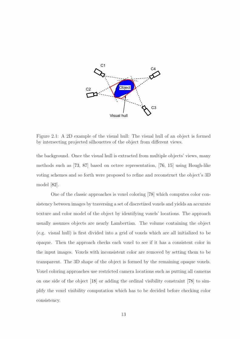
Figure 2.1: A 2D example of the visual hull: The visual hull of an object is formedby intersecting projected silhouettes of the object from different views.

the background. Once the visual hull is extracted from multiple objects’ views, many

methods such as [73, 87] based on octree representation, [76, 15] using Hough-like

voting schemes and so forth were proposed to refine and reconstruct the object’s 3D

model [82].

One of the classic approaches is voxel coloring [78] which computes color con-

sistency between images by traversing a set of discretized voxels and yields an accurate

texture and color model of the object by identifying voxels’ locations. The approach

usually assumes objects are nearly Lambertian. The volume containing the object

(e.g. visual hull) is first divided into a grid of voxels which are all initialized to be

opaque. Then the approach checks each voxel to see if it has a consistent color in

the input images. Voxels with inconsistent color are removed by setting them to be

transparent. The 3D shape of the object is formed by the remaining opaque voxels.

Voxel coloring approaches use restricted camera locations such as putting all cameras

on one side of the object [18] or adding the ordinal visibility constraint [78] to sim-

plify the voxel visibility computation which has to be decided before checking color

consistency.

13

The voxel coloring approach was later extended to handle arbitrary camera

positions by generalized voxel coloring approach [18, 58, 79] and space carving ap-

proach [54, 10]. Unlike voxel coloring approach both approaches scan the voxels

multiple times and check color consistency using updated visibility information. Due

to arbitrary camera locations, projected image pixels of a voxel are not possible to be

visible in all input images [83, 82]. During each carving, both approaches need to find

set of images in which projected image pixels of the voxel are visible. Generalized

voxel coloring approach uses all these images to compute color consistency so that

no voxels with inconsistent color remain in the final model. However space carving

approach only uses part of these images such that the final model may contain voxels

with inconsistent color [18].

More recent approaches based on voxels use level-set or graph-cuts techniques

to optimize the problem of reconstructing 3D object shape. Level-set based methods

[26, 24, 72] formulate the shape of an object in the 3D space as a time-varying implicit

function, then iteratively evolve the geometry of the object by deforming an initial

set of surfaces, and finally recover the object’s shape by solving the zero set of the

function. The latter methods [102, 96, 101, 41, 53] express a 3D object as a discrete

weighted graph which defines a cost function, and extract the shape of the object by

finding the max-flow/min-cut solution of the graph.

Traditional approaches of reconstructing objects from multiple images is lim-

ited by assuming objects do not move between photographs or change shape in limited

ways. Such approaches are inapplicable to articulated objects with large changes in

geometry. Therefore a new approach is needed. We take full advantage of multi-

view reconstruction technique to interactively learn the structure of the unknown

articulated object in 3D instead of relying upon a known model.

14

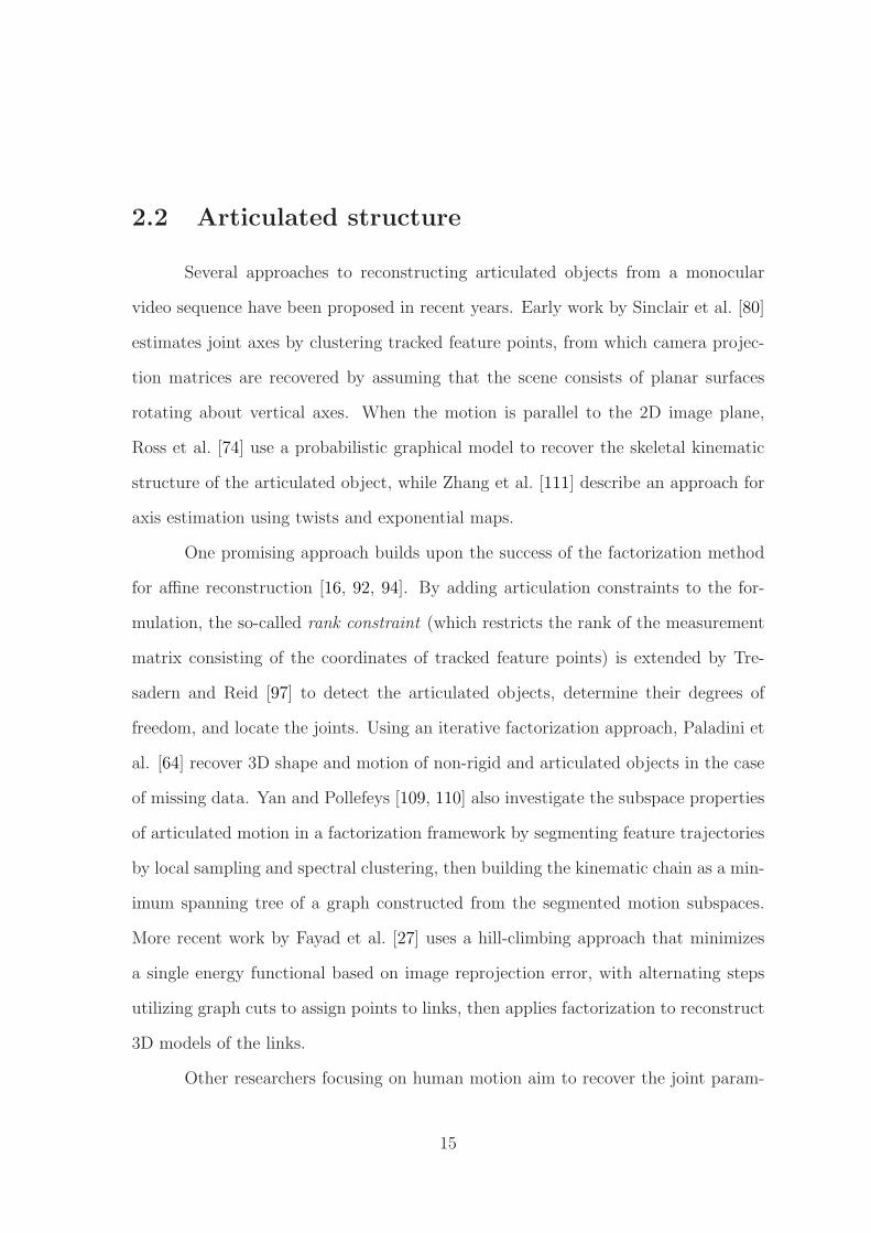
2.2 Articulated structure

Several approaches to reconstructing articulated objects from a monocular

video sequence have been proposed in recent years. Early work by Sinclair et al. [80]

estimates joint axes by clustering tracked feature points, from which camera projec-

tion matrices are recovered by assuming that the scene consists of planar surfaces

rotating about vertical axes. When the motion is parallel to the 2D image plane,

Ross et al. [74] use a probabilistic graphical model to recover the skeletal kinematic

structure of the articulated object, while Zhang et al. [111] describe an approach for

axis estimation using twists and exponential maps.

One promising approach builds upon the success of the factorization method

for affine reconstruction [16, 92, 94]. By adding articulation constraints to the for-

mulation, the so-called rank constraint (which restricts the rank of the measurement

matrix consisting of the coordinates of tracked feature points) is extended by Tre-

sadern and Reid [97] to detect the articulated objects, determine their degrees of

freedom, and locate the joints. Using an iterative factorization approach, Paladini et

al. [64] recover 3D shape and motion of non-rigid and articulated objects in the case

of missing data. Yan and Pollefeys [109, 110] also investigate the subspace properties

of articulated motion in a factorization framework by segmenting feature trajectories

by local sampling and spectral clustering, then building the kinematic chain as a min-

imum spanning tree of a graph constructed from the segmented motion subspaces.

More recent work by Fayad et al. [27] uses a hill-climbing approach that minimizes

a single energy functional based on image reprojection error, with alternating steps

utilizing graph cuts to assign points to links, then applies factorization to reconstruct

3D models of the links.

Other researchers focusing on human motion aim to recover the joint param-

15

eters of the human from video or motion capture [30, 38, 50, 63, 84]. Guan et al. [38]

interactively recover the 3D shape and pose of a human from a single image using

a previously learned model of the human body. Balan et al. [12] optimize a search

over body shape and pose, where the shape is represented as a mesh and fitted using

a graphics model learned off-line from a dataset of detailed 3D range scans of peo-

ple. Freifeld et al. [31] propose a computationally efficient 2D model of a person’s

contour to bridge the gap between 2D and 3D techniques in order to segment human

bodies from images. Forsyth et al. [30] address the problem of tracking articulated

objects, namely humans, in video. Ross et al. [74] model the relationships between

feature point locations on articulated objects as stick figures with fixed lengths and

connectivities. Other approaches to human skeletal tracking include [84, 50, 67].

Research that is most closely related to ours involves reconstructing articu-

lated objects with unknown skeletal parameters. Sturm et al. [91] recover kinematic

models of 1-DOF articulated objects such as microwave ovens by tracking the poses

and orientations of rigid parts captured by the PhaseSpace motion capture system

and addressing a mixture of parameterized and parameter-free (Gaussian process)

representations to best explain the given observation. In related work, the same re-

searchers [90] proposed an approach to learn articulation models of objects without

using artificial markers. Rectangles in depth images obtained from a self-developed

active stereo system are detected using a sampling-based approach. Then the robot

uses generative models learned for the objects to estimate the type of articulation

(revolute or prismatic). In contrast to their work, the proposed approach is not re-

stricted to planar objects. Similar work by Katz et al. [48] reconstructs 3D kinematic

structures of rigid articulated bodies in a single-view and sparse model based on fea-

ture tracking, motion segmentation and classical structure from motion techniques.

In their latest work [46], Katz et al. segment, track and model articulated objects

16

with sufficient texture by using a RGBD sensor so that their approach can handle

partial occlusions and small object motions.

2.3 Object manipulation

Using scene exploration with embedded sensors to reconstruct and manipulate

a 3D model of unknown objects is an approach taken by several researchers [6, 52, 103,

75, 59]. Walck et al. [103] propose a method which automatically finds the position

of the targeted object using a single eye-in-hand camera, captures multiple views

of its shape using visual servoing, and models unknown objects using carved visual

hull techniques. Bone et al. [6] model 3D objects by combining a silhouette model

from a video camera with structured-light model from a laser projector. Klingbeil et

al. [52] address the problem of opening new doors, avoiding the need to reconstruct

3D models by instead detecting door handles and extracting a small number of 3D

features for alignment.

Surveying this literature, there remains a need in the robotics community

to develop techniques to reconstruct 3D models of articulated objects, particularly

models that incorporate the non-visible portions of the objects for occlusion-aware

sensing and manipulation.

17

Chapter 3

Learning Articulated Objects

Figure 3.1 shows an overview of the system presented in this dissertation.

First, a set of images is captured by a camera of the object from different viewpoints

while the object remains stationary. Structure-from-motion techniques are used to

the images to build a 3D model of the object. In order to learn the object’s kinematic

structure, the configuration of the object is interactively changed by exercising its

degrees of freedom. Additional images are gathered of the object in the new configu-

ration, and structure-from-motion yields a different 3D reconstruction. These two 3D

models are segmented into the object’s constituent components (rigid links) using the

proposed Procrustes-Lo-RANSAC (PLR) method. A geometric approach utilizing an

axis-angle representation is then used to estimate the axis of each joint. Based on

these models, the robot with eye-in-hand can automatically compute the transforma-

tion between the object and robot coordinate systems, enabling it to manipulate the

object around the articulation axis with a given grasp point, as shown in Figure 3.2.

We assume that the capability of performing sufficient exploratory interaction

with the object to change its configuration is present. In this way, the approach bears

some resemblance to interactive perception [45, 48, 105, 106, 107], except that we al-

18

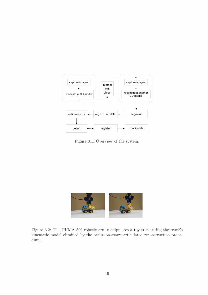
Figure 3.1: Overview of the system.

Figure 3.2: The PUMA 500 robotic arm manipulates a toy truck using the truck’skinematic model obtained by the occlusion-aware articulated reconstruction proce-dure.

19

low either a human or robot to perform the interaction due to the specific constraints

of articulated motion in the objects. Automatically planning the end effector motion

path for interactive perception in such situations remains an unsolved problem, be-

cause a preliminary model (at least) is needed in order to interact with the object,

but the interaction is necessary to estimate the model. Therefore, having the user

perform the interaction enables us to escape this difficult chicken-and-egg problem.

As progress is made toward developing such autonomous exploratory behavior, the

reconstruction method described in this paper still applies.

3.1 Building initial 3D model

We assume the object is a set of rigid links connected by revolute or prismatic

joints, so that a configuration refers to a specific set of values for the joint angles or

displacements. To reconstruct the 3D structure of an articulated object, we capture a

set of images about the object from different camera viewpoints. This work does not

require information about the camera location, orientation, or intrinsic parameters.

Instead, the Bundler Structure from Motion (SfM) package [85, 86] is used to compute

the camera parameters and projection matrices by matching key points. Bundler

extracts focal length, image size, and other information from the EXIF tags of images,

which is embedded by most consumer-level digital cameras. By assuming that the

principal point is near the center of the image, Bundler then uses photo-consistency

and the bundle adjustment algorithm to iteratively compute the desired parameters

in order to minimize the reprojection error. Figure 3.3 shows the 3D models with

camera locations of a toy truck in two different configurations by Bundler.

Once the cameras are calibrated, we apply the patch-based multi-view stereo

(PMVS) algorithm [33, 34] to reconstruct dense 3D oriented points, where each point

20

Figure 3.3: Top: Four images (out of 121 captured) of a toy truck, and the 3D modelwith all camera locations (red points) obtained by Bundler. Bottom: Four images(out of 147 captured) of the truck in a different configuration, along with the 3Dmodel and camera positions (red points).

has an associated 3D location, surface normal, and a set of visible images. Taking

calibrated images and camera parameters as inputs, PMVS begins with a sparse set of

matched features and repeatedly expands the initial matches to nearby pixels, using

visibility constraints to filter out false matches.

This procedure is then repeated to produce a second 3D model from another

set of images obtained of the object in a different configuration in which all adjacent

links have moved relative to each other. Note that only two configurations are needed,

no matter how many links and joints. Figure 3.4 shows the dense 3D reconstruction

of a toy truck in two different configurations. There is no constraint on the set of

images, except that there must be sufficient overlap in the fields of view in order to

facilitate feature matching across different views. In the experience, successive camera

viewpoints should differ by no more than about 10 degrees, so that approximately 36

images are needed to capture an accurate 360-degree model; more images are needed

to reconstruct the top or bottom of the object.

21

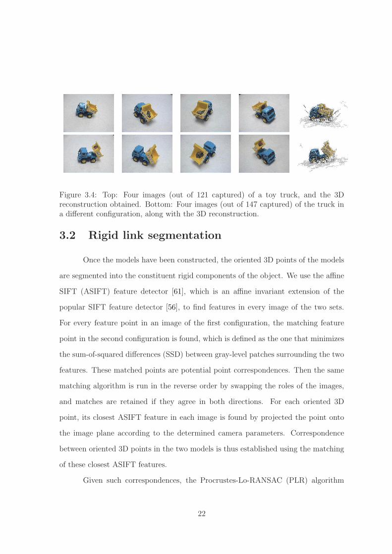
Figure 3.4: Top: Four images (out of 121 captured) of a toy truck, and the 3Dreconstruction obtained. Bottom: Four images (out of 147 captured) of the truck ina different configuration, along with the 3D reconstruction.

3.2 Rigid link segmentation

Once the models have been constructed, the oriented 3D points of the models

are segmented into the constituent rigid components of the object. We use the affine

SIFT (ASIFT) feature detector [61], which is an affine invariant extension of the

popular SIFT feature detector [56], to find features in every image of the two sets.

For every feature point in an image of the first configuration, the matching feature

point in the second configuration is found, which is defined as the one that minimizes

the sum-of-squared differences (SSD) between gray-level patches surrounding the two

features. These matched points are potential point correspondences. Then the same

matching algorithm is run in the reverse order by swapping the roles of the images,

and matches are retained if they agree in both directions. For each oriented 3D

point, its closest ASIFT feature in each image is found by projected the point onto

the image plane according to the determined camera parameters. Correspondence

between oriented 3D points in the two models is thus established using the matching

of these closest ASIFT features.

Given such correspondences, the Procrustes-Lo-RANSAC (PLR) algorithm

22

shown in Algorithm 1 is applied. The first part of this algorithm is motion segmenta-

tion shown in Algorithm 2. Procrustes analysis [25] is run iteratively in combination

with a locally optimized RANSAC (Lo-RANSAC) sampling strategy [14] to find sim-

ilarity transformations of rigid parts. Similarity transformations include rotation,

translation, and scale, where the latter is needed because of the scale ambiguity in

images.

The Procrustes algorithm is a classic method for aligning two point sets [25].

Let X = [x1, . . . ,xn ] and Y = [y1, . . . ,yn ] be two point sets, where each matrix has

dimensions d × n for dimensionality d. (Normally d = 3, but for a 2D scene d = 2.)

First we compute the centroid of each:

µX =1

n

n∑

i=1

xi (3.1)

µY =1

n

n∑

i=1

yi. (3.2)

Scale is handled by normalizing the coordinates using the Frobenius norm:

fX =√

Tr(XXT ), (3.3)

and similarly for fY , where Tr is the trace of the matrix and

X = X − µX1Tn . (3.4)

The scaled, shifted coordinates

X = (X − µX1Tn )/fX (3.5)

Y = (Y − µY 1Tn )/fY , (3.6)

23

where 1n is an n-element vector of all ones, are therefore centered at the origin with

unit scale. The rotation between the point sets is then computed as

R = UΣ′V T , (3.7)

where the singular value decomposition (SVD) of Y XT is UΣV T . Instead of Σ, we use

the matrix Σ′ = diag( 1, 1, det(UV T ) ) to ensure that det(R) = 1, and therefore

that R is a rotation matrix. Putting this all together yields

Y ≈ fYfX

R(X − µX1Tn ) + µY 1

Tn . (3.8)

Given a point xi, then, the similarity transformation is given by σRxi + t, where

σ = fY /fX , and t = −σµX + µY .

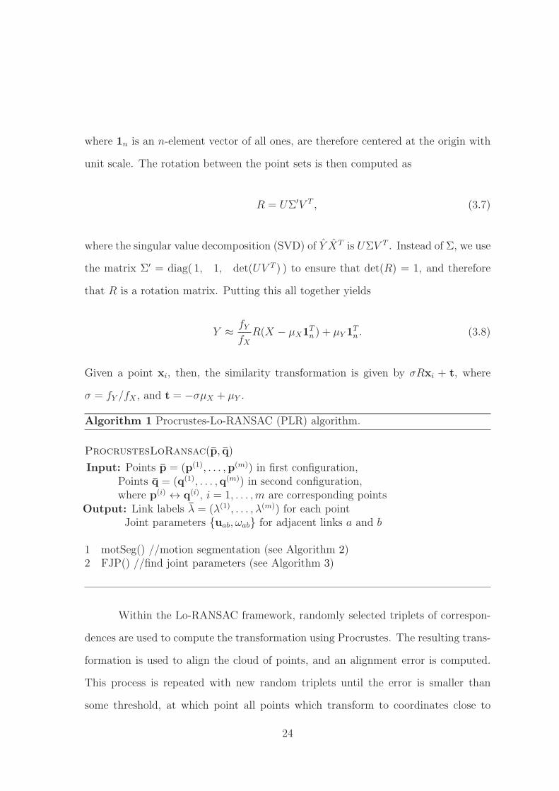
Algorithm 1 Procrustes-Lo-RANSAC (PLR) algorithm.

ProcrustesLoRansac(p, q)

Input: Points p = (p(1), . . . ,p(m)) in first configuration,Points q = (q(1), . . . ,q(m)) in second configuration,where p(i) ↔ q(i), i = 1, . . . ,m are corresponding points

Output: Link labels λ = (λ(1), . . . , λ(m)) for each pointJoint parameters {uab, ωab} for adjacent links a and b

1 motSeg() //motion segmentation (see Algorithm 2)2 FJP() //find joint parameters (see Algorithm 3)

Within the Lo-RANSAC framework, randomly selected triplets of correspon-

dences are used to compute the transformation using Procrustes. The resulting trans-

formation is used to align the cloud of points, and an alignment error is computed.

This process is repeated with new random triplets until the error is smaller than

some threshold, at which point all points which transform to coordinates close to

24

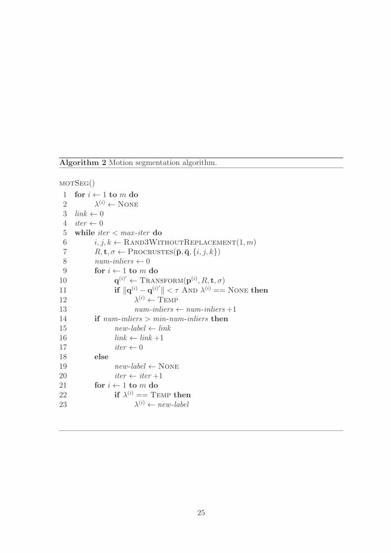
Algorithm 2 Motion segmentation algorithm.

motSeg()

1 for i← 1 to m do2 λ(i) ← None

3 link ← 04 iter ← 05 while iter < max -iter do6 i, j, k ← Rand3WithoutReplacement(1,m)7 R, t, σ ← Procrustes(p, q, {i, j, k})8 num-inliers ← 09 for i← 1 to m do10 q(i)′ ← Transform(p(i), R, t, σ)11 if ‖q(i) − q(i)′‖ < τ And λ(i) == None then12 λ(i) ← Temp

13 num-inliers ← num-inliers +114 if num-inliers > min-num-inliers then15 new -label ← link16 link ← link +117 iter ← 018 else19 new -label ← None

20 iter ← iter +121 for i← 1 to m do22 if λ(i) == Temp then23 λ(i) ← new -label

25

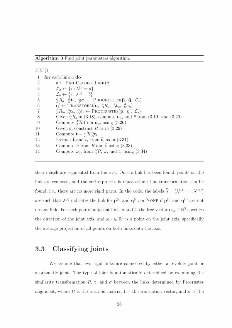
Algorithm 3 Find joint parameters algorithm.

FJP()

1 for each link a do2 b← FindClosestLink(a)3 La ← {i : λ(i) = a}4 Lb ← {i : λ(i) = b}5 A

BRa,ABta,

ABσa ← Procrustes(p, q, La)

6 q′ ← Transform(q, ABRa,

ABta,

ABσa)

7 AARb,

AAtb,

AAσb ← Procrustes(p, q′, Lb)

8 Given AARb in (3.18), compute uab and θ from (3.19) and (3.20)

9 Compute Aπ

AR from uab using (3.26)

10 Given θ, construct R as in (3.29)11 Compute t = Aπ

ARAAtb

12 Extract t and tz from t, as in (3.31)

13 Compute ω from R and t using (3.33)14 Compute ωab from

Aπ

AR, ω, and tz using (3.34)

their match are segmented from the rest. Once a link has been found, points on the

link are removed, and the entire process is repeated until no transformation can be

found, i.e., there are no more rigid parts. In the code, the labels λ = (λ(1), . . . , λ(m))

are such that λ(i) indicates the link for p(i) and q(i), or None if p(i) and q(i) are not

on any link. For each pair of adjacent links a and b, the free vector uab ∈ R3 specifies

the direction of the joint axis, and ωab ∈ R3 is a point on the joint axis, specifically

the average projection of all points on both links onto the axis.

3.3 Classifying joints

We assume that two rigid links are connected by either a revolute joint or

a prismatic joint. The type of joint is automatically determined by examining the

similarity transformation R, t, and σ between the links determined by Procrustes

alignment, where R is the rotation matrix, t is the translation vector, and σ is the

26

relative scaling between the two models. Although one might be inclined to use the

translation vector t to distinguish between the two types of joints, it is important

to note that t will not in general be zero for a revolute joint. This is because the

axis of the coordinate system attached to the link does not necessarily (and usually

will not) align with the axis of rotation. In other words, although we are interested

in rotation about the axis, Procrustes computes the rotation about the origin of

the coordinate system, which is somewhat arbitrarily determined by structure-from-

motion. While these rotations themselves are identical, a non-zero translation t is

needed to compensate for the misalignment. As a result, we instead determine the

type of joint automatically by examining the rotation matrix R: If R is close to the

identity matrix, then the joint is determined to be a prismatic joint; otherwise it is a

revolute joint. This procedure is repeated for each pair of adjacent links.

3.4 Finding joint axes

We now describe the second part of the PLR method shown in Algorithm 1.

For both revolute and prismatic joints, an axis is a ray in 3D space about or along

which the movement occurs. Locating the axis of a prismatic joint is straightforward:

The unit vector t/‖t‖ yields the direction of motion along the prismatic joint, while

the mean of the points on the second link is used as a point on the axis. Revolute

joints are more complicated.

3.4.1 Two links in 2D with revolute joint

To simplify the problem of estimating the revolute joint parameters, let us

begin with the restricted case of an object consisting of just two links in 2D (d = 2).

Let AP be the set of points on the object in the first configuration, and let BQ be

27

the set of points on the object in the second configuration. The leading superscript

indicates the coordinate frame, either {A} or {B}. The two coordinate frames differ

not only by a Euclidean transformation, but also by an unknown scale, since the

points were acquired by images from a camera.

Let us assume that the first point set has been segmented according to the two

links, called Link 0 and Link 1. This yields AP = AP0 ∪ AP1, whereAPi, i ∈ {0, 1}

is the point set for the ith link in the first configuration. Similarly, for the second

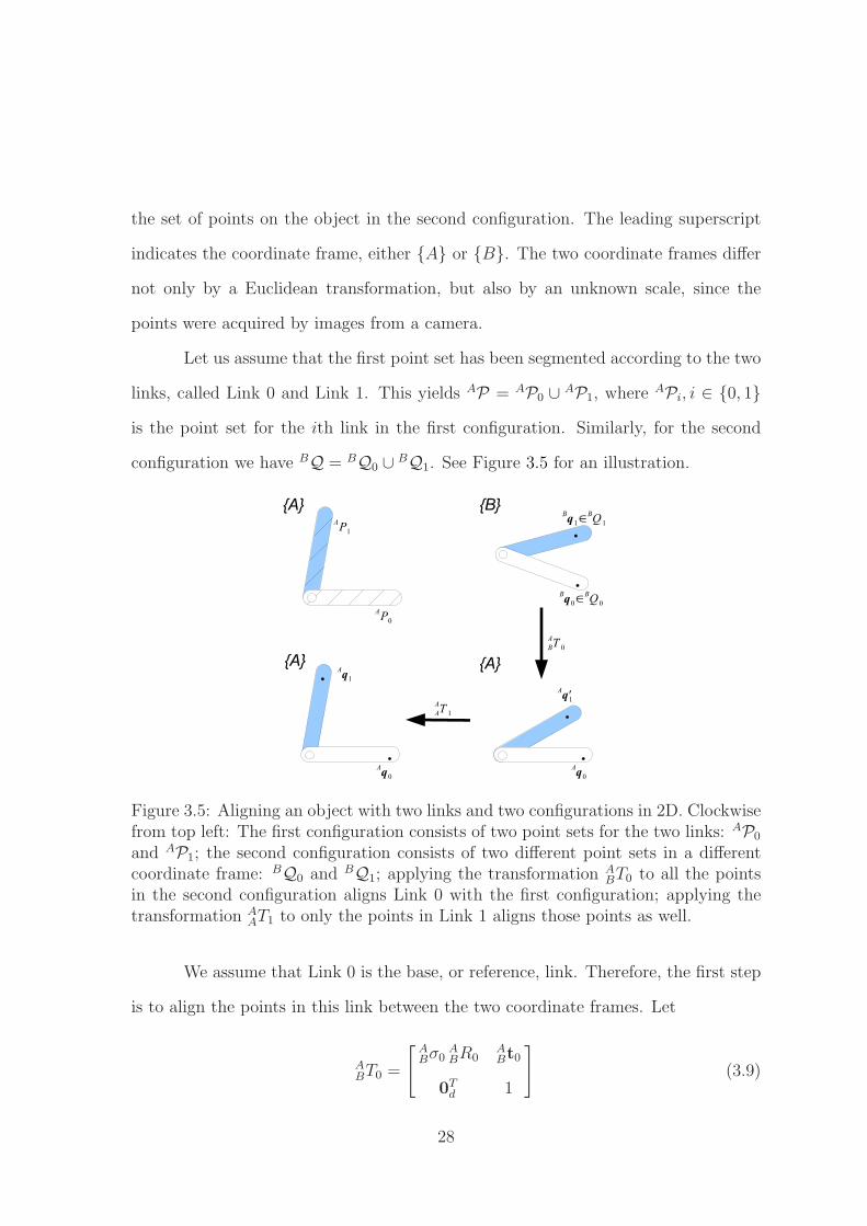
configuration we have BQ = BQ0 ∪ BQ1. See Figure 3.5 for an illustration.

Figure 3.5: Aligning an object with two links and two configurations in 2D. Clockwisefrom top left: The first configuration consists of two point sets for the two links: AP0

and AP1; the second configuration consists of two different point sets in a differentcoordinate frame: BQ0 and BQ1; applying the transformation A

BT0 to all the pointsin the second configuration aligns Link 0 with the first configuration; applying thetransformation A

AT1 to only the points in Link 1 aligns those points as well.

We assume that Link 0 is the base, or reference, link. Therefore, the first step

is to align the points in this link between the two coordinate frames. Let

ABT0 =

[ABσ0

ABR0

ABt0

0Td 1

]

(3.9)

28

be the similarity transformation from coordinate frame {B} to {A} to align Link 0,

where ABR0 is the d× d rotation matrix, A

Bt0 is the d× 1 translation vector, and 0Td is

the transpose of a d × 1 vector of all zeros. Let Bq0 ∈ BQ0 ⊂ Rd be a point in the

second configuration of Link 0, expressed in the second coordinate frame {B}. The

transformation above can be used to express the same point in the first coordinate

frame, {A}:Aq0 =

ABσ0

ABR0

Bq0 +ABt0, (3.10)

or equivalently

Aq0 =ABT0

Bq0, (3.11)

where Bq0 = [(Bq0

)T1 ]T are the homogeneous coordinates of Bq0, and similarly

for Aq0.

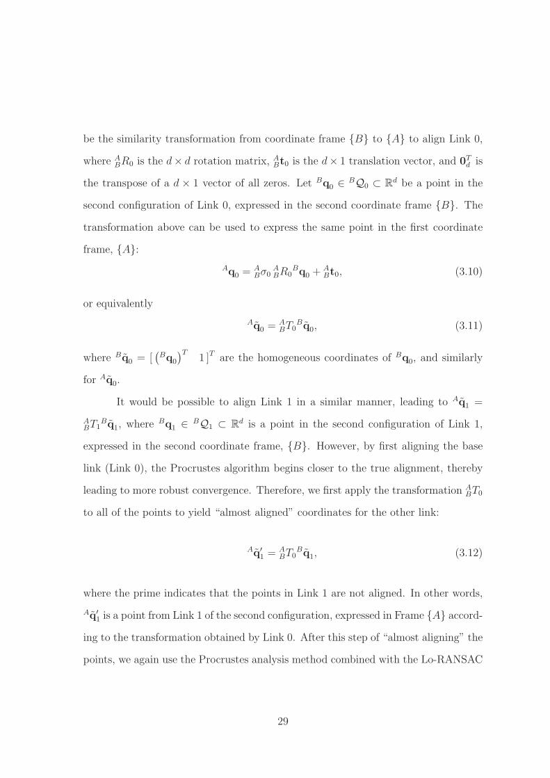
It would be possible to align Link 1 in a similar manner, leading to Aq1 =

ABT1

Bq1, whereBq1 ∈ BQ1 ⊂ R

d is a point in the second configuration of Link 1,

expressed in the second coordinate frame, {B}. However, by first aligning the base

link (Link 0), the Procrustes algorithm begins closer to the true alignment, thereby

leading to more robust convergence. Therefore, we first apply the transformation ABT0

to all of the points to yield “almost aligned” coordinates for the other link:

Aq′

1 =ABT0

Bq1, (3.12)

where the prime indicates that the points in Link 1 are not aligned. In other words,

Aq′

1 is a point from Link 1 of the second configuration, expressed in Frame {A} accord-

ing to the transformation obtained by Link 0. After this step of “almost aligning” the

points, we again use the Procrustes analysis method combined with the Lo-RANSAC

29

sampling strategy to find the transformation AAT1 so that

Aq1 =AAT1

Aq′

1 (3.13)

specifies the coordinates of Link 1 of the second configuration aligned with Link 1

of the first configuration, expressed in Frame {A}. Here the scaling factor should be

equal to 1, so it can safely be ignored. In non-homogeneous coordinates, we have

Aq1 =AAR1

Aq′

1 +AAt1. (3.14)

3.4.2 Finding the 2D axis of rotation

It is a simple matter to show that any Euclidean transformation (rotation plus

translation) can be rewritten as a rotation applied to translated points:

Aq1 = AAR1

Aq′

1 +AAt1 (3.15)

= AAR1

(Aq′

1 − ω)+ ω, (3.16)

where

ω =(Id − A

AR1

)−1 A

At1, (3.17)

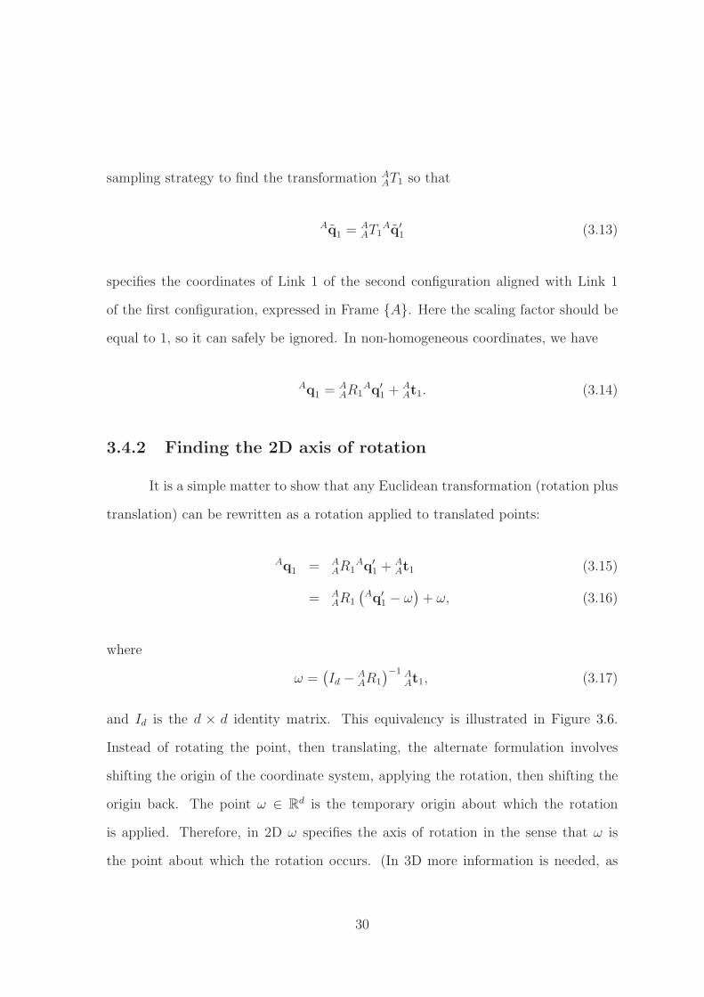
and Id is the d × d identity matrix. This equivalency is illustrated in Figure 3.6.

Instead of rotating the point, then translating, the alternate formulation involves

shifting the origin of the coordinate system, applying the rotation, then shifting the

origin back. The point ω ∈ Rd is the temporary origin about which the rotation

is applied. Therefore, in 2D ω specifies the axis of rotation in the sense that ω is

the point about which the rotation occurs. (In 3D more information is needed, as

30

explained below.)

Figure 3.6: An illustration of the axis of rotation in 2D. Top: Using (3.15), a Eu-clidean transformation involves applying a rotation about the origin, followed by atranslation. Bottom: Using the equivalent expression in (3.16), the transformationinvolves shifting the origin of the coordinate system, then applying the rotation aboutthe temporary origin, then shifting the origin back.

To verify that this equation makes sense, note that in (3.17), the axis of

rotation ω is undefined if AAR1 = Id, i.e., if there is no rotation. Also note that

‖AAt1‖ ≤ 2‖ω‖, which can be seen geometrically because translating by ‖ω‖, then

rotating, then translating again by ‖ω‖ cannot cause a translation of more than 2‖ω‖

as shown in Figure 3.7. Specially, there is no translation when the rotation angle is

zero; the translation ‖AAt1‖ =√2‖ω‖ when the rotation angle is 90 degrees; and the

translation ‖AAt1‖ = 2‖ω‖ when the rotation angle is 180 degrees. Algebraically, the

result follows from the fact that for any n× n unitary matrices U and V (note that

rotation matrices are unitary), ‖U − V ‖ ≤ max{|λU − λV | : λU ∈ LU , λV ∈ LV } if

the right hand side <√2, otherwise ‖U − V ‖ ≤ 2, where LU is the set of eigenvalues

of U , and LV is the set of eigenvalues of V [13]. Also the eigenvalues of I2 are 1 and

1, i.e., (1, 0) and (1, 0) in the complex plane, and the eigenvalues of a 2× 2 rotation

matrix are complex conjugates lying on the unit circle of the complex plane.

31

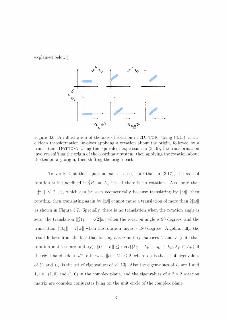
Figure 3.7: An illustration of the translation in 2D: ‖t‖ ≤ 2‖ω‖. Special cases: notranslation if θ = 0; ‖t‖ =

√2‖ω‖ if θ = 90◦; and ‖t‖ = 2‖ω‖ if θ = 180◦ where θ is

the rotation angle.

3.4.3 Extending to 3D

Now we shall extend the two-link case to 3D by letting d = 3. As before, we use

Procrustes analysis combined with Lo-RANSAC to find the Euclidean transformation

ABT0 (now a 3×3 matrix) aligning Link 0 in the second configuration to the same link in

the first configuration. Then the technique is applied again to find the transformation

AAT1 to align Link 1 in the second configuration, where the rotation matrix can be

written as

AAR1 =

r11 r12 r13

r21 r22 r23

r31 r32 r33

. (3.18)

This rotation matrix can be parameterized using the axis-angle representation as a

unit vector u ∈ R3 indicating the direction of a free vector parallel to the axis of

rotation, and an angle θ describing the magnitude of the rotation about the axis in

the right-hand sense. Similarly, the translation AAt1 is parameterized by computing an

arbitrary point ω ∈ R3 on the axis. The rotation angle π ≤ θ ≤ 0 can be computed

32

from the matrix by the simple formula

θ = arccos

(r11 + r22 + r33 − 1

2

)

, (3.19)

where the constraint π ≤ θ ≤ 0 arises from the ambiguity that a rotation of θ about

u is equivalent to a rotation of −θ about −u.

To find the axis u, we note that the eigenvalues of a 3×3 rotation matrix are 1

and cos θ±i sin θ, where i =√−1. Since any vector u parallel to the rotation axis must

remain unchanged by the rotation, the vector must satisfy AAR1u = u. Therefore, from

the definition of eigenvalues and eigenvectors, the axis is the eigenvector corresponding

to the eigenvalue λ = 1. One way to estimate u, then, is to compute the eigenvalues

and eigenvectors of AAR1 and to retain the eigenvector associated with the eigenvalue

of 1. If there is no rotation, i.e., AAR1 = I3, then all three eigenvalues are 1, and the

rotation axis is undefined.

An alternate, simpler formula for computing the axis of rotation is the follow-

ing:

u =u

‖u‖ , where u =

r32 − r23

r13 − r31

r21 − r12

, (3.20)

and ‖ · ‖ is the L2 norm. Note that this formula not only does not work when θ = 0

(in which case the axis is undefined) but also when θ = π (in which case the formula

yields an unhelpful u = [ 0 0 0 ]T ).

Once the axis of rotation u has been found, the 3D rotation about this axis can

be thought of as a 2D rotation in the plane Πu perpendicular to u. Figure 3.8 shows

the vector u in the current coordinate frame {A}. Let us define a new coordinate

frame {Aπ} such that the zπ axis is aligned with u. Therefore, the plane Πu is the

33

same as the xπyπ plane in {Aπ}. To transform from {A} to {Aπ}, we rotate about

the y axis by α, then about the original x axis by β. By geometry (see the figure),

these angles are given by

cosα = uz/η (3.21)

sinα = ux/η (3.22)

cos β = η (3.23)

sin β = uy, (3.24)

where η =√

u2x + u2

z and u = [ ux uy uz ]T . Since the rotation axes are fixed, the

matrices are composed in right-to-left order, yielding an overall transformation of

Aπ

AR =

1 0 0

0 cβ −sβ0 sβ cβ

cα 0 sα

0 1 0

−sα 0 cα

(3.25)

=

uz/η 0 ux/η

uxuy/η η −uyuz/η

−ux uy uz

, (3.26)

where cα = cosα, sα = sinα, and similarly for cβ and sβ.

Now that we have found Aπ

AR, we can apply this rotation matrix to the data to

align the x and y axes with the xπyπ plane, then rotate about the z axis by θ, then

rotate back:

AAR1 =

Aπ

ART

cθ −sθ 0

sθ cθ 0

0 0 1

︸ ︷︷ ︸

Rθz

Aπ

AR (3.27)

34

Figure 3.8: The axis of rotation u is parameterized by angles α and β, and the planeΠu is perpendicular to u.

Including translation, we have

Aq1 = AAR1

Aq′

1 +AAt1

= Aπ

ARTRθ

zAπ

ARAq′

1 +AAt1.

As we noted before, we can rewrite this application of rotation followed by translation

as a shift of the origin, followed by a rotation, followed by a shift back:

Aq1 = Aπ

ARTRθ

zAπ

AR(Aq′

1 − ω)+ ω,

where

ω =(

Id − Aπ

ARTRθ

zAπ

AR)−1

AAt1, (3.28)

where Id is the d × d identity matrix. As before, if Aπ

AR is the identity matrix (no

rotation), then the point ω about which we are rotating is undefined because Id−Rθz

is singular. The point ω is the unique point in 3D where the appropriate 3D rotation

about it aligns Aq′

1 with Aq1.

Although (3.28) should work, we have found better results are obtained by an

alternate approach in which we use a 3D rotation to align the x-y plane with Πu (or

35

equivalently, the z axis with u), then apply the 2D formula in (3.17) to compute ω,

then rotate back. Let us define R as the upper 2× 2 part of Rθz:

R =

[cθ −sθsθ cθ

]

. (3.29)

Define q as the first two elements of Aπ

q′

1 = Aπ

ARAq′

1, and qz as the third element, so

that

Aπ

q′

1 =

[q

qz

]

. (3.30)

Define t as the first two elements of t = Aπ

ARAAt1, and tz as the third element, so that

t =

[t

tz

]

. (3.31)

Now we have

Aq1 =Aπ

ART

([R (q− ω) + ω

qz

]

+

[02

tz

])

, (3.32)

where 02 is a 2× 1 vector of all zeros and

ω =(

I2 − R)−1

t, (3.33)

where I2 is the 2× 2 identity matrix. Once ω is found, the final 3D point ω is given

by

ω = Aπ

ART

[ω

tz

]

. (3.34)

3.5 Experimental results

The performance of the PLR algorithm was evaluated on a variety of different

real-world objects, such as those that might be found in a home, office, or kitchen.

36

Figure 3.9: Axis estimation of the truck. The top two rows show ten images (out of121) of the first configuration, and ten images (out of 147) of the second configuration.The last row shows the estimated axis (red line) overlaid on an image and 3D modelfrom each configuration.

For the experiments, we used a Logitech Quickcam Pro 5000 for collecting images,

mounted on a PUMA 500 robotic arm for manipulation.

We first demonstrate the PLR algorithm on the toy truck encountered earlier.

Figure 3.9 shows some of the images used to reconstruct the two 3D models, along

with the estimated axis overlaid on two of those images and on the 3D models. A

total of 121 and 147 images, respectively, were needed to reconstruct the two models.

Visually, the axis appears to be quite close to the true axis, indicating that the

algorithm was able to accurately segment the links and estimate the position and

orientation of the axis.

The next experiment involved refrigerators. Figure 3.10 shows a synthetic

refrigerator created by the 3D modeling software known as Blender [1]. During the

interaction, 16 images were captured for each configuration respectively. The first

shows two images selected from the two sets overlaid with the axis of rotation (red

line). The 3D reconstructions and estimated rotation axis of rotation are shown in the

figure. Also we demonstrate the result on a real refrigerator, shown in Figure 3.11.

We also tested the approach on more practical items. Figure 3.11 shows the

37

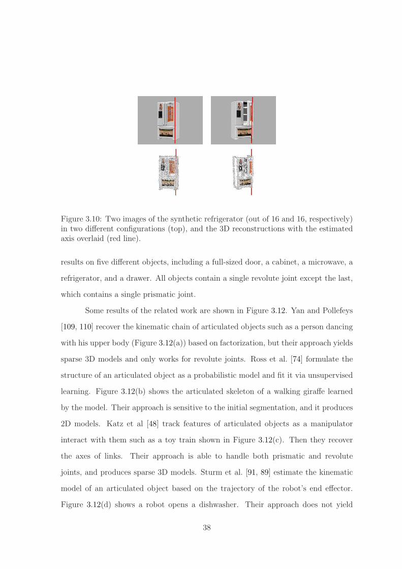
Figure 3.10: Two images of the synthetic refrigerator (out of 16 and 16, respectively)in two different configurations (top), and the 3D reconstructions with the estimatedaxis overlaid (red line).

results on five different objects, including a full-sized door, a cabinet, a microwave, a

refrigerator, and a drawer. All objects contain a single revolute joint except the last,

which contains a single prismatic joint.

Some results of the related work are shown in Figure 3.12. Yan and Pollefeys

[109, 110] recover the kinematic chain of articulated objects such as a person dancing

with his upper body (Figure 3.12(a)) based on factorization, but their approach yields

sparse 3D models and only works for revolute joints. Ross et al. [74] formulate the

structure of an articulated object as a probabilistic model and fit it via unsupervised

learning. Figure 3.12(b) shows the articulated skeleton of a walking giraffe learned

by the model. Their approach is sensitive to the initial segmentation, and it produces

2D models. Katz et al [48] track features of articulated objects as a manipulator

interact with them such as a toy train shown in Figure 3.12(c). Then they recover

the axes of links. Their approach is able to handle both prismatic and revolute

joints, and produces sparse 3D models. Sturm et al. [91, 89] estimate the kinematic

model of an articulated object based on the trajectory of the robot’s end effector.

Figure 3.12(d) shows a robot opens a dishwasher. Their approach does not yield

38

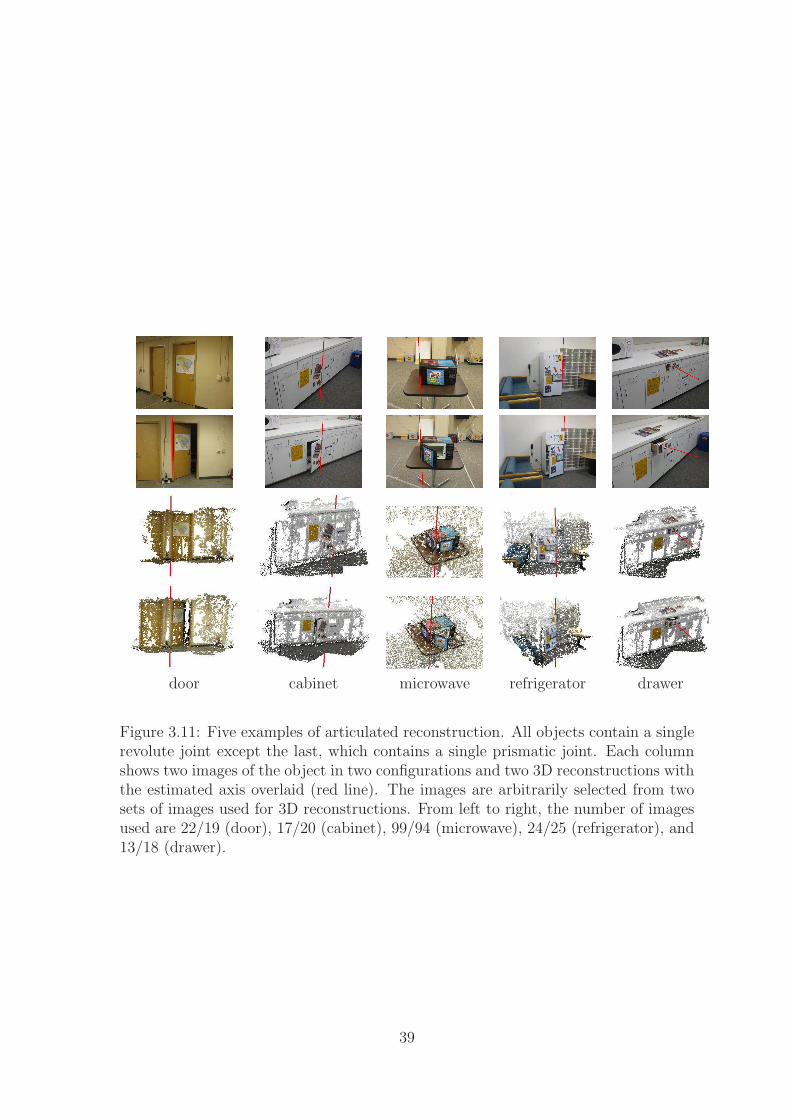
door cabinet microwave refrigerator drawer

Figure 3.11: Five examples of articulated reconstruction. All objects contain a singlerevolute joint except the last, which contains a single prismatic joint. Each columnshows two images of the object in two configurations and two 3D reconstructions withthe estimated axis overlaid (red line). The images are arbitrarily selected from twosets of images used for 3D reconstructions. From left to right, the number of imagesused are 22/19 (door), 17/20 (cabinet), 99/94 (microwave), 24/25 (refrigerator), and13/18 (drawer).

39

(a) (b) (c) (d) (e)

Figure 3.12: Results of related work. (a) The recovered kinematic chain of a persondancing with his upper body in Yan et al. [109, 110]. (b) The estimated articulatedskeleton of a walking giraffe in Ross et al. [74]. (c) Tracking features of a toy train asa manipulator interacts with it in Katz et al. [48]. (d) A robot opens a dishwasher inSturm et al. [91, 89]. (e) The recovered articulation model of a drawer in Sturm etal. [90].

3D models. Also Sturm et al. [90] use an active stereo camera to detect doors and

drawers. Figure 3.12(e) shows the recovered articulation model of a drawer. Their

approach is limited to handle planar objects.

Compared with these work, the proposed method in this work is able to re-

construct fairly dense 3D models, segment the points into the individual links, and

accurately estimate the axis of rotation or translation. Also it supports both revo-

lute and prismatic joints, and does not make any assumptions regarding planarity of

the object. This method automatically classifies joints type and works for objects

with multiple joints. The resulting models therefore include dense 3D point clouds

representing the surfaces of the objects, along with the joint parameters.

To quantify the accuracy of the estimated axes, we computed the angle between

the axis and the normal of a plane in the scene, where the plane was obtained by

fitting plane parameters to points from the cloud corresponding to the real plane in

the scene. For example, in the cases of the door, cabinet, and refrigerator, the floor

plane was obtained, and the error was deemed to be the angle between the estimated

axis and the normal of the floor. For the microwave, truck, and drawer, the same

procedure was followed, except that a plane was fit to the table instead of the floor,

40

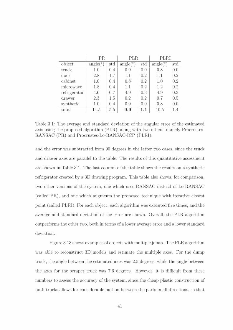
PR PLR PLRIobject angle(◦) std angle(◦) std angle(◦) stdtruck 1.0 0.4 0.9 0.0 0.8 0.0door 2.8 1.7 1.1 0.2 1.1 0.2cabinet 1.0 0.4 0.8 0.2 1.0 0.2microwave 1.8 0.4 1.1 0.2 1.2 0.2refrigerator 4.6 0.7 4.9 0.3 4.9 0.3drawer 2.3 1.5 0.2 0.2 0.7 0.5synthetic 1.0 0.4 0.9 0.0 0.8 0.0total 14.5 5.5 9.9 1.1 10.5 1.4

Table 3.1: The average and standard deviation of the angular error of the estimatedaxis using the proposed algorithm (PLR), along with two others, namely Procrustes-RANSAC (PR) and Procrustes-Lo-RANSAC-ICP (PLRI).

and the error was subtracted from 90 degrees in the latter two cases, since the truck

and drawer axes are parallel to the table. The results of this quantitative assessment

are shown in Table 3.1. The last column of the table shows the results on a synthetic

refrigerator created by a 3D drawing program. This table also shows, for comparison,

two other versions of the system, one which uses RANSAC instead of Lo-RANSAC

(called PR), and one which augments the proposed technique with iterative closest

point (called PLRI). For each object, each algorithm was executed five times, and the

average and standard deviation of the error are shown. Overall, the PLR algorithm

outperforms the other two, both in terms of a lower average error and a lower standard

deviation.

Figure 3.13 shows examples of objects with multiple joints. The PLR algorithm

was able to reconstruct 3D models and estimate the multiple axes. For the dump

truck, the angle between the estimated axes was 2.5 degrees, while the angle between

the axes for the scraper truck was 7.6 degrees. However, it is difficult from these

numbers to assess the accuracy of the system, since the cheap plastic construction of

both trucks allows for considerable motion between the parts in all directions, so that

41

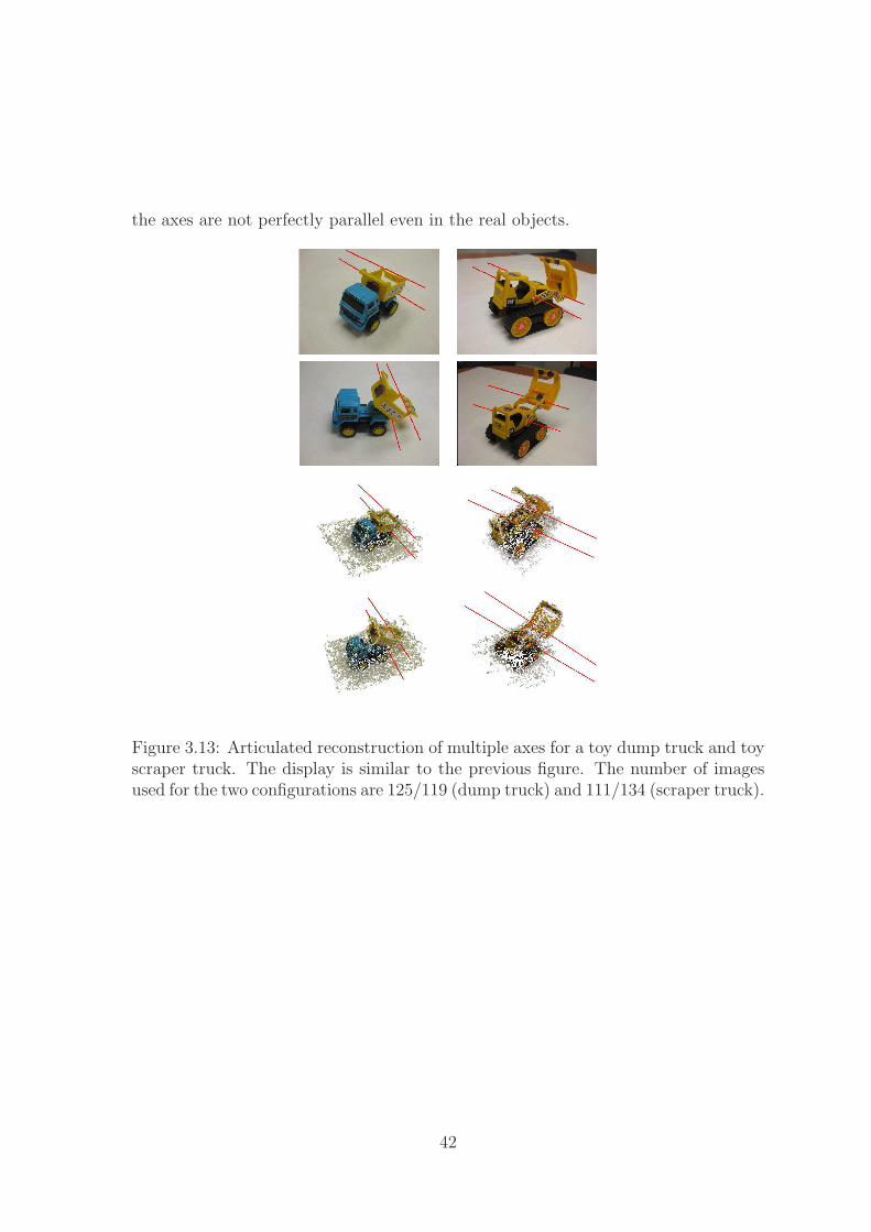
the axes are not perfectly parallel even in the real objects.

Figure 3.13: Articulated reconstruction of multiple axes for a toy dump truck and toyscraper truck. The display is similar to the previous figure. The number of imagesused for the two configurations are 125/119 (dump truck) and 111/134 (scraper truck).

42

Chapter 4

Manipulating Articulated Objects

Once the occlusion-aware 3D articulated model has been obtained, it can be

used by a robot to manipulate the object. Given a particular point on the object, the

robot can move its end effector to that position, even if the point is not visible in the

current view. This is one of the main advantages of the occlusion-aware approach,

namely, that the robot is not limited only to the side of the object that is currently

visible, but rather that a full 3D model is available. Having grasped the object at a

point, it can then use its knowledge of the articulation axis in order to move in such

a way as to exercise the articulation.

In the robotic manipulation system, we use a PUMA 500 robotic arm and

a handhold digital camera mounted on the robot end-effector hand. The first step

for manipulation is to estimate the transformation between the object model and

the robot coordinate frame. To make this a Euclidean transformation, we first must

overcome the scale (σ) ambiguity. The scale of the object can be estimated in one

of several ways. If the camera is attached to the robot during capture time, then

the known positions of the end effector can be compared with the estimated camera

positions to determine the overall scale of the scene. Alternatively, a separate step

43

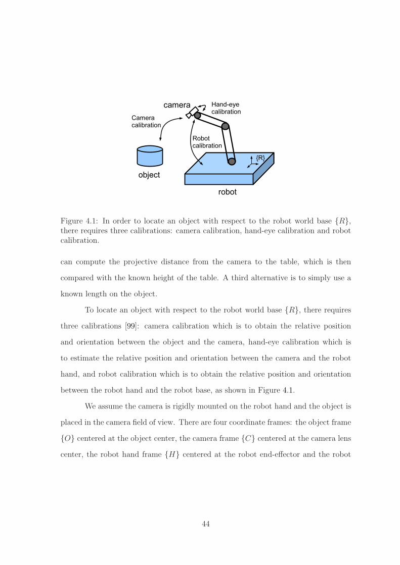
Figure 4.1: In order to locate an object with respect to the robot world base {R},there requires three calibrations: camera calibration, hand-eye calibration and robotcalibration.

can compute the projective distance from the camera to the table, which is then

compared with the known height of the table. A third alternative is to simply use a

known length on the object.

To locate an object with respect to the robot world base {R}, there requires

three calibrations [99]: camera calibration which is to obtain the relative position

and orientation between the object and the camera, hand-eye calibration which is

to estimate the relative position and orientation between the camera and the robot

hand, and robot calibration which is to obtain the relative position and orientation

between the robot hand and the robot base, as shown in Figure 4.1.

We assume the camera is rigidly mounted on the robot hand and the object is

placed in the camera field of view. There are four coordinate frames: the object frame

{O} centered at the object center, the camera frame {C} centered at the camera lens

center, the robot hand frame {H} centered at the robot end-effector and the robot

44

base frame {R} centered at the robot base. Let

COT =

[COR

COt

0 1

]

(4.1)

be the relative pose of the camera with respect to the object frame {O}, where the

leading superscript indicates the frame in which the transformation is and the leading

subscript indicates the frame to which the transformation is relative. Similarly, we

have the relative pose of the camera with respect to the robot hand CHT and the

relative pose of the robot hand with respect to the robot base HRT .

Once above three poses are estimated, the 3D position and orientation of the

object relative to the robot base frame is computed by

ORT = σ C

OT −1 CHT H

RT . (4.2)

Therefore, for any given particular point Op = [X Y Z 1 ]T (in the homogeneous

coordinate) on the object, the robot can locate its end effector to that position using

Rp = ORT Op (4.3)

even if the point is not visible in the current view. Usually the robot kinematic

system provides the relative pose of the robot hand HRT . In the following we describe

hand-eye calibration and object pose estimation in detail.

4.1 Hand-eye calibration

To compute the homogeneous transformation between the camera and the

robot hand, we mount the camera on the robot hand and place a calibration object

45

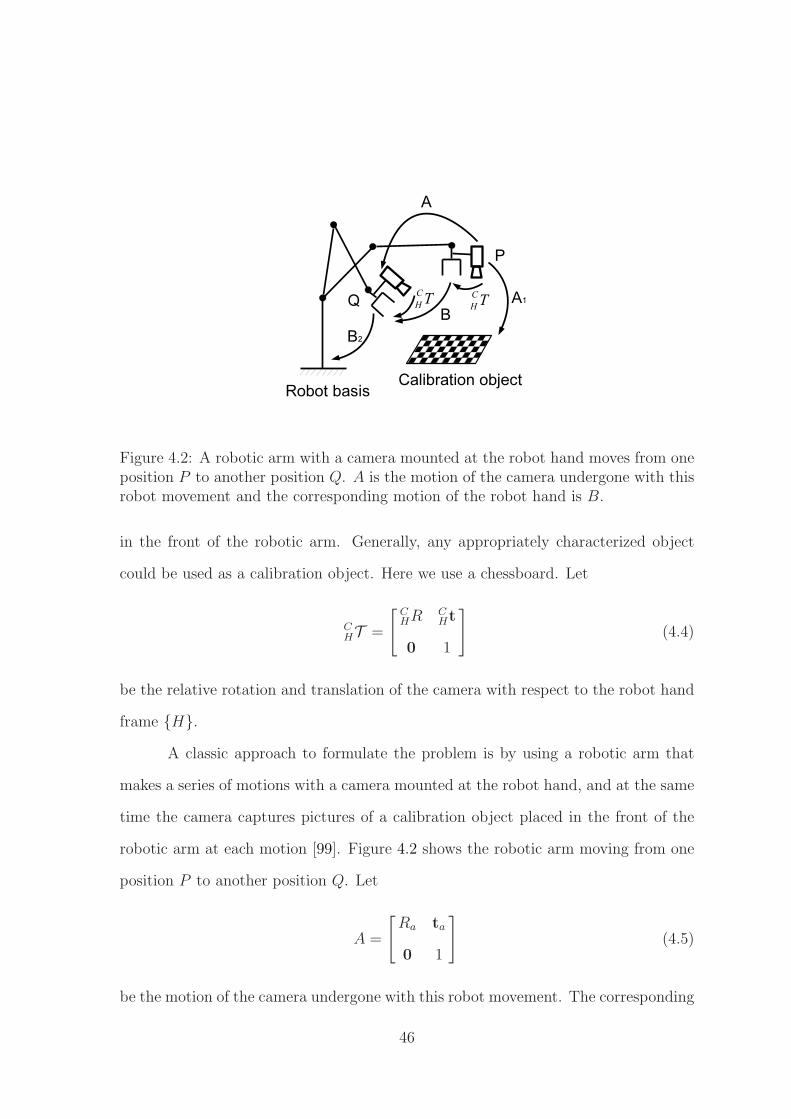
Figure 4.2: A robotic arm with a camera mounted at the robot hand moves from oneposition P to another position Q. A is the motion of the camera undergone with thisrobot movement and the corresponding motion of the robot hand is B.

in the front of the robotic arm. Generally, any appropriately characterized object

could be used as a calibration object. Here we use a chessboard. Let

CHT =

[CHR

CHt

0 1

]

(4.4)

be the relative rotation and translation of the camera with respect to the robot hand

frame {H}.

A classic approach to formulate the problem is by using a robotic arm that

makes a series of motions with a camera mounted at the robot hand, and at the same

time the camera captures pictures of a calibration object placed in the front of the

robotic arm at each motion [99]. Figure 4.2 shows the robotic arm moving from one

position P to another position Q. Let

A =

[Ra ta

0 1

]

(4.5)

be the motion of the camera undergone with this robot movement. The corresponding

46

motion of the robot hand is

B =

[Rb tb

0 1

]

. (4.6)

The two motions are conjugated by the hand-eye transformation CHT [5, 88, 99, 42,

19, 66]. This yields

A CHT = C

HT B (4.7)

where A = A1A−12 and B = B1B

−12 . Ai is the pose of the camera with respect to the

world coordinate system at each motion, and it can be estimated using the camera

extrinsic calibration techniques. Bi is the pose of the robot hand with respect to the

robot base system, that is usually provided by the robot kinematic system. The only

unknown in the equation is CHT . Applied each homogeneous transformation matrix,

(4.7) is split into

RaCHR = C

HR Rb, (4.8)

RaCHt+ ta =

CHR tb +

CHt. (4.9)

Note once CHR in (4.8) is solved, (4.9) can also be solved.

Many methods [5, 88, 99, 42, 19, 66] were proposed by researchers to solve

this homogeneous matrix equation. Tsai and Lenz [99] first decouple the rotational

part from the translation using the screw (angle-axis) representation and solve the

equation using least squares with a closed form solution. The method yields a simple

numerical solution, but its performance is limited by errors of the linear system, the

parameters of the robot kinematic system and the estimations of the camera rotation

and translation [42]. Park and Martin [66] solve the problem using methods of Lie

theory in a similar way to [99], but also deal with the noise presented in the mea-

surements of A and B. Horaud and Dornaika [42] use unit quaternion to present

rotation and also find a closed form solution for rotation and translation simultane-

47

ously by a non-linear technique. In [19] dual quaternions are introduced by Daniilidis

to perform hand-eye calibration. By using the dual-quaternion parameterization and

singular value decomposition (SVD) the proposed method can quickly find a new

simultaneous solution for the hand-eye rotation and translation. Based on Camera

Calibration Toolbox for Matlab [8] and Hand-Eye Calibration Toolbox [104], we esti-

mate the pose of the camera relative to the robot hand using the proposed approaches

by [99, 42, 19, 66].

4.2 Object pose estimation

To estimate the relative pose of the object with respect to the camera mounted

on the robot hand, we place the object in the camera field of view and take an image

of the object at some viewpoint. There are several approaches we can use to estimate

the relative 3D position and orientation of the object. One is perspective n-point

(PNP) algorithm [62, 2], another is the POSIT algorithm [23].

Both approaches require 2D-3D correspondences between the current image

and the 3D model as an input argument. To produce these correspondences, we use

the affine SIFT (ASIFT) feature detector [61] to find features in the current image

and the image sets used for reconstructing the 3D models. For every feature point

in the current image, the matching feature point in the image sets is found, which

is defined as the one that minimizes the sum-of-squared differences (SSD) between

gray-level patches surrounding the two features. These matched points are potential

point correspondences. Then, the same matching algorithm is run in the reverse

order by swapping the roles of the images, and matches are retained if they agree in

both directions. The image with the largest number of matches in the image sets is

then used to produce 2D-3D correspondences between the current image and the 3D

48

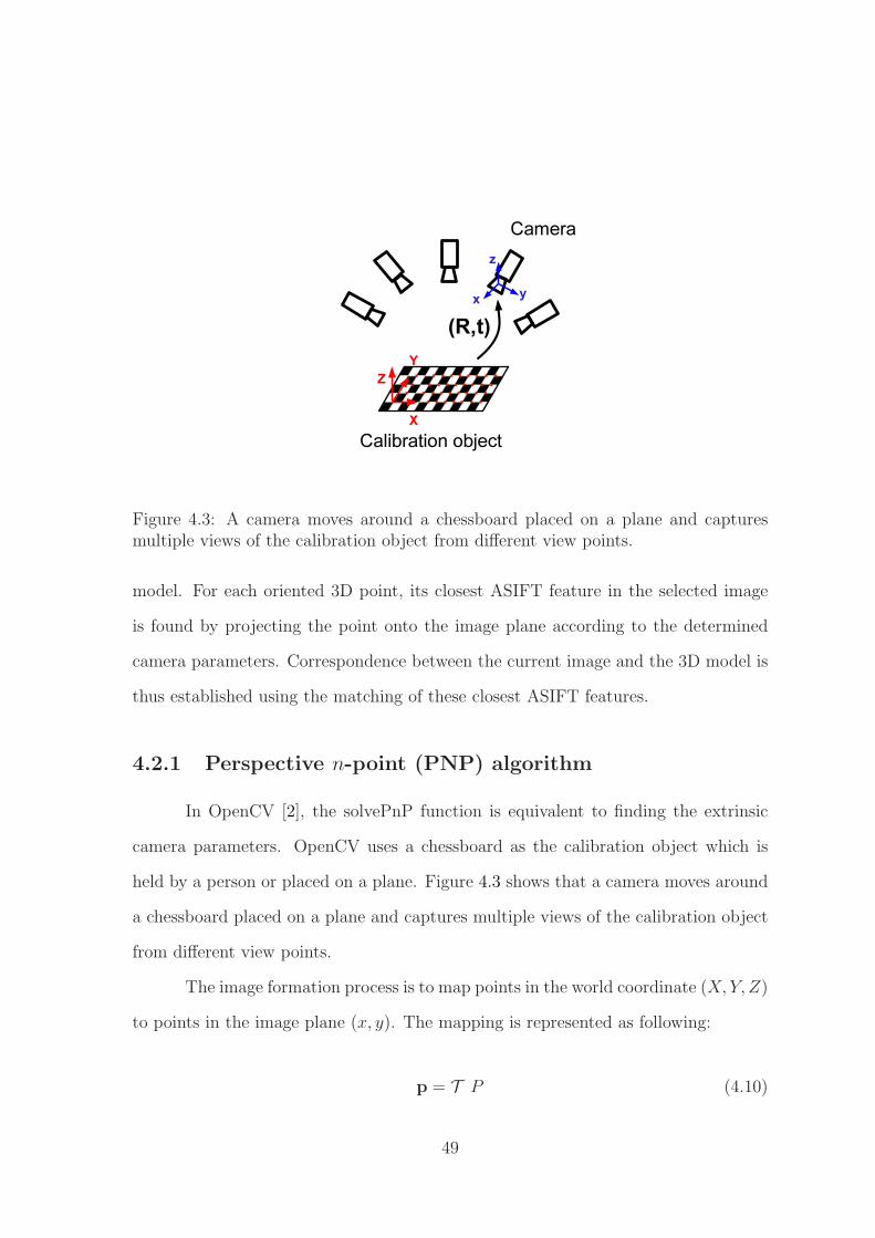
Figure 4.3: A camera moves around a chessboard placed on a plane and capturesmultiple views of the calibration object from different view points.

model. For each oriented 3D point, its closest ASIFT feature in the selected image

is found by projecting the point onto the image plane according to the determined

camera parameters. Correspondence between the current image and the 3D model is

thus established using the matching of these closest ASIFT features.

4.2.1 Perspective n-point (PNP) algorithm

In OpenCV [2], the solvePnP function is equivalent to finding the extrinsic

camera parameters. OpenCV uses a chessboard as the calibration object which is

held by a person or placed on a plane. Figure 4.3 shows that a camera moves around

a chessboard placed on a plane and captures multiple views of the calibration object

from different view points.

The image formation process is to map points in the world coordinate (X, Y, Z)

to points in the image plane (x, y). The mapping is represented as following:

p = T P (4.10)

49

where p = [ x y w ]T , P = [X Y Z W ]T in the homogeneous coordinate and

T =

fx 0 cx

0 fy cy

0 0 1

[R t ] = K D. (4.11)

where K is the camera intrinsic matrix and D is the camera extrinsic matrix. In

general, the camera intrinsics parameters include focal lengths (fx, fy) in pixels along

x and y axes, and a principal point (cx, cy) which is a displacement of the optic

axis away from the center of coordinate on the image plane. The camera extrinsic

parameters are the relative position (t) and orientation (R) of the camera with respect

to the object frame.

In Figure 4.3, the object coordinate is defined so that Z = 0. Applied R =

[ r1 r2 r3 ] and (4.11), (4.10) is rewritten as

p = K [ r1 r2 r3 t ]

X

Y

0

W

, (4.12)

= K [ r1 r2 t ]

X

Y

W

, (4.13)

= H P ′. (4.14)

where H is the homography matrix that maps a planar object’s points onto the im-

age’s points. We assume the camera intrinsics parameters are known (They can be

estimated by the same way with multiple views of the object). For each camera posi-

tion there are six unknowns including three angles for the rotation and three offsets

50

for the translation. To solve H, we at least need 4 pairs of 2D-3D correspondences

which yield eight equations. OpenCV extracts the corners of the chessboard as the

feature points which are shown in Figure 4.3 by red points on the chessboard. In

practice, due to noise of images capturing and errors of numerical calculation, the

more correspondences we use, the better result we get. Once the homography ma-

trix H is solved by linear algebra techniques, the camera extrinsic parameters can

be obtained simultaneously. More details can be found in [112]. We feed the 2D-3D

correspondences to OpenCV solvePnP routine. It turns out that solvePnP works well

for planar objects (chessboards) or near planar objects (human’s faces) due to the

above algorithm OpenCV used.

4.2.2 POSIT algorithm

The POSIT (Pose from Orthography and Scaling with Iterations) algorithm

is to estimate the pose of an object from a single view using at least four or more

feature points [23]. The algorithm does not require the correspondences to be planar.

The approach iteratively approximates the position and orientation of the object

obtained by POS (Pose from Orthography and Scaling) algorithm which simplifies a

perspective projection with a scaled orthographic projection. A scaled orthographic

projection is an orthographic projection followed by a scaling. In Figure 4.4, an object

AB is projected to AB′ by an orthographic projection on a plane Q which is parallel

to the image plane. Then AB′ is projected to ab on the image plane by a perspective

projection. AB′ is scaled down to ab by a scaling factor that is defined by the focal

length and the depth of the object.

Since an object pose can be exactly estimated by the POS algorithm with

feature points on the object and their projected points on the image by a scaled

51

Figure 4.4: Scaled orthographic projection and perspective projection. The scaled or-thographic projection ab of an object AB is the orthographic projection AB′ followedby a scaling. ad is the perspective projection of the object AB.

orthographic projection (SOP), the POSIT algorithm first assumes that the given

image points are projected by a SOP instead of by a perspective projection. Then

the POS algorithm is applied to these points and an approximate pose of the object

is obtained. Next, the feature points and the SOP image are updated by the ap-

proximate pose. Then the POS algorithm is applied to the new SOP image again to

improve SOP image points. These steps are repeated until an accurate object pose is

found.

Alternative approaches include the proposed algorithm in [22] and the Soft-

POSIT algorithm [20]. DeMenthon and Davis [22] introduce nonlinear terms in the

perspective projection model of an object. Additional image uncertainty about these

nonlinear terms can be obtained in two 4D spaces by linear constraints, which leads to

high-order complexity of algorithm performance. Then binary tree search techniques

are used to find the object pose. The SoftPOSIT algorithm computes correspondences

between feature points on the object and their image points when they are unknown

52

using the iterative softassign algorithm [37], and then estimates the object pose by

POSIT algorithm [23]. Unlike [22, 23], the SoftPOSIT algorithm does not require

small sets of matching points between the object and the image. We feed the 2D-3D

correspondences to the publicly available different versions of POSIT codes [21], and

it turns out that the classic POSIT algorithm [23] works well for 3D objects (e.g. a

toy truck) that have depth.

4.3 Experimental results

To manipulate objects, we first estimated the scale factor (σ) between the

object and the reconstructed 3D articulated model. We used a known length (e.g.

the distance between the center of the front wheel and the back wheel of the toy truck

which is about 50 millimeters) to compute the scaler.

We perform hand-eye calibration each time when we rigidly mount a camera

on the robot hand. A chessboard was placed in the camera field of view, then the

camera moved around the chessboard and took a sequence of images about it from

different view points. As we described in Chapter 4, hand-eye calibration involves

estimating the relative position and orientation of the camera with respect to the

robot hand, i.e., the extrinsic parameters of the camera. In the experiments, we first

used the same set of chessboard images to find the intrinsic parameters of the camera

which is required to be known during the hand-eye calibration.

A publicly available Matlab toolbox [8] is used to calibrate the camera. There

are total 20 different views of the chessboard as shown in Figure 4.5. The number

of squares on the chessboard is 7 × 9, and the window size of each square is 10 ×

10 millimeters. Figure 4.6 shows extracted corners (red crosses) for the first two

calibration images. The corners were detected to an accuracy of about 0.1 pixel [8].

53

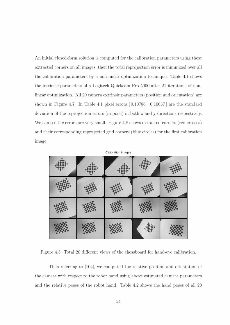
An initial closed-form solution is computed for the calibration parameters using these

extracted corners on all images, then the total reprojection error is minimized over all

the calibration parameters by a non-linear optimization technique. Table 4.1 shows

the intrinsic parameters of a Logitech Quickcam Pro 5000 after 21 iterations of non-

linear optimization. All 20 camera extrinsic parameters (position and orientation) are

shown in Figure 4.7. In Table 4.1 pixel errors [ 0.10786 0.10637 ] are the standard

deviation of the reprojection errors (in pixel) in both x and y directions respectively.

We can see the errors are very small. Figure 4.8 shows extracted corners (red crosses)

and their corresponding reprojected grid corners (blue circles) for the first calibration

image.

Calibration images

Figure 4.5: Total 20 different views of the chessboard for hand-eye calibration.

Then referring to [104], we computed the relative position and orientation of

the camera with respect to the robot hand using above estimated camera parameters

and the relative poses of the robot hand. Table 4.2 shows the hand poses of all 20

54

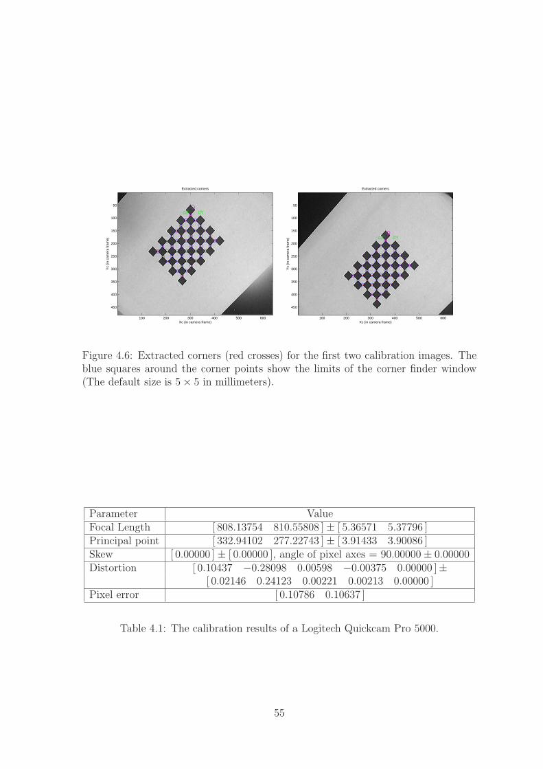
OdX dY

Xc (in camera frame)

Yc

(in c

amer

a fr

ame)

Extracted corners

100 200 300 400 500 600

50

100

150

200

250

300

350

400

450

OdX dY

Xc (in camera frame)

Yc

(in c

amer

a fr

ame)

Extracted corners

100 200 300 400 500 600

50

100

150

200

250

300

350

400

450

Figure 4.6: Extracted corners (red crosses) for the first two calibration images. Theblue squares around the corner points show the limits of the corner finder window(The default size is 5× 5 in millimeters).

Parameter ValueFocal Length [ 808.13754 810.55808 ]± [ 5.36571 5.37796 ]Principal point [ 332.94102 277.22743 ]± [ 3.91433 3.90086 ]Skew [ 0.00000 ]± [ 0.00000 ], angle of pixel axes = 90.00000± 0.00000Distortion [ 0.10437 −0.28098 0.00598 −0.00375 0.00000 ]±

[ 0.02146 0.24123 0.00221 0.00213 0.00000 ]Pixel error [ 0.10786 0.10637 ]

Table 4.1: The calibration results of a Logitech Quickcam Pro 5000.

55

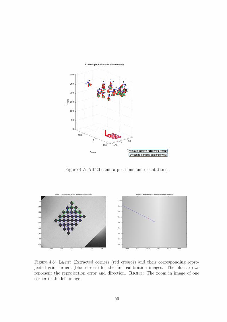
−100

0

100 −500

50

0

50

100

150

200

250

300

Yworld

18

7

5

6178

1615

20

14

9

14

Extrinsic parameters (world−centered)

32

10

131211

Xworld

19

Zw

orld

Figure 4.7: All 20 camera positions and orientations.

XY

O

Image 1 − Image points (+) and reprojected grid points (o)

100 200 300 400 500 600

50

100

150

200

250

300

350

400

450

Image 1 − Image points (+) and reprojected grid points (o)

283.4 283.6 283.8 284 284.2 284.4

230

230.1

230.2

230.3

230.4

230.5

230.6

230.7

230.8

Figure 4.8: Left: Extracted corners (red crosses) and their corresponding repro-jected grid corners (blue circles) for the first calibration images. The blue arrowsrepresent the reprojection error and direction. Right: The zoom in image of onecorner in the left image.

56

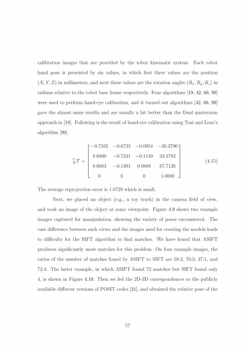
calibration images that are provided by the robot kinematic system. Each robot

hand pose is presented by six values, in which first three values are the position

(X, Y, Z) in millimeters, and next three values are the rotation angles (Rx, Ry, Rz) in

radians relative to the robot base frame respectively. Four algorithms [19, 42, 66, 99]

were used to perform hand-eye calibration, and it turned out algorithms [42, 66, 99]

gave the almost same results and are usually a bit better than the Dual quaternion

approach in [19]. Following is the result of hand-eye calibration using Tsai and Lenz’s

algorithm [99].

CHT =

−0.7332 −0.6733 −0.0954 −20.3796

0.6800 −0.7241 −0.1149 33.2782

0.0083 −0.1491 0.9888 67.7126

0 0 0 1.0000

(4.15)

The average reprojection error is 1.0729 which is small.

Next, we placed an object (e.g., a toy truck) in the camera field of view,

and took an image of the object at some viewpoint. Figure 4.9 shows two example

images captured for manipulation, showing the variety of poses encountered. The

vast difference between such views and the images used for creating the models leads

to difficulty for the SIFT algorithm to find matches. We have found that ASIFT

produces significantly more matches for this problem. On four example images, the

ratios of the number of matches found by ASIFT to SIFT are 58:2, 70:3, 37:1, and

72:4. The latter example, in which ASIFT found 72 matches but SIFT found only

4, is shown in Figure 4.10. Then we fed the 2D-3D correspondences to the publicly

available different versions of POSIT codes [21], and obtained the relative pose of the

57

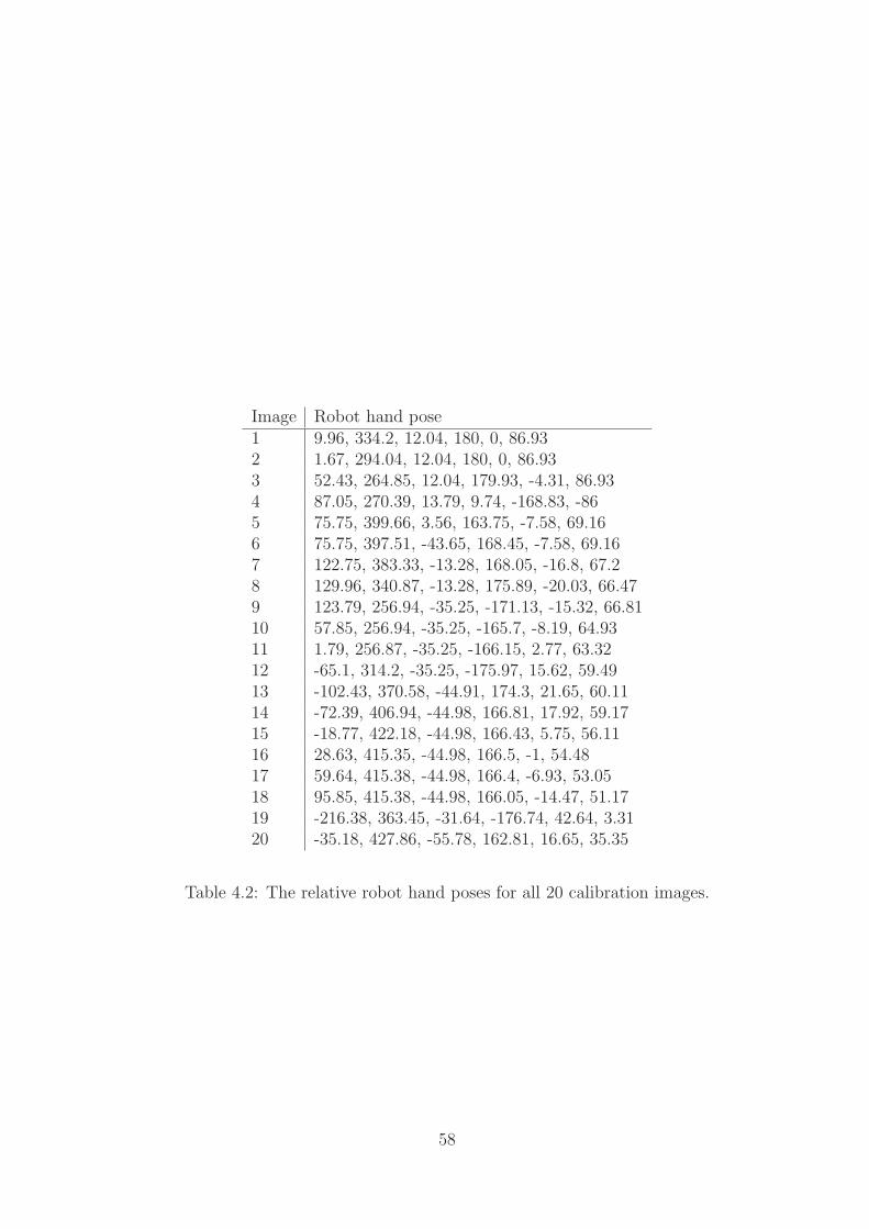
Image Robot hand pose1 9.96, 334.2, 12.04, 180, 0, 86.932 1.67, 294.04, 12.04, 180, 0, 86.933 52.43, 264.85, 12.04, 179.93, -4.31, 86.934 87.05, 270.39, 13.79, 9.74, -168.83, -865 75.75, 399.66, 3.56, 163.75, -7.58, 69.166 75.75, 397.51, -43.65, 168.45, -7.58, 69.167 122.75, 383.33, -13.28, 168.05, -16.8, 67.28 129.96, 340.87, -13.28, 175.89, -20.03, 66.479 123.79, 256.94, -35.25, -171.13, -15.32, 66.8110 57.85, 256.94, -35.25, -165.7, -8.19, 64.9311 1.79, 256.87, -35.25, -166.15, 2.77, 63.3212 -65.1, 314.2, -35.25, -175.97, 15.62, 59.4913 -102.43, 370.58, -44.91, 174.3, 21.65, 60.1114 -72.39, 406.94, -44.98, 166.81, 17.92, 59.1715 -18.77, 422.18, -44.98, 166.43, 5.75, 56.1116 28.63, 415.35, -44.98, 166.5, -1, 54.4817 59.64, 415.38, -44.98, 166.4, -6.93, 53.0518 95.85, 415.38, -44.98, 166.05, -14.47, 51.1719 -216.38, 363.45, -31.64, -176.74, 42.64, 3.3120 -35.18, 427.86, -55.78, 162.81, 16.65, 35.35

Table 4.2: The relative robot hand poses for all 20 calibration images.

58

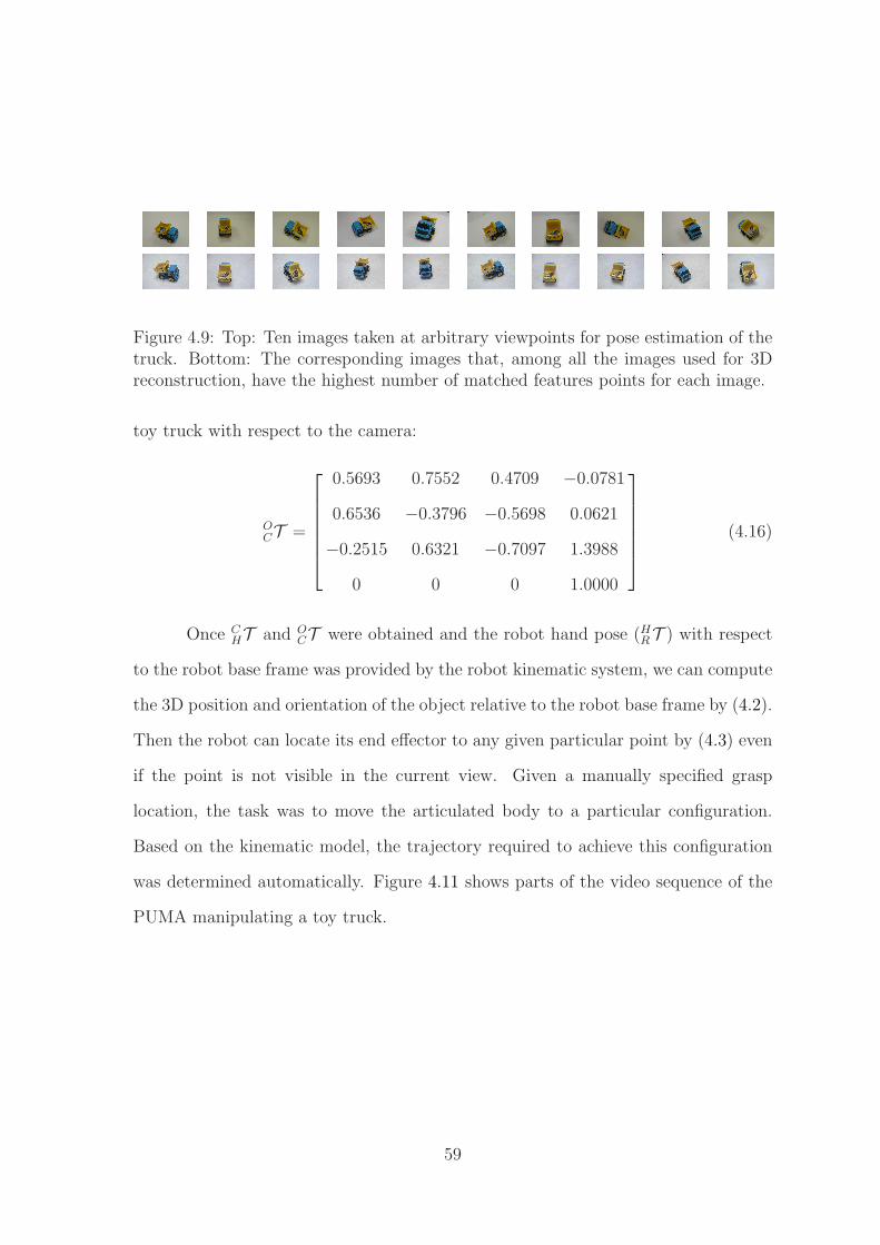
Figure 4.9: Top: Ten images taken at arbitrary viewpoints for pose estimation of thetruck. Bottom: The corresponding images that, among all the images used for 3Dreconstruction, have the highest number of matched features points for each image.

toy truck with respect to the camera:

OCT =

0.5693 0.7552 0.4709 −0.0781

0.6536 −0.3796 −0.5698 0.0621

−0.2515 0.6321 −0.7097 1.3988

0 0 0 1.0000

(4.16)

Once CHT and O

CT were obtained and the robot hand pose (HRT ) with respect

to the robot base frame was provided by the robot kinematic system, we can compute

the 3D position and orientation of the object relative to the robot base frame by (4.2).

Then the robot can locate its end effector to any given particular point by (4.3) even

if the point is not visible in the current view. Given a manually specified grasp

location, the task was to move the articulated body to a particular configuration.

Based on the kinematic model, the trajectory required to achieve this configuration

was determined automatically. Figure 4.11 shows parts of the video sequence of the

PUMA manipulating a toy truck.

59

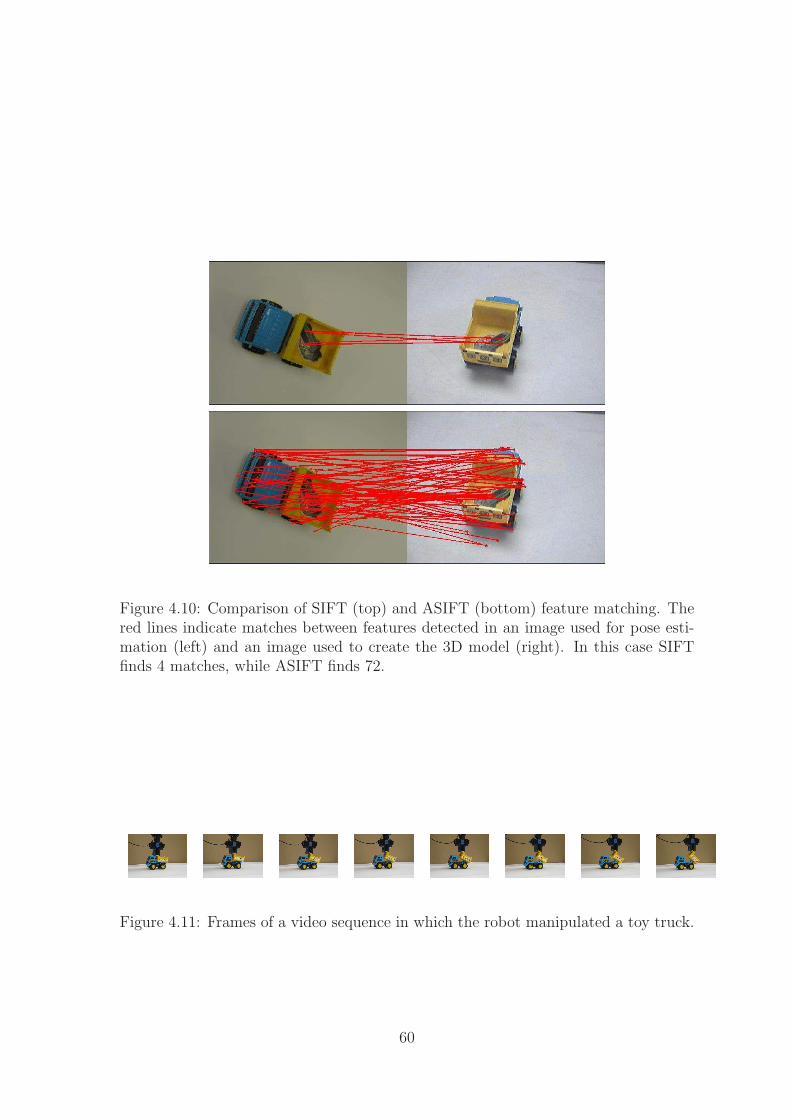
Figure 4.10: Comparison of SIFT (top) and ASIFT (bottom) feature matching. Thered lines indicate matches between features detected in an image used for pose esti-mation (left) and an image used to create the 3D model (right). In this case SIFTfinds 4 matches, while ASIFT finds 72.

Figure 4.11: Frames of a video sequence in which the robot manipulated a toy truck.

60

Chapter 5

Using RGBD Sensors

There is plenty of room for further improvements to the approach presented.

For real-world applications, it will be important to remove the need for artificial

markers attached to objects, whose sole purpose is to facilitate correspondence be-

tween images. One solution to address this issue is to use RGBD sensors that yield

a depth value for each pixel immediately by the sensor itself rather than requiring

correspondence to establish depth. The proposed approach is able to be adapted to

such sensors with only minimal changes in the processing pipeline, leading to much

denser 3D models, as well as reducing the computation time required.

5.1 RGBD sensors

Before we introduce RGBD sensors, we first present the image formation pro-

cess and the range imaging both of which are key parts of RGBD sensors.

61

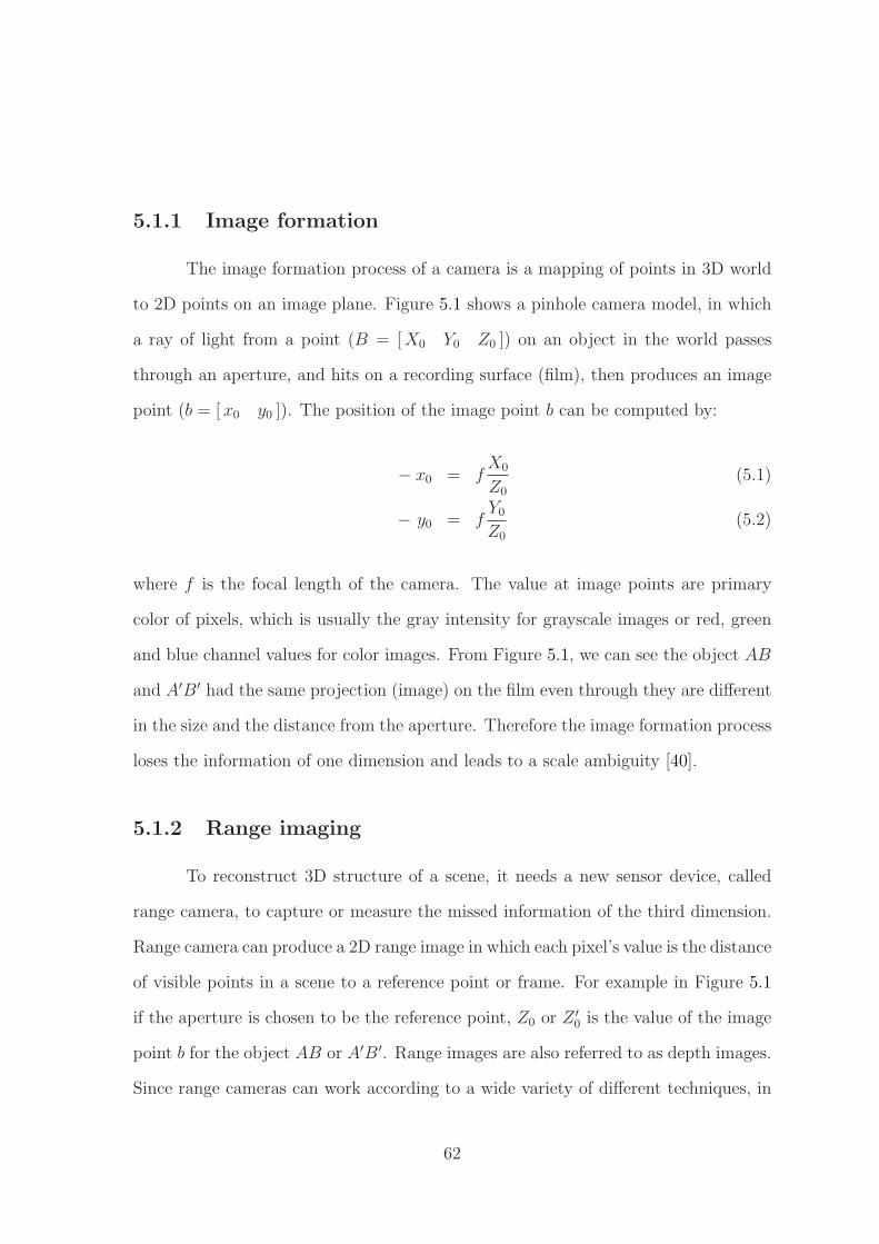
5.1.1 Image formation

The image formation process of a camera is a mapping of points in 3D world

to 2D points on an image plane. Figure 5.1 shows a pinhole camera model, in which

a ray of light from a point (B = [X0 Y0 Z0 ]) on an object in the world passes

through an aperture, and hits on a recording surface (film), then produces an image

point (b = [ x0 y0 ]). The position of the image point b can be computed by:

− x0 = fX0

Z0

(5.1)

− y0 = fY0

Z0

(5.2)

where f is the focal length of the camera. The value at image points are primary

color of pixels, which is usually the gray intensity for grayscale images or red, green

and blue channel values for color images. From Figure 5.1, we can see the object AB

and A′B′ had the same projection (image) on the film even through they are different

in the size and the distance from the aperture. Therefore the image formation process

loses the information of one dimension and leads to a scale ambiguity [40].

5.1.2 Range imaging

To reconstruct 3D structure of a scene, it needs a new sensor device, called

range camera, to capture or measure the missed information of the third dimension.

Range camera can produce a 2D range image in which each pixel’s value is the distance

of visible points in a scene to a reference point or frame. For example in Figure 5.1

if the aperture is chosen to be the reference point, Z0 or Z ′

0 is the value of the image

point b for the object AB or A′B′. Range images are also referred to as depth images.

Since range cameras can work according to a wide variety of different techniques, in

62

Figure 5.1: Pinhole camera model: a ray of light from a point on an object in the worldpasses through an aperture, and hits on a recording surface (film), then produces animage point.

the following sections we only introduce the most common approaches.

5.1.2.1 Stereo triangulation

A stereo camera system consists of a pair of cameras mounted side by side to

obtain left and right images, simulating human binocular vision. Figure 5.2 shows

the standard stereo model for two pinhole cameras whose optical axes are parallel. C

and C ′ are lens centers of cameras, and the left and right image planes are coplanar.

In the model, a world point Q is projected into a pair of corresponding points q and

q′ on the left and right image, and lies at the intersection of two rays from q through

C and from q′ through C ′ respectively.

The stereo triangulation is to find the intersection of the two rays in 3D space.

From Figure 5.2, it’s easy to find two triangles (Qqq′) and (QCC ′) are similar, there-

fore we get

b+ x− x′

b=

f + Z

Z. (5.3)

63

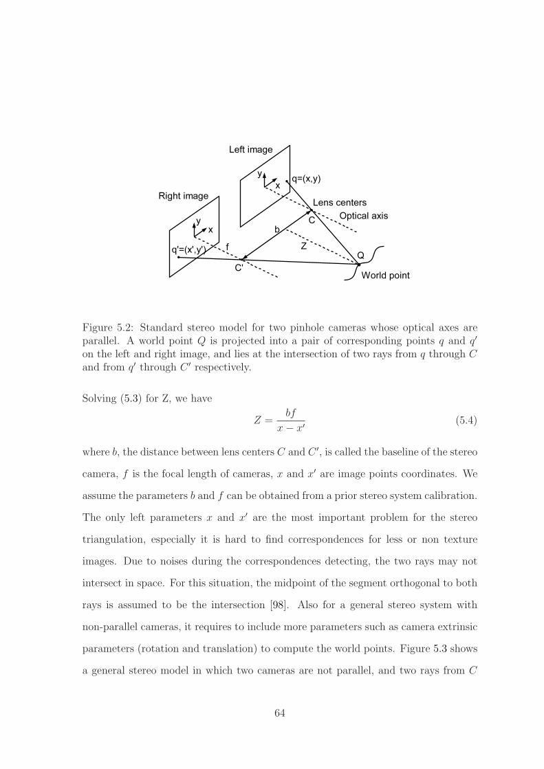
Figure 5.2: Standard stereo model for two pinhole cameras whose optical axes areparallel. A world point Q is projected into a pair of corresponding points q and q′

on the left and right image, and lies at the intersection of two rays from q through Cand from q′ through C ′ respectively.

Solving (5.3) for Z, we have

Z =bf

x− x′(5.4)

where b, the distance between lens centers C and C ′, is called the baseline of the stereo

camera, f is the focal length of cameras, x and x′ are image points coordinates. We

assume the parameters b and f can be obtained from a prior stereo system calibration.

The only left parameters x and x′ are the most important problem for the stereo

triangulation, especially it is hard to find correspondences for less or non texture

images. Due to noises during the correspondences detecting, the two rays may not

intersect in space. For this situation, the midpoint of the segment orthogonal to both

rays is assumed to be the intersection [98]. Also for a general stereo system with

non-parallel cameras, it requires to include more parameters such as camera extrinsic

parameters (rotation and translation) to compute the world points. Figure 5.3 shows

a general stereo model in which two cameras are not parallel, and two rays from C

64

Figure 5.3: General stereo model for two non-parallel cameras. Two rays from Cthrough q and from C ′ through q′ do not intersect due to some noises. The midpointQ of the segment ab that is orthogonal to both rays is assumed to be the world point.

through q and from C ′ through q′ do not intersect due to some errors. Therefore the

midpoint Q of the segment ab that is orthogonal to both rays is assumed to be the

world point.

5.1.2.2 Structured lighting

Structured lighting is an approach to extract geometric structure of objects in

a scene by projecting known light patterns onto the scene. The approach effectively

solves correspondences problem by searching the patterns in the camera image instead

of using classic feature matching techniques. Common used light patterns are rays,

planes, grids, parallel stripes, encoded lights and so on. A standard structured light

3D scanner consists of one light source and one camera. Figure 5.4 shows a simple

model in 2D , in which a laser light source projects a light spot on an object surface

and a camera observes the spot. For the triangle (OPL), according to law of sines,

65

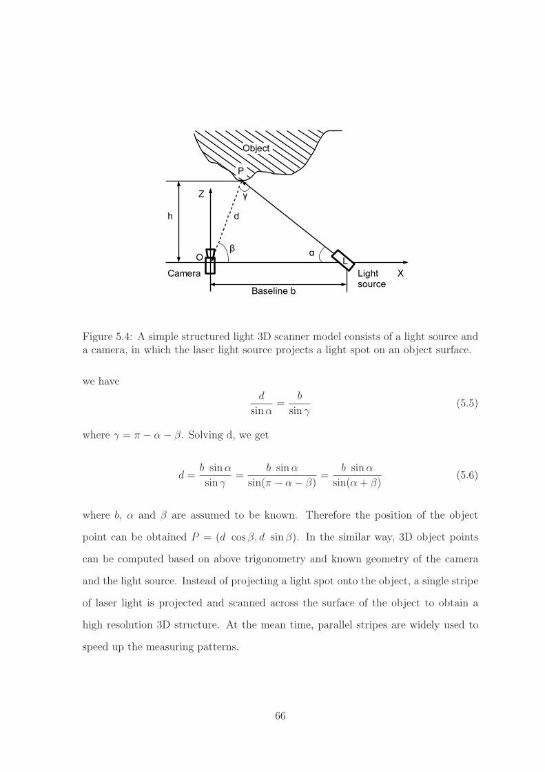
Figure 5.4: A simple structured light 3D scanner model consists of a light source anda camera, in which the laser light source projects a light spot on an object surface.

we have

d

sinα=

b

sin γ(5.5)

where γ = π − α− β. Solving d, we get

d =b sinα

sin γ=

b sinα

sin(π − α− β)=

b sinα

sin(α + β)(5.6)

where b, α and β are assumed to be known. Therefore the position of the object

point can be obtained P = (d cos β, d sin β). In the similar way, 3D object points

can be computed based on above trigonometry and known geometry of the camera

and the light source. Instead of projecting a light spot onto the object, a single stripe

of laser light is projected and scanned across the surface of the object to obtain a

high resolution 3D structure. At the mean time, parallel stripes are widely used to

speed up the measuring patterns.

66

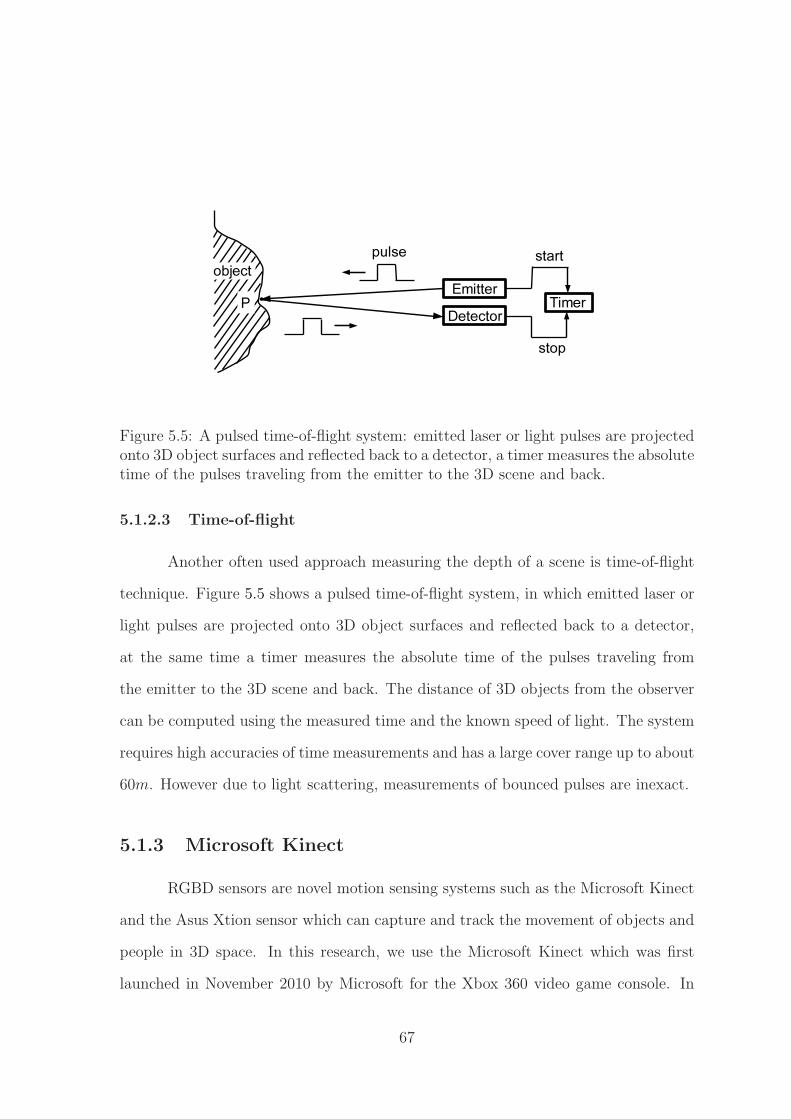
Figure 5.5: A pulsed time-of-flight system: emitted laser or light pulses are projectedonto 3D object surfaces and reflected back to a detector, a timer measures the absolutetime of the pulses traveling from the emitter to the 3D scene and back.

5.1.2.3 Time-of-flight

Another often used approach measuring the depth of a scene is time-of-flight

technique. Figure 5.5 shows a pulsed time-of-flight system, in which emitted laser or

light pulses are projected onto 3D object surfaces and reflected back to a detector,

at the same time a timer measures the absolute time of the pulses traveling from

the emitter to the 3D scene and back. The distance of 3D objects from the observer

can be computed using the measured time and the known speed of light. The system

requires high accuracies of time measurements and has a large cover range up to about

60m. However due to light scattering, measurements of bounced pulses are inexact.

5.1.3 Microsoft Kinect

RGBD sensors are novel motion sensing systems such as the Microsoft Kinect

and the Asus Xtion sensor which can capture and track the movement of objects and

people in 3D space. In this research, we use the Microsoft Kinect which was first

launched in November 2010 by Microsoft for the Xbox 360 video game console. In

67

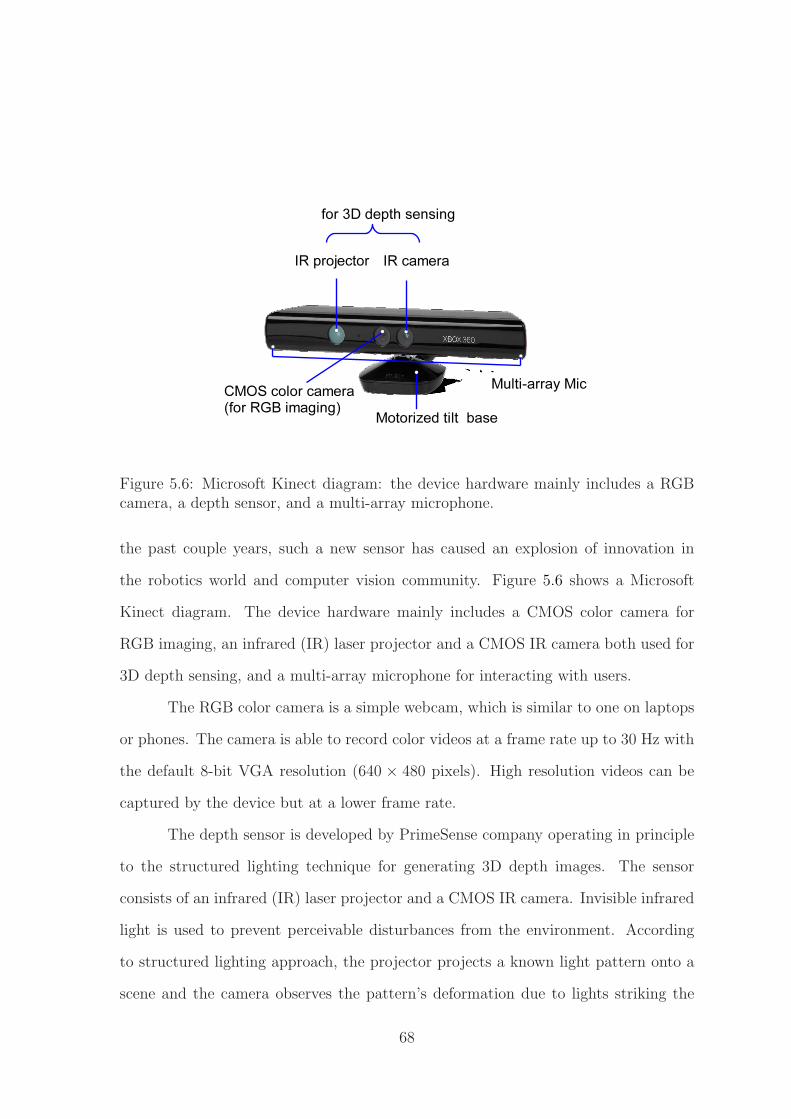
Figure 5.6: Microsoft Kinect diagram: the device hardware mainly includes a RGBcamera, a depth sensor, and a multi-array microphone.

the past couple years, such a new sensor has caused an explosion of innovation in

the robotics world and computer vision community. Figure 5.6 shows a Microsoft

Kinect diagram. The device hardware mainly includes a CMOS color camera for

RGB imaging, an infrared (IR) laser projector and a CMOS IR camera both used for

3D depth sensing, and a multi-array microphone for interacting with users.

The RGB color camera is a simple webcam, which is similar to one on laptops

or phones. The camera is able to record color videos at a frame rate up to 30 Hz with

the default 8-bit VGA resolution (640 × 480 pixels). High resolution videos can be

captured by the device but at a lower frame rate.

The depth sensor is developed by PrimeSense company operating in principle

to the structured lighting technique for generating 3D depth images. The sensor

consists of an infrared (IR) laser projector and a CMOS IR camera. Invisible infrared

light is used to prevent perceivable disturbances from the environment. According

to structured lighting approach, the projector projects a known light pattern onto a

scene and the camera observes the pattern’s deformation due to lights striking the

68

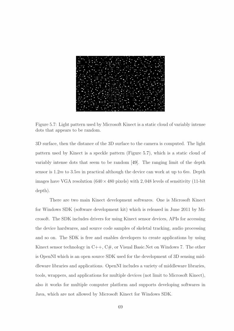
Figure 5.7: Light pattern used by Microsoft Kinect is a static cloud of variably intensedots that appears to be random.

3D surface, then the distance of the 3D surface to the camera is computed. The light

pattern used by Kinect is a speckle pattern (Figure 5.7), which is a static cloud of

variably intense dots that seem to be random [49]. The ranging limit of the depth

sensor is 1.2m to 3.5m in practical although the device can work at up to 6m. Depth

images have VGA resolution (640×480 pixels) with 2, 048 levels of sensitivity (11-bit

depth).

There are two main Kinect development softwares. One is Microsoft Kinect

for Windows SDK (software development kit) which is released in June 2011 by Mi-

crosoft. The SDK includes drivers for using Kinect sensor devices, APIs for accessing

the device hardwares, and source code samples of skeletal tracking, audio processing

and so on. The SDK is free and enables developers to create applications by using

Kinect sensor technology in C++, C#, or Visual Basic.Net on Windows 7. The other

is OpenNI which is an open source SDK used for the development of 3D sensing mid-

dleware libraries and applications. OpenNI includes a variety of middleware libraries,

tools, wrappers, and applications for multiple devices (not limit to Microsoft Kinect),

also it works for multiple computer platform and supports developing softwares in

Java, which are not allowed by Microsoft Kinect for Windows SDK.

69

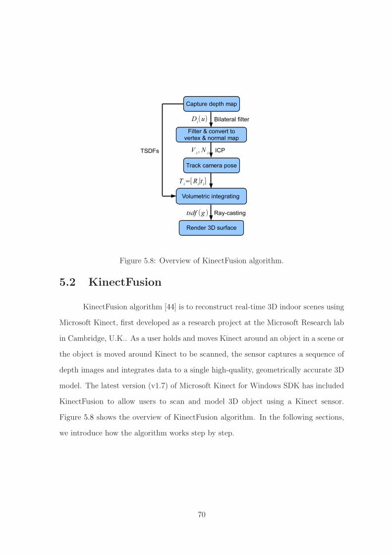
Figure 5.8: Overview of KinectFusion algorithm.

5.2 KinectFusion

KinectFusion algorithm [44] is to reconstruct real-time 3D indoor scenes using

Microsoft Kinect, first developed as a research project at the Microsoft Research lab

in Cambridge, U.K.. As a user holds and moves Kinect around an object in a scene or

the object is moved around Kinect to be scanned, the sensor captures a sequence of

depth images and integrates data to a single high-quality, geometrically accurate 3D

model. The latest version (v1.7) of Microsoft Kinect for Windows SDK has included

KinectFusion to allow users to scan and model 3D object using a Kinect sensor.

Figure 5.8 shows the overview of KinectFusion algorithm. In the following sections,

we introduce how the algorithm works step by step.

70

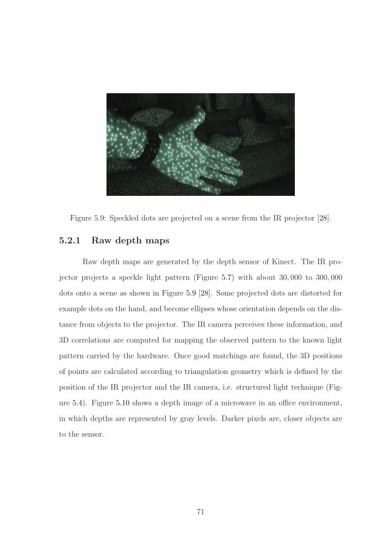
Figure 5.9: Speckled dots are projected on a scene from the IR projector [28].

5.2.1 Raw depth maps

Raw depth maps are generated by the depth sensor of Kinect. The IR pro-

jector projects a speckle light pattern (Figure 5.7) with about 30, 000 to 300, 000

dots onto a scene as shown in Figure 5.9 [28]. Some projected dots are distorted for

example dots on the hand, and become ellipses whose orientation depends on the dis-

tance from objects to the projector. The IR camera perceives these information, and

3D correlations are computed for mapping the observed pattern to the known light

pattern carried by the hardware. Once good matchings are found, the 3D positions

of points are calculated according to triangulation geometry which is defined by the

position of the IR projector and the IR camera, i.e. structured light technique (Fig-

ure 5.4). Figure 5.10 shows a depth image of a microwave in an office environment,

in which depths are represented by gray levels. Darker pixels are, closer objects are

to the sensor.

71

Figure 5.10: Depth image of a microwave in an office environment. Depths arerepresented by gray levels.

5.2.2 Vertex and normal maps

In raw depth maps, there are many pixels without depth values due to noises.

To remove erroneous measurements, KinectFusion algorithm applies a bilateral filter

to raw depth maps. This is just for converting depth maps to vertex and normal

maps. Raw depth data are still be used for recovering the 3D structure. A vertex

map is a 3D point cloud about visible objects in a scene with respect to the camera

coordinate system, in which the origin locates at the principal point and the z-axis

points to the scene. For each point (x, y) with a depth value (d) in a depth map, the

corresponding 3D vertex v(x, y) in metric units is obtained by

v(x, y) =

X

Y

Z

= d K−1

x

y

1

(5.7)

72

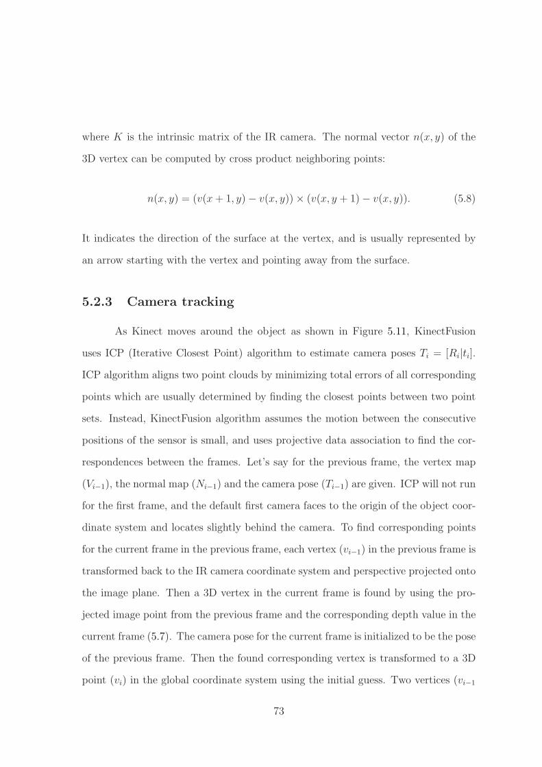
where K is the intrinsic matrix of the IR camera. The normal vector n(x, y) of the

3D vertex can be computed by cross product neighboring points:

n(x, y) = (v(x+ 1, y)− v(x, y))× (v(x, y + 1)− v(x, y)). (5.8)

It indicates the direction of the surface at the vertex, and is usually represented by

an arrow starting with the vertex and pointing away from the surface.

5.2.3 Camera tracking

As Kinect moves around the object as shown in Figure 5.11, KinectFusion

uses ICP (Iterative Closest Point) algorithm to estimate camera poses Ti = [Ri|ti].

ICP algorithm aligns two point clouds by minimizing total errors of all corresponding

points which are usually determined by finding the closest points between two point

sets. Instead, KinectFusion algorithm assumes the motion between the consecutive

positions of the sensor is small, and uses projective data association to find the cor-

respondences between the frames. Let’s say for the previous frame, the vertex map

(Vi−1), the normal map (Ni−1) and the camera pose (Ti−1) are given. ICP will not run

for the first frame, and the default first camera faces to the origin of the object coor-

dinate system and locates slightly behind the camera. To find corresponding points

for the current frame in the previous frame, each vertex (vi−1) in the previous frame is

transformed back to the IR camera coordinate system and perspective projected onto

the image plane. Then a 3D vertex in the current frame is found by using the pro-

jected image point from the previous frame and the corresponding depth value in the

current frame (5.7). The camera pose for the current frame is initialized to be the pose

of the previous frame. Then the found corresponding vertex is transformed to a 3D

point (vi) in the global coordinate system using the initial guess. Two vertices (vi−1

73

Figure 5.11: Camera tracking in KinectFusion.

and vi) which either are too far or whose normal difference is too large are assumed

to be outliers and rejected by the system. Otherwise two vertices are determined

as the correspondences. Then a new transformation is computed using these set of

correspondences. Above process is repeated until finding a final transformation (Ti)

which minimizes the point-to-plane error between two surfaces. Also KinectFusion

algorithm generates a vertex and normal map pyramid to improve camera tracking

performance. The pyramid is normally 3 levels, and it down samples the depth map

twice.

5.2.4 Volumetric integrating

To integrate the current raw depth data into the 3D model, KinectFusion

algorithm uses a volumetric representation and Truncated Signed Distance Functions

(TSDFs). A default 3D volume is a 3× 3× 3 cube in meters as shown in Figure 5.11,

which is subdivided uniformly into a set of voxels for example 512 voxels per axis. The

74

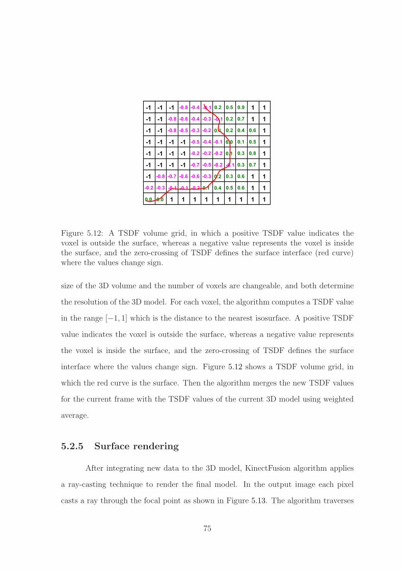
Figure 5.12: A TSDF volume grid, in which a positive TSDF value indicates thevoxel is outside the surface, whereas a negative value represents the voxel is insidethe surface, and the zero-crossing of TSDF defines the surface interface (red curve)where the values change sign.

size of the 3D volume and the number of voxels are changeable, and both determine

the resolution of the 3D model. For each voxel, the algorithm computes a TSDF value

in the range [−1, 1] which is the distance to the nearest isosurface. A positive TSDF

value indicates the voxel is outside the surface, whereas a negative value represents

the voxel is inside the surface, and the zero-crossing of TSDF defines the surface

interface where the values change sign. Figure 5.12 shows a TSDF volume grid, in

which the red curve is the surface. Then the algorithm merges the new TSDF values

for the current frame with the TSDF values of the current 3D model using weighted

average.

5.2.5 Surface rendering

After integrating new data to the 3D model, KinectFusion algorithm applies

a ray-casting technique to render the final model. In the output image each pixel

casts a ray through the focal point as shown in Figure 5.13. The algorithm traverses

75

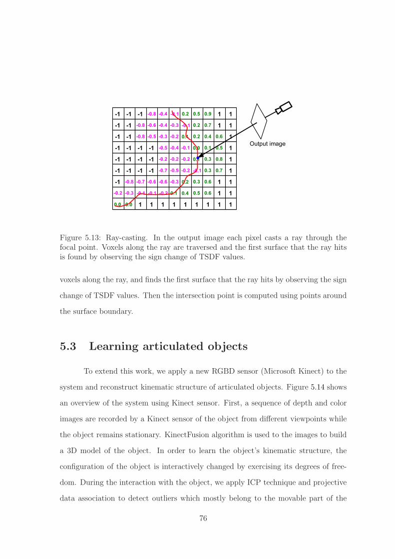
Figure 5.13: Ray-casting. In the output image each pixel casts a ray through thefocal point. Voxels along the ray are traversed and the first surface that the ray hitsis found by observing the sign change of TSDF values.

voxels along the ray, and finds the first surface that the ray hits by observing the sign

change of TSDF values. Then the intersection point is computed using points around

the surface boundary.

5.3 Learning articulated objects

To extend this work, we apply a new RGBD sensor (Microsoft Kinect) to the

system and reconstruct kinematic structure of articulated objects. Figure 5.14 shows

an overview of the system using Kinect sensor. First, a sequence of depth and color

images are recorded by a Kinect sensor of the object from different viewpoints while

the object remains stationary. KinectFusion algorithm is used to the images to build

a 3D model of the object. In order to learn the object’s kinematic structure, the

configuration of the object is interactively changed by exercising its degrees of free-

dom. During the interaction with the object, we apply ICP technique and projective

data association to detect outliers which mostly belong to the movable part of the

76

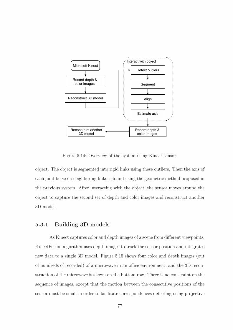
Figure 5.14: Overview of the system using Kinect sensor.

object. The object is segmented into rigid links using these outliers. Then the axis of

each joint between neighboring links is found using the geometric method proposed in

the previous system. After interacting with the object, the sensor moves around the

object to capture the second set of depth and color images and reconstruct another

3D model.

5.3.1 Building 3D models

As Kinect captures color and depth images of a scene from different viewpoints,

KinectFusion algorithm uses depth images to track the sensor position and integrates

new data to a single 3D model. Figure 5.15 shows four color and depth images (out

of hundreds of recorded) of a microwave in an office environment, and the 3D recon-

struction of the microwave is shown on the bottom row. There is no constraint on the

sequence of images, except that the motion between the consecutive positions of the

sensor must be small in order to facilitate correspondences detecting using projective

77

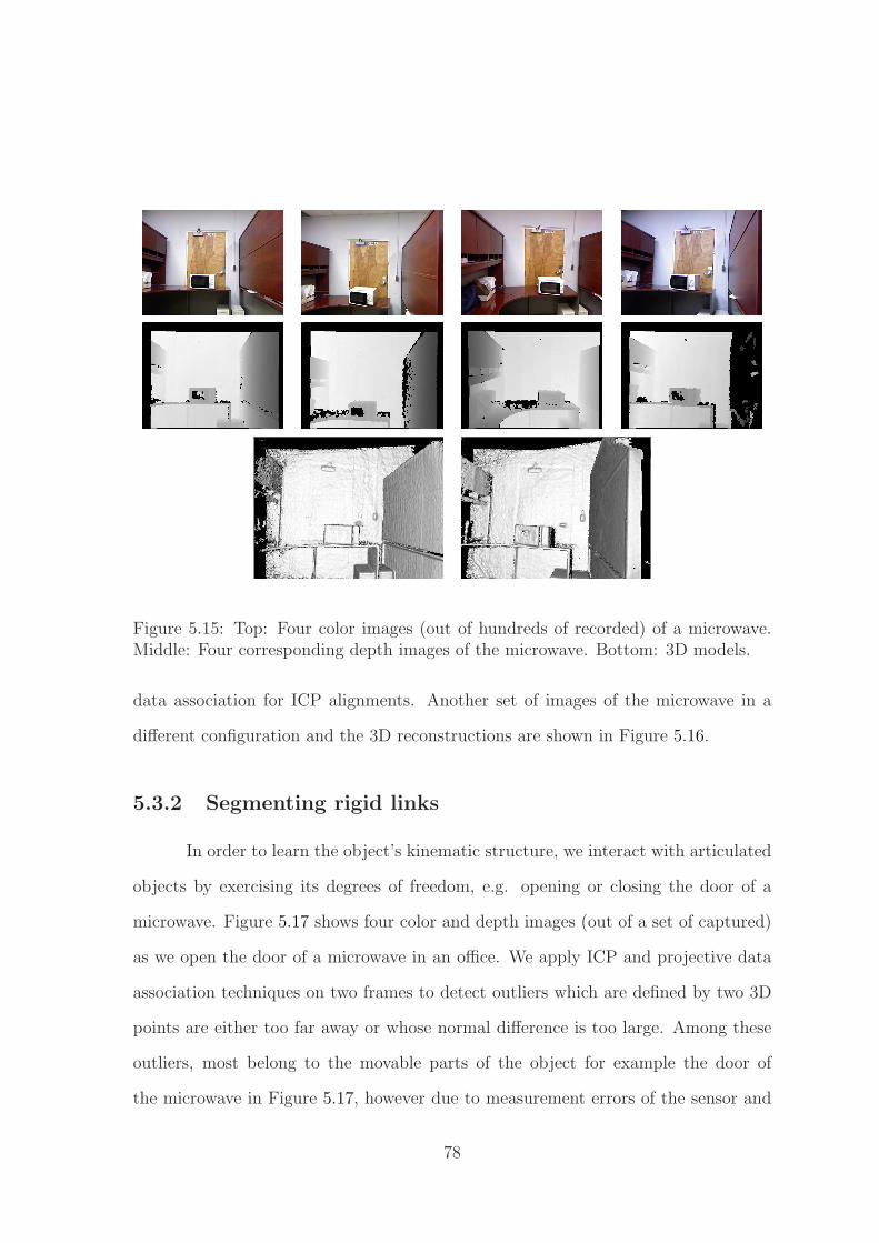
Figure 5.15: Top: Four color images (out of hundreds of recorded) of a microwave.Middle: Four corresponding depth images of the microwave. Bottom: 3D models.

data association for ICP alignments. Another set of images of the microwave in a

different configuration and the 3D reconstructions are shown in Figure 5.16.

5.3.2 Segmenting rigid links

In order to learn the object’s kinematic structure, we interact with articulated

objects by exercising its degrees of freedom, e.g. opening or closing the door of a

microwave. Figure 5.17 shows four color and depth images (out of a set of captured)

as we open the door of a microwave in an office. We apply ICP and projective data

association techniques on two frames to detect outliers which are defined by two 3D

points are either too far away or whose normal difference is too large. Among these

outliers, most belong to the movable parts of the object for example the door of

the microwave in Figure 5.17, however due to measurement errors of the sensor and

78

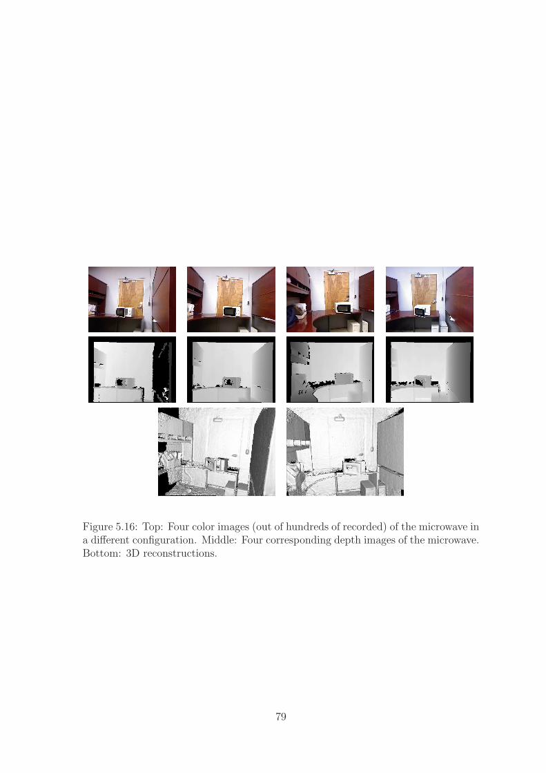
Figure 5.16: Top: Four color images (out of hundreds of recorded) of the microwave ina different configuration. Middle: Four corresponding depth images of the microwave.Bottom: 3D reconstructions.

79

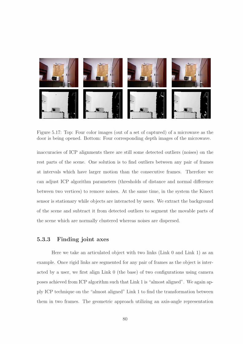
Figure 5.17: Top: Four color images (out of a set of captured) of a microwave as thedoor is being opened. Bottom: Four corresponding depth images of the microwave.

inaccuracies of ICP alignments there are still some detected outliers (noises) on the

rest parts of the scene. One solution is to find outliers between any pair of frames

at intervals which have larger motion than the consecutive frames. Therefore we

can adjust ICP algorithm parameters (thresholds of distance and normal difference

between two vertices) to remove noises. At the same time, in the system the Kinect

sensor is stationary while objects are interacted by users. We extract the background

of the scene and subtract it from detected outliers to segment the movable parts of

the scene which are normally clustered whereas noises are dispersed.

5.3.3 Finding joint axes

Here we take an articulated object with two links (Link 0 and Link 1) as an

example. Once rigid links are segmented for any pair of frames as the object is inter-

acted by a user, we first align Link 0 (the base) of two configurations using camera

poses achieved from ICP algorithm such that Link 1 is “almost aligned”. We again ap-

ply ICP technique on the “almost aligned” Link 1 to find the transformation between

them in two frames. The geometric approach utilizing an axis-angle representation

80

proposed in the previous system is then used to estimate the axis of the joint.

Figure 5.18 shows the estimated rotation axis (the red line) of a microwave

in an office for two frames. The extended approach using a RGBD sensor is able

to reconstruct much denser 3D models, segment the points into the individual links,

and estimate the axis of rotation. Also it does not require artificial markers attached

to the objects and is able to handle the less textured or untextured objects. The

resulting models therefore include dense 3D point clouds representing the surfaces

of the objects, along with the joint parameters. Another advantage of the approach

is it does not require more than two configurations of the objects, therefore we can

obtain one joint axis for any two frames with object motions and average these axes

parameters (direction and location) to yield a final estimation.

One limitation of the above proposed approach is the assumption of Kinect-

Fusion algorithm, that is the motion between two consecutive sensor positions is

small. With this assumption, KinectFusion detects the correspondences between the

consecutive frames using projective data association technique instead of using the

classic feature detectors, and further tracks camera poses by applying ICP algorithm.

Since we use the detected correspondences and estimated camera poses to compute

the transformation of rigid links between the frames and segment rigid links, the

accuracy of detected correspondences affects the performance of the approach. For

the case of a large sensor motion, we can apply the classic features detectors such

as ASIFT feature detector or line detector to filter the mismatched correspondences

found by KinectFusion.

81

Figure 5.18: Red lines are the estimated rotation axes of a microwave for two differentframes while the object is interacted by users.

82

Chapter 6

Conclusion

Autonomous operation in unstructured and dynamic environments has become

an important trend in robotics. As robots move into unstructured environments such

as homes, schools, and workplaces, new approaches to sensing and manipulation are

required to handle the greater variety of objects encountered. For example, rather

than expecting the robot to have advanced knowledge of all objects that will be

encountered in the physical world, the ability to actively learn about the scene will

be crucial. Recently reconstructing articulated objects has caught the attention of

researchers. These objects consist of rigid links connected by one or more revolute or

prismatic joints. A number of everyday objects, such as laptop computers, staplers,

scissors, cabinet drawers, doors, and some cell phones fit such a model. Even a desk

or chair sliding on the floor can be modeled, to some degree, as a set of prismatic and

revolute joints.

83

6.1 Contributions

This work has presented novel algorithms regarding articulated objects re-

construction and operation. The main contributions of this dissertation are listed

below.

1. An algorithm called Procrustes-Lo-RANSAC (PLR) is proposed to extract the

3D surface and kinematic structure of articulated objects. Multiple pictures are

taken of an object by a single uncalibrated camera in two different configura-

tions, and 3D models are reconstructed using structure-from-motion techniques.

From these models, the rigid links of the object are segmented and aligned, al-

lowing the joint axes to be estimated using a geometric approach. From the

performance aspect, the algorithm

• recovers occlusion-aware multi-view models which refer to a system that

has knowledge about parts of the object that are not currently visible.

• does not require prior knowledge of the object,

• does not make any assumptions regarding planarity of the object,

• supports both revolute and prismatic joints,

• automatically classifies joints type,

• works for objects with multiple joints,

• only requires two different configurations of the object,

• shows its effectiveness on a range of environmental conditions with various

types of objects useful in domestic robotics.

2. The resulting occlusion-aware 3D articulated model can be used to enable a

robot to manipulate the object. Two capabilities are supported by such a

84

model:

• Given a particular point on the object, the robot can move its end effector

to that position, even if the point is not visible in the current view. This

is one of the main advantages of the occlusion-aware approach, namely,

that the robot is not limited only to the side of the object that is currently

visible, but rather that a full 3D model is available.

• Given a particular grasp point, the robot can grab the object at that point

and move in such a way so as to exercise the articulated joint.

3. A RGBD sensor (Microsoft Kinect) is used to improve the proposed approach.

Kinect sensor captures not only a sequence of color images but also depth images

of a scene, which facilitates the correspondences detection and camera tracking.

KinectFusion algorithm is applied to yield a single high-quality, geometrically

accurate 3D model from which rigid links of the object are segmented and

aligned, allowing the joint axes to be estimated using the proposed geometric

approach. From the performance aspect, the algorithm

• does not require artificial markers attached to objects,

• yields much denser 3D models,

• reduces the computation time.

6.2 Future work

There is plenty of room for further improvements in this work. First, the pro-

posed algorithm (PLR) is challenged by less textured or untextured objects. This

limitation can be solved by attaching artificial markers to objects which is very com-

mon in the computer vision community. However for real-world applications it is

85

important to remove this need whose sole purpose is to facilitate correspondence be-

tween images. One possible solution to address this issue is to incorporate additional

features such as line features into the proposed algorithm to increase performance.

Comparing to point features (SIFT, SURF and so on), line features mostly locate at

edges of objects or scenes and encode geometrical and structural information about

them. Apart from including other 2D features, the algorithm could use 3D features

like fast point feature histograms (FPFH) descriptors or viewpoint feature histogram

(VFH) descriptors to find the correspondences between 3D models.

Another improvement would be to use new RGBD sensors instead of regular

cameras as we introduced in Chapter 5. However KinectFusion is limited to work well

when the motion between two consecutive sensor positions is small, which facilitates

correspondences finding between frames during tracking camera poses using ICP and

projective data association techniques. Moreover, this work could be extended to

handle other types of joints presented in articulated objects section such as ball joints.

86

Bibliography

[1] Blender, http://www.blender.org/.

[2] Intel OpenCV library, http://www.intel.com/research/mrl/research/opencv/.

[3] 2009. Computing Community Consortium. A Roadmap for US Robotics: FromInternet to Robotics. http://www.us-robotics.us/reports/CCC%20Report.pdf.

[4] S. Agarwal, N. Snavely, I. Simon, S. M. Seitz, and R. Szeliski. Building Romein a day. In Proceedings of the International Conference on Computer Vision,Sept. 2009.

[5] N. Andreff, R. Horaud, and B. Espiau. Robot hand-eye calibration usingstructure from motion. International Journal of Robotics Research (IJRR),20(3):228–248, Mar. 2001.

[6] G. M. Bone, A. Lambert, and M. Edwards. Automated modeling and roboticgrasping of unknown three-dimensional objects. In Proceedings of the Interna-tional Conference on Robotics and Automation, May 2008.

[7] F. Bonin-Font, A. Ortiz, and G. Oliver. Visual navigation for mobile robots: Asurvey. Journal of Intelligent and Robotic Systems, 53(3):263–296, Nov. 2008.

[8] J.-Y. Bouguet, 2010. Complete Camera Calibration Toolbox for Matlab,http://www.vision.caltech.edu/bouguetj/calib doc/index.html.

[9] C. Bregler, A. Hertzmann, and H. Biermann. Recovering non-rigid 3D shapefrom image streams. In Proceedings of the IEEE Conference on Computer Vi-sion and Pattern Recognition (CVPR), 2000.

[10] A. Broadhurst, T. W. Drummond, and R. Cipolla. A probabilistic frameworkfor space carving. In Proceedings of the International Conference on ComputerVision, pages 388–393, July 2001.

[11] M. Brown and D. G. Lowe. Unsupervised 3D object recognition and reconstruc-tion in unordered datasets. In Proceedings of the International Conference on3D Digital Imaging and Modelling, pages 56–63, 2005.

87

[12] A. O. Balan, L. Sigal, M. J. Black, J. E. Davis, and H. W. Haussecker. Detailedhuman shape and pose from images. In Proceedings of the IEEE Conference onComputer Vision and Pattern Recognition (CVPR), 2007.

[13] M. D. Choi. Notes on the norm estimates for the sum of two matrices. ActaMathematica Sinica, 19(3):595–598, July 2003.

[14] O. Chum, J. Matas, and J. Kittler. Locally optimized RANSAC. Proceedingsof the 25th DAGM Symposium, pages 236–243, Sept. 2003.

[15] R. Collins. A space-sweep approach to true multi-image matching. In Pro-ceedings of the IEEE Conference on Computer Vision and Pattern Recognition(CVPR), pages 358–363, June 1996.

[16] J. Costeira and T. Kanade. A multi-body factorization method for motionanalysis. In Proceedings of the International Conference on Computer Vision,pages 1071–1076, 1995.

[17] D. Crandall, A. Owens, N. Snavely, and D. Huttenlocher. Discrete-continuousoptimization for large-scale structure from motion. In Proceedings of the IEEEConference on Computer Vision and Pattern Recognition (CVPR), June 2011.

[18] W. B. Culbertson, T. Malzbender, and G. Slabaugh. Generalized voxel color-ing. In Workshop on the Seventh International Conference on Computer Vision(ICCV), pages 100–115, Sept. 1999.

[19] K. Daniilidis. Hand-eye calibration using dual quaternions. International Jour-nal of Robotics Research, 18(3):286–298, June 1999.

[20] P. David, D. DeMenthon, R. Duraiswami, and H. Samet. Softposit: Simultane-ous pose and correspondence determination. International Journal of ComputerVision, 59(3):259–284, 2004.

[21] D. DeMenthon, 2003. POSIT, http://www.cfar.umd.edu/˜daniel/Site 2/Code.html.

[22] D. DeMenthon and L. Davis. Recognition and tracking of 3D objects by 1Dsearch. In Proceedings of the Image Understanding Workshop, pages 653–659,1993.

[23] D. Dementhon and L. S. Davis. Model-based object pose in 25 lines of code.International Journal of Computer Vision, 15(1–2):123–141, June 1995.

[24] Y. Duan, L. Yang, H. Qin, and D. Samaras. Shape reconstruction from 3d and2d data using pde-based deformable surfaces. In Proceedings of the EuropeanConference on Computer Vision, pages 238–251, May 2004.

88

[25] D. Eggert, A. Lorusso, and R. B. Fisher. Estimating 3-D rigid body transfor-mations: A comparison of four major algorithms. Machine Vision and Appli-cations, 9(5-6):272–290, Mar. 1997.

[26] O. Faugeras and R. Keriven. Variational principles, surface evolution, pdes, levelset methods and the stereo problem. IEEE Transactions on Image Processing,7(3):335–344, Mar. 1998.

[27] J. Fayad, C. Russell, and L. Agapito. Automated articulated structure and 3Dshape recovery from point correspondences. In Proceedings of the InternationalConference on Computer Vision, pages 431–438, Nov. 2011.

[28] M. Fisher. Matt’s Webcorner,http://graphics.stanford.edu/˜mdfisher/Kinect.html.

[29] T. Fong, I. Nourbakhsh, and K. Dautenhahn. A survey of socially interactiverobots. Robotics and Autonomous Systems, 42(3-4):143–166, Mar. 2003.

[30] D. A. Forsyth, O. Arikan, L. Ikemoto, J. O’Brien, and D. Ramanan. Com-putational studies of human motion: Part 1, Tracking and motion synthesis.Foundations and Trends in Computer Graphics and Vision, 1(2/3), 2006.

[31] O. Freifeld, A. Weiss, S. Zuffi, and M. J. Black. Contour people: A param-eterized model of 2D articulated human shape. In Proceedings of the IEEEConference on Computer Vision and Pattern Recognition (CVPR), 2010.

[32] Y. Furukawa, B. Curless, S. M. Seitz, and R. Szeliski. Reconstructing build-ing interiors from images. In Proceedings of the International Conference onComputer Vision, Sept. 2009.

[33] Y. Furukawa and J. Ponce, 2007. PMVS,http://www.cs.washington.edu/homes/furukawa/research/pmvs.

[34] Y. Furukawa and J. Ponce. Accurate, dense, and robust multi-view stereop-sis. In Proceedings of the IEEE Conference on Computer Vision and PatternRecognition (CVPR), 2007.

[35] Y. Furukawa and J. Ponce. Accurate, dense, and robust multiview stereopsis.IEEE Transactions on Pattern Analysis and Machine Intelligence, 32(8):1362–1376, Aug. 2010.

[36] M. Goesele, N. Snavely, B. Curless, H. Hoppe, and S. M. Seitz. Multi-viewstereo for community photo collections. In Proceedings of the InternationalConference on Computer Vision, 2007.

[37] S. Gold and A. Rangarajan. A graduated assignment algorithm for graphmatching. IEEE Transactions on Pattern Analysis and Machine Intelligence,18(4):377–388, 1996.

89

[38] P. Guan, A. Weiss, A. O. Balan, and M. J. Black. Estimating human shapeand pose from a single image. In Proceedings of the International Conferenceon Computer Vision, 2009.

[39] E. Guizzo. A robot in the kitchen. IEEE Spectrum, Apr. 2010.

[40] R. Hartley and A. Zisserman. Multiple View Geometry in Computer Vision.Cambridge University Press, second edition, 2003.

[41] V. H. Hiep, R. Keriven, P. Labatut, and J.-P. Pons. Towards high-resolutionlarge-scale multi-view stereo. In Proceedings of the IEEE Conference on Com-puter Vision and Pattern Recognition (CVPR), pages 1430–1437, June 2009.

[42] R. Horaud and F. Dornaika. Hand-eye calibration. International Journal ofRobotics Research, 14(3):195–210, June 1995.

[43] X. Huang, I. Walker, and S. Birchfield. Occlusion-aware reconstruction andmanipulation of 3D articulated objects. In Proceedings of the InternationalConference on Robotics and Automation, May 2012.

[44] S. Izadi, D. Kim, O. Hilliges, D. Molyneaux, R. Newcombe, P. Kohli, J. Shot-ton, S. Hodges, D. Freeman, A. Davison, and A. Fitzgibbon. KinectFusion:Real-time 3D reconstruction and interaction using a moving depth camera. InProceedings of the 24th ACM Symposium on User Interface Software and Tech-nology, pages 559–568, 2011.

[45] D. Katz and O. Brock. Manipulating articulated objects with interactive per-ception. In Proceedings of the International Conference on Robotics and Au-tomation, pages 272–277, May 2008.

[46] D. Katz, M. Kazemi, J. A. Bagnell, and A. Stentz. Interactive segmentation,tracking, and kinematic modeling of unknown 3D articulated objects. In Pro-ceedings of the International Conference on Robotics and Automation, May2013.

[47] D. Katz, J. Kenney, and O. Brock. How can robots succeed in unstructuredenvironments? In Workshop on Robot Manipulation: Intelligence in HumanEnvironments at Robotics: Science and Systems, June 2008.

[48] D. Katz, A. Orthey, and O. Brock. Interactive perception of articulated objects.In 12th International Symposium on Experimental Robotics (ISER), Dec. 2010.

[49] S. Kean, J. Hall, and P. Perry. Meet the Kinect: An Introduction to Program-ming Natural User Interfaces. Apress, first edition, 2011.

90

[50] A. G. Kirk, J. F. O’Brien, and D. A. Forsyth. Skeletal parameter estimationfrom optical motion capture data. In Proceedings of the IEEE Conference onComputer Vision and Pattern Recognition (CVPR), June 2005.

[51] U. Klank, D. Pangercic, R. B. Rusu, and M. Beetz. Real-time CAD modelmatching for mobile manipulation and grasping. In IEEE-RAS InternationalConference on Humanoid Robots, pages 290–296, Dec. 2009.

[52] E. Klingbeil, A. Saxena, and A. Y. Ng. Learning to open new doors. InProceedings of the IEEE/RSJ International Conference on Intelligent Robotsand Systems (IROS), Oct. 2010.

[53] K. Kolev, M. Klodt, and T. B. andDaniel Cremers. Continuous global opti-mization in multiview 3D reconstruction. International Journal of ComputerVision, 84(1):80–96, Aug. 2009.

[54] K. N. Kutulakos and S. M. Seitz. A theory of shape by space carving. Interna-tional Journal of Computer Vision, 38(3):199–218, July 2000.

[55] A. Laurentini. The visual hull concept for silhouette-based image under-standing. IEEE Transactions on Pattern Analysis and Machine Intelligence,16(2):150–162, Feb. 1994.

[56] D. G. Lowe. Distinctive image features from scale-invariant keypoints. Inter-national Journal of Computer Vision, 60(2):91–110, 2004.

[57] W. Matusik, C. Buehler, R. Raskar, S. J. Gortler, and L. McMillan. Image-based visual hulls. In SIGGRAPH, pages 367–374, 2000.

[58] N. Max. Hierarchical rendering of trees from precomputed multi-layer z-buffers.In Proceedings of the Eurographics Rendering Workshop, pages 165–174, 1996.

[59] W. Meeussen, M. Wise, S. Glaser, S. Chitta, C. McGann, P. Mihelich,E. Marder-Eppstein, M. Muja, V. Eruhimov, T. Foote, J. Hsu, R. B. Rusu,B. Marthi, G. Bradski, K. Konolige, B. Gerkey, and E. Berger. Autonomousdoor opening and plugging in with a personal robot. In Proceedings of theInternational Conference on Robotics and Automation, 2010.

[60] S. Miller, J. van den Berg, M. Fritz, T. Darrell, K. Goldberg, and P. Abbeel.A geometric approach to robotic laundry folding. International Journal ofRobotics Research (IJRR), 31(2):249–267, Feb. 2012.

[61] J. M. Morel and G. Yu. ASIFT: A new framework for fully affine invariant imagecomparison. SIAM Journal on Imaging Sciences, 2(2):438–469, Apr. 2009.

91

[62] F. Moreno-Noguer, V. Lepetit, and P. Fua. Accurate non-iterative O(n) solu-tion to the PnP problem. In Proceedings of the International Conference onComputer Vision, Oct. 2007.

[63] J. F. O’Brien, J. Robert E. Bodenheimer, G. J. Brostow, and J. K. Hodgins.Automatic joint parameter estimation from magnetic motion capture data. InProceedings of Graphics Interface, 2000.

[64] M. Paladini, A. D. Bue, M. Stosic, M. Dodig, J. Xavier, and L. Agapito. Fac-torization for non-rigid and articulated structure using metric projections. InProceedings of the IEEE Conference on Computer Vision and Pattern Recogni-tion (CVPR), pages 2898–2905, June 2009.

[65] C. Papazov, S. Haddadin, S. Parusel, K. Krieger, and D. Burschka. Rigid 3Dgeometry matching for grasping of known objects in cluttered scenes. Interna-tional Journal of Robotics Research, 2012 (forthcoming).

[66] F. C. Park and B. J. Martin. Robot sensor calibration: solving ax=xb on theeuclidean group. IEEE Transactions on Robotics and Automation, 10(5):717–721, Oct. 1994.

[67] H. S. Park and Y. Sheikh. 3D reconstruction of a smooth articulated trajec-tory from a monocular image sequence. In Proceedings of the InternationalConference on Computer Vision, pages 201–208, Nov. 2011.

[68] A. M. Petrina. Advances in robotics (review). Automatic Documentation andMathematical Linguistics, 45(2):43–57, 2011.

[69] R. Pfeifer, M. Lungarella, , and F. Iida. The challenges ahead for bio-inspired’soft’ robotics. Communications of the ACM, 55(11):76–87, Nov. 2012.

[70] J. Pilet, V. Lepetit, and P. Fua. Fast non-rigid surface detection, registra-tion and realistic augmentation. International Journal of Computer Vision,76(2):109–122, Feb. 2008.

[71] C. Poelman and T. Kanade. A paraperspective factorization method for shapeand motion recovery. IEEE Transactions on Pattern Analysis and MachineIntelligence, 19(3):206–218, 1997.

[72] J.-P. Pons, R. Keriven, and O. Faugeras. Modelling dynamic scenes by regis-tering multi-view image sequences. In Proceedings of the IEEE Conference onComputer Vision and Pattern Recognition (CVPR), pages 822–827, June 2005.

[73] M. Potmesil. Generating octree models of 3D objects from their silhouettesin a sequence of images. Computer Vision, Graphics and Image Processing,40(1):1–29, Oct. 1987.

92

[74] D. A. Ross, D. Tarlow, and R. S. Zemel. Learning articulated structure andmotion. International Journal of Computer Vision, 88(2):214–237, Mar. 2010.

[75] A. Saxena, J. Driemeyer, and A. Y. Ng. Robotic grasping of novel objects usingvision. International Journal of Robotics Research, 27:157–173, Feb. 2008.

[76] S. Seitz and C. Dyer. Complete scene structure from four point correspondences.In Proceedings of the International Conference on Computer Vision, pages 330–337, June 1995.

[77] S. M. Seitz, B. Curless, J. Diebel, D. Scharstein, and R. Szeliski. A comparisonand evaluation of multi-view stereo reconstruction algorithms. In Proceedingsof the IEEE Conference on Computer Vision and Pattern Recognition (CVPR),pages 519–528, June 2006.

[78] S. M. Seitz and C. R. Dyer. Photorealistic scene reconstruction by voxel color-ing. In Proceedings of the IEEE Conference on Computer Vision and PatternRecognition (CVPR), pages 1067–1073, June 1997.

[79] J. Shade, S. Gortler, L. He, and R. Szeliski. Layered depth images. In Proceed-ings of A.C.M. SIGGRAPH, pages 231–242, 1998.

[80] D. Sinclair, L. Paletta, and A. Pinz. Euclidean structure recovery through ar-ticulated motion. In In Proc. 10th Scandinavian Conference on Image Analysis,1997.

[81] S. Sinha and M. Pollefeys. Multi-view reconstruction using photo-consistencyand exact silhouette constraints: A maximum-flow formulation. In Proceedingsof the International Conference on Computer Vision, pages 349–356, 2005.

[82] G. Slabaugh, B. Culbertson, T. Malzbender, and R. Schafer. A survey of meth-ods for volumetric scene reconstruction from photographs. In Workshop onVolume Graphics, pages 81–101, 2001.

[83] G. G. Slabaugh, W. B. Culbertson, T. Malzbender, M. R. Stevens, and R. W.Schafer. Methods for volumetric reconstruction of visual scenes. InternationalJournal of Computer Vision, 57(3):179–199, 2004.

[84] C. Sminchisescu and B. Triggs. Estimating articulated human motion withcovariance scaled sampling. International Journal of Robotics Research,22(6):371–393, 2003.

[85] N. Snavely, 2006. Bundler: SfM for unordered image collections,http://phototour.cs.washington.edu/bundler.

93

[86] N. Snavely, S. M. Seitz, and R. Szeliski. Photo tourism: Exploring imagecollections in 3D. ACM Transactions on Graphics (Proceedings of SIGGRAPH),25(3):835–846, 2006.

[87] S. Srivastava and N. Ahuja. Octree generation from object silhouettes in per-spective views. Computer Vision, Graphics and Image Processing, 49(1):68–84,Jan. 1990.

[88] K. H. Strobl and G. Hirzinger. Optimal hand-eye calibration. In Proceedingsof the IEEE/RSJ International Conference on Intelligent Robots and Systems(IROS), pages 4647–4653, Oct. 2006.

[89] J. Sturm, A. Jain, C. Stachniss, C. Kemp, and W. Burgard. Operating artic-ulated objects based on experience. In Proceedings of the IEEE/RSJ Interna-tional Conference on Intelligent Robots and Systems (IROS), 2010.

[90] J. Sturm, K. Konolige, C. Stachniss, and W. Burgard. Vision-based detectionfor learning articulation models of cabinet doors and drawers in household en-vironments. In Proceedings of the International Conference on Robotics andAutomation, 2010.

[91] J. Sturm, C. Stachniss, V. Pradeep, C. Plagemann, K. Konolige, and W. Bur-gard. Learning kinematic models for articulated objects. In Proceedings of theInternational Joint Conference on Artificial Intelligence, 2009.

[92] C. Tomasi and T. Kanade. Shape and motion from image streams under or-thography: A factorization method. International Journal of Computer Vision,9(2):137–154, 1992.

[93] L. Torresani and C. Bregler. Space-time tracking. In Proceedings of the EuropeanConference on Computer Vision, 2002.

[94] L. Torresani, A. Hertzmann, and C. Bregler. Learning non-rigid 3D shape from2D motion. In Advances in Neural Information Processing Systems (NIPS),2003.

[95] L. Torresani, D. Yang, G. Alexander, and C. Bregler. Tracking and modellingnon-rigid objects with rank constraints. In Proceedings of the IEEE Conferenceon Computer Vision and Pattern Recognition (CVPR), 2001.

[96] S. Tran and L. Davis. 3D surface reconstruction using graph cuts with surfaceconstraints. In Proceedings of the European Conference on Computer Vision,pages 219–231, May 2006.

[97] P. Tresadern and I. Reid. Articulated structure from motion by factorization.In Proceedings of the IEEE Conference on Computer Vision and Pattern Recog-nition (CVPR), volume 2, pages 1110–1115, 2005.

94

[98] E. Trucco and A. Verri. Introductory Techniques for 3D Computer Vision.Upper Saddle River, NJ: Prentice Hall, 1998.

[99] R. Y. Tsai and R. K. Lenz. A new technique for fully autonomous and effi-cient 3D robotics hand/eye calibration. IEEE Transactions on Robotics andAutomation, 5(3):345–358, June 1989.

[100] C. A. Vanegas, D. G. Aliaga, and B. Benes. Building reconstruction usingManhattan-world grammars. In Proceedings of the IEEE Conference on Com-puter Vision and Pattern Recognition (CVPR), 2010.

[101] G. Vogiatzis, C. Hernandez, P. H. Torr, and R. Cipolla. Multiview stereo viavolumetric graph-cuts and occlusion robust photo-consistency. IEEE Trans-actions on Pattern Analysis and Machine Intelligence, 29(12):2241–2246, Dec.2007.

[102] G. Vogiatzis, P. H. S. Torr, and R. Cipolla. Multi-view stereo via volumetricgraph-cuts. In Proceedings of the IEEE Conference on Computer Vision andPattern Recognition (CVPR), pages 391–398, June 2005.

[103] G. Walck and M. Drouin. Automatic observation for 3d reconstruction of un-known objects using visual servoing. In Proceedings of the IEEE/RSJ Interna-tional Conference on Intelligent Robots and Systems (IROS), Oct. 2010.

[104] C. Wengert. Camera Calibration and Hand to Eye Calibration Toolbox,http://www.vision.ee.ethz.ch/software/calibration toolbox//calibration toolbox.php.

[105] B. Willimon, S. Birchfield, and I. Walker. Rigid and non-rigid classificationusing interactive perception. In Proceedings of the IEEE/RSJ InternationalConference on Intelligent Robots and Systems (IROS), pages 1728–1733, 2010.

[106] B. Willimon, S. Birchfield, and I. Walker. Classification of clothing using inter-active perception. In International Conf. on Robotics and Automation (ICRA),pages 1862–1868, 2011.

[107] B. Willimon, S. Birchfield, and I. Walker. Model for unfolding laundry using in-teractive perception. In Proceedings of the IEEE/RSJ International Conferenceon Intelligent Robots and Systems (IROS), 2011.

[108] J. Xiao, J.-X. Chai, and T. Kanade. A closed-form solution to non-rigid shapeand motion recovery. International Journal of Computer Vision, 67(2), 2006.

[109] J. Yan and M. Pollefeys. Automatic kinematic chain building from featuretrajectories of articulated objects. In Proceedings of the IEEE Conference onComputer Vision and Pattern Recognition (CVPR), 2006.

95

[110] J. Yan and M. Pollefeys. A factorization-based approach for articulated nonrigidshape, motion, and kinematic chain recovery from video. IEEE Transactionson Pattern Analysis and Machine Intelligence, 30(5):865–877, May 2008.

[111] X. Zhang, Y. Liu, and T. S. Huang. Motion analysis of articulated objectsfrom monocular images. IEEE Transactions on Pattern Analysis and MachineIntelligence, 28(4):625–636, Apr. 2006.

[112] Z. Zhang. A flexible new technique for camera calibration. IEEE Transactionson Pattern Analysis and Machine Intelligence, 22(11):1330–1334, 2000.

96