patchwork stereo: scalable, structure-aware 3d reconstruction in...
TRANSCRIPT
Patchwork Stereo: Scalable, Structure-aware 3D Reconstruction
in Man-made Environments
Amine Bourki Martin de La Gorce Renaud Marlet Nikos Komodakis
LIGM, UMR 8049, Ecole des Ponts, UPE, Champs-sur-Marne, France
Abstract
In this paper, we address the problem of Multi-View
Stereo (MVS) reconstruction of highly regular man-made
scenes from calibrated, wide-baseline views and a sparse
Structure-from-Motion (SfM) point cloud. We introduce
a novel patch-based formulation via energy minimization
which combines top-down segmentation hypotheses using
appearance and vanishing line detections, as well as an ar-
rangement of creased planar structures which are extracted
automatically through a robust analysis of available SfM
points and image features. The method produces a com-
pact piecewise-planar depth map and a mesh which are
aligned with the scene’s structure. Experiments show that
our approach not only reaches similar levels of accuracy
w.r.t state-of-the-art pixel-based methods while using much
fewer images, but also produces a much more compact,
structure-aware mesh in a considerably shorter runtime by
several of orders of magnitude.
1. Introduction
Over the last decade, structure-from-motion (SfM) and
dense multi-view stereo (MVS) reconstruction have bene-
fited from constant progress in feature detection and match-
ing, and camera calibration, leading to mature systems, e.g,
Bundler [36, 35], VisualSFM [41, 42], openMVG [25, 24,
26], PMVS-2 [10], CMP-MVS [14], including consumer
products such as Acute3D ContextCapture and Agisoft Pho-
toScan. Current state-of-the-art methods are now able to
produce impressive 3D reconstructions for many scene cat-
egories with a rich level of detail, assuming there are enough
input images and the scene is sufficiently textured.
However in highly-regular environments such as indoor
and outdoor man-made scenes, the complexity of the pro-
duced geometry (dense point clouds or meshes) is often
detrimental to the structure of reconstructed objects. In
such scenes the geometry ubiquitously presents: (i) piece-
wise planarity, (ii) alignment of objects boundaries with im-
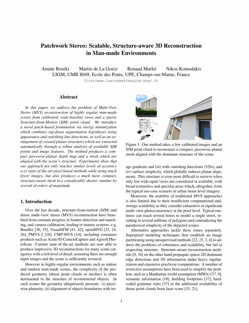
Figure 1: Our method takes a few calibrated images and an
SfM point cloud to reconstruct a compact, piecewise-planar
mesh aligned with the dominant structure of the scene.
age gradients and (iii) with vanishing directions (VDs), and
(iv) surface simplicity, which globally induces planar align-
ments. This structure is even more difficult to retrieve when
only few wide-apart views are considered or available, with
broad textureless and specular areas which, altogether, form
the typical use-case scenario in urban street-level imagery.
Moreover, the usability of traditional MVS approaches
is also limited due to their insufficient computational-and-
storage scalability as they consider exhaustive or significant
multi-view photoconsistency at the pixel level. Typical run-
times can reach several hours to model a single street, re-
sulting in several millions of polygons and contradicting the
paradoxical simplicity of the depicted scenes.
Alternative approaches tackle these issues separately.
Superpixel modeling techniques first establish an image
partitioning using unsupervised methods [22, 23, 3, 4] to ad-
dress the problems of robustness and scalability, but fail at
respecting structure. Structure-aware reconstruction meth-
ods [9, 34] on the other hand propagate sparse 2D dominant
edge detections and 3D information under heavy regular-
ization and expensive pixelwise computations. A number of
restrictive assumptions have been used to simplify the prob-
lem, such as a Manhattan-world assumption (MWA) [37, 9],
semantic information [18], building footprints [37], hard-
coded grammar rules [37] or the additional availability of
dense point clouds from laser scans [33, 21].
1
In this paper, we address the multi-view reconstruction
of structured depth maps from a few images (typically 2-5
wide-baseline images with one reference view) and a sparse
SfM point cloud (typically obtained together with image
calibration) using a scalable, region-based formulation. In
contrast to existing region-based stereo methods, ours does
not rely on a bottom-up image partitioning. Rather, we
combine vanishing directions, image contours and sparse
3D data to generate top-down segmentation hypotheses, on
which we define a Markov Random Field (MRF) topology.
The final, structured depth map is retrieved by minimizing a
global energy which groups neighboring image patches by
enforcing plausible structure-aware connectivities, resulting
in a ”patchwork” solution.
We demonstrate pixelwise accuracy results on par with
state-of-the-art dense MVS pipelines [14] while utilizing
much fewer reprojection images and gaining several orders
of magnitude in runtime and memory consumption. These
improvements are achieved thanks to both our patch-based
representation and our robust hypothesis extraction from
already-available SfM data. The resulting mesh is compact,
and aligned with scenes’ structure and image gradients by
design, which is achieved with no need of later 3D geome-
try simplification [29], nor additional complex mesh refine-
ment [39], or tedious primitive fitting steps [19].
Our main contributions are as follows:
• We propose a novel region-based stereo formula-
tion which incorporates structure priors in a princi-
pled MRF energy minimization framework where the
global energy is amenable to graph-cut inference [5].
• We define a robust joint 2D-3D method for extracting
structurally-relevant 2D line and 3D plane hypothe-
ses from principal VDs, image contours and already-
available sparse SfM data. It generates top-down su-
perpixels whose boundaries are aligned with VDs.
• We present an end-to-end pipeline which treats high-
resolution images (16MP) within a few seconds or
minutes per building, paving the way for large-scale,
compact, structure-aware urban modeling.
2. Related Work
Pixel-level MVS. A number of top-performing general
MVS algorithms assume a Delaunay tetrahedralization of
an initial 3D point cloud, whose cells are labeled with a
discrete occupancy state according to visibility and photo-
metric constraints; the reconstructed surface lies at the inter-
face between empty and non-empty cells [14, 39]. Despite
mesh refinement, the resulting surface remains a jagged
approximation of a locally-smooth geometry, which may
then require expensive post-processing to achieve a com-
pact representation, e.g., by fitting 3D geometric primi-
tives [19, 15]. The situation is even worse with voxel-based
approaches [12, 30]. Pixel-based stereo techniques, which
build disparity maps, have seen a tremendous increase in
performance since early approaches [16] and their later ex-
tensions using second order smoothness priors [40, 27],
color models [2] or semantic classification [18]. This cate-
gory of approaches has been well established for narrow-
baseline stereo problems as reported in the Middlebury
challenge [32], but it scales poorly in image number and
image size; besides, it is sensitive to wider baselines.
Superpixel modeling. Patch-based stereo approaches,
e.g., [22, 23, 3], infer piecewise-planar depth maps for su-
perpixels whose surface is assumed uniform. These super-
pixels are obtained with unsupervised bottom-up meth-
ods, that tend to randomly oversegment highly-textured re-
gions [7] and to produce hexagonal shapes in large homo-
geneous areas [1]. These methods, in comparison to pixel-
based and volumetric approaches, are more scalable and are
less sensitive to appearance, viewpoint changes and texture-
less areas. They are however completely agnostic of the
structure of the scene beyond the simple alignment of ob-
jects boundaries with image gradients, which translates into
many blatant visual artifacts. Bodis-Szomoru et al. [3] build
a multi-image graph over superpixels and reconstruct a ap-
proximate model which is very well suited for large-scale
modeling. However, patch-to-patch stereo matching adds
up to the lack of structured boundaries and alignments. It
also assumes there are enough SfM points, even in visually
homogeneous patches, which often does not hold.
Structure priors. Another line of work models weak
structure priors [34, 9] by enforcing piecewise-planarity
transitions to lie at both strong image gradients and along
edges aligned with vanishing directions. However, these are
pixelwise approaches and suffer from robustness and scal-
ability issues which restricts their usage to scenes of low
complexity and low image resolution (≤ 3MP). In contrast,
our patch-based formulation allows to handle 16MP images
with a much lower runtime by several orders of magnitude,
without assuming Manhattan scenes [9].
Top-down superpixels. Fouhey et al. [8] use a scene
representation relying on multiple top-down partitions of
an image. They intersect sets of 2D rays cast from pairs
of vanishing points, defining projective rectilinear super-
pixels/patches whose boundaries reflects their 3D orienta-
tion. The authors use this intermediate representation to es-
timate the orientation membership of each pixel in a monoc-
ular indoor Manhattan-world scene, as well as inter-patch
spatial relationships. In contrast, our approach makes use
simultaneously (vs. sequentially) of image edge detections,
vanishing directions and 3D cues from sparse SfM data to
help extract more subtle lines in a robust line-sweep stage.
Mesh alignment. Yet another line of work constructs a
mesh in the image domain, and then reconstructs vertices in
3D. Saxena et al. [31] use supervised learning to correlate
image region appearance with depth information and are
able to retrieve a plausible 3D mesh from a single calibrated
image for scenes that present a low variation of aspect and
structure. Bodis-Szomoru et al. [4] address the problem of
3D reconstruction from a single image with sparse SfM data
by triangulating superpixels [7] in the image domain, and
then fitting triangles onto SfM points by penalizing surface
curvature. The depth information of triangles with no sparse
3D information is linearly interpolated. This simplifying
assumption is made at the expense of geometric accuracy.
The rendered reconstructions can be visually satisfactory
at a coarse level for nearly flat objects and buildings (e.g.,
Haussmannian architecture), but cannot model more com-
plex yet ubiquitous elements such as protruding balconies
and loggia recesses, especially for patches with low point
density. In contrast, our method benefits from sparse SfM
cues (where available) and multi-view photoconsistency; it
propagates structurally plausible surface associations by fa-
voring planar continuity and crease junctions.
3. Overview
Inputs/Outputs. Our method takes a collection of un-
ordered calibrated images (one serving as reference, I, the
others for reprojection) and a sparse SfM point cloud S(given together with calibration information). It produces a
structured depth map and a corresponding structured mesh
for each reference image. Our notion of structure refers to
the following properties w.r.t. the expected output geom-
etry: (i) piecewise-planarity, (ii)+(iii) alignment of object
boundaries with strong image gradients and main vanishing
directions, (iv) non-local planar and boundary alignments.
Top-down segmentation and 3D plane hypotheses.
Our method first computes the dominant VDs visible in Ivia a greedy procedure. Top-down superpixels are then gen-
erated by creating in I an arrangement of dominant vanish-
ing lines (VLs). Intuitively, VLs play a key role in capturing
the layout of a regular scene as they are plausible indicators
of geometric transitions. In order to extract plane candidates
consistent with patch boundaries, i.e., to favor crease planar
transitions in 3D, VLs and dominant planes must be mutu-
ally consistent and aligned. To this end, we extract the 3D
hypotheses in a robust vanishing-line-sweeping stage which
simultaneously takes into account image features along VLs
and sparse 3D data (cf. Section 4).
MRF-Energy minimization. Our energy combines all
patches in 3D by enforcing structurally-sound associations
in accordance with multi-view patch-wise photoconsistency
and SfM cues. It is minimized efficiently (cf. Section 5).
Compact, structured mesh generation. Once the fi-
nal depth map is recovered, we generate a polygonal mesh
for each planar region. This is carried out in the image do-
main with a 2D Constrained Delaunay Triangulation (CDT)
which is then reprojected to 3D (cf. Section 6).
4. 2D Segmentation and 3D Plane Hypotheses
4.1. Estimating Vanishing Directions
As a first step, we extract dominant VDs visible in refer-
ence view I. Contrary to [34], we do not merge or cluster
them from different images as it would introduce inaccura-
cies due to calibration imprecision. It could also introduce
directions which are irrelevant in the image of interest. We
proceed as follows, without MWA, as opposed to [9, 23]:
First, we detect line segments, using LSD [38], and keep
the segments with the best scores (lowest − log(NFA)). In
our experiments, keeping the top 2500 segments of suffi-
cient length (40 pixels), we get enough cues for detecting
vanishing points (VPs) with negligible outliers.
Second, we estimate VDs. We use the VP detector of
Lezama et al. [20], which handles both Manhattan and non-
Manhattan cases. As most non-Manhattan architectures yet
include 3 Manhattan directions, we first use the Manhattan
prior and seek 3 initial Manhattan VDs. We then greedily
detect new VDs without the Manhattan prior, putting aside
associated lines at each iteration and discarding VDs too
close from previous ones (≤ 5 deg), until no more VD is
detected. This strategy allows to better retrieve VDs that
have subtle sets of supporting evidence. It may yield more
than 3 VDs, which may or may not be orthogonal.
4.2. Dominant Planes
We extract plane hypotheses in two stages. First, dom-
inant planes are detected from both the VPs and the point
cloud S . Next, more subtle planes associated to creases and
fine structural details are detected (e.g., window frames).
Concretely, we first discretize the set of plane orienta-
tions by considering VP pairs ~vi, ~vj and the associated plane
normal ~nij , given the intrinsic calibration matrix K [13]:
(1)~nij =K⊤~vi × ~vj
||K⊤~vi × ~vj ||
Then, for each ~nij , we look for associated plane offsets
(signed distance to the camera) that correspond to dominant
planes. For this, each point s∈S votes in a 1D weighted
histogram (specific to ~nij) in the bin associated to its offset.
The weight is |~nij .~ns| where ~ns is the normal of a plane
estimated by PCA analysis from points in a local neigh-
borhood N(s). To limit quantization issues in presence of
sparse regions in S , we define N(s) as the ball whose radius
is half the distance to the k-th nearest neighbor of s [28]. (In
our experiments, k=50.) The size of a bin is defined as:
(2)g = minij
(medians∈S(mij(s)))
where mij(s) is the median of the offsets of points in N(s)w.r.t. ~nij . In our experience, g provides a stable granular-
ity scale throughout different datasets; all dominant planes
are retrieved as the maxima of the histogram, unless data is
missing, e.g., due to the lack of texture.

Figure 2: VLs swept from each VP (bottom row). Pixels sup-
porting dominant VLs (top row), based on gradient features.
4.3. Dominant Vanishing Lines
We extract dominant VLs in I as lines with strong and
consistent edge information, in the following way.
We first reduce texture sensitivity by applying a bilateral
filter (σr =130, σd =3 in experiments). We then filter the
image using a Canny-Deriche edge detector [6] with double
hysteresis thresholding, resulting in a binary image Γ. To
retrieve more subtle contours, we actually extract edges at
multiple image scales (0.5, 0.75, 1 in our implementation)
and merge in Γ the resulting edge maps with a logical-or.
Then, for each VP, we sweep a VL on the binary edge
map. The fixed angular deviation between two successive
VLs is the smallest angle among the 4 angles correspond-
ing to 1 pixel of deviation at the 4 image corners. For each
swept VL l, we consider the rasterized chain of binary pix-
els it contains. For robustness, we initially apply a 1D Gaus-
sian (with σ=1), re-binarizing the line (with threshold 0.8).
For consistency, we only keep as meaningful in Γ continu-
ous chains of pixels of length at least 40. Resulting seg-
ments are illustrated on Fig. 2. Finally, dominant VLs are
defined as the local maxima of the following score:
(3)domVL(l) =1
|l|
∑
x∈l
Γ(x, l)
4.4. Secondary Lines and Planes
Leveraging on dominant planes and VL information, we
extract more subtle lines and planes. We consider the fol-
lowing three additional cues, based on creaseness.
For each dominant plane Πij with normal ~nij , for each
VP ~vk other than ~vi, ~vj , and for each VL l swept from ~vi(then symmetrically from ~vj), we consider a hypothetical
plane Πikl defined by the normal ~nik and the offset s.t. Πikl
and Πij intersect in 3D on a line L which reprojects as l. To
assess this hypothesis, we measure the following cues:
• ridgeijk(l) is the number of points in S that lie in
the slice of space at distance at most g of Πikl. It
is illustrated as the stripe between the green lines in
Figure 3: 2D-3D VL sweeping to extract secondary lines
and planes (left). Top view of SfM point cloud (right) with
regions to measure ridge cues (green), volumic points (red)
and plane junctions (purple). Please see text for details.
Fig. 3. As we only want to assess the crease hypoth-
esis at l, each point in the slice actually contributes
in creaseijk(l) according to its distance d to L, with
weight exp(−d/(40g)).
• volumij(l) is the number of “volumic” points in S that
lie in a cylinder at distance at most g of L. It is illus-
trated as the disk inside the red circle in Fig. 3. “Volu-
mic” points are considered not to lie on a line or plane,
which would not correspond to a crease. The dimen-
sionality of a point s∈S is given by PCA analysis of
neighborhood N(s). It is “volumic” if the 3 largest
eigenvalues e1, e2, e3 are comparable: 0.35 e1 ≤ e2, e3.
• junct ijk(l) is the number of points lying in a rectangu-
lar cuboid centered on L with length 8g along ~vj and
width 2g along ~vk. It is illustrated as the area inside
the purple rectangle in Fig. 3. It tells whether domi-
nant plane Πij could have a junction with Πikl at L.
Last, if junct ijk(l) ≥ 2, we consider the following score:
(4)creaseijk(l) = domVL(l) ridgeijk(l) volumij(l)
The local maxima of creaseijk(l) indicate secondary planes
Πijk and vanishing lines l.
4.5. Segmentation into Patches
The “patchwork”, i.e., the final top-down segmentation
into patches p ∈ P , is the 2D arrangement made from dom-
inant and secondary VLs, from which we discard periph-
eral patches. We only keep patches in the intersection of
regions inside the two extreme VLs extracted for each VP.
The fact is that peripheral patches often consist of sky, veg-
etation, ground or clutter pixels, which are not planar. Be-
sides, as not all vanishing orientations are represented at the
periphery (in terms of patch boundaries), it could disfavor
certain planes during inference, which could propagate by
local regularization, altering proper plane assignment.
This simple region clipping automatically restrains the
focus of the reconstruction on the main objects of interest.
It generally defines a convex hull (unless a VP lies in the
image). When a convex piecewise-planar structure is ob-
served, this strategy yields a meaningful segmentation, not
requiring manual masking [23] nor semantic or planarity
classifiers [11]. When it forms a concave region, our as-
sumption still restricts possible detrimental behaviors to the
patches that constitute the concave fraction. Our method is
however little sensitive to noise and outliers.
5. Patch-Based Stereo Revisited
We define a pairwise MRF over the graph G = (P,N )where P is the set of patches in Sect. 4.5 and N is the neigh-
borhood system of pairs of patches sharing a boundary. Let
L = {(~n1, d1), . . . , (~nN , dN )} be the label space of random
variables yp; (~np, dp) represents a plane, uniquely charac-
terized by its normal ~np and signed offset dp.
Our goal is to infer for all patches p∈P the plane assign-
ment yp with the lowest energy. The energy E(y) encour-
ages planar continuity and crease junctions, over structure
disruptions and implausible planar compositions (regular-
ization). It also favors photoconsistency between views at
patch level and adherence to the sparse SfM points (data
terms). It is defined as follows:
(5)
E(y) =∑
p∈P
wp (ΦPhotop (yp) + Φ3D
p (yp))
︸ ︷︷ ︸
Data terms
+ λ∑
(p,q)∈N
wpq ΨConnectivitypq (yp, yq)
︸ ︷︷ ︸
Regularization term
where λ balances the contribution of the unary and pairwise
potentials, and wp, wpq are adaptive normalizing weights:
(6)wp = areaI(p). exp
(
−σ(Sp)
0.1
)
where areaI(p) is the area of p, and σ(Sp) is the surface
variation of the 3D points reprojecting in p, as defined
in [28]. This value ranges between 0 (totally planar) and
1/3 (isotropically distributed points).
(7)wpq = |p ⊓ q|.max
(
0.01,1
|p ⊓ q|
∑
x∈p⊓q
µ(x)
)
where |p ⊓ q| is the length of the common edge boundary
between p and q, and µ(x) is the edge magnitude at pixel x.
The different potential functions are detailed below.
5.1. Data Terms
Multi-view photoconsistency. ΦPhotop (yp) penalizes ap-
pearance dissimilarities between a patch p and its reprojec-
tion πv(p) in other views v ∈V , assuming plane-induced
homographies [13]. For regions not reprojecting entirely
a) Planar continuity c) Plausible Occlusion (1)
b) Crease junction d) Plausible Occlusion (2)
Figure 4: The four pairwise associations modeled by our
regularization term. Surface hypotheses are represented
with boundaries aligned with a vanishing directions defin-
ing their 3D orientations. Best viewed in color.
within v, the penalty is a constant. This function is sub-
divided into an intra-patch photoconsistency and a bound-
ary edge consistency operating on patch boundary pixels Bp
and their reprojection πv(Bp).
ΦPhotop (yp) =
1|V|
∑
v∈V
{α∆(p, πv(p)) + βA(Bp, πv(Bp))}
(8)
where α, β are model parameters, and A(., .) measures the
proportion of boundary pixels agreeing on the presence of
image gradient across views. ∆(., .) is a dissimilarity func-
tion between two image regions related by homography. We
consider the zero-mean normalized cross-correlation zncc
with exponential normalization for robustness:
(9)∆(p, πv(p)) = 1− exp{−δ2
0.8}
where(10)δ = 1−max{0, zncc(p, πv(p))}
3D point consistency. We use the sparse 3D cues to encour-
age surfaces to fit onto SfM points that reproject within p:
(11)Φ3Dp (yp) = 1− exp{
−φ2
0.3}
where
(12)φ =γ
τ.|Sp|
∑
s∈Sp
min(τ,D(s, yp)
g)
where γ is a model parameter, Sp is the subset of SfM points
reprojecting within p, τ is a distance threshold (measured in
g units), and D(s, yp) is the point-to-plane 3D distance.
5.2. Regularization
Representing 3D orientations by using vanishing points
(Eq. (1)) suggests that two planar surfaces oriented resp. to-
wards ~nij and ~nij′ are likely to intersect in the image plane
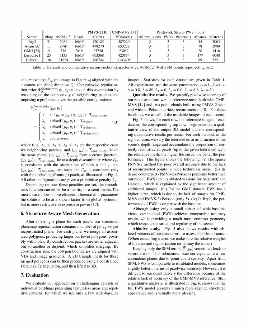
PMVS-2 [10] CMP-MVS[14] Patchwork Stereo (PWS = ours)
Scenes #Img #SfM / I Resol. #Points #Triangles #Reproj.views #VDs #Normals #Planes #Patches
Bry2 31 2081 16MP 470185 587220 2 3 3 45 2003
AugusteC 11 2980 16MP 498270 653228 3 3 3 78 2980
GMU [23] 5 578 2MP 25750 23057 3 3 3 28 1416
Lecourbe1 23 5135 16MP 603368 423854 3 3 3 177 6048
Hameau 36 21824 16MP 766744 1143405 3 3 3 89 5351
Table 1: Datasets and comparative reconstruction characteristics. #SfM/I: # of SFM points reprojecting on I.
at a crease edge ~epq (in orange in Figure 4) aligned with the
common vanishing direction ~vi. Our pairwise regulariza-
tion prior ΨConnectivitypq (yp, yq) relies on this assumption by
reasoning on the connectivity of neighboring patches and
imposing a preference over the possible configurations:
(13)
ΨConnectivitypq (yp, yq)
=
0 : if yp = yq, (yp, yq) ∈ Tcontinuity
λ1 : elseif (yp, yq) ∈ Tcrease
λ2 : elseif (yp, yq) ∈ Tocclusion1
λ3 : elseif (yp, yq) ∈ Tocclusion2
λ4 : otherwise
where 0 ≤ λ1 ≤ λ2 ≤ λ3 ≤ λ4 are the respective costs
for neighboring patches, and (yp, yq)∈Tcontinuity lie on
the same plane, (yp, yq)∈Tcrease form a crease junction,
(yp, yq)∈Tocclusion1lie at a depth discontinuity where ~epq
is consistent with the orientations of both p and q, and
(yp, yq)∈Tocclusion2are such that ~epq is consistent only
with the occluding (fronting) patch, as illustrated in Fig. 4.
All other configurations are given a prohibitive penalty λ4.
Depending on how these penalties are set, the smooth-
ness function can either be a metric, or a semi-metric.The
metric case allows more efficient inference as it guarantees
the solution to be at a known factor from global optimum,
but is more restrictive in expressive power [17].
6. Structure-Aware Mesh Generation
After inferring a plane for each patch, our structured
planemap representation contains a number of polygons per
reconstructed plane. For each plane, we merge all associ-
ated polygons, producing larger but fewer polygons, possi-
bly with holes. By construction, patches are either adjacent
one to another or disjoint, which simplifies merging. By
construction also, the polygon boundaries are aligned with
VDs and image gradients. A 2D triangle mesh for these
merged polygons can be then produced using a constrained
Delaunay Triangulation, and then lifted to 3D.
7. Evaluation
We evaluate our approach on 5 challenging datasets of
individual buildings presenting textureless areas and repet-
itive patterns, for which we use only a few wide-baseline
images. Statistics for each dataset are given in Table 1.
All experiments use the same parameters: α=1, β=0.4,
γ=0.5, λ=30, λ1 =0, λ2 =0.6, λ3 =3.8, λ4 =50.
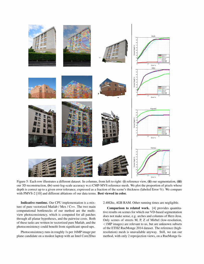
Quantitative results. We quantify pixelwise accuracy of
our reconstructions w.r.t. a reference mesh built with CMP-
MVS [14] and two point clouds built using PMVS-2 with
and without Poisson surface reconstruction [10]. For these
baselines, we use all of the available images of each scene.
Fig. 5 shows, for each row, the reference image of each
dataset, the corresponding top-down segmentation, a qual-
itative view of the output 3D model and the correspond-
ing quantitative results per scene. For each method, in the
right column, we vary the tolerated error as a fraction of the
scene’s depth range and accumulate the proportion of cor-
rectly reconstructed pixels (up to the given tolerance) w.r.t.
the reference mesh; the higher the curve, the better the per-
formance. This figure shows the following: (i) The sparse
PMVS-2 method has poor overall accuracy due to the lack
of reconstructed points in wide textureless areas. (ii) Its
dense counterpart (PMVS-2+Poisson) performs better than
our model (PWS) and its ablated versions for AugusteC and
Hameau, which is explained by the significant amount of
additional images. (iii) For the GMU dataset, PWS has a
higher curve, which is due to the lack of images for CMP-
MVS and PMVS-2+Poisson (only 5). (iv) In Bry2, the per-
formance of PWS is on par with the baseline.
Although using only a small subset of wide-baseline
views, our method (PWS) achieves comparable accuracy
results while providing a much more compact geometry
which respects the structural regularity of the scene.
Ablative study. Fig. 5 also shows results with ab-
lated variants of our data terms, to assess their importance.
(When cancelling a term, we make sure the relative weights
of the data and regularization terms stay the same.)
Keeping only the SFM term Φ3Dp (yp) sometimes leads to
severe errors. This robustness issue corresponds to a few
anomalous planes due to point could sparsity. Apart from
SFM, PWS is comparable to its ablated models, sometimes
slightly better in terms of pixelwise accuracy. However, it is
difficult to see quantitatively the difference because of the
relative lack of accuracy of the CMP-MVS reference. Still,
a qualitative analysis, as illustrated in Fig. 6, shows that the
full PWS model presents a much more regular, structured
appearance and is visually more pleasing.
10−1
100
101
102
0
10
20
30
40
50
60
70
80
90
100
Error %
Corr
ect
Depth
%
Bry2b
PWS (Ours)
PMVS−2
PMVS−2+Poisson
Photo only
SFM only
Photo+Edge
Photo+SFM
10−1
100
101
102
0
10
20
30
40
50
60
70
80
90
100
Error %
Corr
ect
Depth
%
GMU
PWS (Ours)
PMVS−2
PMVS−2+Poisson
Photo only
SFM only
Photo+Edge
Photo+SFM
10−1
100
101
102
0
10
20
30
40
50
60
70
80
90
100
Error %
Corr
ect D
epth
%
AugusteC
PWS (Ours)
PMVS−2
PMVS−2+Poisson
Photo only
SFM only
Photo+Edge
Photo+SFM
10−1
100
101
102
0
10
20
30
40
50
60
70
80
90
100
Error %
Corr
ect D
epth
%
Hameau
PWS (Ours)
PMVS−2
PMVS−2+Poisson
Photo only
SFM only
Photo+Edge
Photo+SFM
Figure 5: Each row illustrates a different dataset. In columns, from left to right: (i) reference view, (ii) our segmentation, (iii)
our 3D reconstruction, (iv) semi-log-scale accuracy w.r.t CMP-MVS reference mesh. We plot the proportion of pixels whose
depth is correct up to a given error tolerance, expressed as a fraction of the scene’s thickness (labeled Error %). We compare
with PMVS-2 [10] and different ablations of our data terms. Best viewed in color.
Indicative runtime. Our CPU implementation is a mix-
ture of pure vectorized Matlab / Mex / C++. The two main
computational bottlenecks of our method are the multi-
view photoconsistency, which is computed for all patches
through all planar hypotheses, and the pairwise costs. Both
of these tasks are written in vectorized pure Matlab, and the
photoconsistency could benefit from significant speed-ups.
Photoconsistency runs in roughly 1s per 16MP image per
plane candidate on a modest laptop with an Intel Core2Duo
2.40Ghz, 4GB RAM. Other running times are negligible.
Comparison to related work. [4] provides quantita-
tive results on scenes for which our VD-based segmentation
does not make sense, e.g. arches and columns of Herz-Jesu.
Only scenes of streets M, P, Z of Mirbel (low-resolution,
<1MP images) are relevant to us, but are unknown subsets
of the ETHZ RueMonge 2014 dataset. The reference (high-
resolution) mesh is unavailable anyway. Still, we ran our
method, with only 2 reprojection views, on a RueMonge fa-
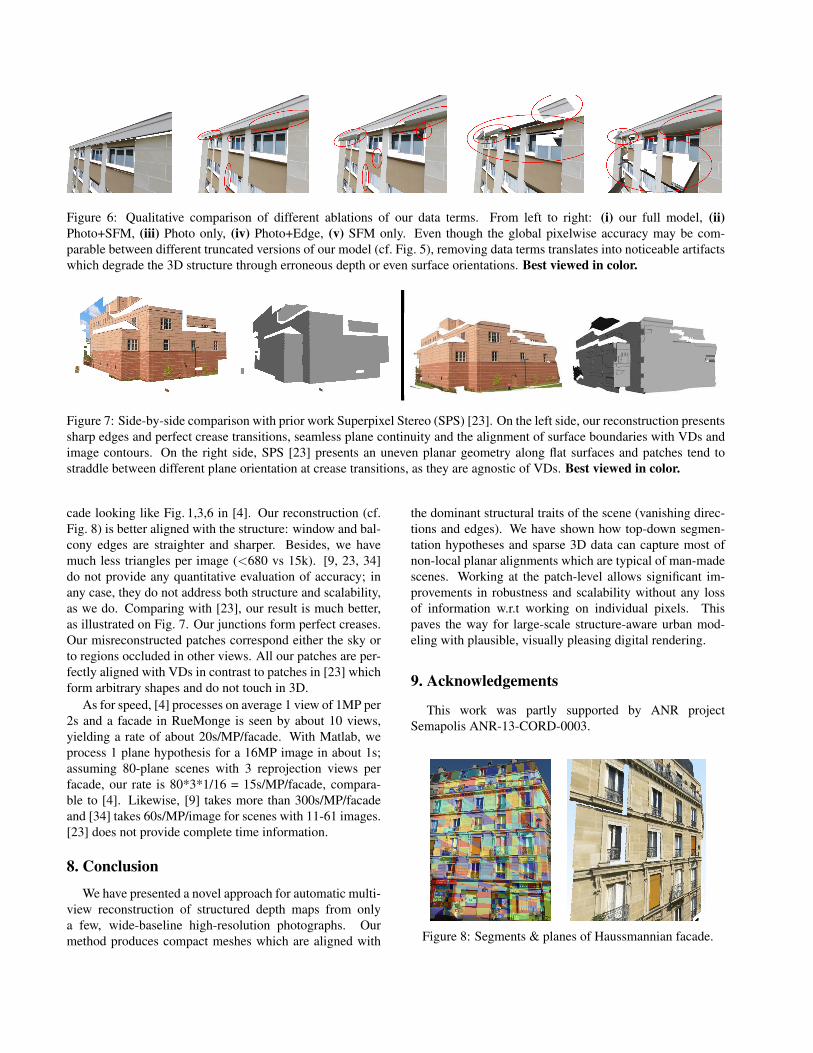
Figure 6: Qualitative comparison of different ablations of our data terms. From left to right: (i) our full model, (ii)
Photo+SFM, (iii) Photo only, (iv) Photo+Edge, (v) SFM only. Even though the global pixelwise accuracy may be com-
parable between different truncated versions of our model (cf. Fig. 5), removing data terms translates into noticeable artifacts
which degrade the 3D structure through erroneous depth or even surface orientations. Best viewed in color.
Figure 7: Side-by-side comparison with prior work Superpixel Stereo (SPS) [23]. On the left side, our reconstruction presents
sharp edges and perfect crease transitions, seamless plane continuity and the alignment of surface boundaries with VDs and
image contours. On the right side, SPS [23] presents an uneven planar geometry along flat surfaces and patches tend to
straddle between different plane orientation at crease transitions, as they are agnostic of VDs. Best viewed in color.
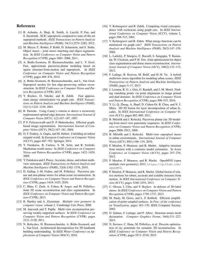
cade looking like Fig. 1,3,6 in [4]. Our reconstruction (cf.
Fig. 8) is better aligned with the structure: window and bal-
cony edges are straighter and sharper. Besides, we have
much less triangles per image (<680 vs 15k). [9, 23, 34]
do not provide any quantitative evaluation of accuracy; in
any case, they do not address both structure and scalability,
as we do. Comparing with [23], our result is much better,
as illustrated on Fig. 7. Our junctions form perfect creases.
Our misreconstructed patches correspond either the sky or
to regions occluded in other views. All our patches are per-
fectly aligned with VDs in contrast to patches in [23] which
form arbitrary shapes and do not touch in 3D.
As for speed, [4] processes on average 1 view of 1MP per
2s and a facade in RueMonge is seen by about 10 views,
yielding a rate of about 20s/MP/facade. With Matlab, we
process 1 plane hypothesis for a 16MP image in about 1s;
assuming 80-plane scenes with 3 reprojection views per
facade, our rate is 80*3*1/16 = 15s/MP/facade, compara-
ble to [4]. Likewise, [9] takes more than 300s/MP/facade
and [34] takes 60s/MP/image for scenes with 11-61 images.
[23] does not provide complete time information.
8. Conclusion
We have presented a novel approach for automatic multi-
view reconstruction of structured depth maps from only
a few, wide-baseline high-resolution photographs. Our
method produces compact meshes which are aligned with
the dominant structural traits of the scene (vanishing direc-
tions and edges). We have shown how top-down segmen-
tation hypotheses and sparse 3D data can capture most of
non-local planar alignments which are typical of man-made
scenes. Working at the patch-level allows significant im-
provements in robustness and scalability without any loss
of information w.r.t working on individual pixels. This
paves the way for large-scale structure-aware urban mod-
eling with plausible, visually pleasing digital rendering.
9. Acknowledgements
This work was partly supported by ANR project
Semapolis ANR-13-CORD-0003.
Figure 8: Segments & planes of Haussmannian facade.
References
[1] R. Achanta, A. Shaji, K. Smith, A. Lucchi, P. Fua, and
S. Susstrunk. SLIC superpixels compared to state-of-the-art
superpixel methods. IEEE Transactions on Pattern Analysis
and Machine Intelligence (PAMI), 34(11):2274–2282, 2012.
[2] M. Bleyer, C. Rother, P. Kohli, D. Scharstein, and S. Sinha.
Object stereo – joint stereo matching and object segmenta-
tion. In IEEE Conference on Computer Vision and Pattern
Recognition (CVPR), pages 3081–3088, 2011.
[3] A. Bodis-Szomoru, H. Riemenschneider, and L. V. Gool.
Fast, approximate piecewise-planar modeling based on
sparse structure-from-motion and superpixels. In IEEE
Conference on Computer Vision and Pattern Recognition
(CVPR), pages 469–476, 2014.
[4] A. Bodis-Szomoru, H. Riemenschneider, and L. Van Gool.
Superpixel meshes for fast edge-preserving surface recon-
struction. In IEEE Conference on Computer Vision and Pat-
tern Recognition (CVPR), 2015.
[5] Y. Boykov, O. Veksler, and R. Zabih. Fast approxi-
mate energy minimization via graph cuts. IEEE Transac-
tions on Pattern Analysis and Machine Intelligence (PAMI),
23(11):1222–1239, 2001.
[6] R. Deriche. Using Canny’s criteria to derive a recursively
implemented optimal edge detector. International Journal of
Computer Vision (IJCV), 1(2):167–187, 1987.
[7] P. F. Felzenszwalb and D. P. Huttenlocher. Efficient graph-
based image segmentation. International Journal of Com-
puter Vision (IJCV), 59(2):167–181, 2004.
[8] D. F. Fouhey, A. Gupta, and M. Hebert. Unfolding an indoor
origami world. In European Conference on Computer Vision
(ECCV), pages 687–702. Springer, 2014.
[9] Y. Furukawa, B. Curless, S. M. Seitz, and R. Szeliski.
Manhattan-world stereo. In IEEE Conference on Computer
Vision and Pattern Recognition (CVPR), pages 1422–1429,
2009.
[10] Y. Furukawa and J. Ponce. Accurate, dense, and robust multi-
view stereopsis. IEEE Transactions on Pattern Analysis and
Machine Intelligence (PAMI), 32(8):1362–1376, 2010.
[11] D. Gallup, J.-M. Frahm, and M. Pollefeys. Piecewise pla-
nar and non-planar stereo for urban scene reconstruction. In
IEEE Conference on Computer Vision and Pattern Recogni-
tion (CVPR), pages 1418–1425, 2010.
[12] C. Hane, C. Zach, A. Cohen, R. Angst, and M. Pollefeys.
Joint 3D scene reconstruction and class segmentation. In
IEEE Conference on Computer Vision and Pattern Recogni-
tion (CVPR), 2013.
[13] R. Hartley and A. Zisserman. Multiple view geometry in
computer vision, volume 2. Cambridge Univ Press, 2000.
[14] M. Jancosek and T. Pajdla. Multi-view reconstruction pre-
serving weakly-supported surfaces. In IEEE Conference on
Computer Vision and Pattern Recognition (CVPR), pages
3121–3128, 2011.
[15] N. Kobyshev, H. Riemenschneider, A. Bodis-Szomoru, and
L. Van Gool. Architectural decomposition for 3D landmark
building understanding. In IEEE Winter Conference on Ap-
plications of Computer Vision (WACV), 2016.
[16] V. Kolmogorov and R. Zabih. Computing visual correspon-
dence with occlusions using graph cuts. In IEEE Interna-
tional Conference on Computer Vision (ICCV), volume 2,
pages 508–515, 2001.
[17] V. Kolmogorov and R. Zabin. What energy functions can be
minimized via graph cuts? IEEE Transactions on Pattern
Analysis and Machine Intelligence (PAMI), 26(2):147–159,
2004.
[18] L. Ladicky, P. Sturgess, C. Russell, S. Sengupta, Y. Bastan-
lar, W. Clocksin, and P. H. Torr. Joint optimization for object
class segmentation and dense stereo reconstruction. Interna-
tional Journal of Computer Vision (IJCV), 100(2):122–133,
2012.
[19] F. Lafarge, R. Keriven, M. Brdif, and H.-H. Vu. A hybrid
multiview stereo algorithm for modeling urban scenes. IEEE
Transactions on Pattern Analysis and Machine Intelligence
(PAMI), pages 5–17, 2013.
[20] J. Lezama, R. G. v. Gioi, G. Randall, and J.-M. Morel. Find-
ing vanishing points via point alignments in image primal
and dual domains. In IEEE Conference on Computer Vision
and Pattern Recognition (CVPR), pages 509–515, 2014.
[21] Y. Li, Q. Zheng, A. Sharf, D. Cohen-Or, B. Chen, and N. J.
Mitra. 2D-3D fusion for layer decomposition of urban fa-
cades. In IEEE International Conference on Computer Vi-
sion (ICCV), pages 882–889, 2011.
[22] B. Micusık and J. Kosecka. Piecewise planar city 3D model-
ing from street view panoramic sequences. In IEEE Confer-
ence on Computer Vision and Pattern Recognition (CVPR),
pages 2906–2912, 2009.
[23] B. Micusık and J. Kosecka. Multi-view superpixel stereo
in urban environments. International Journal of Computer
Vision (IJCV), 89(1):106–119, 2010.
[24] P. Moulon, P. Monasse, and R. Marlet. Adaptive structure
from motion with a contrario model estimation. In Asian
Conference on Computer Vision (ACCV), pages 257–270,
2012.
[25] P. Moulon, P. Monasse, and R. Marlet. OpenMVG (open
multiple view geometry), 2012. https://github.com/
openMVG.
[26] P. Moulon, P. Monasse, and R. Marlet. Global fusion of rela-
tive motions for robust, accurate and scalable structure from
motion. In IEEE International Conference on Computer Vi-
sion (ICCV), pages 3248–3255, 2013.
[27] C. Olsson, J. Ulen, and Y. Boykov. In defense of 3D-label
stereo. In IEEE Conference on Computer Vision and Pattern
Recognition (CVPR), pages 1730–1737, 2013.
[28] M. Pauly, M. Gross, and L. P. Kobbelt. Efficient simplifi-
cation of point-sampled surfaces. In Proc. of the conference
on Visualization, pages 163–170. IEEE Computer Society,
2002.
[29] D. Salinas, F. Lafarge, and P. Alliez. Structure-aware mesh
decimation. Computer Graphics Forum, 34(6):211–227,
2015.
[30] N. Savinov, C. Hane, M. Pollefeys, et al. Discrete optimiza-
tion of ray potentials for semantic 3D reconstruction. In
IEEE Conference on Computer Vision and Pattern Recog-
nition (CVPR), pages 5511–5518, 2015.
[31] A. Saxena, M. Sun, and A. Y. Ng. Make3D: Learning 3D
scene structure from a single still image. IEEE Transac-
tions on Pattern Analysis and Machine Intelligence (PAMI),
31(5):824–840, 2009.
[32] D. Scharstein and R. Szeliski. A taxonomy and evaluation
of dense two-frame stereo correspondence algorithms. Inter-
national Journal of Computer Vision (IJCV), 47(1-3):7–42,
2002.
[33] C.-H. Shen, S.-S. Huang, H. Fu, and S.-M. Hu. Adaptive par-
titioning of urban facades. ACM Transactions on Graphics
(TOG), 30(6):184, 2011.
[34] S. N. Sinha, D. Steedly, and R. Szeliski. Piecewise pla-
nar stereo for image-based rendering. In IEEE International
Conference on Computer Vision (ICCV), pages 1881–1888,
2009.
[35] N. Snavely. Bundler: Structure from motion (SfM) for un-
ordered image collections, 2010. v0.4, http://www.cs.
cornell.edu/\verb+˜+snavely/bundler.
[36] N. Snavely, S. Seitz, and R. Szeliski. Photo tourism: Explor-
ing image collections in 3D. ACM Transactions on Graphics
(TOG), 25(3):835–846, July 2006.
[37] C. A. Vanegas, D. G. Aliaga, and B. Benevs. Building recon-
struction using Manhattan-world grammars. IEEE Confer-
ence on Computer Vision and Pattern Recognition (CVPR),
0:358–365, 2010.
[38] R. G. von Gioi, J. Jakubowicz, J.-M. Morel, and G. Randall.
LSD: a fast line segment detector with a false detection con-
trol. IEEE Transactions on Pattern Analysis and Machine
Intelligence (PAMI), 32(4):722–732, 2008.
[39] H.-H. Vu, P. Labatut, J.-P. Pons, and R. Keriven. High accu-
racy and visibility-consistent dense multiview stereo. IEEE
Transactions on Pattern Analysis and Machine Intelligence
(PAMI), 34(5):889–901, 2012.
[40] O. Woodford, P. Torr, I. Reid, and A. Fitzgibbon. Global
stereo reconstruction under second-order smoothness priors.
IEEE Transactions on Pattern Analysis and Machine Intelli-
gence (PAMI), 31(12):2115–2128, 2009.
[41] C. Wu. VisualSFM: A visual structure from motion system,
2011. http://ccwu.me/vsfm.
[42] C. Wu. Towards linear-time incremental structure from mo-
tion. In IEEE International Conference on 3D Vision (3DV),
pages 127–134, 2013.