Structural health monitoring

Tomonori NagayamaTomonori NagayamaAssistant professor University of Tokyo

/ /2010/07/19

Introduction

Civil infrastructureV l bl t hi h k d liValuable asset, which keeps economy and lives running

l b d ( k h k d )A long span bridge (ex. Akashi‐Kaikyo Bridge in Japan) costs billions of dollarsG ld G t B id h ~ 40 illi iGolden Gate Bridge has ~ 40 million crossing per year

2

Degrading infrastructure

>40 % of the nation’s bridges are structurally deficient or functionally obsolete (FHWAdeficient or functionally obsolete (FHWA, sufficiency rating) >800 l b id i th ti l b id>800 long span bridges in the national bridge inventory (NBI) are fracture‐critical.

3

Maintenance is vital

schedule‐driven, or based on expensive and questionable visual inspectionquestionable visual inspection

Inspections Every two years for >600 000 bridges in USEvery two years for >600,000 bridges in US.Every two ‐ five years in Japan

B kl B id i l i ti >3 th >$1 illiBrooklyn Bridge visual inspection: >3month, >$1million 56% of visual inspection results are incorrect with a 95% probability (based on sample tests on inspectors)95% probability (based on sample tests on inspectors)

A t ti t f t t ’ t t t (Accurate estimate of structures’ current state (or SHM) will enable efficient and effective Condition‐B d M i t (CBM)Based Maintenance (CBM)

4

Sensory systems for structures

DiagnosticsPrognostics

Sensory

Prognostics

SensorySystem

SensorySystem

SafetyPerformance

Life-Cycle Cost y

From Prof. Spencer’s lecture

Various purposes of SHMTo monitor and control the construction processT lid t th t t l d i d h t iTo validate the structural designs and characterize performance (e.g., develop database)To characterize loads in situTo assist with building/bridge maintenanceTo detect and localize damage before it reaches a critical level, thus increasing the safety to the public, g y pTo reduce the costs and down‐time associated with repair of damagerepair of damageTo assist with emergency response efforts, including building evacuation and traffic controlbuilding evacuation and traffic control

From Prof. Spencer’s lecture

Classification into 4 levels

1. Detect damage2 Locate damage2. Locate damage3. Identify the severity of damage4 P di t th i i i lif f th t t4. Predict the remaining service life of the structure.

How? Any better alternative or complement to visual inspection?How? Any better alternative or complement to visual inspection?Static measurement‐based SHM

Ex.) static strain monitoring using fiber optic sensor.NDT for detailed inspection

Ex.) acoustic emission, ultrasonic testing, radiographic inspection, etc.i b d hImage processing‐based approach

Ex.) Crack detection from image processing.Vibration‐based SHMVibration‐based SHM

More information than static measurement.No need to measure at the surface. 7

Common practice for vibration‐based SHM

1. Vibration measurementOutput: Acceleration, Velocity, Displacement, Input force, etc.Method: Ambient vibration, Shaker excitation, etc.

2. Feature extractionModal AnalysisOutput: Natural Frequency, Damping ratio, Mode shape, etcMethod: Time Domain method, Frequency Domain method

l lStructural AnalysisOutput: Flexibility, Mass, Damping, and/or Stiffness MatricesMethod: Optimization, Stiffness or Flexibility Matrix synthesis fromMethod: Optimization, Stiffness or Flexibility Matrix synthesis from

Mass and Modal information

3. Damage Assessment

8

gOutput: Damage existence, location, severity, expected life, etc.Method: Damage Locating Vector, Change in Stiffness Matrix etc.

Vibration‐based SHM

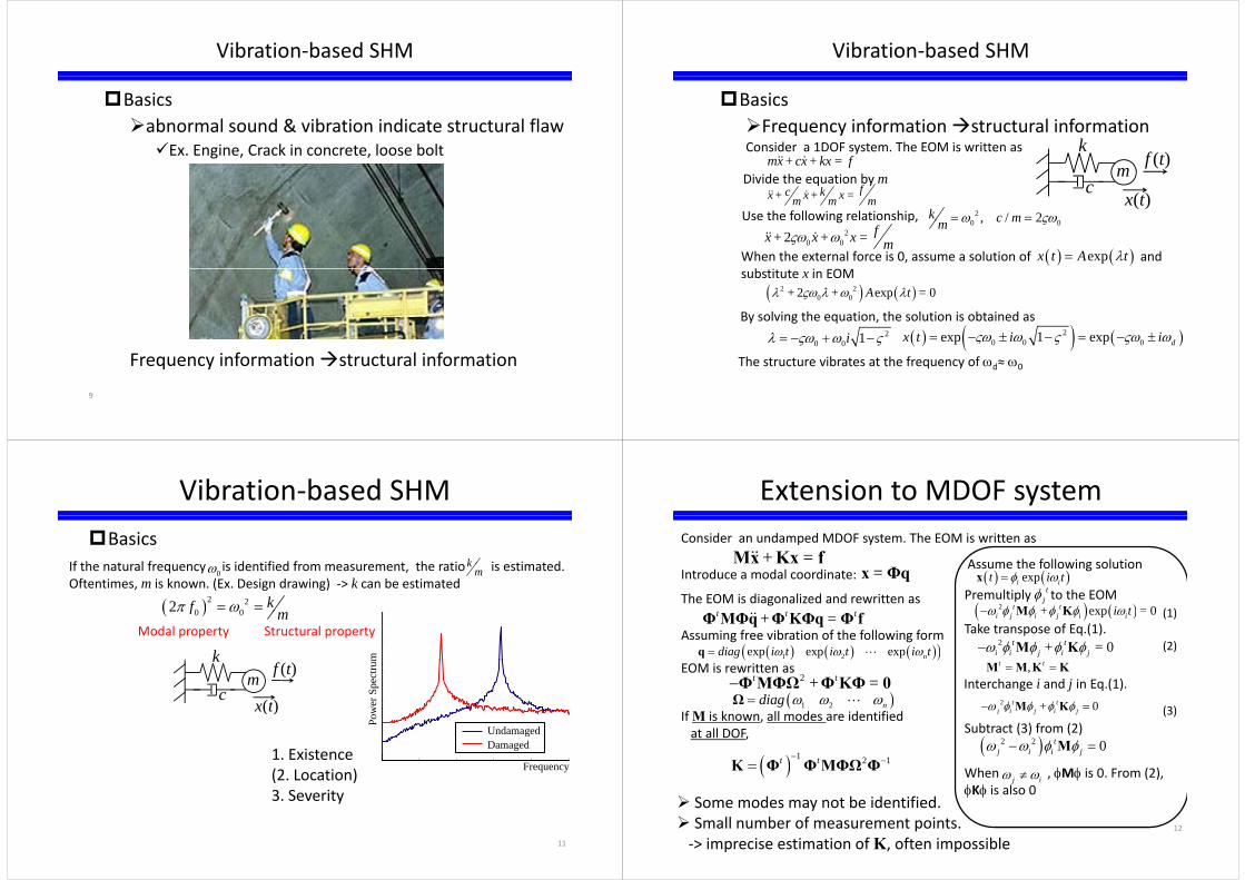
Basicsabnormal sound & vibration indicate structural flawabnormal sound & vibration indicate structural flaw

Ex. Engine, Crack in concrete, loose bolt

Frequency information structural information

9

Frequency information structural information

Vibration‐based SHM

BasicsFrequency information structural informationFrequency information structural information

mx+cx+kx = f&& &Consider a 1DOF system. The EOM is written as

mk

f (t)fc kx+ x+ x =m m m&& &

Use the following relationship, x(t)

mcDivide the equation by m

20 0/ 2= =k c mω ςω

20 02 fx+ x+ x = mςω ω&& &

g p, 0 0, / 2c mm ω ςω

When the external force is 0, assume a solution of and b

( ) ( )exp=x t A tλsubstitute x in EOM

( ) ( )2 20 02 exp 0+ + A t =λ ςω λ ω λ

By solving the equation the solution is obtained as( ) ( ) ( )2

0 0 0exp 1 exp= − ± − = − ± dx t i iςω ω ς ςω ωBy solving the equation, the solution is obtained as

20 0 1= − + −iλ ςω ω ς

The structure vibrates at the frequency of ωd≈ ω0The structure vibrates at the frequency of ωd ω0

Vibration‐based SHMBasics

If th t l f i id tifi d f t th ti i ti t dk

( )2 20 02 = = kfπ ω

If the natural frequency is identified from measurement, the ratio is estimated.Oftentimes, m is known. (Ex. Design drawing) ‐> k can be estimated

0ωk

m

m

( )0 0f mStructural propertyModal property

k

wer

Spe

ctru

m

x(t)m

c

kf (t)

UndamagedDamaged

Powx(t)

1 ExistenceFrequency

1. Existence(2. Location)3. Severity

11

Extension to MDOF system

+ =Mx Kx f&&Consider an undamped MDOF system. The EOM is written as

Assume the following solutionIntroduce a modal coordinate: =x ΦqThe EOM is diagonalized and rewritten as

t t t

( ) ( )exp= i it i tφ ωxAssume the following solution

Premultiply to the EOM tjφ

( ) ( )2 exp 0− t t+ i t =ω φ φ φ φ ωM K (1)t t t+ =Φ MΦq Φ KΦq Φ f&& ( ) ( )exp 0i j i j i i+ i tω φ φ φ φ ωM KTake transpose of Eq.(1).

(1)

2 0− t ti i j i j+ =ω φ φ φ φM K (2)( ) ( ) ( )( )1 2exp exp exp= ndiag i t i t i tω ω ωq L

Assuming free vibration of the following form

2 0− =t t+ω φ φ φ φM K

Interchange i and j in Eq.(1).

(3)

,= =t tM M K K( )

EOM is rewritten as 2− t t+ =Φ MΦΩ Φ KΦ 0

( )1 2= ndiag ω ω ωΩ L 0=j i j i j+ω φ φ φ φM K (3)Subtract (3) from (2)

( )2 2 0− =tj i i jω ω φ φM

If M is known, all modes are identified at all DOF,

( ) 1−

( )

( )When , φMφ is 0. From (2),φKφ is also 0

≠j iω ω( ) 1 2 1− −= t tK Φ Φ MΦΩ Φ

Some modes may not be identified12

Some modes may not be identified. Small number of measurement points. ‐> imprecise estimation of K, often impossible

Stiffness matrix estimation( ) 1 2 1− −= t tK Φ Φ MΦΩ Φ2− t t+ =Φ MΦΩ Φ KΦ 0

When some modes are not observed, matrix inverse cannot be calculated.2= =tΦ MΦ M vUsing , the stiffness can be written as

( ) 1 2 1− −= t tK Φ v Ω vΦAlso from definition Therefore( )2 t ( )2t

(1)Also, from definition, . Therefore, ( )2− =tv Φ M Φ I ( )2− =tΦ MΦv I

1 2− −= tΦ v Φ M ( ) 1 2− −=tΦ MΦvThe stiffness matrix can be written asThe stiffness matrix can be written as

1 2 1− −= TK MΦv Ω v Φ MConsidering that is diagonal matrix, K can be written as summation of contribution from each mode

1 2 1− −v Ω vof contribution from each mode.

2 2

1

−

=

= ∑n

Tj j j j

jvφ ω φK M M (2)

If only m modes out of n modes are observable, K has estimation error.Because frequencies appear in (2) as weighting coefficients, high

13

Because frequencies appear in (2) as weighting coefficients, high frequency modes have large influences on K

Flexibility matrix estimationFrom (1), the Flexibility matrix, F=K-1, is written as follows.

( )1 2 1− − −=t

F Φv Ω Φv( )Considering contribution from each mode, the matrix is expressed as

2 2

1

− −

=

= ∑n

tj j j j

jvφ ω φF (3)

j

If only m modes out of n modes are observable, F has estimation error.Because the reciprocal of frequencies appear in (3) as weighting coefficients,

low frequency modes have large influences on Flow frequency modes have large influences on F

14

Comparison of stiffness and flexibility matrix estimations

M d l id ifi i i f d hModal identification is performed on the truss. K and F are estimated from identified modes.

Stiffness matrix estimation Flexibility matrix estimation

error

error

timation e

timation e

Est

Est

15

Only low frequency modes provide reasonable estimation

Mass matrix may be unknown…

Δ

When mass matrix is unknown, calibrate the system using known massSuppose the frequencies of the system before and after

kf (t)m

Δm20 =m kω

Suppose the frequencies of the system before and after addition of the mass are ω0 and ω1.

( ) 2+ Δ k20

22

01⎡ ⎤− ⎧ ⎫⎧ ⎫=⎨ ⎬ ⎨ ⎬⎢ ⎥ Δ⎩ ⎭ ⎩ ⎭

mk

ω

x(t)cm( ) 2

1+ Δ =m m kω 2211 1 ⎨ ⎬ ⎨ ⎬⎢ ⎥ −Δ− ⎩ ⎭ ⎩ ⎭⎣ ⎦ mk ωω

When Δm is small, the matrix is ill‐posed.To improve the accuracy mass perturbation cases can beTo improve the accuracy, mass perturbation cases can be increased.

20 01⎡ ⎤− ⎧ ⎫

⎢ ⎥ ⎪ ⎪ω

Least Square problemMinimize the residual error of Ax = b expressed as follows

022

1 11

22

1

1

⎧ ⎫⎢ ⎥ ⎪ ⎪−Δ− ⎧ ⎫ ⎪ ⎪⎢ ⎥ =⎨ ⎬ ⎨ ⎬⎢ ⎥ ⎩ ⎭ ⎪ ⎪⎢ ⎥ ⎪ ⎪Δ⎢ ⎥ ⎩ ⎭⎣ ⎦

mmk

m

ωω

ωMM M

[ ] [ ]= − −= − − +

t

t t t t t tJ Ax b Ax b

x A Ax b Ax x A b b b

) )) ) ) )

∂J2 1 ⎪ ⎪−Δ−⎢ ⎥ ⎩ ⎭⎣ ⎦ n nn m ωω

A x = b2 2 0∂

= − =∂

t tJ A Ax A bx

))

( ) 1−= t tx A A A b)

16

( )For MDOF extension, refer to Dinh et al. (2009)

Extension to civil infrastructure

Civil infrastructure’s features:L lLarge scaleContinuous system infinite DOF or approximationinfinite DOF or approximationLarge number of elementsRedundant structureRedundant structureDistinctive designL t l fLow natural frequencyNon‐trivial input forceD i d i t il il blDesign drawing not necessarily availableetc.

Change in modal propertiesPrecise inverse estimation of structural properties are often difficultare often difficultThe existence and location of damage are sought f diff b t d l ti b ffrom differences between modal properties before and after damage.

Frequency Damping ratioMode shapes Stiffness and flexibility matricesStiffness and flexibility matrices

18

Small change in modal properties

Change in modal properties is not apparent

x&&measurement50% section loss

trum

ower

Spe

ct

UndamagedDamaged

Po

19

gFrequency

Frequency change

The vibration of a bridge on I40 was measured while progressively damaging the structureprogressively damaging the structure.

Identified natural frequencies

??

Changes in frequencies and temperature

Damage detection based on frequency changesFinding from the Rio Grande bridge experiment

The change in frequency due to damage is smallg q y gFrequency increase was observedTemperature change (thermal gradient) has

l h f hcorrelation with frequency change.

Findings from other studiesFindings from other studiesDetectability depends on modesChange in single modal frequency does not locateChange in single modal frequency does not locate damageChanges in modal frequencies may indicate damage g q y glocation

Offshore plant monitoring started earlier. The tidal variation and tank contents have large influence on the

23

variation and tank contents have large influence on the dynamic behavior. Damage detection has been considered challenging

Damage detection based on damping changes

The change is larger than changes in frequenciesAs large as 80％（Agardh １９９１）As large as 80％（Agardh １９９１）

Large damping indicates energy consumption. sign of crack and other damage?sign of crack and other damage?Difficult to modelEstimation error is large.

There are reports indicating spatial difference in damping ratios due to structural damage.

24

Damping ratio and progressive damage

??

Damage detection based on mode shape changes

Mode shape changes as structural properties changes.

i di M d l A C i i (MAC)indices：Modal Assurance Criterion (MAC)

Sensitivity to damage is not necessarily high Various mode shape based indices have been proposed.The shape near the mode shape nodeSpatial derivative of mode shapeSpatial derivative of mode shapeStrain mode shapeSensitive modes ‐> high order modesM d h hMode shape phase

limitation： The number of measurement point is limitedlimitation： The number of measurement point is limited to capture mode shapes of continuous systems.

26

Recent studies in SHM

27

Recent studies in SHM

Research in the past has not resulted in sufficient performance evaluation⇒ efforts in each stepperformance evaluation⇒ efforts in each step

Measurement Sensing d t hi h l ti

Feature extractionAcceleration, strain, velocity

displacement, etc

dense measurement, high resolution,wide frequency range

The use of seismic record, traffic induced vibration and additional mass

FrequencyDampingMode shapes

vibration and additional mass

F t l i

Mode shapesVibration amplitude

Feature analysisComparison with design,

past measurement

Damage Locating Vector methodsSimulation considering vehicle‐bridgeinteraction

28

Judgmentpast measurement

Statistical analysis/wavelet，Non‐linear model

Detailed FEMComparison among similar structures

Dense and high‐resolution sensing using Laser Doppler vibrometer

The velocity of objects is y jmeasured using the Doppler effect of the laser

Characteristics・Non‐contact → up to 100 [m] (for steel)・High resolution → 0.3 μm/s・wide frequency range → 0～35kHz・scan large spatial area (spatial information)

scan angle (+‐ 15 degree )

29

dense and high resolution non‐contact vibration measurements are feasible

Experimental verificationSteel plate(400×300×2mm)

Dense measurement by scanning

horizontal ：10 ptshorizontal ：10 pts.vertical ： 10 pts.

total：100 ptstotal：100 pts(spatially dense measurement)

Sampling frequency ： 2000Hzdata points ： 2048 p

Ambient vibration can be captured30

Ambient vibration can be captured

Steel plate mode shape

# of averaging: 10 100 300 FEM

1st mode

10 7Hz10.7Hz

14th

12.1Hz

14thmode

80580Hz

600Hz

31

600Hz

Identified mode shapes

32.23 Hz(34 18Hz)

10.74 Hz（12.07 Hz） 137.2 Hz

(135 0H )

112.8 Hz(121 0Hz)

66.89 Hz(76 01Hz)(34.18Hz) (135.0Hz)(121.0Hz)(76.01Hz)

Hi h d d lHigh order modes can also be identified

233.9Hz(234 5Hz)

345.7 Hz(336 7H )

238.8 Hz(260 9Hz)

32

(234.5Hz) (336.7Hz)(260.9Hz)

331. Long Distance Measurement for GZ New TV Tower(Under Construction) 09.01.08-09.01.14( )

広州

+Velocimeter

香港

Complete in 2009

• Using reflectors, distant measurement is feasibleg ,

Joint research with the Hong Kong Polytechnic University

Dense synchronized measurement using wireless sensors

Wireless smart sensors (WSS) allows dense and inexpensive measurements

Recent wireless smart sensor platform development

Difficulties toward full‐scale bridge vibration measurement

p p

Difficulties toward full scale bridge vibration measurementSensing capability (resolution, synchronization)Robustness (system reliability)Robustness (system reliability)Communication (RF range, packet loss)

34

Application to a full‐scale bridgeMain span 570 m49 d l h id lk49 nodes along the side walk.

Prompt installationInstallation ：90min, Removal：45min by 3 persons

Application to a fullApplication to a full‐‐scale bridgescale bridgeCable : 8Deck : 22Pylon : 3Total : 33

Cable : 8Deck : 26Pylon : 3Total : 37Total : 33 Total : 37

In total, 420 channels of sensorsIn total, 420 channels of sensors

Vibration‐Sentry

A t

0Amemometer

interfaced with Wind‐Sentry

Nodes on pylon top Nodes on cables

Structural Dynamics Laboratory Structural Dynamics Laboratory && SISTeCSISTeC, KAIST, Korea, KAIST, Korea

py p(powered by solar cell)

Nodesunderneath deck Reference NodesNodes on pylons Nodes on cables

odes o cab es(powered by solar cell) Wind‐Sentry

37The use of traffic induced vibration

• Train-induced vibration was measured by LDV

No Reflectors

Measurement Point:

LDV大井競馬場前駅

38① Measured vibration

20s]

0

20

ity [m

m/

0 2 4 6 8

-20

Velo

ci

Time [sec]

Viaduct vibration estimate

① ②Time [sec] ① - ②

Correction

② Vibration of LDV itself m/s

] 20

mm

/s]

2

ocity

[mm

-20

0

LDV

eloc

ity [m

-2

0

Time [sec]

Velo

0 2 4 6 8

LDV

Ve

0 2 4 6 8

Time [sec]

Time [sec]velocimeter

39Estimation of Displacement

Load-Deflection DiagramFFT/Ω → Inverse FFT

Assumption: Displacement of

0000

Assumption: Displacement of start/end point is 0 Monorail car loading: 23t

VELOCITY

-1

0

-1

0

-1

0

-1

0

[mm

] 50

VELOCITY

-3

-2

-3

-2

-3

-2

-3

-2

cem

ent

0

-5

-4

-5

-4

-5

-4

-5

-4

Dis

plac

5mm-50

0 2 40 2 40 2 40 2 4

LDV enables to estimate theTime [sec]8 10 12

ー Girder A ー Girder B LDV enables to estimate the displacement for condition assessment

ー Girder A ー Girder B

ー Girder C － Girder D

SHM under traffic induced vibration:Vibration simulation considering bridge‐vehicle interaction

Condition of Shinkansen Bridge: Aging, subjected to increasedservice loads and service frequency.

To understand bridge vibration during train passage and to perform SHM utilizing the vibration, vehicle-bridge interaction analysis is needed.

SHM under traffic induced vibration:Vibration simulation considering bridge‐vehicle interaction

Bridge-vehicle interaction

vehicle interaction bridge

Mass, stiffness, damping

Sectional dimension

Mass, stiffness, damping

Dimension, materialSectional dimension

Control, break

Dimension, material

Irregularity of trackContact force

andcontact point

Connection method Track, sleeper and ballast

contact pointdisplacement

3D model with 27DOF FEM model

ABAQUS

41/50

ABAQUSMATLAB

Vehicle modelFrequencies

(Hz)1 375

Frequencies (Hz)

1 375

yϕc

Yc

k c

1.3751.4471.695

1.3751.4471.695

mc ksv csvksh csh

x

z

ϕcψc

Zcφc

Yw2 Yw1

ksv csvksh csh

k

mb2

z

mb1

ϕw2ψw2Zw2 φw2

ϕw1ψw1Zw1 φw1

kpv cpvkph cph

kpv cpvkph cph

Rail RABCD

mY(x,t)r(x)

Z 22

Yw22

φw22Z

Yw21

φw21 Z 12

Yw12

φw12Z

Yw11

φw11

Rail R’mw22

Y’(x,t)r’(x)

mw21mw12 mw11

Zw22 Zw21 Zw12 Zw11

42/50

27 DOF model

Track irregularityelevation irregularity (vertical)

rv3

4x 10-3

Vertical profile for left railVertical profile for right railHorizontal profile for left railHorizontal profile for right rail

1

2

(m)

alignment irregularity

cross irregularity-1

0

Irreg

ular

ity

rh 2rc

-3

-2

Measured track irregularity

440.44 440.45 440.46 440.47 440.48 440.49 440.5 440.51 440.52-4

Distance (km)

Track irregularity is the major excitation source for train-

Measured track irregularity

43/50

g y jvehicle interaction.

Numerical simulation

44