Status of Tracking at DESY

Paul Dauncey, Michele Faucci Giannelli, Mike Green, Hakan Yilmaz, Anne Marie

Magnan, George Mavromanolakis, Fabrizio Salvatore

Outline

• New software structure:– Include DB interaction

• Measurement of drift velocity and DC off sets

• Intrinsic chamber resolution in the MC

• Comparison of MC with Data

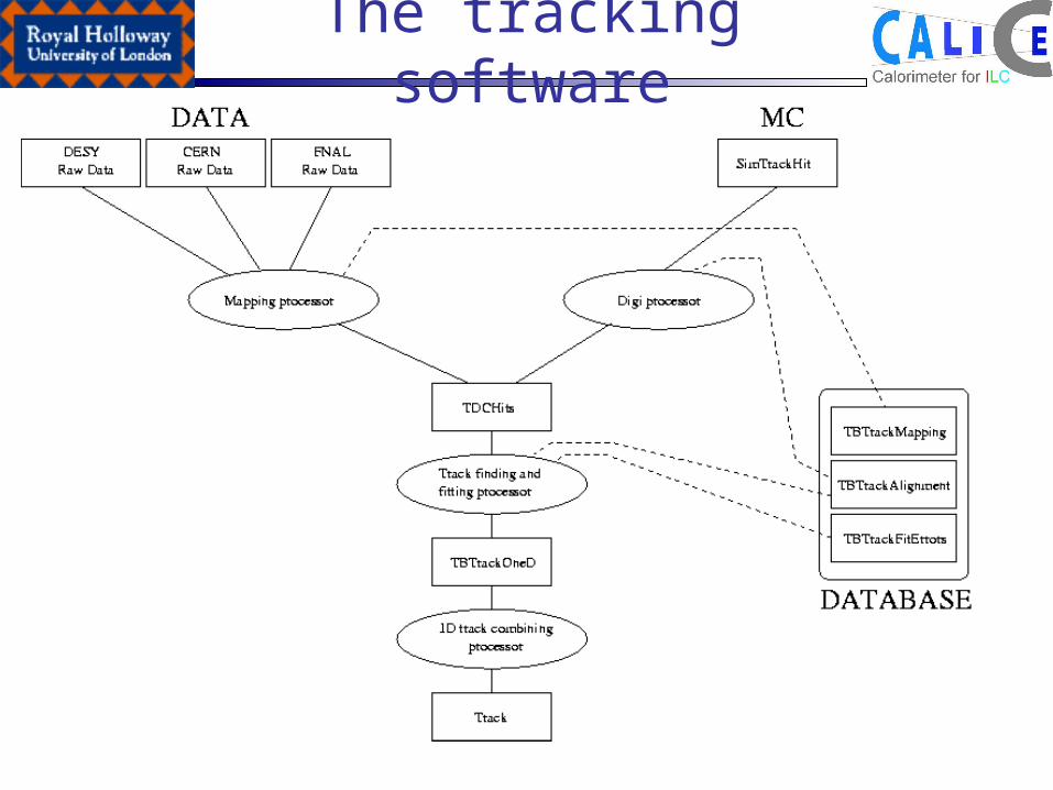
The tracking software

Drift velocity

• Several suggestion, no definitive answer.– Scatter plot– Ratio– Sum of consecutive chambers– Recursive methods– …

• The fact is we lack of external constraint. Some approximations are needed.

Results• First method abandoned

– fit a 2D Gauss and take the axis.

• Second method (X only)

• Third method, v1=v2 and v3=v4 (Y too)

Run Energy DC1 DC2 DC3 DC4

230097 3 0,0305 0,0284 0,0346 0,303

230098 1 0,031 0,0282 0,0386 0,0292

230099 2 0,0305 0,0284 0,035 0,0303

230100 4 0,0305 0,0282 0,0345 0,0302

230101 6 0,0303 0,0282 0,0342 0,0301230104 5 0,0301 0,0278 0,034 0,0299

230255 1,5 0,0299 0,0278 0,0339 0,0294

DC1-2 X 0,0296

DC1-2 Y 0,0303

DC3-4 X 0,0327

DC3-4 Y 0,0273

DC1-2 average = 0.0300

DC3-4 average = 0.0300

Track reconstruction• Error matrix calculated from MC events to evaluate the

multiple scattering, – intrinsic error is set to 0.4 mm for the moment

• Try assuming layer 0 and 3 have the same drift velocity– Start assuming drift velocity of 0.03mm/ns in each

• Interpolate inwards to determine constants of layers 1 and 2– Use full fit and shift offsets and drift velocities to get best

probability values– Effectively gives relative drift velocities to average of layer 0 and 3

• 1D Track can extrapolate the point at any Z– Error is propagated using the error matrix from MC

Results after alignment

• ~40% of events have no track• How much is due to noisy beam conditions at DESY?

• Need to compare with ECAL energy next

• ~20% of tracks have four hits• For efficiency see later

Intrinsic resolution• It is possible to evaluate the intrinsic resolution

constraining the Chi probability to be flat.

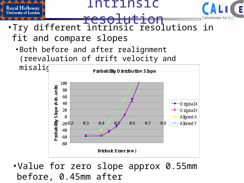
Intrinsic resolution• Try different intrinsic resolutions in fit and compare slopes• Both before and after realignment (reevaluation of drift velocity

and misalignment)

Probability Distribution Slope

-80

-60

-40

-20

0

20

40

60

80

100

0.2 0.3 0.4 0.5 0.6 0.7 0.8

Intrinsic Error (mm)

Pro

bab

ility

Slo

pe

(Arb

. un

its)

Original X

Original Y

Aligned X

Aligned Y

• Value for zero slope approx 0.55mm before, 0.45mm after

Intrinsic resolution (2)

• It is possible to evaluate the intrinsic resolution plotting the errors as a function of the energy.– The errors are evaluated using the formula

– With S defined as

– 2 cannot be used since nd is 2

1

modeˆ

dn

S

n

iii xfyS

1

2;

2

modeˆ

2

dn

S

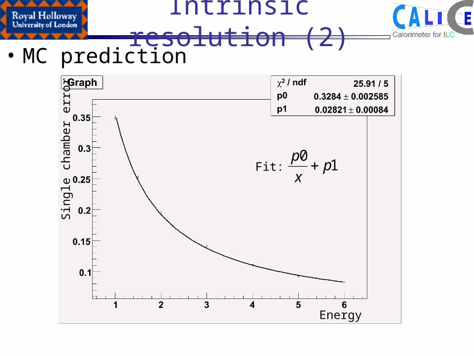
Intrinsic resolution (2)• MC prediction

Sin

gle

cham

ber

erro

r

Energy

Fit: 10

px

p

Intrinsic resolution(2)• Data

Sin

gle

cham

ber

erro

r

Energy

Fit: 10

px

p

Intrinsic resolution(2)• Increasing the errors

Sin

gle

cham

ber

erro

r

Energy

Fit: 10

px

p

Efficiency• Efficiencies have been evaluated last year

before the test beams, this is the result

Efficiency• All chambers have ~75-85% efficiency, this

means all wire have an efficiency ~90%– Chamber #3 that has 60% efficiency due to the Y

wire that is only ~65% efficient

• This result can be compared with the “effective efficiency” from the number of successfully reconstructed tracks

• Giving an efficiency of 70% for each wire

%20_#

_#4 eventstotal

tracksedrecontruct

MC-Data comparisonData MC

Layer 3 missing

All layers

Layer 0 missing

Layer 1 missing

Layer 2 missing

Conclusion• Software structure is defined, minor issue to be

decided. • MC simulation and digitization is available• Several method to evaluate drift velocity and

other constants– All are in good agreement

• More studies are undergoing to improve these values

• Tracking is almost ready, – this week last test will be performed to have the

tracking installed and debugged on Roman machine

Backup slides

XECAL vs tDC

(36-XECAL)/tDC

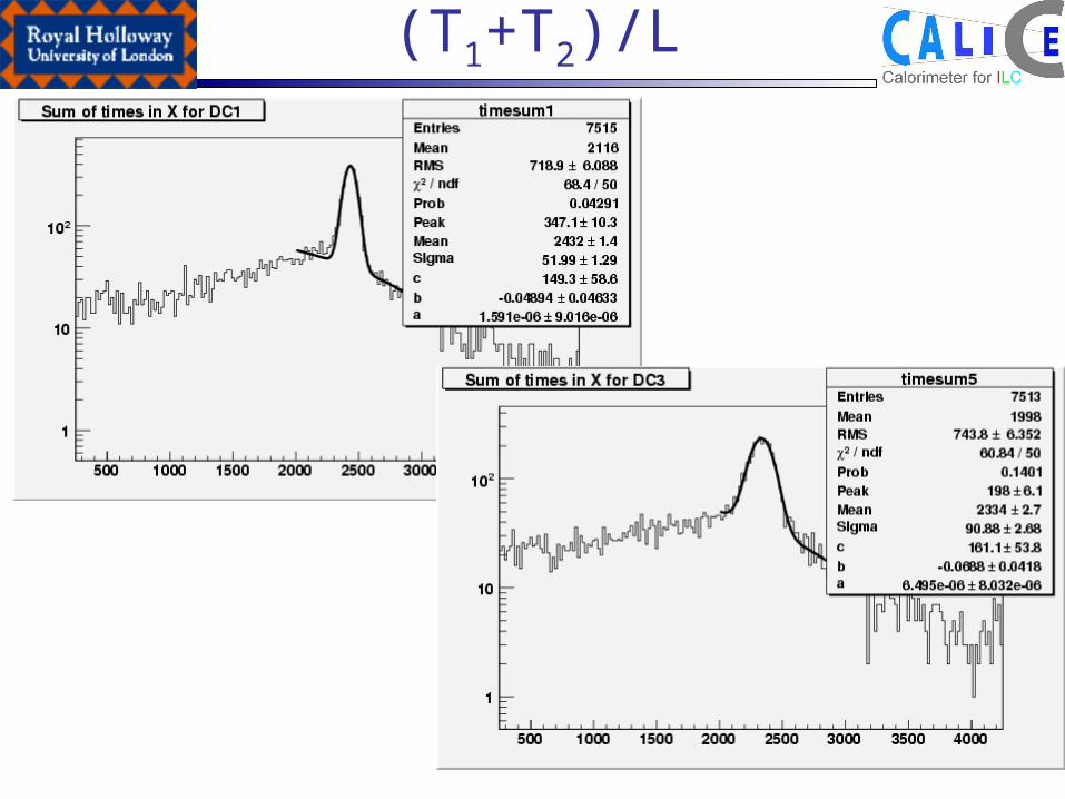
(T1+T2)/L

Drift velocity

DCECALECAL

DCECALECAL

ECALECAL

ECALECAL

DC

DC

OffOfftvX

OffOfftvX

OfftvX

OfftvX

OffLtvtv

Ltvtv

OffLtvtv

Ltvtv

44

33

22

11

4411

4433

3322

2211

ECal

DC1 DC2

DC3 DC4t1

t2

t3

t4

• All quantity have to be considered averaged

• Offset between DC1-DC2 and DC3-DC4 is 0.2mm, negligible on first approximation

• Y should be easier because of the better alignment:– OffYDC should be very small

Distributions