Statistical analysis of RTT variability in GPRSand UMTS networks

Jorma Kilpi∗ and Pasi Lassila∗∗

∗VTT Information Technology, P.O.Box 12022,FIN 02044 VTT, Finland.

∗∗Helsinki University of Technology, P.O. Box 3000,FIN 02015 HUT, Finland.

Email: Jorma.Kilpi@vtt.fi, Pasi.Lassila@hut.fi

November 18, 2005

Abstract

Abstract: We study the data from a passive traffic measurement representing a30 hour IP traffic trace from a Finnish operator’s GPRS/UMTS network. Of specificinterest is the variability of the Round Trip Times (RTTs) of the TCP flows in the net-work. The RTTs are analysed at both micro- and macroscopic level. The microscopiclevel involves detailed analysis of individual flows and we are able to infer variousissues affecting the RTT process of a particular flow, such as changes in the rate of theradio channel and the impact of simultaneous TCP flows at the mobile device. Also,Lomb periodograms are used to detect periodic behavior in the applications. In themacroscopic analysis we search for dominating RTT values first by Energy FunctionPlots and then by exploring spikes of empirical PDFs of aggrgate RTTs. Comparisonof empirical CDFs show significant shift in quantiles after considerable traffic increasewhich is found to be due to bandwidth sharing at individual mobile devices. Finally,we investigate further the impact of bandwidth sharing at the mobile device and showhow the increased amount of simultaneous TCP connections seriously affects the RTTsobserved by a given flow, both in GPRS and in UMTS.

1

1 Introduction

Traffic measurements are an important means when assessing the performance of real net-works. Using measurements one obtains direct evidence of the performance and, by ex-amining the measured data more closely, it is also possible to detect bottlenecks and/oranomalous behavior in the networks. Technology development is presently especially rapidin the field of wireless data networks. Hence, measurements in such networks, for exampleGPRS networks or newly deployed UMTS networks, are critical and are needed to under-stand the issues affecting the performance of TCP/IP traffic in such networks.

A measurement from a real operational network is always difficult, both technically andlegally. Technically, one major methodological issue is whether the measurement pro-cess/method is active or passive. An active measurement process allows one to carefullydesign the measurement such that the phenomenon of interest can be examined very accu-rately. However, one major drawback of the approach is that it is intrusive in the sense thatthe extra traffic caused by the measurement may impact the results. Thus, there is alwaysa fundamental question, whether a tailored active measurement is actually representative ofthe real network traffic. Passive measurements, on the other hand, refer to a measurementwhere one simply measures (captures) the real network traffic without injecting any extratraffic, and the method is hence by nature non-intrusive. Arranging such measurementsis usually more difficult, requiring sophisticated measurement equipment and negotiationswith network operators. The benefits are that there is no doubt about the representative-ness of the data and one can try to find out whether some phenomenon exists at a frequencythat is statistically relevant.

In this paper we study the data from a passive non-intrusive traffic capture measurementrepresenting a 30 hour IP traffic trace measured from one GGSN element of a GPRS/UMTSnetwork in a major Finnish network operator’s production network. TCP is the most oftenused transport protocol in IP networks and the objective of the measurement is to analyzecertain properties of TCP flows where one end point of the flow is in the GPRS/UMTSnetwork and the other in the public Internet. Due to the structure of the GPRS/UMTSnetwork, measuring at the GGSN node gives the possibility to observe all TCP flows whichtraverse the considered GGSN node in the network. Of specific interest in the data is thevariability of the Round Trip Times (RTTs) observed by the TCP flows. Large variability ofthe RTTs may cause problems for example to TCP’s retransmission mechanism in the formof spurious timeouts (see, e.g. [10], [8], [7], [18], [12] and [16]). As opposed to the activemeasurement approach used in [10] and [8], we have a passive measurement of the actualnetwork traffic (comments on other passive measurement studies are provided Section I.A).

The objective of this study is to analyse thoroughly the statistical properties of the RTTprocess as observed by the TCP flows. To this end, we perform a detailed analysis of theRTTs of selected individual flows (microscopic analysis) and the RTTs of the aggregatetraffic (macroscopic analysis). Furthermore, as the measurement data contains TCP flowsboth from GPRS users and UMTS users, we are able to compare the properties of the RTTprocess for both technologies.

2

Briefly, our measurement analysis methodology and our main observations are the follow-ing. First the quality of the time stamps on the captured IP packets is validated and wedemonstrate that the measurement equipment or the setup itself has not impaired the data.The summary data is obtained by using a program called tstat [1], which gives informationabout TCP connections/flows. We use the summary data to get information about the rawdata and, with the help of summary data, select TCP flows that seem to be interesting forour microscopic-level analysis. The idea is to select long flows, so that it is possible to detectqualitative changes in the RTT process over a relatively long period of time. In the micro-scopic analysis, we are able to address issues such as changes in the sending rate of a TCPflow and the impact of simultaneous TCP connections. Furthermore, by using the Lombperiodogram (see Section I.A), one can identify if transmission patterns behind the RTTprocess are periodical. In the macroscopic analysis we search for dominating RTT valuesfirst by Energy Function Plots, based on the Haar wavelet, and then by exploring spikes ofempirical PDFs of aggregate RTTs. Comparison of empirical CDFs show significant shift inquantiles after considerable traffic increase which is found to be due to bandwidth sharingat individual mobile devices. Additionally, we show how the change of tariff has a clearimpact on the way that the users behave - during the flat rate period users seem to openmore simultaneous TCP connections than during the day time indicating increased web ac-tivity during flat rate charging. Finally, the importance of the amount of simultaneous TCPconnections a mobile has, both in our micro- and macroscopic analysis, on the maximumRTTs a flow observes, lead us to believe that it is actually the presence of competition forbandwidth at the mobile device that is responsible for the very high values of RTTs thatsome flows observe. This issue is investigated in detail and, indeed, we show that increaseddegree of bandwidth sharing results in larger (even excessive) maximum RTTs.

The paper is organized as follows. In Section II, the measurement setup and the equipmentis discussed, and the quality of the time stamps is verified. The microscopic analysis ofcertain flows, both for GPRS and UMTS, are presented in Section III. The macroscopicanalysis of the RTTs is in Section IV, while Section V analyses the impact of bandwidthsharing at the mobile device on the RTTs. Conclusions are provided in Section VI.

1.1 Related Work

Many measurements of RTT have been recently made both in mobile/wireless and wiredaccess networks. For example, a similar GPRS measurement made in Austria is reported in[17] and a study of spurious timeout events in TCP/GPRS is reported in [18]. In addition tothis, a similar GPRS measurement made from seven different European and Asian countriesis reported in [4]. Our study complements these studies by representing a GPRS trafficmeasurement made in Finland, and its statistical analysis.

Our emphasis has also been on investigating existing statistical tools that could be used inanalysing RTTs. The paper [3] reports a similar, but non-mobile, study of RTT variationbased on a very large data set collected at the ISP link of the University of North Carolineat Chapel Hill. Their data contained also some, but unknown, proportion of wireless access

3

connections. They defined a connection experiencing ’high variability’ if the interquartilerange (IQR), i.e. the difference between 75th and 25th percentiles of an RTT sample of theconnection, was strictly larger than the difference between the median (50th percentile) andthe minimum,

IQR > Median RTT− Minimum RTT. (1)

Minimum RTT is used as the estimate of the non-random component of RTT. In the datathey had the condition (1) accounted for over 50% of the connections. Use of percentilesmakes the statistic

IQR/( Median RTT− Minimum RTT), (2)

briefly IQR/(Md-Min), very robust but requires the number of the RTT sample values perflow to be large enough. In [3] the authors required at least 10 valid RTT samples per flow.

The paper [9] used wavelets, more precisely energy function plots (EFPs), applied to the’signal‘ of aggregate traffic, both measured and simulated, in order to detect network per-formance problems indicated by significant changes in the dominating RTT values.

In [15] a statistical tool called the Lomb periodogram (LP) [11] was used in a very interestingexperimental set-up where it was able to find timing properties of a data flow from the tracethat contained only traffic of another data flow. This latter flow had only shared someresources with the former flow.

We have also tested and used (2), LPs and EFPs as a methodological starting points in ouranalysis.

2 Measurement environment and equipment

2.1 The monitoring port of a GGSN

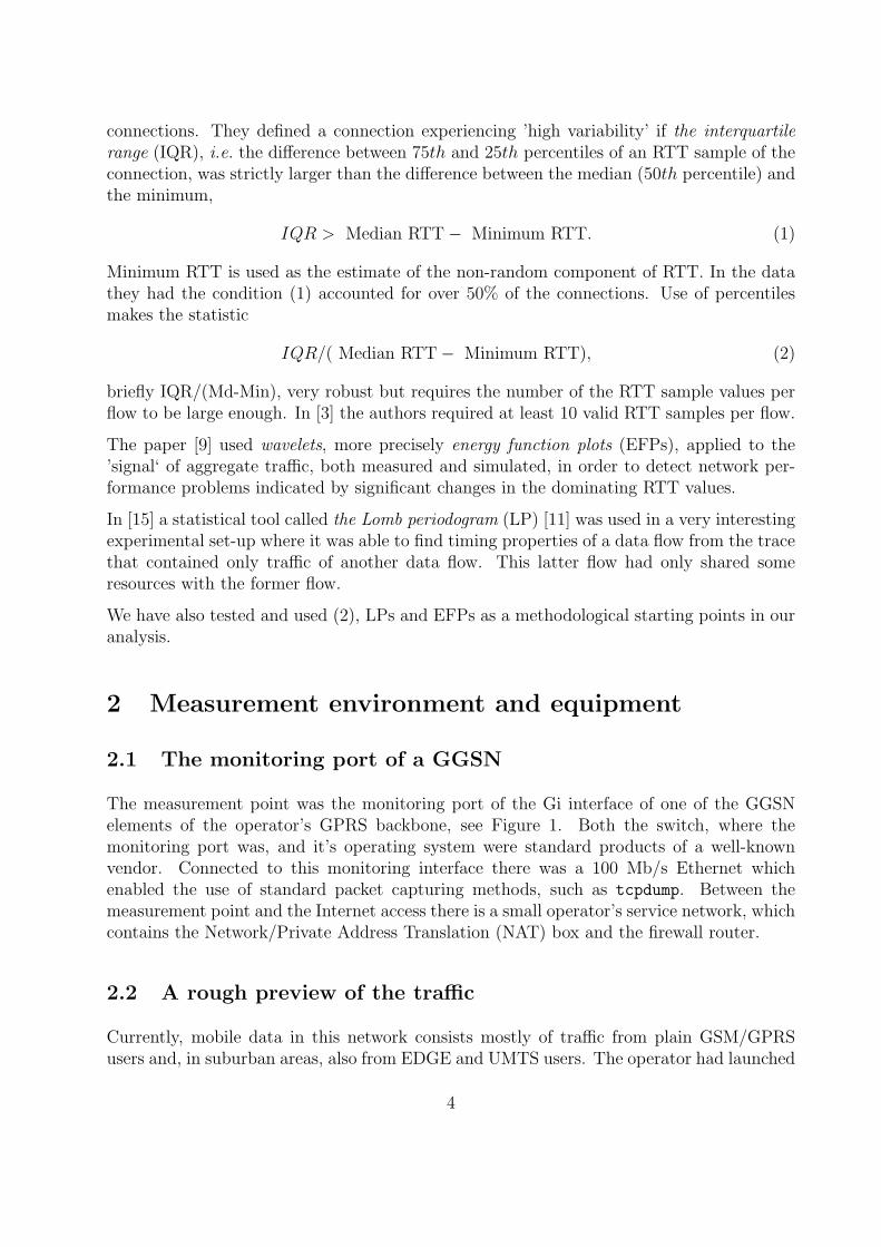
The measurement point was the monitoring port of the Gi interface of one of the GGSNelements of the operator’s GPRS backbone, see Figure 1. Both the switch, where themonitoring port was, and it’s operating system were standard products of a well-knownvendor. Connected to this monitoring interface there was a 100 Mb/s Ethernet whichenabled the use of standard packet capturing methods, such as tcpdump. Between themeasurement point and the Internet access there is a small operator’s service network, whichcontains the Network/Private Address Translation (NAT) box and the firewall router.

2.2 A rough preview of the traffic

Currently, mobile data in this network consists mostly of traffic from plain GSM/GPRSusers and, in suburban areas, also from EDGE and UMTS users. The operator had launched

4

GPRS network

GGSN FirewallFirewall

Service network

PublicInternetPublicInternet

mobile hostmobile host external hostexternal host

Gn Gi

datadata

ACKsACKs

semi-RTT

Figure 1: The measurement scenario.

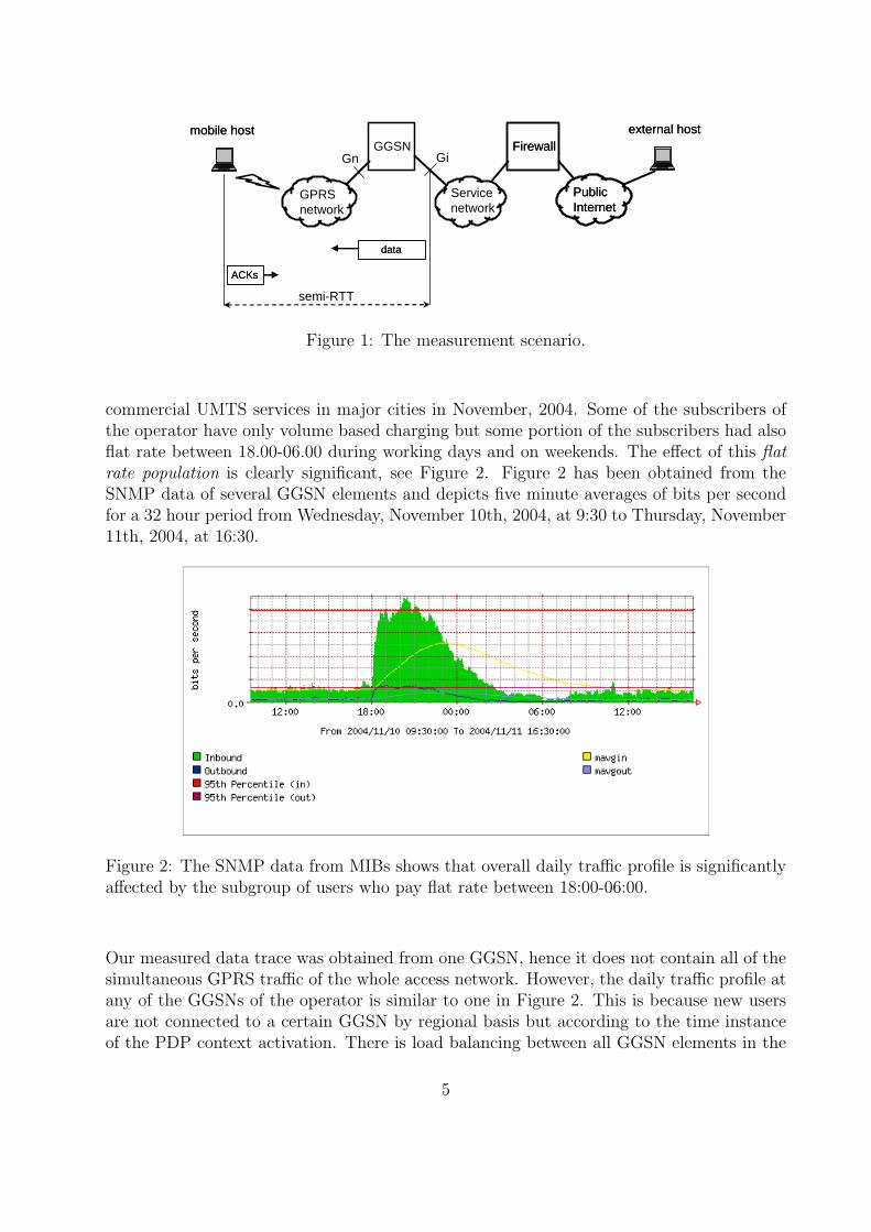
commercial UMTS services in major cities in November, 2004. Some of the subscribers ofthe operator have only volume based charging but some portion of the subscribers had alsoflat rate between 18.00-06.00 during working days and on weekends. The effect of this flatrate population is clearly significant, see Figure 2. Figure 2 has been obtained from theSNMP data of several GGSN elements and depicts five minute averages of bits per secondfor a 32 hour period from Wednesday, November 10th, 2004, at 9:30 to Thursday, November11th, 2004, at 16:30.

Figure 2: The SNMP data from MIBs shows that overall daily traffic profile is significantlyaffected by the subgroup of users who pay flat rate between 18:00-06:00.

Our measured data trace was obtained from one GGSN, hence it does not contain all of thesimultaneous GPRS traffic of the whole access network. However, the daily traffic profile atany of the GGSNs of the operator is similar to one in Figure 2. This is because new usersare not connected to a certain GGSN by regional basis but according to the time instanceof the PDP context activation. There is load balancing between all GGSN elements in the

5

sense that the fraction of users connected to one GGSN element is, in the long run, relativeto the total number of GGSNs.

2.3 Technical requirements

Capturing of TCP traffic at the above described measurement point for a long enough time,say 24 hours, should give a representative sample of TCP connections. The remainingtechnical requirements are the quality of time stamps, as all RTT statistics are based onthem, and capturing of every single packet.

Minimum values of IP packet transfer delay is hundreds of milliseconds for GPRS/GSM andtens of milliseconds for UMTS. Thus, millisecond accuracy would be sufficient. However,to guarantee any accuracy is not easy to achieve using Linux, tcpdump and an ordinaryoff-the-shelf PC.

The time stamps are called precise if their random variability is small. The time stampsare called accurate if both their variability and bias are small. The time stamp that thetcpdump program gives is associated to the end of the corresponding packet, see [14]. Thebias is thus considered as relative to the ’time instance of the last bit of the Ethernet framethat carried the corresponding packet‘.

Since we needed to capture and save all the traffic in a disc, while the quality of time stampsmust simultaneously be kept high, some optimisation of the measurement equipment, a2.4MHz computer with Linux operating system and a 160 GB IDE hard disk, had to bemade. The computer has the 10/100 Ethernet card integrated in the mother board. Weused Debian Linux kernel 2.6.8 compiled with the preemptible kernel option. The harddisk was optimised using options that enabled Ultra Direct Memory Access (UDMA) mode,32 bit words and simultaneous writing onto 16 sectors with one CPU command. The filesystem, ext3, was optimised using synchronous writing and minimising journaling overhead.Following the advice from [5] the measurement was performed in the single-user mode withNTP1 disabled.

Due to SNMP information, like in Figure 2, and a preliminary test measurement we had quiteprecise knowledge about the traffic load at the measurement point. The packet capturingand time stamping features of the optimised Linux computer, described above, were testedbeforehand using Ethernet 10/100BASE-T and GbE interfaces of the Adtech AX/4000traffic generator of Spirent Communications and with a load that was two and three timesmore than the observed maximum load at the actual measurement interface was. Even witha threefold load the packet capturing, time stamping and saving still worked perfectly. Infact, the maximum bias with the traffic generator test with threefold load was less than ourtarget accuracy ±50µs. This is about the best that can be achieved using ordinary NICs,since they do not generate CPU interrupts more often.

The data trace we use in this paper was measured from Wednesday, November 10th, 2004,

1NTP was implemented only to see the drift of the computer’s clock, −1.21± 0.5p.p.m.

6

at 10:30 to Thursday, November 11th, 2004, at 16:30. The tcpdump program reported 0dropped packets, and the Ethernet card’s driver did not report any dropped or anomalousEthernet frames.

One way to check the accuracy of time stamps is to plot the packet inter-arrival timeti+1 − ti against the packet’s size Bi+1, remembering that the time stamp of tcpdump mustbe associated at the end of the packet’s Ethernet frame. This is shown in Figure 3 below:with accurate time stamps we should be able to see the 100 Mb/s Ethernet’s transfer ratewhich, knowing the framing structure of the Ethernet, can easily be calculated theoreticallyassuming packets arrive back-to-back. The calculated dashed line is also shown in Figure3. The packets’ true spacings cannot be too close to each other. If they are too close toeach other, it is a sign of buffering at the measurement equipment before the time stampis attached to packets. Figure 3 represents a piece from the busy hour period and pointsbelow the dashed line show that some buffering before time stamping had occured. The biasfor large packets is the vertical distance between a point and the dashed line. As can be

0 200 400 600 800 100012001400

IP Packet Size (B)

0

20

40

60

80

100

120

IAT

(mic

rose

cond

s)

ti+1 -ti vs. Bi+1

Figure 3: Packet inter-arrival time against the packet size.

seen, the granularity of time stamps is not sufficient to distinguish correctly small packetsthat arrive back-to-back. Their inter-arrival time may be too small but is within the ±50µsbound. This is not a problem in our study.

Another way to view the time stamps ti is to make plots of (ti, ti mod h), with a suitablychosen h, for example, h = 1ms or h = 1s. These type of plots show if there are significantgaps in the time stamps. Such gaps do not show up in plots like 3. In summary, we areconfident that the accuracy of time stamps is very good with bias less than the targetaccuracy ±50µs.

7

2.4 Re-building of TCP connections

Before anonymization the packet level data was given as input to the tstat-program, [1]. Weused a test version 1.0beta15 of tstat. When processing the packet data, tstat maintainsa list of all TCP connections and, when analysing the next TCP/IP packet, rebuilds thecorresponding TCP connection status. If all the phases of a TCP connection are properlyobserved, the connection statistics are calculated and written into a file as one record whichcontains 92 different attributes. Otherwise a record is written into another file. The recordin the file of incompletely observed connections still contains valid information about IP-addresses, TCP ports and the number of SYN packets. It was used to detect anomalies, likeport scanning, in the data. However, all our analysis in this paper is based only on thoseconnections that tstat recorded as completely observed in the sense that opening and closingwere correctly observed, as described above. Since the packet loss in the measurement waszero, these completely observed connections are complete also in the sense that every singlepacket of them is also observed.

2.5 Semi-RTT

Semi-RTT refers to the difference of the time stamps of a (downstream) TCP/IP packetcarrying some data payload and of the corresponding ACK packet, see again Figure 1. Sincethese time stamps are measured at the Gi interface the semi-RTT is not the same as anend-to-end RTT but, like in [17] we call it simply as RTT.

For each completely observed TCP connection tstat provides some (semi-) RTT informa-tion automatically: minimum, maximum, mean, standard deviation and the number of timesa data segment and the corresponding ACK has been observed. This latter value, denotedhere by RTT count, is directly relative to the size of the flow. Moreover, to avoid that out-of-sequence and duplicate segments or ACKs provide unreliable measurements that affectthe RTT measurement itself, only samples referring to in-sequence segments are considered.This RTT information is given in both down- and upstream directions.

However, since the built-in RTT statistics of tstat were not enough for this study the codeof the tstat-program was modified in a way that we got out every valid RTT value of everycompletely observed connection and enough information to associate each individual RTTvalue with the connection that it belongs to.

3 Classification methodology

The arrival time of a completely observed TCP connection is determined by the time stampof the handshaking SYN packet sent by the client. Downloadings are first classified accordingto TCP connection arrival times into 5 distinct groups as explained in Table 1 below. Recallthat the flat rate population is a subset of subscribers of the operator.

8

Sample TCP Connection Flat RateNumber Arrival Time Population

Present?1 10:30-18:00 No2 18:00-21:00 Yes3 21:00-24:00 Yes4 00:00-06:00 Yes5 06:00-16:30 No

Table 1: Division into subsamples according to TCP connection arrival time.

Samples 1 and 5 were statistically similar to each other, also samples 2 and 3 were similar toeach other. Thus, to analyse the impact of tariff change, we compare only sample 1 versus2. Analysis of the sample 4 is not contained in this paper.

3.1 RTT Count as a measure of a size of the downstream flow ofa TCP connection

Further division of data is based on the concept of the (downstream) RTT Count which isthe number of valid RTT samples per downloading part of a TCP connection. Since theeffect of the packet size is significant, the RTT value obtained from the three-way handshakeis not included in our analysis.

RTT Count is a measure of the size of the downstream flow of a TCP connection. It isrelative both to the duration of a downloading and to the amount of (unique) bytes thatare downloaded, see Figures 4 and 5. The same concept was essentially used in [17] as ameasure of size.

The concept of Unique Bytes is defined as the amount of bytes correctly acknowledged, notincluding retransmitted, duplicated or in some other sense anomalious bytes. This is alsoone of the statistics that tstat provides.

Figure 4 shows RTT Count compared against downloaded Unique Bytes (MB). The linesshow how the size in bytes would develope if each increment in RTT Count would be dueto acknowledging only a single segment of size 536 or 1460 bytes, respectively.

For a downloading flow the RTT count increases approximately linearly with Unique Bytes.If the corresponding TCP connection downloads data in small segments the amount ofdownloaded Unique Bytes can be small with RTT count large. If, for example, a connectiongenerates other TCP connections for data transfer, its duration can be very long even if thedownstream RTT count is rather small as shown in Figure 5.

9

0 10 20 30 40 50 60Unique Bytes (MB)

0

10000

20000

30000

40000

RT

TC

ou

nt

RTT Count vs. Unique Bytes

536

1460

Figure 4: RTT Count against downloaded Unique Bytes (MB).

0 3 6 9 12 15 18 21 24Duration (h)

0

10000

20000

30000

40000

RT

TC

ou

nt

RTT Count vs. Connection Duration

Figure 5: RTT Count against TCP connection duration.

10

3.2 Division of downstream flows according to RTT count

We are not very interested in the duration of a flow. The word ’long’ is used here to meanlong in the sense that the RTT Count is large. More detailed statistical analysis is made onlyfor those flows that were longer than at least 6 RTT counts, with RTT from the handshakingexluded. Figure 6 shows that using the value 6 as a discriminating value divides each sample

101 102 103 104 105

RTT Count

1

10-1

10-2

10-3

10-4

10-5

CC

DF

6

0.25

Division of Flows

10:30-18:00

18:00-21:00

Figure 6: The condition RTT Count ≥ 6 includes ≈ 25% of the downstream flows (andexcludes ≈ 75%).

into approximately 25% of long flows and 75% of short flows. The tariff change does nothave any effect on that. Flows shorter than 6 RTT counts were analysed only by studyingthe distribution of the range of RTT. This is presented in section 5.1.

We also studied the number of applications with relatively long flows in terms of RTT Count.Table 2 shows, according to the server port number, the 12 most frequent applicationswhich had RTT Count > 1 000. In total, there were 145 different applications that hadRTT Count > 1 000.

4 Microscopic analysis of long TCP flows

A rather complete analysis of a number of individual long flows were primarily made in orderto understand how the radio interface affects the RTTs. There were also other questions,such as does the considerable increase of traffic due to the tariff change show up somehowin RTTs? The question that concerns the operator is that does the flat rate populationdisturb ordinary subscribers who pay per volume? (The flat rate population is not directlyrelated to the operator but through a household appliance selling company.) In general, theidea is to find out what can be deduced from changes in the RTT during a flow.

Some specifically chosen examples are presented here first in order to give a reader a flavour

11

Port Application Explanation Frequency119 nntp 9

1863 msnp 9443 HTTPS Web 11

4662 eDonkey P2P 111214 kazaA P2P 13411 rmt 13

43594 runescape Game 228080 HTTP-alt Web 24

10000 ndmp 25110 pop3 Mail 30

6699 napster? P2P 4680 HTTP Web 439

Table 2: The 12 most frequent applications that had RTT Count > 1 000.

of what is behind a macroscopic level analysis that will be presented later. Example flowswere chosen because the time series

{(ti, RTT (ti)) | i = 1, . . . , RTT Count} (3)

had some distinctive features. In (3) the ti is the time stamp of an ACK packet and RTT (ti)is the RTT value calculated from the ACK packet.

4.1 Individual TCP flows in GSM/GPRS

Some key properties of the three individual TCP/GPRS (and two TCP/UMTS) downstreamflow examples are collected to Table 3 below. They all used the SACK option. Unique Bytesis given in MB.

Property Flow1 2 3 4 5

SACKs 2795 22 797 165 74RTT Count 32 479 7 427 16 078 6351 13961Unique Bytes 32.5 9.9 22.6 5.6 22.1IQR/(Md-Min) 0.79 0.11 0.29 0.84 0.36

Table 3: Three TCP/GPRS and two TCP/UMTS downstream flows.

12

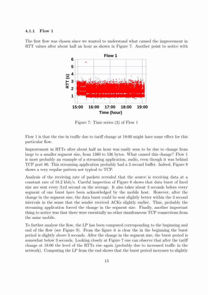
4.1.1 Flow 1

The first flow was chosen since we wanted to understand what caused the improvement inRTT values after about half an hour as shown in Figure 7. Another point to notice with

15:00 16:00 17:00 18:00 19:00Time (hour)

1

2

3

4

5

6

RT

T(s

)

Flow 1

Figure 7: Time series (3) of Flow 1

Flow 1 is that the rise in traffic due to tariff change at 18:00 might have some effect for thisparticular flow.

Improvement in RTTs after about half an hour was easily seen to be due to change fromlarge to a smaller segment size, from 1380 to 536 bytes. What caused this change? Flow 1is most probably an example of a streaming application, audio, even though it was behindTCP port 80. This streaming application probably had a 3 second buffer. Indeed, Figure 8shows a very reqular pattern not typical to TCP.

Analysis of the receiving rate of packets revealed that the source is receiving data at aconstant rate of 18.2 kbit/s. Careful inspection of Figure 8 shows that data burst of fixedsize are sent every 3:rd second on the average. It also takes about 3 seconds before everysegment of one burst have been acknowledged by the mobile host. However, after thechange in the segment size, the data burst could be sent slightly better within the 3 secondintervals in the sense that the sender received ACKs slightly earlier. Thus, probably thestreaming application forced the change in the segment size. Finally, another importantthing to notice was that there were essentially no other simultaneous TCP connections fromthe same mobile.

To further analyse the flow, the LP has been computed corresponding to the beginning andend of the flow (see Figure 9). From the figure it is clear the in the beginning the burstperiod is slightly above 3 seconds. After the change in the segment size, the burst period issomewhat below 3 seconds. Looking closely at Figure 7 one can observe that after the tariffchange at 18:00 the level of the RTTs rise again (probably due to increased traffic in thenetwork). Computing the LP from the end shows that the burst period increases to slightly

13

180 190 200 210 220 230 240Time (Seconds from the Flow Arrival)

1.251.5

1.752

2.252.5

2.753

RT

T(s

)

Flow 1 Zoomed

Figure 8: Time series of Flow 1 zoomed.

2.25 2.5 2.75 3 3.25 3.5 3.75 4Time Period (s)

0

20

40

60

80

100

120

Spec

tral

Pow

er

Lomb Periodogram of Flow 1

Begin

Middle

End

Figure 9: The Lomb Periodogram calculated for Flow 1.

14

above 3 seconds again.

4.1.2 Flow 2

The Figure 10 shows the remarkable property of flow 2, namely that RTTs at level 5.0-7.5seconds seems to be normal for this connection. Also, the minimum is less than 1 second,

17:30 17:45Time (hour)

2.55

7.510

12.515

17.520

RT

T(s

)Flow 2

Figure 10: Time series of Flow 2

hence a better level could be possible.

Unlike for Flow 1, within the limits 5.0-7.5s use of LP showed that there was no regularperiodic structure for Flow 2. Moreover, as Figure 11 indicates, there was a change inthe downlink capacity from 40.2 kb/s to 26.8 kb/s, which corresponds to a loss of onePDCHs in the downlink when CS-2 is the channel coding scheme. Finally, as Figure 12shows, the change in the link capacity for Flow 2 was due to self-congestion caused by othersimultaneous TCP connections from the same mobile host. Large RTT values were probablydue to a low terminal capacity.

4.1.3 Flow 3

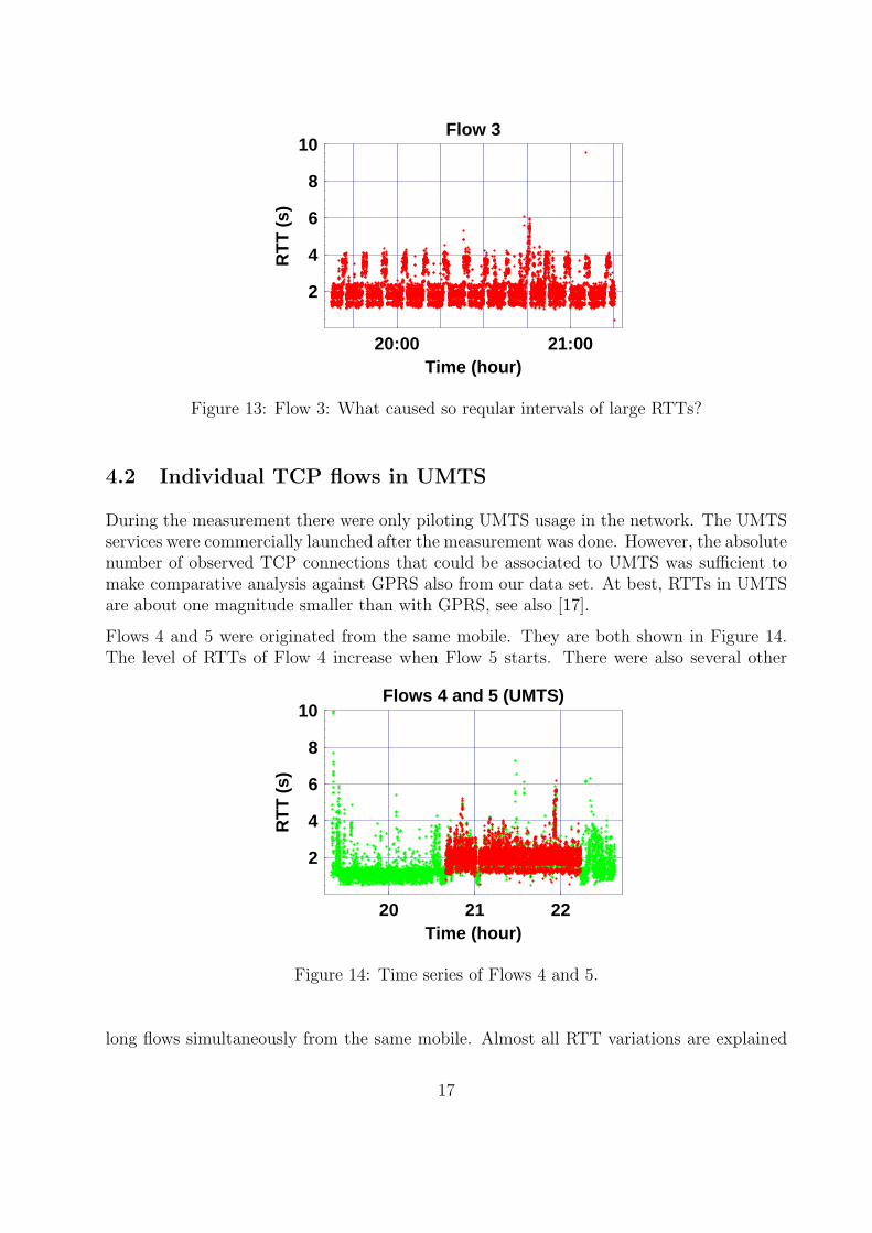
Again, use of LP showed no regular periodicities. However, Flow 3 had some peculiar reqularintervals of bad RTTs. In this case the self-congestion is also an explanation since the userwas simultaneously running an application (MSNP) which caused, each time with a newflow in port 80, regularly within approximately 8 minute intervals a downloading of exactly265.3 kB file. These downloadings occur exactly at the bad intervals visible in Figure 13.

15

0 5 10 15 20 25 30 35Time from the First Segment (min)

0

2

4

6

8

10

Vo

lum

e(M

B)

Flow 2

End: 26.8 kb/s

Begin: 40.2 kb/s

Figure 11: Change in the downlink capasity for Flow 2.

17:15 17:30 17:45 18:00 18:15Flow End Points

0

20

40

60

80

100

i:th

Flo

w

Simultaneous flows with Flow 2

Flow 2

Figure 12: Change in link capasity for Flow 2 is due to self congestion.

16

20:00 21:00Time (hour)

2

4

6

8

10

RT

T(s

)

Flow 3

Figure 13: Flow 3: What caused so reqular intervals of large RTTs?

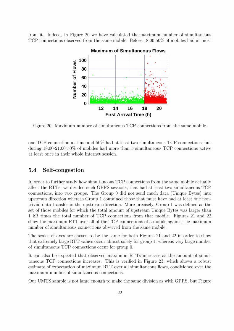
4.2 Individual TCP flows in UMTS

During the measurement there were only piloting UMTS usage in the network. The UMTSservices were commercially launched after the measurement was done. However, the absolutenumber of observed TCP connections that could be associated to UMTS was sufficient tomake comparative analysis against GPRS also from our data set. At best, RTTs in UMTSare about one magnitude smaller than with GPRS, see also [17].

Flows 4 and 5 were originated from the same mobile. They are both shown in Figure 14.The level of RTTs of Flow 4 increase when Flow 5 starts. There were also several other

20 21 22Time (hour)

2

4

6

8

10

RT

T(s

)

Flows 4 and 5 (UMTS)

Figure 14: Time series of Flows 4 and 5.

long flows simultaneously from the same mobile. Almost all RTT variations are explained

17

by these other flows.

5 Properties of RTT at the macroscopic level

5.1 Short downstream flows

When the RTT Count is less than 6, with the handshaking RTT not included, it is not easyto make any kind of analysis about the RTT process (3). As already mentioned these shortflows consist of about 75% of TCP downstream flows, but only a fraction of all downstreamUnique Bytes. For the sake of completeness we also present some analysis of these shortflows.

The RTT range, difference of the maximum and the minimum RTT values per flow, seemsto be the best general statistic for short flows. We know that these extremal values arehighly non-robust but we trust the accuracy of our time stamps. Figure 15 shows the CDFsof RTT ranges of downstream flows of sample 1, when classified according to RTT Countwith values 3,4,5 and 6. It contains also the case RTT Count = 6 in order to make it overlapwith the analysis of long flows.

1 2 3 4 5RTT Range (s)

0

0.2

0.4

0.6

0.8

1

CD

F

Sample 1

RTT Count = 3

RTT Count = 4

RTT Count = 5

RTT Count = 6

Figure 15: The range of RTTs of short flows.

Figure 16 compares short flows of samples 1 and 2. For clarity, only RTT Counts 3 and 5are shown, others are similar. As can be seen, the ranges of the RTTs clearly increase.

5.2 The dominating RTT values

A superposition of many TCP connections can be assumed to produce local periodicitiesin the packet level aggregate traffic since the dynamics of an individual TCP connection

18

1 2 3 4 5RTT Range (s)

0

0.2

0.4

0.6

0.8

1

CD

F

Sample 2 vs. Sample 1

Sample 1

Sample 2

(RTT Counts 3 and 5)

Figure 16: Comparison ranges of RTTs of short flows.

depend on RTT. If there are dominant values of RTT, they should then be ’hidden‘ also inthe aggregate TCP traffic rate.

Figure 17 shows how the EFP, using the Haar wavelets, see [9, 6, 13, 2], looks for our data.It contains energy values of different scales of two packet level aggregate traffic sampleswhere the flat rate population is present and one sample, represented by the lowest curve,from the time period where the flat rate population is not present .

2 4 6 8 10 12j:th Scale

23456789

log 2

Ej

Energy Function Plot

Figure 17: Energy function plot.

Significant periodicities at the corresponding scale should show up in EFPs as ’dips’ down-wards. The 0th scale in Figure 17 contains packets per 10ms bins, the dip occurs in allcases in scales 6,7, 8 and 9 which corresponds to 0.64s, 1.28s, 2.56s and 5.12s bins. Thedominant RTT values, if they exist, can be expected to be found between half second and

19

five seconds.

In order to see more closely the values where the dips downwards starts and where thecurves start to rise up again we simply varied the initial bin sizes. We made this for sampleswhere the flat rate population is present and for samples where the flat rate population wasnot present. The differencies were found small.

We now turn back from the packet level data to the RTT data. From now on the word’aggregate‘ in this section means the set of all RTT samples without making any distinctionto what flows they belong. The long flows, with RTT Count at least 6, are not separatedfrom short flows either.

In order to compare dominating RTT values we calculated estimates of the PDFs simply asnormalised histograms. Normalised because we wanted to compare the positions of spikesin the histograms. The heights of the spikes are then only relative to to sample sizes, whichwere different. Sample 2 was about four times larger than Sample 1.

In GPRS, the Abis interface causes a granularity of 20 ms in the upstream traffic. Smallervariations are basically not due to radio interface. We wanted to capture the variations dueto radio interface but we were not so interested in the variations caused by the network.Hence we decided to use a bin size of 10 ms.

0 1 2 3 4 5 6 7 8 9 10RTT (s)

0

0.002

0.004

0.006

0.008

PD

F

1.3 4.3Positions of Spikes in PDFs

Sample 1

Sample 2

0.7 1.9

Figure 18: The positions of spikes do not differ much.

The long flows (25% of all) dominate the histograms: If the short flows (75% of all) were leftout, the histograms would still have the same shapes and spikes at the same positions. Onthe other hand, leaving out the longest flows of each sample does not change the histogramseither. The Sample 1 had spikes at positions 0.7, 1.3, 1.9 and 4.3 seconds, they are marked inFigure 18. The Sample 2 had also spikes at the same positions. Note that the positions of thespikes correspond to the typical transmission delays of a packet and its acknowledgementwhen the packet is sent directly without any buffering at SGSN where the buffer is permobile, after a queuing delay of one data packet, etc. This also implies, that the long flows

20

are not much affected by other traffic in the network. They are only constrained by theirown limited radio access link.

The prior information about lower tariff population, that some of them use mobile as analternative to dial-up connections in the regions where no broadband is available, suggeststhat typically they are far from base stations also, hence they may also often have heavierFEC property in their channel codings than the normal tariff population. Indeed, sample 2has clear spikes also in about 1 second and slightly less than 3 seconds in places where thesample 1 does not have so clear spikes.

The positions of spikes do not practically differ with different samples so histograms ofsamples 3 and 5 need not be shown here. Especially the traffic increase due to tariff changedoes not seem to have significant effect on positions of spikes. Only for the relative heightsof the spikes. This suggests that, in case of long flows, perhaps the lower tariff populationdoes not disturb normal tariff population significantly.

The Flow 2 in Figure 10 shows that minor spikes in the histogram of sample 1 near 6 secondsare still in the range of our interest.

5.3 Changes in quantiles

From the histogram based estimates of the PDFs we calculated also CDFs. Long flowsdominate also them. Figure 19 compares samples 1 and 2. Shift in the 0.25 and 0.5

0 1 2 3 4 5 6 7 8 9 10RTT (s)

0.05

0.25

0.5

0.75

0.95

CD

F

5.9 7.4

0

1

Change in Quantiles

Sample 1

Sample 2

Figure 19: Comparison of CCDFs.

quantiles is likely due to increased amount of long connections that are not close to basestations and thus use heavier channel coding scheme.

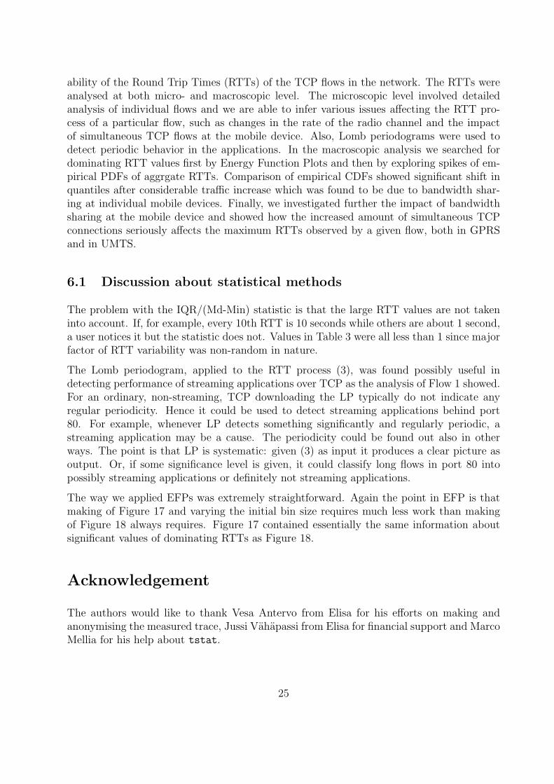
Significant increase of the 0.95 quantile, from 5.9s to 7.4s, is due to the increased amountof bandwidth sharing at individual mobile device due to simultaneous TCP connections

21

from it. Indeed, in Figure 20 we have calculated the maximum number of simultaneousTCP connections observed from the same mobile. Before 18:00 50% of mobiles had at most

12 14 16 18 20First Arrival Time (h)

0

20

40

60

80

100

Nu

mb

ero

fF

low

s

Maximum of Simultaneous Flows

Figure 20: Maximum number of simultaneous TCP connections from the same mobile.

one TCP connection at time and 50% had at least two simultaneous TCP connections, butduring 18:00-21:00 50% of mobiles had more than 5 simultaneous TCP connections activeat least once in their whole Internet session.

5.4 Self-congestion

In order to further study how simultaneous TCP connections from the same mobile actuallyaffect the RTTs, we divided such GPRS sessions, that had at least two simultaneous TCPconnections, into two groups. The Group 0 did not send much data (Unique Bytes) intoupstream direction whereas Group 1 contained those that must have had at least one non-trivial data transfer in the upstream direction. More precisely, Group 1 was defined as theset of those mobiles for which the total amount of upstream Unique Bytes was larger than1 kB times the total number of TCP connections from that mobile. Figures 21 and 22show the maximum RTT over all of the TCP connections of a mobile against the maximumnumber of simultaneous connections observed from the same mobile.

The scales of axes are chosen to be the same for both Figures 21 and 22 in order to showthat extremely large RTT values occur almost solely for group 1, whereas very large numberof simultaneous TCP connections occur for group 0.

It can also be expected that observed maximum RTTs increases as the amount of simul-taneous TCP connections increases. This is verified in Figure 23, which shows a robustestimate of expectation of maximum RTT over all simultaneous flows, conditioned over themaximum number of simultaneous connections.

Our UMTS sample is not large enough to make the same division as with GPRS, but Figure

22

20 40 60 80 100 120

TCP Connections (Max )

50

100

150

200

250

Max

RT

T(s

)

Group 0

Figure 21: No significant upstream traffic.

20 40 60 80 100 120

TCP Connections (Max )

50

100

150

200

250

Max

RT

T(s

)

Group 1

Figure 22: Significant upstream traffic.

23

0 5 10 15 20 25

Simultaneous TCP Connections (Max )

2.55

7.510

12.515

17.520

Max

RT

T(s

)

Conditional Expectation

Group 1

Group 0

Figure 23: Robust estimates of expectations.

24 shows a picture similar as 21 and 22, but now for all UMTS mobiles. Note that the verticalaxes of Figure 24 have a different scale than in Figures 21 and 22. Self-congestion is also aproblem for UMTS mobiles, although slightly less serious. Figure 24 can be slightly biased

0 20 40 60 80 100 120TCP Connections (Max)

0

20

40

60

80

100

120

Max

RT

T(s

)

UMTS

Figure 24: UMTS mobiles.

due to piloting (testing) UMTS usage.

6 Conclusions

We studied the data from a passive traffic measurement representing a 30 hour IP traffictrace from a Finnish operator’s GPRS/UMTS network. Of specific interest was the vari-

24

ability of the Round Trip Times (RTTs) of the TCP flows in the network. The RTTs wereanalysed at both micro- and macroscopic level. The microscopic level involved detailedanalysis of individual flows and we are able to infer various issues affecting the RTT pro-cess of a particular flow, such as changes in the rate of the radio channel and the impactof simultaneous TCP flows at the mobile device. Also, Lomb periodograms were used todetect periodic behavior in the applications. In the macroscopic analysis we searched fordominating RTT values first by Energy Function Plots and then by exploring spikes of em-pirical PDFs of aggrgate RTTs. Comparison of empirical CDFs showed significant shift inquantiles after considerable traffic increase which was found to be due to bandwidth shar-ing at individual mobile devices. Finally, we investigated further the impact of bandwidthsharing at the mobile device and showed how the increased amount of simultaneous TCPconnections seriously affects the maximum RTTs observed by a given flow, both in GPRSand in UMTS.

6.1 Discussion about statistical methods

The problem with the IQR/(Md-Min) statistic is that the large RTT values are not takeninto account. If, for example, every 10th RTT is 10 seconds while others are about 1 second,a user notices it but the statistic does not. Values in Table 3 were all less than 1 since majorfactor of RTT variability was non-random in nature.

The Lomb periodogram, applied to the RTT process (3), was found possibly useful indetecting performance of streaming applications over TCP as the analysis of Flow 1 showed.For an ordinary, non-streaming, TCP downloading the LP typically do not indicate anyregular periodicity. Hence it could be used to detect streaming applications behind port80. For example, whenever LP detects something significantly and regularly periodic, astreaming application may be a cause. The periodicity could be found out also in otherways. The point is that LP is systematic: given (3) as input it produces a clear picture asoutput. Or, if some significance level is given, it could classify long flows in port 80 intopossibly streaming applications or definitely not streaming applications.

The way we applied EFPs was extremely straightforward. Again the point in EFP is thatmaking of Figure 17 and varying the initial bin size requires much less work than makingof Figure 18 always requires. Figure 17 contained essentially the same information aboutsignificant values of dominating RTTs as Figure 18.

Acknowledgement

The authors would like to thank Vesa Antervo from Elisa for his efforts on making andanonymising the measured trace, Jussi Vahapassi from Elisa for financial support and MarcoMellia for his help about tstat.

25

References

[1] Tstat:TCP Statistics and Analysis Tool. http://tstat.tlc.polito.it.

[2] P. Abry and D. Veitch. Wavelet Analysis of Long-Range-Dependent Traffic. IEEETransactions on Information Theory, 44(1):2–15, January 1998.

[3] J. Aikat, J. Kaur, F. Donelson Smith, and K. Jeffay. Variability in TCP Round-tripTimes. In Proceedings of IMC’03, pages 279–284, Miami Beach, Florida, October 27-292003. ACM.

[4] P. Benko, G. Malicsko, and A. Veres. A Large-scale, Passive Analysis of End-to-EndTCP performance over GPRS. In INFOCOM 2004, 2004.

[5] J. Cleary, S. Donnelly, I. Graham, A. McGregor, and M. Pearson. Design Principlesfor Accurate Passive Measurement. In Passive and Active Measurement WorkshopPAM-2000, Hamilton, New Zeeland, April 3.-4. 2000.

[6] I. Daubechies. Ten Lectures on Wavelets. SIAM, 1992.

[7] A. Gurtov and R. Ludwig. Responding to spurious timeouts in TCP. In Proceedingsof INFOCOM 2003, San Fransisco, California, USA, April 2003.

[8] A. Gurtov, M. Passoja, O. Aalto, and M. Raitola. Multilayer protocol tracing in a GPRSnetwork. In Proceedings of the IEEE Vehicular Technology Conference, September 2002.

[9] P. Huang, A. Feldmann, and W. Willinger. A non-intrusive, wavelet-based approach todetecting network performance problems. In Proceedings of ACM Internet MeasurementWorkshop 2001, pages 213–227, 2001.

[10] J. Korhonen, O. Aalto, A. Gurtov, and H. Laamanen. Measured performance of GSMHSCSD and GPRS. In Proceedings of the IEEE Conference on Communications, June2001.

[11] N.R. Lomb. Least-squares frequency analysis of unequally spaced data. Astrophysicsand Space, 39:447–462, 1976.

[12] R. Ludwig and R.H. Katz. The Eifel algorithm: making TCP robust against spuriousretransmissions. ACM Computer Communications Review, 30(1), January 2000.

[13] S. Mallat. A Wavelet Tour of Signal Processing. Academic Press, 1998.

[14] S. McCanne and V. Jacobson. The BSD Packet Filter: A New Architecture for User-level Packet Capture. In 1993 Winter USENIX Conference, San Diego, CA., January25.-29. 1993.

[15] C. Partridge, D. Cousins, A.W. Jackson, R. Krishnan, T. Saxena, and W.T. Strayer.Using Signal Processing to Analyze Wireless Data Traffic. In ACM Workshop onWireless Security, Atlanta, Georgia, USA, September 29 2002. ACM.

26

[16] P. Sarolahti, M. Kojo, and K. Raatikainen. F-RTO: an enhanced recovery algorithm forTCP retransmission timeouts. ACM Computer Communications Review, 33(2), April2003.

[17] F. Vacirca, F. Ricciato, and R. Pilz. Large-Scale RTT Measurements from an Opera-tional UMTS/GPRS Network. In Submitted, 2005.

[18] F. Vacirca, T. Ziegler, and E. Hasenleithner. Large Scale Estimation of TCP SpuriousTimeout Events in Operational GPRS Networks. In COST 279, 2005.

27