stat 2300 notes chapter 5: continuous random variablesosastatistician.com/stat2300/ch5.pdf ·...
TRANSCRIPT
STAT 2300 NOTESCHAPTER 5: CONTINUOUS RANDOM
VARIABLES
Bill Welbourn Chapter 5: STAT 2300 – Summer 2009

5.1 Continuous Probability Distributions 5.3: The Normal Distribution
Outline
1 5.1 Continuous Probability DistributionsTerminology
2 5.3: The Normal Distribution
Bill Welbourn Chapter 5: STAT 2300 – Summer 2009

5.1 Continuous Probability Distributions 5.3: The Normal Distribution
Terminology
Definition
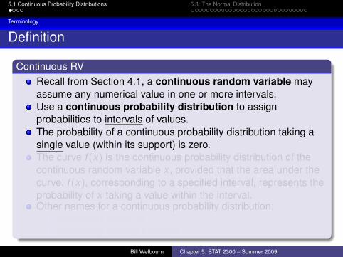
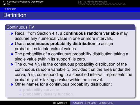
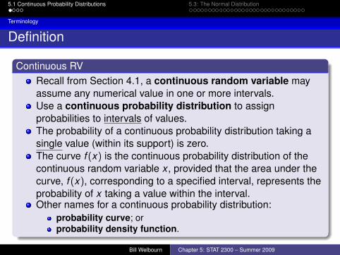
Continuous RVRecall from Section 4.1, a continuous random variable mayassume any numerical value in one or more intervals.Use a continuous probability distribution to assignprobabilities to intervals of values.The probability of a continuous probability distribution taking asingle value (within its support) is zero.The curve f (x) is the continuous probability distribution of thecontinuous random variable x , provided that the area under thecurve, f (x), corresponding to a specified interval, represents theprobability of x taking a value within the interval.Other names for a continuous probability distribution:
probability curve; orprobability density function.
Bill Welbourn Chapter 5: STAT 2300 – Summer 2009

5.1 Continuous Probability Distributions 5.3: The Normal Distribution
Terminology
Definition
Continuous RVRecall from Section 4.1, a continuous random variable mayassume any numerical value in one or more intervals.Use a continuous probability distribution to assignprobabilities to intervals of values.The probability of a continuous probability distribution taking asingle value (within its support) is zero.The curve f (x) is the continuous probability distribution of thecontinuous random variable x , provided that the area under thecurve, f (x), corresponding to a specified interval, represents theprobability of x taking a value within the interval.Other names for a continuous probability distribution:
probability curve; orprobability density function.
Bill Welbourn Chapter 5: STAT 2300 – Summer 2009
5.1 Continuous Probability Distributions 5.3: The Normal Distribution
Terminology
Properties of a Continuous RV
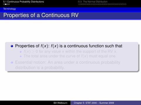
Properties of f (x): f (x) is a continuous function such thatf (x) ≥ 0 for any value x within the support of the RV x .The total area under the curve of f (x) must equal one.
Essential notion: An area under a continuous probabilitydistribution is a probability.
Bill Welbourn Chapter 5: STAT 2300 – Summer 2009

5.1 Continuous Probability Distributions 5.3: The Normal Distribution
Terminology
Properties of a Continuous RV
Properties of f (x): f (x) is a continuous function such thatf (x) ≥ 0 for any value x within the support of the RV x .The total area under the curve of f (x) must equal one.
Essential notion: An area under a continuous probabilitydistribution is a probability.
Bill Welbourn Chapter 5: STAT 2300 – Summer 2009

5.1 Continuous Probability Distributions 5.3: The Normal Distribution
Terminology
Area and Probability
The blue-colored area under the probability curve f (x), from the valuex = a, to x = b, is the probability that x could take any value withinthe interval, [a,b].
Symbolically, P(a ≤ x ≤ b).Equivalently, P(a < x < b). To see this, it holds
P(a ≤ x ≤ b) = P(x = a)︸ ︷︷ ︸=0
+P(a < x < b) + P(x = b)︸ ︷︷ ︸=0
= P(a < x < b).
Bill Welbourn Chapter 5: STAT 2300 – Summer 2009

5.1 Continuous Probability Distributions 5.3: The Normal Distribution
Terminology
Distribution Shapes
Symmetrical and Rectangular
The uniform distribution: Section 5.2.
Symmetrical and Bell-ShapedThe normal distribution: Section 5.3.
SkewedEither left or right: Section 5.5 for the right-skewed exponentialdistribution.
Bill Welbourn Chapter 5: STAT 2300 – Summer 2009
5.1 Continuous Probability Distributions 5.3: The Normal Distribution
Outline
1 5.1 Continuous Probability Distributions
2 5.3: The Normal DistributionPropertiesNormal ProbabilitiesThe Standard Normal Distribution, N(0,1)The Standard Normal TableFinding Normal ProbabilitiesInverse Normal CalculationsThe Tolerance IntervalLinear Interpolation (Optional)
Bill Welbourn Chapter 5: STAT 2300 – Summer 2009
5.1 Continuous Probability Distributions 5.3: The Normal Distribution
Properties
The Normal Probability Distribution, N(µ, σ)
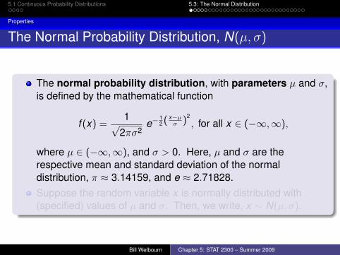
The normal probability distribution, with parameters µ and σ,is defined by the mathematical function
f (x) =1√
2πσ2e−
12(
x−µσ )
2
, for all x ∈ (−∞,∞),
where µ ∈ (−∞,∞), and σ > 0. Here, µ and σ are therespective mean and standard deviation of the normaldistribution, π ≈ 3.14159, and e ≈ 2.71828.Suppose the random variable x is normally distributed with(specified) values of µ and σ. Then, we write, x ∼ N(µ, σ).
Bill Welbourn Chapter 5: STAT 2300 – Summer 2009

5.1 Continuous Probability Distributions 5.3: The Normal Distribution
Properties
The Normal Probability Distribution, N(µ, σ)
The normal probability distribution, with parameters µ and σ,is defined by the mathematical function
f (x) =1√
2πσ2e−
12(
x−µσ )
2
, for all x ∈ (−∞,∞),
where µ ∈ (−∞,∞), and σ > 0. Here, µ and σ are therespective mean and standard deviation of the normaldistribution, π ≈ 3.14159, and e ≈ 2.71828.Suppose the random variable x is normally distributed with(specified) values of µ and σ. Then, we write, x ∼ N(µ, σ).
Bill Welbourn Chapter 5: STAT 2300 – Summer 2009

5.1 Continuous Probability Distributions 5.3: The Normal Distribution
Properties
Properties of the Normal Distribution
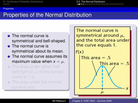
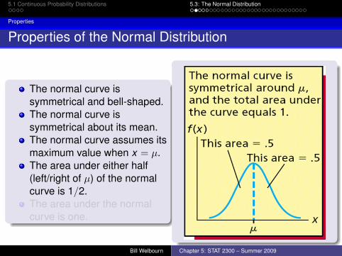
The normal curve issymmetrical and bell-shaped.The normal curve issymmetrical about its mean.The normal curve assumes itsmaximum value when x = µ.The area under either half(left/right of µ) of the normalcurve is 1/2.The area under the normalcurve is one.
Bill Welbourn Chapter 5: STAT 2300 – Summer 2009

5.1 Continuous Probability Distributions 5.3: The Normal Distribution
Properties
Properties of the Normal Distribution
The normal curve issymmetrical and bell-shaped.The normal curve issymmetrical about its mean.The normal curve assumes itsmaximum value when x = µ.The area under either half(left/right of µ) of the normalcurve is 1/2.The area under the normalcurve is one.
Bill Welbourn Chapter 5: STAT 2300 – Summer 2009

5.1 Continuous Probability Distributions 5.3: The Normal Distribution
Properties
Properties of the Normal Distribution (cont.)
There are an infinite number of possible normal distributions.The (numerical) specification of the mean (µ) and standarddeviation (σ) parameters, uniquely identifies a normaldistribution and its shape.The highest point of the normal curve is located at its mean.mean = median = mode. That is, all of the measures of centraltendency (review Section 2.2) equal each other.
Bill Welbourn Chapter 5: STAT 2300 – Summer 2009
5.1 Continuous Probability Distributions 5.3: The Normal Distribution
Properties
Properties of the Normal Distribution (cont.)
The curve is symmetrical about its mean.The left and right halves of the curve are mirror images of eachother.The tails of any normal curve extend to infinity in both directions.
The tails get closer to the horizontal axis as the curve extends offto ±∞, but the curve never touches the axis (Recall, in Section5.1, we require f (x) ≥ 0 for all x).
The area under the normal curve to the right of the mean equalsthe area under the normal curve to the left of the mean.
The area under each half of the curve is 1/2.
Bill Welbourn Chapter 5: STAT 2300 – Summer 2009
5.1 Continuous Probability Distributions 5.3: The Normal Distribution
Properties
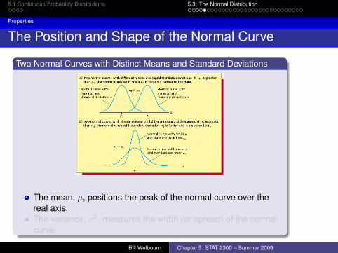
The Position and Shape of the Normal Curve
Two Normal Curves with Distinct Means and Standard Deviations
The mean, µ, positions the peak of the normal curve over thereal axis.The variance, σ2, measures the width (or spread) of the normalcurve.
Bill Welbourn Chapter 5: STAT 2300 – Summer 2009

5.1 Continuous Probability Distributions 5.3: The Normal Distribution
Properties
The Position and Shape of the Normal Curve
Two Normal Curves with Distinct Means and Standard Deviations
The mean, µ, positions the peak of the normal curve over thereal axis.The variance, σ2, measures the width (or spread) of the normalcurve.
Bill Welbourn Chapter 5: STAT 2300 – Summer 2009
5.1 Continuous Probability Distributions 5.3: The Normal Distribution
Normal Probabilities
Normal Probabilities
Suppose x is a normally distributed random variable with mean,µ, and standard deviation, σ. That is, x ∼ N(µ, σ).The probability that x could take any value in the range betweentwo given values, say a and b, where a < b, is P(a ≤ x ≤ b).
P(a ≤ x ≤ b) is the area coloredin blue under the normal curve, forx lying within the interval, [a,b].
Bill Welbourn Chapter 5: STAT 2300 – Summer 2009

5.1 Continuous Probability Distributions 5.3: The Normal Distribution
Normal Probabilities
Three Important Probabilities for the NormalDistribution (Empirical Result)
The 68%− 95%− 99.7% RuleApproximately 68.26% of all possible observed values of x liewithin (plus or minus) one standard deviation of µ. That is,
P(|x − µ| ≤ σ) = P(µ− σ ≤ x ≤ µ+ σ) = 0.6826.
Approximately 95.44% of all possible observed values of x liewithin (plus or minus) two standard deviations of µ. That is,
P(|x − µ| ≤ 2σ) = P(µ− 2σ ≤ x ≤ µ+ 2σ) = 0.9544.
Approximately 99.73% of all possible observed values of x liewithin (plus or minus) three standard deviations of µ. That is,
P(|x − µ| ≤ 3σ) = P(µ− 3σ ≤ x ≤ µ+ 3σ) = 0.9973.
Bill Welbourn Chapter 5: STAT 2300 – Summer 2009

5.1 Continuous Probability Distributions 5.3: The Normal Distribution
Normal Probabilities
Three Important Probabilities for the NormalDistribution (Visual Result)
The 68%− 95%− 99.7% Rule
Bill Welbourn Chapter 5: STAT 2300 – Summer 2009
5.1 Continuous Probability Distributions 5.3: The Normal Distribution
The Standard Normal Distribution, N(0, 1)
Standardizing a Normal Random Variable
The N(0,1) Distribution
Suppose x is normally distributed with mean, µ, and standarddeviation, σ (i.e., x ∼ N(µ, σ)). The random variable z, given by
z =x − µσ
,
is normally distributed with mean zero and standard deviationone (i.e., z ∼ N(0,1)). The normal distribution with mean zeroand standard deviation one is called the standard normaldistribution.Because the mean (µ) and standard deviation (σ) each carry thesame units as x , it follows that z is “unit–less”.
Bill Welbourn Chapter 5: STAT 2300 – Summer 2009
5.1 Continuous Probability Distributions 5.3: The Normal Distribution
The Standard Normal Distribution, N(0, 1)
Relationship Between the Random Variables x and z
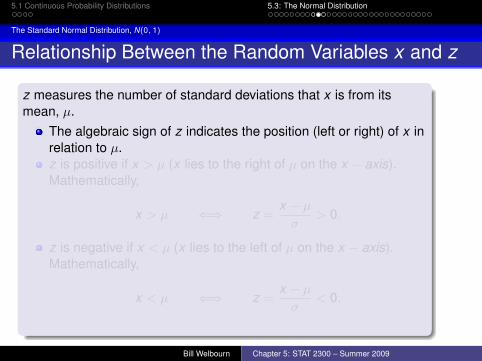
z measures the number of standard deviations that x is from itsmean, µ.
The algebraic sign of z indicates the position (left or right) of x inrelation to µ.z is positive if x > µ (x lies to the right of µ on the x − axis).Mathematically,
x > µ ⇐⇒ z =x − µσ
> 0.
z is negative if x < µ (x lies to the left of µ on the x − axis).Mathematically,
x < µ ⇐⇒ z =x − µσ
< 0.
Bill Welbourn Chapter 5: STAT 2300 – Summer 2009

5.1 Continuous Probability Distributions 5.3: The Normal Distribution
The Standard Normal Distribution, N(0, 1)
Relationship Between the Random Variables x and z
z measures the number of standard deviations that x is from itsmean, µ.
The algebraic sign of z indicates the position (left or right) of x inrelation to µ.z is positive if x > µ (x lies to the right of µ on the x − axis).Mathematically,
x > µ ⇐⇒ z =x − µσ
> 0.
z is negative if x < µ (x lies to the left of µ on the x − axis).Mathematically,
x < µ ⇐⇒ z =x − µσ
< 0.
Bill Welbourn Chapter 5: STAT 2300 – Summer 2009

5.1 Continuous Probability Distributions 5.3: The Normal Distribution
The Standard Normal Distribution, N(0, 1)
Relationship Between the Random Variables x and z(cont.)
Bill Welbourn Chapter 5: STAT 2300 – Summer 2009

5.1 Continuous Probability Distributions 5.3: The Normal Distribution
The Standard Normal Table
The Standard Normal Table
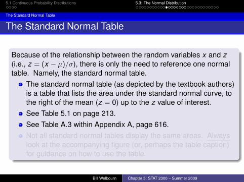
Because of the relationship between the random variables x and z(i.e., z = (x − µ)/σ), there is only the need to reference one normaltable. Namely, the standard normal table.
The standard normal table (as depicted by the textbook authors)is a table that lists the area under the standard normal curve, tothe right of the mean (z = 0) up to the z value of interest.See Table 5.1 on page 213.See Table A.3 within Appendix A, page 616.Not all standard normal tables display the same areas. Alwayslook at the accompanying figure (or, perhaps the table caption)for guidance on how to use the table.
Bill Welbourn Chapter 5: STAT 2300 – Summer 2009

5.1 Continuous Probability Distributions 5.3: The Normal Distribution
The Standard Normal Table
The Standard Normal Table
Because of the relationship between the random variables x and z(i.e., z = (x − µ)/σ), there is only the need to reference one normaltable. Namely, the standard normal table.
The standard normal table (as depicted by the textbook authors)is a table that lists the area under the standard normal curve, tothe right of the mean (z = 0) up to the z value of interest.See Table 5.1 on page 213.See Table A.3 within Appendix A, page 616.Not all standard normal tables display the same areas. Alwayslook at the accompanying figure (or, perhaps the table caption)for guidance on how to use the table.
Bill Welbourn Chapter 5: STAT 2300 – Summer 2009

5.1 Continuous Probability Distributions 5.3: The Normal Distribution
The Standard Normal Table
The Standard Normal Table (cont.)
The values of z (accurate to the nearest hundredth decimalposition) in the table range from 0.00 to 3.09 in increments of0.01.
Accuracy of z to the tenth decimal position are listed in the far leftcolumn.Accuracy of z to the hundredth decimal position are listed acrossthe top of the table.
The areas under the normal curve to the right of the mean, up toany value of z, are given in the body of the table.
Bill Welbourn Chapter 5: STAT 2300 – Summer 2009
5.1 Continuous Probability Distributions 5.3: The Normal Distribution
The Standard Normal Table
Calculating Probabilities Using the Standard NormalTable
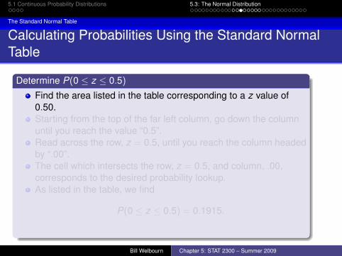
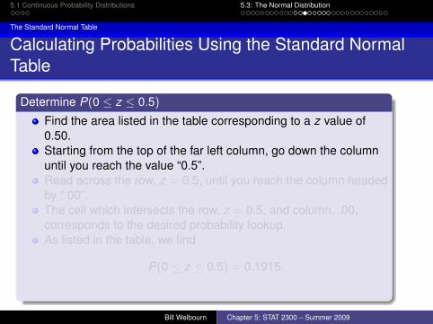
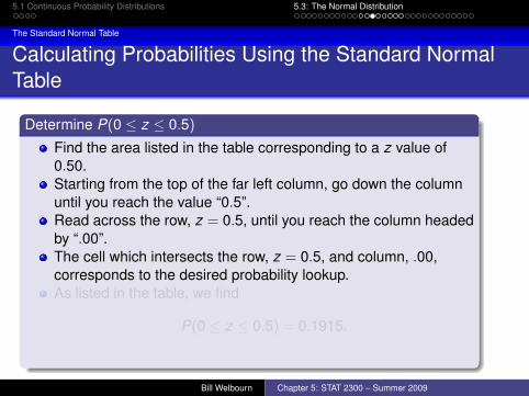
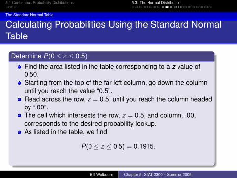
Determine P(0 ≤ z ≤ 0.5)
Find the area listed in the table corresponding to a z value of0.50.Starting from the top of the far left column, go down the columnuntil you reach the value “0.5”.Read across the row, z = 0.5, until you reach the column headedby “.00”.The cell which intersects the row, z = 0.5, and column, .00,corresponds to the desired probability lookup.As listed in the table, we find
P(0 ≤ z ≤ 0.5) = 0.1915.
Bill Welbourn Chapter 5: STAT 2300 – Summer 2009
5.1 Continuous Probability Distributions 5.3: The Normal Distribution
The Standard Normal Table
Calculating Probabilities Using the Standard NormalTable
Determine P(0 ≤ z ≤ 0.5)
Find the area listed in the table corresponding to a z value of0.50.Starting from the top of the far left column, go down the columnuntil you reach the value “0.5”.Read across the row, z = 0.5, until you reach the column headedby “.00”.The cell which intersects the row, z = 0.5, and column, .00,corresponds to the desired probability lookup.As listed in the table, we find
P(0 ≤ z ≤ 0.5) = 0.1915.
Bill Welbourn Chapter 5: STAT 2300 – Summer 2009
5.1 Continuous Probability Distributions 5.3: The Normal Distribution
The Standard Normal Table
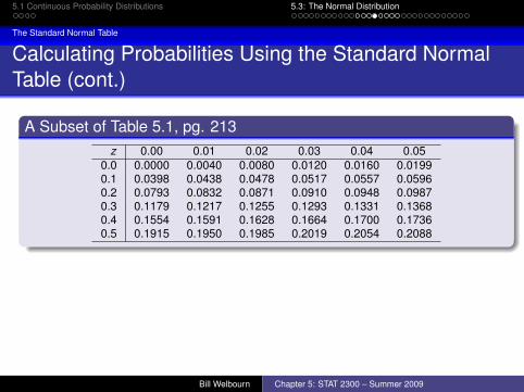
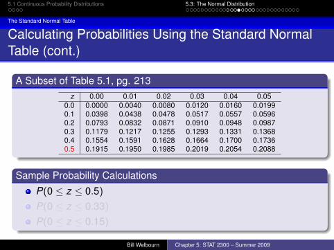
Calculating Probabilities Using the Standard NormalTable (cont.)
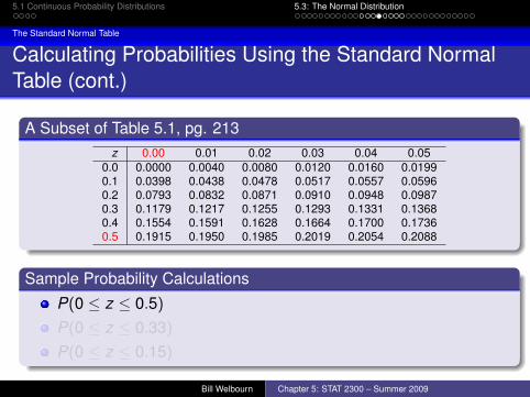
A Subset of Table 5.1, pg. 213z 0.00 0.01 0.02 0.03 0.04 0.05
0.0 0.0000 0.0040 0.0080 0.0120 0.0160 0.01990.1 0.0398 0.0438 0.0478 0.0517 0.0557 0.05960.2 0.0793 0.0832 0.0871 0.0910 0.0948 0.09870.3 0.1179 0.1217 0.1255 0.1293 0.1331 0.13680.4 0.1554 0.1591 0.1628 0.1664 0.1700 0.17360.5 0.1915 0.1950 0.1985 0.2019 0.2054 0.2088
Sample Probability Calculations
P(0 ≤ z ≤ 0.5)
= 0.1915.
P(0 ≤ z ≤ 0.33)
= 0.1293.
P(0 ≤ z ≤ 0.15)
= 0.0596.
Bill Welbourn Chapter 5: STAT 2300 – Summer 2009

5.1 Continuous Probability Distributions 5.3: The Normal Distribution
The Standard Normal Table
Calculating Probabilities Using the Standard NormalTable (cont.)
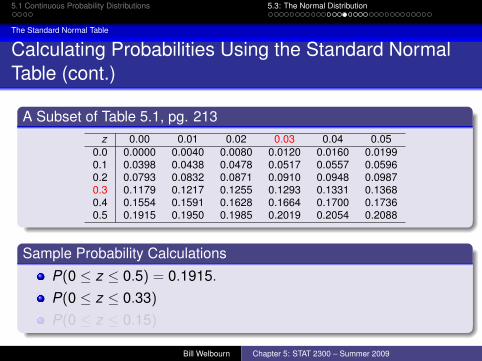
A Subset of Table 5.1, pg. 213z 0.00 0.01 0.02 0.03 0.04 0.05
0.0 0.0000 0.0040 0.0080 0.0120 0.0160 0.01990.1 0.0398 0.0438 0.0478 0.0517 0.0557 0.05960.2 0.0793 0.0832 0.0871 0.0910 0.0948 0.09870.3 0.1179 0.1217 0.1255 0.1293 0.1331 0.13680.4 0.1554 0.1591 0.1628 0.1664 0.1700 0.17360.5 0.1915 0.1950 0.1985 0.2019 0.2054 0.2088
Sample Probability Calculations
P(0 ≤ z ≤ 0.5)
= 0.1915.
P(0 ≤ z ≤ 0.33)
= 0.1293.
P(0 ≤ z ≤ 0.15)
= 0.0596.
Bill Welbourn Chapter 5: STAT 2300 – Summer 2009
5.1 Continuous Probability Distributions 5.3: The Normal Distribution
The Standard Normal Table
Calculating Probabilities Using the Standard NormalTable (cont.)
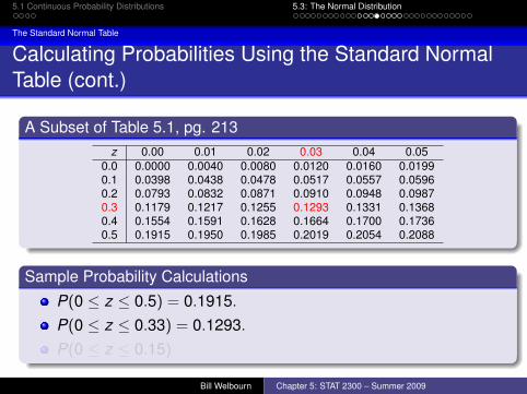
A Subset of Table 5.1, pg. 213z 0.00 0.01 0.02 0.03 0.04 0.05
0.0 0.0000 0.0040 0.0080 0.0120 0.0160 0.01990.1 0.0398 0.0438 0.0478 0.0517 0.0557 0.05960.2 0.0793 0.0832 0.0871 0.0910 0.0948 0.09870.3 0.1179 0.1217 0.1255 0.1293 0.1331 0.13680.4 0.1554 0.1591 0.1628 0.1664 0.1700 0.17360.5 0.1915 0.1950 0.1985 0.2019 0.2054 0.2088
Sample Probability Calculations
P(0 ≤ z ≤ 0.5)
= 0.1915.
P(0 ≤ z ≤ 0.33)
= 0.1293.
P(0 ≤ z ≤ 0.15)
= 0.0596.
Bill Welbourn Chapter 5: STAT 2300 – Summer 2009
5.1 Continuous Probability Distributions 5.3: The Normal Distribution
The Standard Normal Table
Calculating Probabilities Using the Standard NormalTable (cont.)
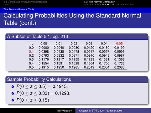
A Subset of Table 5.1, pg. 213z 0.00 0.01 0.02 0.03 0.04 0.05
0.0 0.0000 0.0040 0.0080 0.0120 0.0160 0.01990.1 0.0398 0.0438 0.0478 0.0517 0.0557 0.05960.2 0.0793 0.0832 0.0871 0.0910 0.0948 0.09870.3 0.1179 0.1217 0.1255 0.1293 0.1331 0.13680.4 0.1554 0.1591 0.1628 0.1664 0.1700 0.17360.5 0.1915 0.1950 0.1985 0.2019 0.2054 0.2088
Sample Probability Calculations
P(0 ≤ z ≤ 0.5)
= 0.1915.
P(0 ≤ z ≤ 0.33)
= 0.1293.
P(0 ≤ z ≤ 0.15)
= 0.0596.
Bill Welbourn Chapter 5: STAT 2300 – Summer 2009

5.1 Continuous Probability Distributions 5.3: The Normal Distribution
The Standard Normal Table
Calculating Probabilities Using the Standard NormalTable (cont.)
A Subset of Table 5.1, pg. 213z 0.00 0.01 0.02 0.03 0.04 0.05
0.0 0.0000 0.0040 0.0080 0.0120 0.0160 0.01990.1 0.0398 0.0438 0.0478 0.0517 0.0557 0.05960.2 0.0793 0.0832 0.0871 0.0910 0.0948 0.09870.3 0.1179 0.1217 0.1255 0.1293 0.1331 0.13680.4 0.1554 0.1591 0.1628 0.1664 0.1700 0.17360.5 0.1915 0.1950 0.1985 0.2019 0.2054 0.2088
Sample Probability Calculations
P(0 ≤ z ≤ 0.5) = 0.1915.P(0 ≤ z ≤ 0.33)
= 0.1293.
P(0 ≤ z ≤ 0.15)
= 0.0596.
Bill Welbourn Chapter 5: STAT 2300 – Summer 2009
5.1 Continuous Probability Distributions 5.3: The Normal Distribution
The Standard Normal Table
Calculating Probabilities Using the Standard NormalTable (cont.)
A Subset of Table 5.1, pg. 213z 0.00 0.01 0.02 0.03 0.04 0.05
0.0 0.0000 0.0040 0.0080 0.0120 0.0160 0.01990.1 0.0398 0.0438 0.0478 0.0517 0.0557 0.05960.2 0.0793 0.0832 0.0871 0.0910 0.0948 0.09870.3 0.1179 0.1217 0.1255 0.1293 0.1331 0.13680.4 0.1554 0.1591 0.1628 0.1664 0.1700 0.17360.5 0.1915 0.1950 0.1985 0.2019 0.2054 0.2088
Sample Probability Calculations
P(0 ≤ z ≤ 0.5) = 0.1915.P(0 ≤ z ≤ 0.33) = 0.1293.P(0 ≤ z ≤ 0.15)
= 0.0596.
Bill Welbourn Chapter 5: STAT 2300 – Summer 2009

5.1 Continuous Probability Distributions 5.3: The Normal Distribution
The Standard Normal Table
Calculating Probabilities Using the Standard NormalTable (cont.)
A Subset of Table 5.1, pg. 213z 0.00 0.01 0.02 0.03 0.04 0.05
0.0 0.0000 0.0040 0.0080 0.0120 0.0160 0.01990.1 0.0398 0.0438 0.0478 0.0517 0.0557 0.05960.2 0.0793 0.0832 0.0871 0.0910 0.0948 0.09870.3 0.1179 0.1217 0.1255 0.1293 0.1331 0.13680.4 0.1554 0.1591 0.1628 0.1664 0.1700 0.17360.5 0.1915 0.1950 0.1985 0.2019 0.2054 0.2088
Sample Probability Calculations
P(0 ≤ z ≤ 0.5) = 0.1915.P(0 ≤ z ≤ 0.33) = 0.1293.P(0 ≤ z ≤ 0.15) = 0.0596.
Bill Welbourn Chapter 5: STAT 2300 – Summer 2009

5.1 Continuous Probability Distributions 5.3: The Normal Distribution
The Standard Normal Table
Figure 5.9, pg. 214
The Symmetry of the Standard Normal Distribution
Bill Welbourn Chapter 5: STAT 2300 – Summer 2009

5.1 Continuous Probability Distributions 5.3: The Normal Distribution
The Standard Normal Table
Calculate: P(−2.53 ≤ z ≤ 2.53)
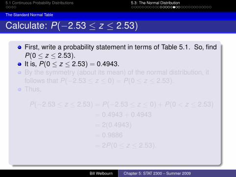
First, write a probability statement in terms of Table 5.1. So, findP(0 ≤ z ≤ 2.53).It is, P(0 ≤ z ≤ 2.53) = 0.4943.By the symmetry (about its mean) of the normal distribution, itfollows that P(−2.53 ≤ z ≤ 0) = P(0 ≤ z ≤ 2.53).Thus,
P(−2.53 ≤ z ≤ 2.53) = P(−2.53 ≤ z ≤ 0) + P(0 < z ≤ 2.53)
= 0.4943 + 0.4943= 2(0.4943)
= 0.9886= 2P(0 ≤ z ≤ 2.53).
Bill Welbourn Chapter 5: STAT 2300 – Summer 2009
5.1 Continuous Probability Distributions 5.3: The Normal Distribution
The Standard Normal Table
Calculate: P(−2.53 ≤ z ≤ 2.53)
First, write a probability statement in terms of Table 5.1. So, findP(0 ≤ z ≤ 2.53).It is, P(0 ≤ z ≤ 2.53) = 0.4943.By the symmetry (about its mean) of the normal distribution, itfollows that P(−2.53 ≤ z ≤ 0) = P(0 ≤ z ≤ 2.53).Thus,
P(−2.53 ≤ z ≤ 2.53) = P(−2.53 ≤ z ≤ 0) + P(0 < z ≤ 2.53)
= 0.4943 + 0.4943= 2(0.4943)
= 0.9886= 2P(0 ≤ z ≤ 2.53).
Bill Welbourn Chapter 5: STAT 2300 – Summer 2009
5.1 Continuous Probability Distributions 5.3: The Normal Distribution
The Standard Normal Table
Calculate: P(z ≥ −1)
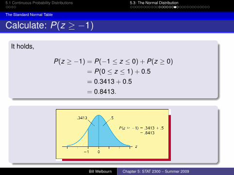
It holds,
P(z ≥ −1) = P(−1 ≤ z ≤ 0) + P(z ≥ 0)
= P(0 ≤ z ≤ 1) + 0.5= 0.3413 + 0.5= 0.8413.
Bill Welbourn Chapter 5: STAT 2300 – Summer 2009

5.1 Continuous Probability Distributions 5.3: The Normal Distribution
The Standard Normal Table
Calculate: P(z ≥ 1)
Method OneIt holds,
P(z ≥ 1) = 1− P(z < 1)
= 1− [P(z < 0) + P(0 ≤ z < 1)]
= 1− (0.5 + 0.3413)
= 0.5− 0.3413= 0.1587.
Method TwoIt holds,
P(z ≥ 1) = P(z ≥ 0)− P(0 ≤ z < 1)
= 0.5− 0.3413= 0.1587.
Bill Welbourn Chapter 5: STAT 2300 – Summer 2009

5.1 Continuous Probability Distributions 5.3: The Normal Distribution
Finding Normal Probabilities
Finding Normal Probabilities
General ProcedureFormulate the problem in terms of x values.Calculate the corresponding z values, and restate the problem interms of these z values.Find the required areas under the standard normal curve byusing the table.Note: It is always useful to draw a picture showing the requiredareas before using the normal table.
Bill Welbourn Chapter 5: STAT 2300 – Summer 2009
5.1 Continuous Probability Distributions 5.3: The Normal Distribution
Finding Normal Probabilities
Example 5.2, pg. 217
ProblemWe want the probability that the mileage of a randomly selectedmidsize car will be between 32 and 35 mpg.
Solution SetupLet x be the random variable of mileage of midsize cars, in mpg.Given: x ∼ N(33 mpg,0.7 mpg).We need to find, P(32 mpg ≤ x ≤ 35mpg).
Bill Welbourn Chapter 5: STAT 2300 – Summer 2009

5.1 Continuous Probability Distributions 5.3: The Normal Distribution
Finding Normal Probabilities
Example 5.2 (cont.)
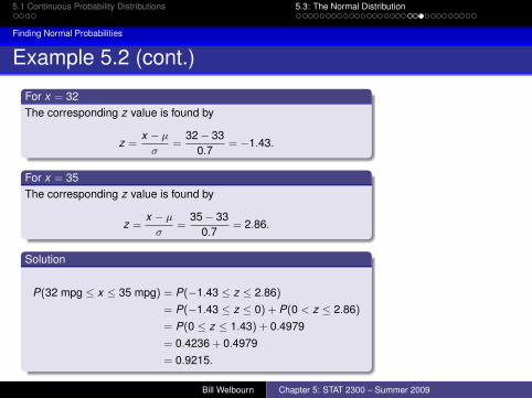
For x = 32The corresponding z value is found by
z =x − µσ
=32− 33
0.7= −1.43.
For x = 35The corresponding z value is found by
z =x − µσ
=35− 33
0.7= 2.86.
Solution
P(32 mpg ≤ x ≤ 35 mpg) = P(−1.43 ≤ z ≤ 2.86)
= P(−1.43 ≤ z ≤ 0) + P(0 < z ≤ 2.86)
= P(0 ≤ z ≤ 1.43) + 0.4979= 0.4236 + 0.4979= 0.9215.
Bill Welbourn Chapter 5: STAT 2300 – Summer 2009

5.1 Continuous Probability Distributions 5.3: The Normal Distribution
Finding Normal Probabilities
Example 5.2 (cont.)
For x = 32The corresponding z value is found by
z =x − µσ
=32− 33
0.7= −1.43.
For x = 35The corresponding z value is found by
z =x − µσ
=35− 33
0.7= 2.86.
Solution
P(32 mpg ≤ x ≤ 35 mpg) = P(−1.43 ≤ z ≤ 2.86)
= P(−1.43 ≤ z ≤ 0) + P(0 < z ≤ 2.86)
= P(0 ≤ z ≤ 1.43) + 0.4979= 0.4236 + 0.4979= 0.9215.
Bill Welbourn Chapter 5: STAT 2300 – Summer 2009

5.1 Continuous Probability Distributions 5.3: The Normal Distribution
Inverse Normal Calculations
Finding z Values on a Standard Normal Curve
Notation, pg. 221For the standard normal distribution, let zα denote the point onthe horizontal axis which yields a right-hand tail area equal to α.The figure shown below, demonstrates how to find zα forα = 0.025.
The Point z0.025 = 1.96
Bill Welbourn Chapter 5: STAT 2300 – Summer 2009

5.1 Continuous Probability Distributions 5.3: The Normal Distribution
Inverse Normal Calculations
Example 5.5, pg. 221
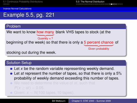
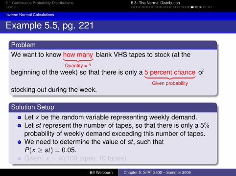
ProblemWe want to know how many︸ ︷︷ ︸
Quantity = ?
blank VHS tapes to stock (at the
beginning of the week) so that there is only a 5 percent chance︸ ︷︷ ︸
Given probability
of
stocking out during the week.
Solution SetupLet x be the random variable representing weekly demand.Let st represent the number of tapes, so that there is only a 5%probability of weekly demand exceeding this number of tapes.We need to determine the value of st , such thatP(x ≥ st) = 0.05.Given: x ∼ N(100 tapes,10 tapes).
Bill Welbourn Chapter 5: STAT 2300 – Summer 2009

5.1 Continuous Probability Distributions 5.3: The Normal Distribution
Inverse Normal Calculations
Example 5.5, pg. 221
ProblemWe want to know how many︸ ︷︷ ︸
Quantity = ?
blank VHS tapes to stock (at the
beginning of the week) so that there is only a 5 percent chance︸ ︷︷ ︸Given probability
of
stocking out during the week.
Solution SetupLet x be the random variable representing weekly demand.Let st represent the number of tapes, so that there is only a 5%probability of weekly demand exceeding this number of tapes.We need to determine the value of st , such thatP(x ≥ st) = 0.05.Given: x ∼ N(100 tapes,10 tapes).
Bill Welbourn Chapter 5: STAT 2300 – Summer 2009
5.1 Continuous Probability Distributions 5.3: The Normal Distribution
Inverse Normal Calculations
Example 5.5, pg. 221 (cont.)
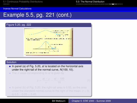
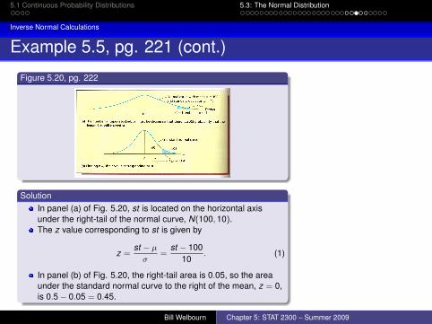
Figure 5.20, pg. 222
SolutionIn panel (a) of Fig. 5.20, st is located on the horizontal axisunder the right-tail of the normal curve, N(100,10).The z value corresponding to st is given by
z =st − µσ
=st − 100
10. (1)
In panel (b) of Fig. 5.20, the right-tail area is 0.05, so the areaunder the standard normal curve to the right of the mean, z = 0,is 0.5− 0.05 = 0.45.
Bill Welbourn Chapter 5: STAT 2300 – Summer 2009

5.1 Continuous Probability Distributions 5.3: The Normal Distribution
Inverse Normal Calculations
Example 5.5, pg. 221 (cont.)
Figure 5.20, pg. 222
SolutionIn panel (a) of Fig. 5.20, st is located on the horizontal axisunder the right-tail of the normal curve, N(100,10).The z value corresponding to st is given by
z =st − µσ
=st − 100
10. (1)
In panel (b) of Fig. 5.20, the right-tail area is 0.05, so the areaunder the standard normal curve to the right of the mean, z = 0,is 0.5− 0.05 = 0.45.
Bill Welbourn Chapter 5: STAT 2300 – Summer 2009

5.1 Continuous Probability Distributions 5.3: The Normal Distribution
Inverse Normal Calculations
Example 5.5, pg. 221 (cont.)
Solution (cont.)Use the standard normal table to find the value of z (outer portion ofthe table), corresponding with a table entry of 0.45 (inner portion ofthe table).
But do not find 0.45 (this value is not given in the table); insteadfind values which bracket (flank) that of 0.45.For a table entry (area) of 0.4495, z = 1.64.For a table entry (area) of 0.4505, z = 1.65.For an area of 0.45, use the z value midway between the valuesof 1.64 and 1.65 (see the linear interpolation slides at the end ofthis module).So, z0.05 = 1.645 (approximately).
Bill Welbourn Chapter 5: STAT 2300 – Summer 2009

5.1 Continuous Probability Distributions 5.3: The Normal Distribution
Inverse Normal Calculations
Example 5.5, pg. 221 (cont.)
Solution (cont.)Since z0.05 = 1.645, by (1), it follows that
1.645 =st − 100
10.
Solving for st , we have
st = 100 + (1.645)(10) = 116.45.
Rounding up, 117 tapes should be stocked so that the probabilityof running out will not be more than 5 percent.
Bill Welbourn Chapter 5: STAT 2300 – Summer 2009

5.1 Continuous Probability Distributions 5.3: The Normal Distribution
The Tolerance Interval
Finding a Tolerance Interval
Setup
Given a normal distribution, N(µ, σ), and a specified value of α,α ∈ (0,1), consider computing a tolerance interval (denoted by[µ± kσ] ) which contains 100(1− α)% of the measurements for thisnormal distribution.
Steps for Finding k
Let [x1, x2] denote the tolerance interval.It follows that
z2 =x2 − µσ
=µ+ kσ − µ
σ= k .
But, (α/2)% of the measurements must fall to the right of x2 (andso also z2).Hence, z2 = k = zα/2.
Bill Welbourn Chapter 5: STAT 2300 – Summer 2009
5.1 Continuous Probability Distributions 5.3: The Normal Distribution
The Tolerance Interval
Tolerance Interval Example
90% Tolerance IntervalFrom the previous slide, k = zα/2.Here, 1− α = 0.90, so that α = 0.10.We previously found (using linear interpolation) thatz0.05 ≈ 1.645.Therefore, [µ± 1.645σ] is a 90% tolerance interval for a normaldistribution with mean, µ, and standard deviation, σ.
Bill Welbourn Chapter 5: STAT 2300 – Summer 2009

5.1 Continuous Probability Distributions 5.3: The Normal Distribution
Linear Interpolation (Optional)
Linear Interpolation (Optional)
Point Slope Formula, y = m(x − x0) + y0
Consider the two points, (x0, y0) and (x1, y1), which lie on theline.The slope, m, satisfies the equation
m =y1 − y0
x1 − x0
It can be shown that any third point on the line, say (x2, y2),satisfies
x2 = x0 + (y2 − y0)(m)−1, for m 6= 0. (2)
Bill Welbourn Chapter 5: STAT 2300 – Summer 2009

5.1 Continuous Probability Distributions 5.3: The Normal Distribution
Linear Interpolation (Optional)
Linear Interpolation (Optional)
ApplicationFrom Table 5.1 (pg. 213), we find
P(0 ≤ z ≤ 1.64) = 0.4495 and P(0 ≤ z ≤ 1.65) = 0.4505.(3)
Let (x0, y0) = (1.64,0.4495) and (x1, y1) = (1.65,0.4505),corresponding to the probabilities given by (3). Consider theordered pair, (x2, y2 = 0.45), where x2 satisfies
P(0 ≤ z ≤ x2) = 0.45.
By (2), it is
x2 = 1.64 + (0.45− 0.4495)(1.65− 1.64)/(0.4505− 0.4495) = 1.645.
This implies that P(0 ≤ z ≤ 1.645) ≈ 0.45.Therefore, utilizing linear interpolation, we find that z0.05 ≈ 1.645.
Bill Welbourn Chapter 5: STAT 2300 – Summer 2009
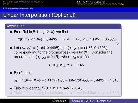
5.1 Continuous Probability Distributions 5.3: The Normal Distribution
Linear Interpolation (Optional)
Linear Interpolation (Optional)
ApplicationFrom Table 5.1 (pg. 213), we find
P(0 ≤ z ≤ 1.64) = 0.4495 and P(0 ≤ z ≤ 1.65) = 0.4505.(3)
Let (x0, y0) = (1.64,0.4495) and (x1, y1) = (1.65,0.4505),corresponding to the probabilities given by (3). Consider theordered pair, (x2, y2 = 0.45), where x2 satisfies
P(0 ≤ z ≤ x2) = 0.45.
By (2), it is
x2 = 1.64 + (0.45− 0.4495)(1.65− 1.64)/(0.4505− 0.4495) = 1.645.
This implies that P(0 ≤ z ≤ 1.645) ≈ 0.45.Therefore, utilizing linear interpolation, we find that z0.05 ≈ 1.645.
Bill Welbourn Chapter 5: STAT 2300 – Summer 2009