robotics ch5
DESCRIPTION
chapter 5TRANSCRIPT
From “Introduction to Robotics” by S.K. Saha Tata McGraw-Hill Publishing Company Limited, New Delhi, 2008
1
Chapter 5 Transformations
For the purpose of controlling a robot, it is necessary to know the relationships between the joints motion (input) and the end-effector motions (output), because the joint motions control the end-effector movements. Thus, the study of kinematics is important, where transformations between the coordinate frames attached to different robot links of the robot need to be performed
5.1 Robot Architecture A robot is made up of several links connected serially by joints. The robot’s degree of freedom (DOF) depends on the number of links and joints, their types, and the kinematic chain of the robot.
5.1.1 Links and joints
The individual bodies that make up a robot are called 'links.' Here, unless otherwise stated, all links are assumed to be rigid, i.e., the distance between any two points within the body does not change while it is moving. A rigid body in the three dimensional Cartesian space has six DOF. This implies that the position of the body can be described by three translational, and the orientation by three rotational coordinates. For convenience, certain non-rigid bodies, such as chains, cables, or belts, which when serve the same function as the rigid bodies, may be considered as links. From the kinamatic point of view, two or more members when connected together without any relative motion between them is considered as a single link. For example, an assembly of two gears connected by a common shaft is treated as one link.
Links of a robot are coupled by kinematic pairs or joints. A 'joint' couples two links and provides physical constraints on the relative motion between the links. It is not a physical entity but just a concept that allows one to specify how one link moves with respect to another one. For example, a hinge joint of a door allows it to move relative to the fixed wall about an axis. No other motion is possible. Type of relative motion permitted by a joint is governed by the form of the contact surface between the members, which can be a surface, a line, or a point. Accordingly, they are termed as either 'lower' or 'higher' pair joint. If two mating links are in surface contact, the joint is referred to as a lower pair joint. On the contrary, if the links are in line or point contact, the joint is called higher pair joint. As per the definition, the hinge joint of the door is a lower pair joint, whereas a ball rolling on a plane makes a higher pair joint. Frequently used lower and higher pairs are listed in Table 5.1.
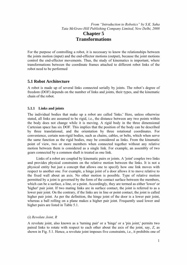
(i) Revolute Joint, R
A revolute joint, also known as a 'turning pair' or a 'hinge' or a 'pin joint,' permits two paired links to rotate with respect to each other about the axis of the joint, say, Z, as shown in Fig. 5.1. Hence, a revolute joint imposes five constraints, i.e., it prohibits one of
From “Introduction to Robotics” by S.K. Saha Tata McGraw-Hill Publishing Company Limited, New Delhi, 2008
2
the links to translate with respect to the other one along the three perpendicular axes, X, Y, Z, along with the rotation about two axes, X and Y. This joint has one-degree- of-freedom (DOF).
(a) Geometrical form (b) Representations
Figure 5.1 A revolute joint
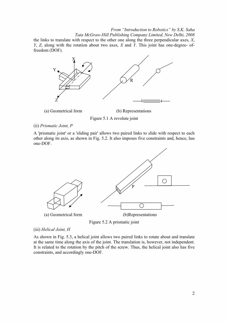
(ii) Prismatic Joint, P
A 'prismatic joint' or a 'sliding pair' allows two paired links to slide with respect to each other along its axis, as shown in Fig. 5.2. It also imposes five constraints and, hence, has one-DOF.
(a) Geometrical form (b)Representations
Figure 5.2 A prismatic joint
(iii) Helical Joint, H
As shown in Fig. 5.3, a helical joint allows two paired links to rotate about and translate at the same time along the axis of the joint. The translation is, however, not independent. It is related to the rotation by the pitch of the screw. Thus, the helical joint also has five constraints, and accordingly one-DOF.
X
Y
Z
R
P
From “Introduction to Robotics” by S.K. Saha Tata McGraw-Hill Publishing Company Limited, New Delhi, 2008
3
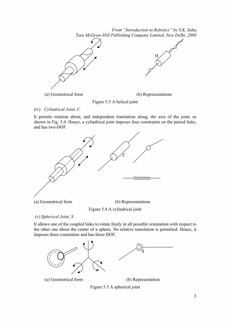
(a) Geometrical form (b) Representations
Figure 5.3 A helical joint
(iv) Cylindrical Joint, C
It permits rotation about, and independent translation along, the axis of the joint, as shown in Fig. 5.4. Hence, a cylindrical joint imposes four constraints on the paired links, and has two-DOF.
(a) Geometrical form (b) Representations
Figure 5.4 A cylindrical joint
(v) Spherical Joint, S
It allows one of the coupled links to rotate freely in all possible orientation with respect to the other one about the center of a sphere. No relative translation is permitted. Hence, it imposes three constraints and has three-DOF.
(a) Geometrical form (b) Representation
Figure 5.5 A spherical joint
C
S
H
From “Introduction to Robotics” by S.K. Saha Tata McGraw-Hill Publishing Company Limited, New Delhi, 2008
4
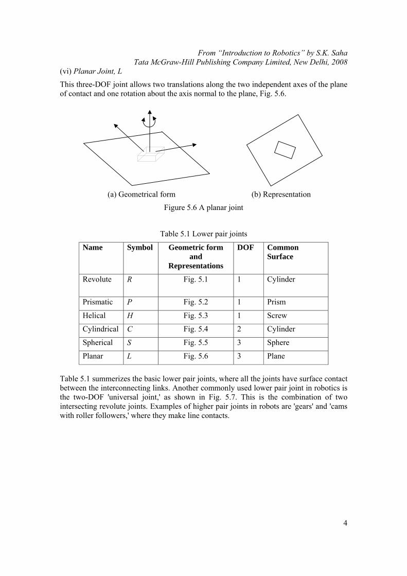
(vi) Planar Joint, L
This three-DOF joint allows two translations along the two independent axes of the plane of contact and one rotation about the axis normal to the plane, Fig. 5.6.
(a) Geometrical form (b) Representation
Figure 5.6 A planar joint
Table 5.1 Lower pair joints
Name Symbol Geometric form and
Representations
DOF Common Surface
Revolute R Fig. 5.1
1 Cylinder
Prismatic P Fig. 5.2 1 Prism
Helical H Fig. 5.3 1 Screw
Cylindrical C Fig. 5.4 2 Cylinder
Spherical S Fig. 5.5 3 Sphere
Planar L Fig. 5.6 3 Plane
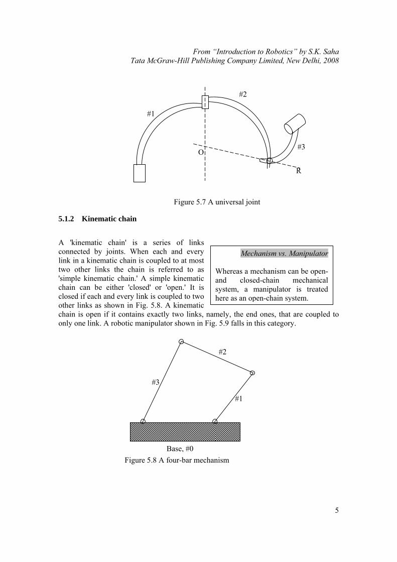
Table 5.1 summerizes the basic lower pair joints, where all the joints have surface contact between the interconnecting links. Another commonly used lower pair joint in robotics is the two-DOF 'universal joint,' as shown in Fig. 5.7. This is the combination of two intersecting revolute joints. Examples of higher pair joints in robots are 'gears' and 'cams with roller followers,' where they make line contacts.
From “Introduction to Robotics” by S.K. Saha Tata McGraw-Hill Publishing Company Limited, New Delhi, 2008
5
Mechanism vs. Manipulator Whereas a mechanism can be open- and closed-chain mechanical system, a manipulator is treated here as an open-chain system.
Figure 5.7 A universal joint
5.1.2 Kinematic chain
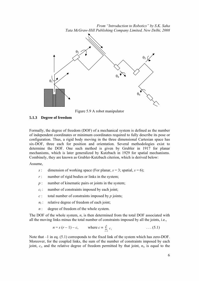
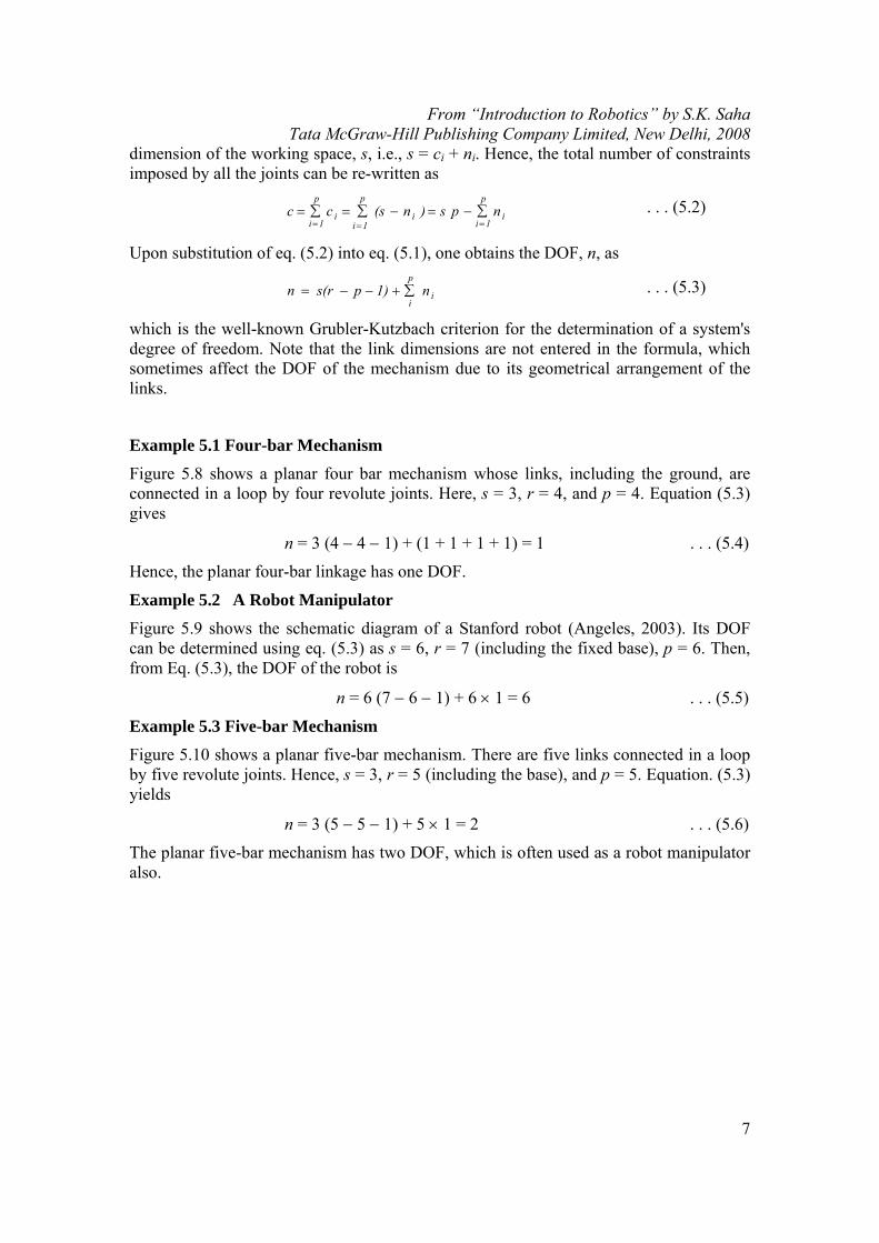
A 'kinematic chain' is a series of links connected by joints. When each and every link in a kinematic chain is coupled to at most two other links the chain is referred to as 'simple kinematic chain.' A simple kinematic chain can be either 'closed' or 'open.' It is closed if each and every link is coupled to two other links as shown in Fig. 5.8. A kinematic chain is open if it contains exactly two links, namely, the end ones, that are coupled to only one link. A robotic manipulator shown in Fig. 5.9 falls in this category.
Figure 5.8 A four-bar mechanism
#1
#2
#3 O
R
Base, #0
#3
#2
#1
From “Introduction to Robotics” by S.K. Saha Tata McGraw-Hill Publishing Company Limited, New Delhi, 2008
6
Figure 5.9 A robot manipulator
5.1.3 Degree of freedom
Formally, the degree of freedom (DOF) of a mechanical system is defined as the number of independent coordinates or minimum coordinates required to fully describe its pose or configuration. Thus, a rigid body moving in the three dimensional Cartesian space has six-DOF, three each for position and orientation. Several methodologies exist to determine the DOF. One such method is given by Grubler in 1917 for planar mechanisms, which is later generalized by Kutzbach in 1929 for spatial mechanisms. Combinely, they are known as Grubler-Kutzbach citerion, which is derived below:
Assume,
s : dimension of working space (For planar, s = 3; spatial, s = 6);
r : number of rigid bodies or links in the system;
p : number of kinematic pairs or joints in the system;
ci : number of constraints imposed by each joint;
c : total number of constraints imposed by p joints;
ni : relative degree of freedom of each joint;
n : degree of freedom of the whole system.
The DOF of the whole system, n, is then determined from the total DOF associated with all the moving links minus the total number of constraints imposed by all the joints, i.e.,
n = s (r − 1) − c, where c ≡ i
1c
p
i=∑ . . . (5.1)
Note that –1 in eq. (5.1) corresponds to the fixed link of the system which has zero-DOF. Moreover, for the coupled links, the sum of the number of constraints imposed by each joint, ci, and the relative degree of freedom permitted by that joint, ni, is equal to the
θ6
θ5
θ4
θ2
θ1
From “Introduction to Robotics” by S.K. Saha Tata McGraw-Hill Publishing Company Limited, New Delhi, 2008
7
dimension of the working space, s, i.e., s = ci + ni. Hence, the total number of constraints imposed by all the joints can be re-written as
i
p
1ii
p
1ii
p
1inps)n(scc
===∑−=−∑=∑= . . . (5.2)
Upon substitution of eq. (5.2) into eq. (5.1), one obtains the DOF, n, as
i
p
in1)ps(rn ∑+−−= . . . (5.3)
which is the well-known Grubler-Kutzbach criterion for the determination of a system's degree of freedom. Note that the link dimensions are not entered in the formula, which sometimes affect the DOF of the mechanism due to its geometrical arrangement of the links.
Example 5.1 Four-bar Mechanism
Figure 5.8 shows a planar four bar mechanism whose links, including the ground, are connected in a loop by four revolute joints. Here, s = 3, r = 4, and p = 4. Equation (5.3) gives
n = 3 (4 − 4 − 1) + (1 + 1 + 1 + 1) = 1 . . . (5.4)
Hence, the planar four-bar linkage has one DOF.
Example 5.2 A Robot Manipulator
Figure 5.9 shows the schematic diagram of a Stanford robot (Angeles, 2003). Its DOF can be determined using eq. (5.3) as s = 6, r = 7 (including the fixed base), p = 6. Then, from Eq. (5.3), the DOF of the robot is
n = 6 (7 − 6 − 1) + 6 × 1 = 6 . . . (5.5)
Example 5.3 Five-bar Mechanism
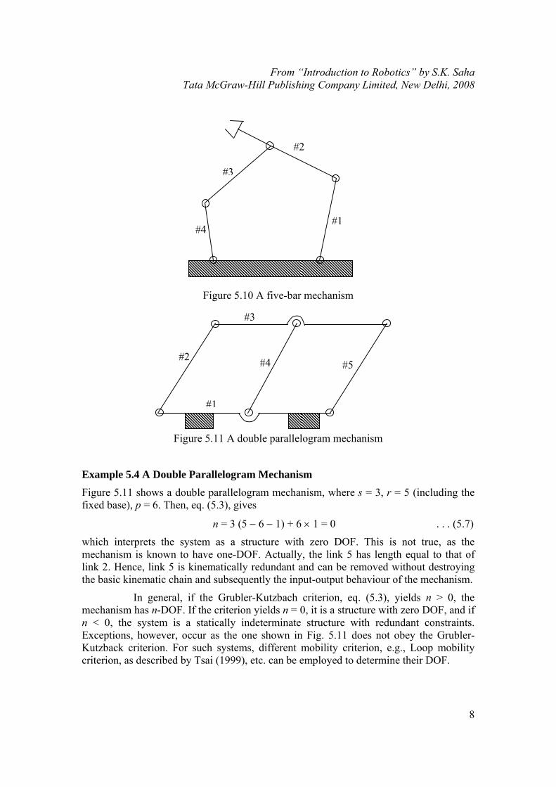
Figure 5.10 shows a planar five-bar mechanism. There are five links connected in a loop by five revolute joints. Hence, s = 3, r = 5 (including the base), and p = 5. Equation. (5.3) yields
n = 3 (5 − 5 − 1) + 5 × 1 = 2 . . . (5.6)
The planar five-bar mechanism has two DOF, which is often used as a robot manipulator also.
From “Introduction to Robotics” by S.K. Saha Tata McGraw-Hill Publishing Company Limited, New Delhi, 2008
8
Figure 5.10 A five-bar mechanism
Figure 5.11 A double parallelogram mechanism
Example 5.4 A Double Parallelogram Mechanism
Figure 5.11 shows a double parallelogram mechanism, where s = 3, r = 5 (including the fixed base), p = 6. Then, eq. (5.3), gives
n = 3 (5 − 6 − 1) + 6 × 1 = 0 . . . (5.7)
which interprets the system as a structure with zero DOF. This is not true, as the mechanism is known to have one-DOF. Actually, the link 5 has length equal to that of link 2. Hence, link 5 is kinematically redundant and can be removed without destroying the basic kinematic chain and subsequently the input-output behaviour of the mechanism.
In general, if the Grubler-Kutzbach criterion, eq. (5.3), yields n > 0, the mechanism has n-DOF. If the criterion yields n = 0, it is a structure with zero DOF, and if n < 0, the system is a statically indeterminate structure with redundant constraints. Exceptions, however, occur as the one shown in Fig. 5.11 does not obey the Grubler-Kutzback criterion. For such systems, different mobility criterion, e.g., Loop mobility criterion, as described by Tsai (1999), etc. can be employed to determine their DOF.
#3
#4
#2
#1
#2 #4
#1
#3
#5
From “Introduction to Robotics” by S.K. Saha Tata McGraw-Hill Publishing Company Limited, New Delhi, 2008
9
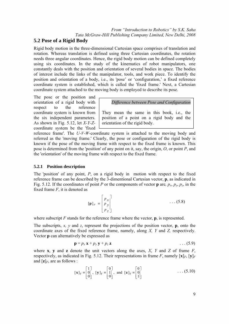
Difference between Pose and Configuration They mean the same in this book, i.e., the position of a point on a rigid body and the orientation of the rigid body.
5.2 Pose of a Rigid Body Rigid body motion in the three-dimensional Cartesian space comprises of translation and rotation. Whereas translation is defined using three Cartesian coordinates, the rotation needs three angular coordinates. Hence, the rigid body motion can be defined completely using six coordinates. In the study of the kinematics of robot manipulators, one constantly deals with the position and orientation of several bodies in space. The bodies of interest include the links of the manipulator, tools, and work piece. To identify the position and orientation of a body, i.e., its 'pose’ or ‘configuration,’ a fixed reference coordinate system is established, which is called the 'fixed frame.' Next, a Cartesian coordinate system attached to the moving body is employed to describe its pose.
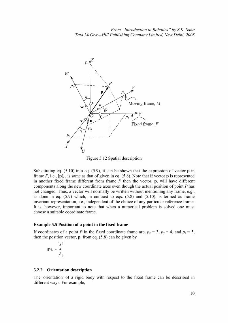
The pose or the position and orientation of a rigid body with respect to the reference coordinate system is known from the six independent parameters. As shown in Fig. 5.12, let X-Y-Z-coordinate system be the 'fixed reference frame'. The U-V-W-coordinate system is attached to the moving body and referred as the 'moving frame.' Clearly, the pose or configuration of the rigid body is known if the pose of the moving frame with respect to the fixed frame is known. This pose is determined from the 'position' of any point on it, say, the origin, O, or point P, and the 'orientation' of the moving frame with respect to the fixed frame.
5.2.1 Position description
The 'position' of any point, P, on a rigid body in motion with respect to the fixed reference frame can be described by the 3-dimentional Cartesian vector, p, as indicated in Fig. 5.12. If the coordinates of point P or the components of vector p are, px, py, pz, in the fixed frame F, it is denoted as
⎥⎥⎥
⎦
⎤
⎢⎢⎢
⎣
⎡
≡xp
zpypF][p . . . (5.8)
where subscript F stands for the reference frame where the vector, p, is represented.
The subscripts, x, y and z, represent the projections of the position vector, p, onto the coordinate axes of the fixed reference frame, namely, along X, Y and Z, respectively. Vector p can alternatively be expressed as
p = px x + py y + pz z . . . (5.9)
where x, y and z denote the unit vectors along the axes, X, Y and Z of frame F, respectively, as indicated in Fig. 5.12. Their representations in frame F, namely [x]F, [y]F and [z]F, are as follows :
⎥⎥⎦
⎤
⎢⎢⎣
⎡≡
⎥⎥⎦
⎤
⎢⎢⎣
⎡≡
⎥⎥⎦
⎤
⎢⎢⎣
⎡≡
0
10][and,
0
01][,
1
00][ FFF zyx . . . (5.10)
From “Introduction to Robotics” by S.K. Saha Tata McGraw-Hill Publishing Company Limited, New Delhi, 2008
10
Figure 5.12 Spatial description
Substituting eq. (5.10) into eq. (5.9), it can be shown that the expression of vector p in frame F, i.e., [p]F, is same as that of given in eq. (5.8). Note that if vector p is represented in another fixed frame different from frame F then the vector, p, will have different components along the new coordinate axes even though the actual position of point P has not changed. Thus, a vector will normally be written without mentioning any frame, e.g., as done in eq. (5.9) which, in contrast to eqs. (5.8) and (5.10), is termed as frame invariant representation, i.e., independent of the choice of any particular reference frame. It is, however, important to note that when a numerical problem is solved one must choose a suitable coordinate frame.
Example 5.5 Position of a point in the fixed frame
If coordinates of a point P in the fixed coordinate frame are, px = 3, py = 4, and pz = 5, then the position vector, p, from eq. (5.8) can be given by
⎥⎥⎥⎥
⎦
⎤
⎢⎢⎢⎢
⎣
⎡
≡
3
54F][p
5.2.2 Orientation description
The 'orientation' of a rigid body with respect to the fixed frame can be described in different ways. For example,
p
Fixed frame, Fpu
px
P
v
uy
x
zw
pw
O
U
py
W
X
Vpv
pz Z
Moving frame, M
Y
α
β
γ
From “Introduction to Robotics” by S.K. Saha Tata McGraw-Hill Publishing Company Limited, New Delhi, 2008
11
(i) Direction Cosine Representation;
(ii) Euler Angle Representation; and others.
Each one has its own limitations. If necessary, one may switch from one to other representation during a robot’s motion control to avoid former's limitations. Here, the above two will be presented which are sufficient to understand the underlying concepts and their limitations. Anybody interested in other representations may refer to the books by Tsai (1999) or Angeles (2003).
(i) Direction Cosine Representation
To describe the orientation or rotation of a rigid body, consider the motion of a moving frame M with respect to a fixed frame F, with one point fixed, say, the origin of the fixed frame, O, as shown in Fig. 5.12. Let u, v and w denote the three unit vectors pointing along the coordinates axes, U, V and W of the moving frame M, respectively, similar to the unit vectors, x, y, and z, along X, Y and Z of the fixed frame F, respectively. Since each of the unit vectors, u, v or w, denotes the position of a point at a unit distance from the origin on the axes of frame M, they are expressed using their projections on the X, Y, Z axes of the frame F as
u = ux x + uy y + uz z . . . (5.11a)
v = vx x + vy y + vz z . . . (5.11b)
w = wx x + wy y + wz z . . . (5.11c)
where ux, uy and uz are the components of the unit vector, u, along X, Y and Z axes, respectively. Similarly vx, vy, vz, and wx, wy, wz are defined for the unit vectors, v and w, respectively. Now, point P of the rigid body, as shown in Fig. 5.12 and given by eq. (5.8), is expressed in the moving frame, M, as
p = puu + pvv + pww . . . (5.12)
where pu, pv, and pw are the components of the vector, p, along U, V, W axes of the moving frame, M. Upon substitution of eqs. (5.11a-c) into eq. (5.12) yields
p = (puux + pvvx + pwwx)x + (puuy + pvvy + pwwy)y + (puuz + pvvz + pwwz)z . . . (5.13)
Comparing the right hand sides of eqs. (5.8) and (5.13), the following identities are obtained:
px = uxpu + vxpv + wxpw . . . (5.14a)
py = uypu + vypv + wypw . . . (5.14b)
pz = uzpu + vzpv + wzpw . . . (5.14c)
Equations (5.14a-c) are written in a matrix form as
[p]F = Q [p]M . . . (5.15)
where [p]F and [p]M are the representations of the 3-dimensional vector, p, in frames F and M, respectively, and Q is the 3 × 3 rotation or orientation matrix transforming the representation of vector p from frame M to F. They are given as follows:
From “Introduction to Robotics” by S.K. Saha Tata McGraw-Hill Publishing Company Limited, New Delhi, 2008
12
⎥⎥⎥⎥
⎦
⎤
⎢⎢⎢⎢
⎣
⎡
=
⎥⎥⎥⎥
⎦
⎤
⎢⎢⎢⎢
⎣
⎡
≡⎥⎥⎥
⎦
⎤
⎢⎢⎢
⎣
⎡≡
⎥⎥⎥⎥
⎦
⎤
⎢⎢⎢⎢
⎣
⎡
≡
xTwxTvxTu
zTwzTvzTuyTwyTvyTuQpp
xwxvxu
zwzvzuywyvyu
up
wpvp
xp
zpyp MF and,][,][ . . . (5.16)
Note the columns of matrix Q. They are nothing but the components of the orthogonal (meaning 90o to each other) unit vectors, u, v, and w in the fixed frame F, which must satisfy the following six orthogonal conditions:
uTu = vTv = wTw = 1, and uTv(≡vTu) = uTw(≡wTu) = vTw(≡wTv) = 0 . . . (5.17)
Moreover, for the three orthogonal vectors, u, v and w, the following hold true:
u × v = w, v × w = u, and w × u = v . . . (5.18)
Hence, the 3 × 3 'rotation matrix,' Q, denoting the orientation of the moving frame, M, with respect to the fixed frame, F, is called 'orthogonal.' It satisfies the following properties due to eq. (5.17):
QTQ = QQT = 1 ; where det (Q) = 1, and Q−1 = QT . . . (5.19)
1 being the 3 × 3 identity matrix. Moreover, if one is interested to find the rotation description of the frame, F, with respect to frame M denoted by Q’, it can be derived similarly. It can be shown that Q’ = QT.
Also note from eq. (5.16), that the (1,1) element of Q is the cosine of the angle between the vectors u and x, i.e., uTx. The same holds true with other elements of Q. Hence, this rotation matrix is known as the 'Direction Cosine Representation' of the rotation matrix. Such representation requires nine parameters, namely, the elements of the 3 × 3 matrix, Q. However, not all the nine parameters are independent as they must satisfy the six conditions of eq. (5.17). Thus, only three parameters are independent and should be sufficient to define the three-DOF rotational motion. It is, however, difficult to choose the set of three independent parameters. This is the drawback of the Direction Cosine Representation.
Example 5.6 Elementary Rotations
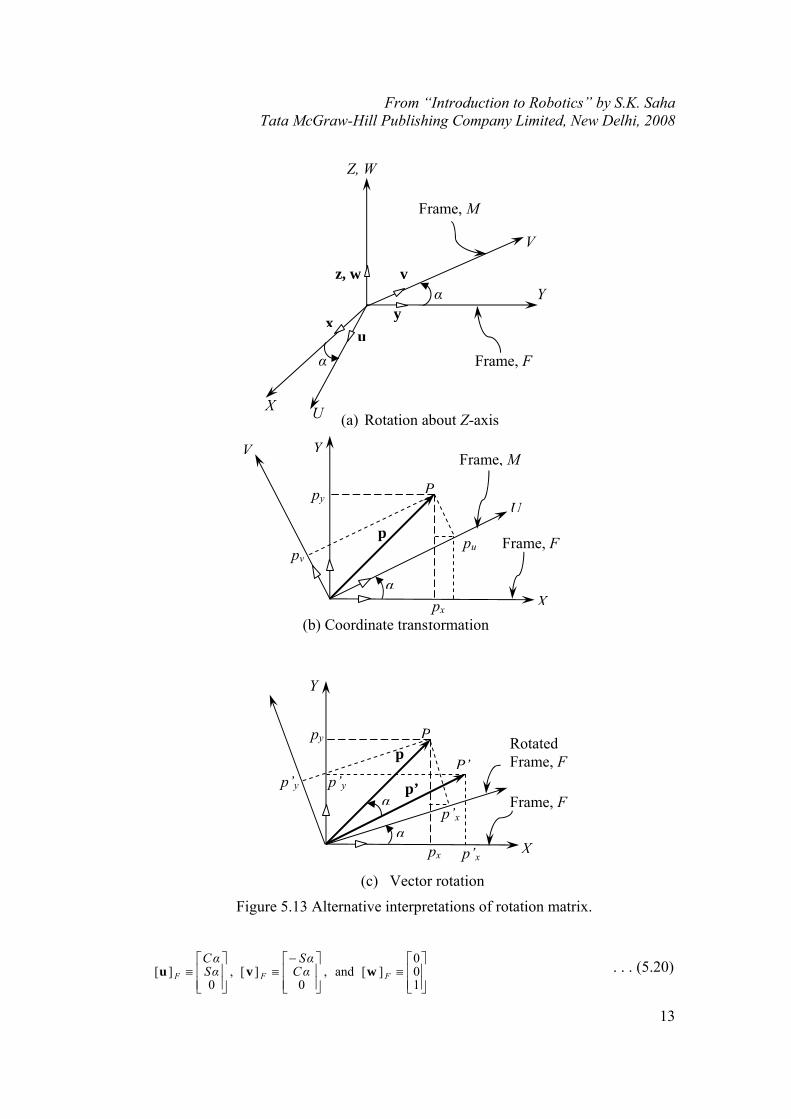
Suppose that a reference frame M coincides with the fixed frame F. Now, frame M is rotated by an angle α about the axis Z, as shown in Fig. 5.13(a). The unit vectors of the new frame M can be described in terms of their components in the reference frame, F, as
From “Introduction to Robotics” by S.K. Saha Tata McGraw-Hill Publishing Company Limited, New Delhi, 2008
13
(a) Rotation about Z-axis
(b) Coordinate transformation
(c) Vector rotation
Figure 5.13 Alternative interpretations of rotation matrix.
⎥⎥⎦
⎤
⎢⎢⎣
⎡≡
⎥⎥⎦
⎤
⎢⎢⎣
⎡−≡
⎥⎥⎦
⎤
⎢⎢⎣
⎡≡
0
10][and,
0][,
0][ FFF
SαCα
CαSα wvu . . . (5.20)
z, w
y x
v
α
α
Z, W
X
u
Y
V
Frame, M
Frame, F
U
p
Y
pu
Xα
px
pv
py
Frame, F
U
Frame, M
P
V
p
p’y
p’x
Y
X
α
px
py
Frame, F
P
P’p’
p’x
p’y
α
Rotated Frame, F
From “Introduction to Robotics” by S.K. Saha Tata McGraw-Hill Publishing Company Limited, New Delhi, 2008
14
where, S≡sin; C≡cos. Hence, the rotation matrix denoted by QZ is given by
⎥⎥⎥
⎦
⎤
⎢⎢⎢
⎣
⎡ααα−α
≡10000
CSSC
ZQ . . . (5.21)
In a similar manner, it can be shown that the rotations of angle β about axis Y, and by an angle γ about axis X are, respectively, given by
⎥⎥⎥
⎦
⎤
⎢⎢⎢
⎣
⎡−≡
⎥⎥⎥
⎦
⎤
⎢⎢⎢
⎣
⎡
−≡
γγγγ
ββ
ββ
CSSC
CS
SC
XY
00
001and,
0010
0QQ . . . (5.22)
The above matrices in eqs. (5.21) and (5.22) are called the 'elementary rotations' and are useful to describe any arbitrary rotation while the angles with respect to the coordinate axes are known.
Example 5.7 Properties of Elementary Rotation Matrices
From eqs. (5.21) and (5.22), matrix multiplication of, say, QzT and Qz results the
following:
⎥⎥⎥
⎦
⎤
⎢⎢⎢
⎣
⎡=
⎥⎥⎥
⎦
⎤
⎢⎢⎢
⎣
⎡ααα−α
⎥⎥⎥
⎦
⎤
⎢⎢⎢
⎣
⎡αα−αα
=100010001
10000
10000
CSSC
CSSC
zTz QQ
Using the definition of determinant given in Appendix A, it can be easily calculated that det(Qz)=1. Hence, Qz satisfies both the properties of a rotation matrix. Similarly, the other two matrices can be shown to have the properties of a rotation matrix as well.
Example 5.8 Coordinate Transformation
Consider two coordinate frames with a common origin. One of them is rotated by an angle α about the axis Z. Let [p]F and [p]M be the vector representations of point P in frames F and M, respectively, as shown in Fig. 5.13(b). On the basis of simple geometry, the relationships between the coordinates of point P in the two coordinate frames are given by
px = pu Cα − pv Sα . . . (5.23)
py = pu Sα + pv Cα . . . (5.24)
pz = pw . . . (5.25)
where px, py, pz , and pu, pv, pw are the three coordinates of point P along the axes of frames F and M, respectively. It is easy to recognize from eqs. (5.23) to (5.25) that the vector [p]F ≡ [px, py, pz]T is nothing but
[p]F =QZ [p]M . . . (5.26)
where [p]M ≡ [pu, pv, pw]T and QZ is given by eq. (5.21). Matrix QZ not only represents the orientation of the frame, M, with respect to the fixed frame, F, as in Fig. 5.13(a), but
From “Introduction to Robotics” by S.K. Saha Tata McGraw-Hill Publishing Company Limited, New Delhi, 2008
15
also transforms the representation of a vector from frame M, say, [p]M, to another frame F with the same origin, i.e., [p]F.
Example 5.9 Vector Rotation
Consider the vector, p, which is obtained by rotating a vector p′ in the X-Y-plane by an angle α about the axis, Z, of the reference frame, F of Fig. 5.13(c). Let p′x, p′y, p′z be the coordinates of vector p′ in frame F, i.e., [p′]F ≡ [p′x, p′y, p′z]T. Then, vector p in frame F, [p]F, has the following components.
px = p′x Cα − p′y Sα . . . (5.27)
py = p′x Sα + p′y Cα . . . (5.28)
pz = p′z . . . (5.29)
which can be obtained by rotating the fixed frame, F, with which vector p’ is attached by an angle α counter clockwise about the Z-axis so that vector p’ reaches p, as indicated in Fig. 5.13(c). Equations (5.27)-(5.29) can be written in compact form as
[p]F = QZ [p′]F . . . (5.30)
where QZ is given by eq. (5.21).
(ii) Euler Angles Representation
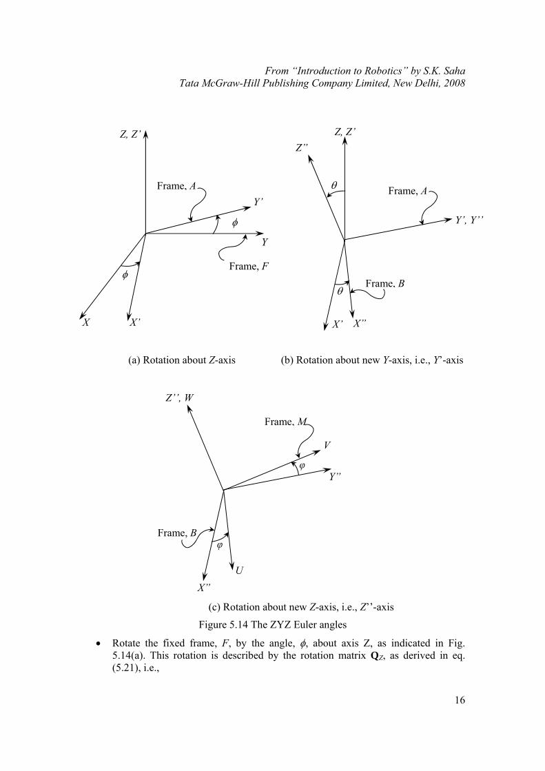
The Euler angles constitute a 'minimal' representation of orientation obtained by composing three elementary rotations with respect to the axes of current frames. There is a possibility of twelve distinct sets of Euler angles with regard to the sequence of possible elementary rotations, namely, XYZ, XZY, XZX, XYX, YXZ, YZX, YXY, YZY, ZXY, ZYZ, ZXZ, and ZYZ. Amongst all, the ZYZ set is commonly used in the Euler angles representation. This implies that the fixed frame, F, first rotates about its Z-axis to reach an intermediate frame A, then about Y-axis of the rotated frame, i.e., Y’ of frame A, to reach another intermediate frame B, and, finally, about Z-axis of the twice rotated frame, i.e., Z’’ of frame B, to reach the desired frame M, as shown in Fig. 5.14. Let φ, θ, and ϕ be the angles about Z, Y’, and Z’’, respectively. The overall rotation described by these angles is then obtained as the composition of elementary rotations, as explained below: Referring to Fig. 5.14,
From “Introduction to Robotics” by S.K. Saha Tata McGraw-Hill Publishing Company Limited, New Delhi, 2008
16
(a) Rotation about Z-axis (b) Rotation about new Y-axis, i.e., Y’-axis
(c) Rotation about new Z-axis, i.e., Z’’-axis
Figure 5.14 The ZYZ Euler angles
• Rotate the fixed frame, F, by the angle, φ, about axis Z, as indicated in Fig. 5.14(a). This rotation is described by the rotation matrix QZ, as derived in eq. (5.21), i.e.,
Frame, F
Frame, A
X’ X
Y
Y’
Z, Z’
φ
φ
Frame, B
Frame, M
U
Z’’, W
V
Y”
X”
φ
φ
Frame, A
Frame, B
Z”Z, Z’
Y’, Y’’
X’
θ
θ
X”
From “Introduction to Robotics” by S.K. Saha Tata McGraw-Hill Publishing Company Limited, New Delhi, 2008
17
⎥⎥⎥
⎦
⎤
⎢⎢⎢
⎣
⎡φφφ−φ
≡1000CS0SC
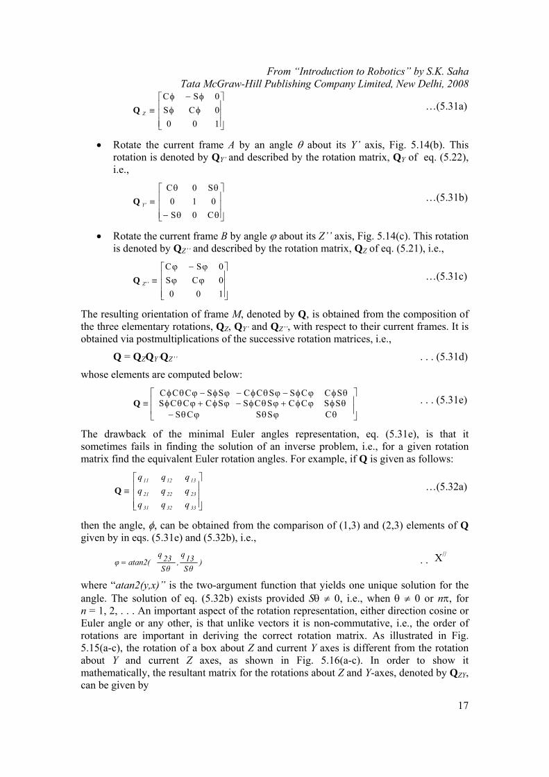
ZQ …(5.31a)
• Rotate the current frame A by an angle θ about its Y’ axis, Fig. 5.14(b). This rotation is denoted by QY’ and described by the rotation matrix, QY of eq. (5.22), i.e.,
⎥⎥⎥
⎦
⎤
⎢⎢⎢
⎣
⎡
θθ−
θθ≡
C0S010
S0C
Y'Q …(5.31b)
• Rotate the current frame B by angle ϕ about its Z’’ axis, Fig. 5.14(c). This rotation is denoted by QZ’’ and described by the rotation matrix, QZ of eq. (5.21), i.e.,
⎥⎥⎥
⎦
⎤
⎢⎢⎢
⎣
⎡ϕϕϕ−ϕ
≡1000CS0SC
'Z'Q …(5.31c)
The resulting orientation of frame M, denoted by Q, is obtained from the composition of the three elementary rotations, QZ, QY’ and QZ’’, with respect to their current frames. It is obtained via postmultiplications of the successive rotation matrices, i.e.,
Q = QZQY’QZ’’ . . . (5.31d)
whose elements are computed below:
⎥⎥
⎦
⎤
⎢⎢
⎣
⎡ θφϕφ−ϕθφ−ϕφ−ϕθφ
θϕθϕθ−θφϕφ+ϕθφ−ϕφ+ϕθφ≡
SCCSSCCSSCCC
CSSCSSSCCSCSSCCCSQ . . . (5.31e)
The drawback of the minimal Euler angles representation, eq. (5.31e), is that it sometimes fails in finding the solution of an inverse problem, i.e., for a given rotation matrix find the equivalent Euler rotation angles. For example, if Q is given as follows:
⎥⎥⎥
⎦
⎤
⎢⎢⎢
⎣
⎡≡
333231
232221
131211
qqqqqqqqq
Q …(5.32a)
then the angle, φ, can be obtained from the comparison of (1,3) and (2,3) elements of Q given by in eqs. (5.31e) and (5.32b), i.e.,
)Sθ13q
,Sθ23q
atan2(φ = . . . (5.32b)
where “atan2(y,x)” is the two-argument function that yields one unique solution for the angle. The solution of eq. (5.32b) exists provided Sθ ≠ 0, i.e., when θ ≠ 0 or nπ, for n = 1, 2, . . . An important aspect of the rotation representation, either direction cosine or Euler angle or any other, is that unlike vectors it is non-commutative, i.e., the order of rotations are important in deriving the correct rotation matrix. As illustrated in Fig. 5.15(a-c), the rotation of a box about Z and current Y axes is different from the rotation about Y and current Z axes, as shown in Fig. 5.16(a-c). In order to show it mathematically, the resultant matrix for the rotations about Z and Y-axes, denoted by QZY, can be given by
X//
From “Introduction to Robotics” by S.K. Saha Tata McGraw-Hill Publishing Company Limited, New Delhi, 2008
18
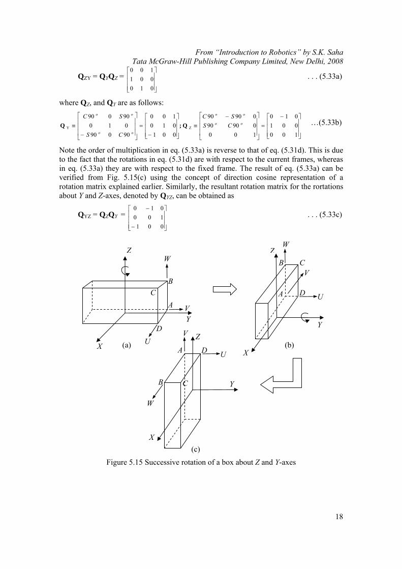
QZY = QYQZ = ⎥⎥⎥
⎦
⎤
⎢⎢⎢
⎣
⎡
010001100
. . . (5.33a)
where QZ, and QY are as follows:
⎥⎥⎥
⎦
⎤
⎢⎢⎢
⎣
⎡ −=
⎥⎥⎥
⎦
⎤
⎢⎢⎢
⎣
⎡ −≡
⎥⎥⎥
⎦
⎤
⎢⎢⎢
⎣
⎡
−=
⎥⎥⎥
⎦
⎤
⎢⎢⎢
⎣
⎡
−≡
100001010
1000909009090
001010100
90090010
90090
ZYoo
oo
oo
oo
CSSC
CS
SCQ ;Q …(5.33b)
Note the order of multiplication in eq. (5.33a) is reverse to that of eq. (5.31d). This is due to the fact that the rotations in eq. (5.31d) are with respect to the current frames, whereas in eq. (5.33a) they are with respect to the fixed frame. The result of eq. (5.33a) can be verified from Fig. 5.15(c) using the concept of direction cosine representation of a rotation matrix explained earlier. Similarly, the resultant rotation matrix for the rortations about Y and Z-axes, denoted by QYZ, can be obtained as
QYZ = QZQY = ⎥⎥⎥
⎦
⎤
⎢⎢⎢
⎣
⎡
−
−
001100010
. . . (5.33c)
(a) (b)
(c)
Figure 5.15 Successive rotation of a box about Z and Y-axes
X
Z
Y
A
B C
D U
V
W
Z
Y
X
A
B C
D U
V
W
X
Z
Y
A C
B
D U
W
V
From “Introduction to Robotics” by S.K. Saha Tata McGraw-Hill Publishing Company Limited, New Delhi, 2008
19
(a) (b)
(c)
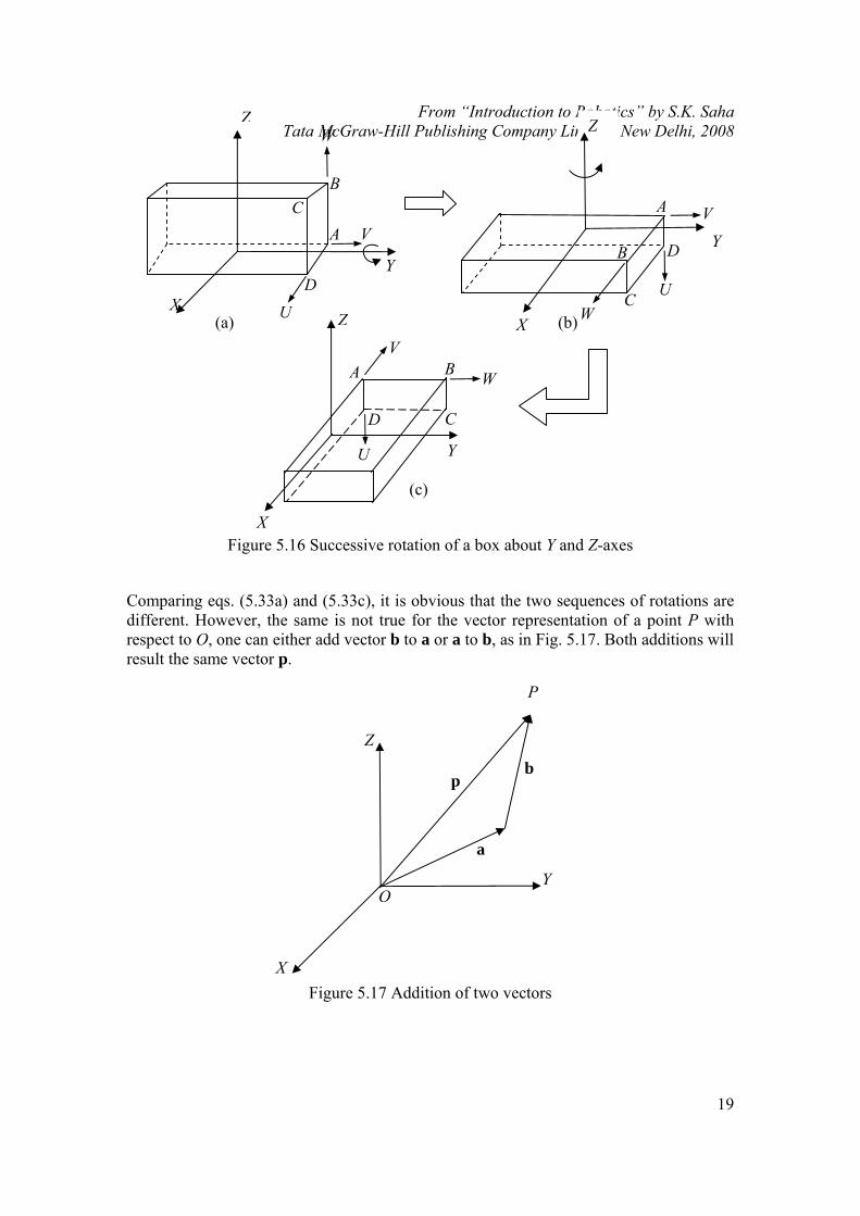
Figure 5.16 Successive rotation of a box about Y and Z-axes
Comparing eqs. (5.33a) and (5.33c), it is obvious that the two sequences of rotations are different. However, the same is not true for the vector representation of a point P with respect to O, one can either add vector b to a or a to b, as in Fig. 5.17. Both additions will result the same vector p.
Figure 5.17 Addition of two vectors
O
b
a
p
P
Y
Z
X
X
X
Y
Z
A B
CD
U
V
W
Z
Y
A C
B
D U
W
V
Z
X
Y
A
B
C
D
V
U W
From “Introduction to Robotics” by S.K. Saha Tata McGraw-Hill Publishing Company Limited, New Delhi, 2008
20
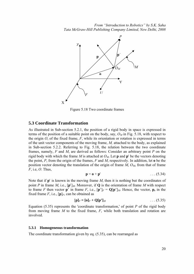
Figure 5.18 Two coordinate frames
5.3 Coordinate Transformation As illustrated in Sub-section 5.2.1, the position of a rigid body in space is expressed in terms of the position of a suitable point on the body, say, OM in Fig. 5.18, with respect to the origin O, of the fixed frame, F, while its orientation or rotation is expressed in terms of the unit vector components of the moving frame, M, attached to the body, as explained in Sub-section 5.2.2. Referring to Fig. 5.18, the relation between the two coordinate frames, namely, F and M, are derived as follows: Consider an arbitrary point P on the rigid body with which the frame M is attached at OM. Let p and p′ be the vectors denoting the point, P, from the origin of the frames, F and M, respectively. In addition, let o be the position vector denoting the translation of the origin of frame M, OM, from that of frame F, i.e, O. Thus,
p = o + p′ . . . (5.34)
Note that if p′ is known in the moving frame M, then it is nothing but the coordinates of point P in frame M, i.e., [p′]M. Moreover, if Q is the orientation of frame M with respect to frame F then vector p’ in frame F, i.e., [p’]F = Q[p’]M. Hence, the vector, p, in the fixed frame F, i.e., [p]F, can be obtained as
[p]F = [o]F + Q[p’]M . . . (5.35)
Equation (5.35) represents the 'coordinate transformation,' of point P of the rigid body from moving frame M to the fixed frame, F, while both translation and rotation are involved.
5.3.1 Homogeneous transformation
The coordinate transformation given by eq. (5.35), can be rearranged as
F
p΄
o
p
U
M OM
P
X
Z
Y
From “Introduction to Robotics” by S.K. Saha Tata McGraw-Hill Publishing Company Limited, New Delhi, 2008
21
Why Homogenous? Matrix T of eq. (5.36) takes care of both the translation and rotation of the frame attached to the body with respect to the fixed frame.
⎥⎦
⎤⎢⎣
⎡ ′⎥⎦
⎤⎢⎣
⎡=⎥
⎦
⎤⎢⎣
⎡1][
1][
1][
TF MF poQp
0 . . . (5.36)
where 0 ≡ [0, 0, 0]T is the three-dimensional vector of zeros. Equation (5.36) is written in a compact form as
MF ][][ pTp ′= . . . (5.37)
where MF ][and][ pp ′ are the four-dimensional vectors obtained by putting one at the bottom of the original three-dimensional vectors, [p]F and [p’]M, respectively, as the fourth element, whereas the 4 × 4 matrix, T, is called 'homogeneous transformation matrix.' Equation (5.37) is simple in a sense that the transformation of a vector, which includes both translation and rotation from frame M to F, is done by just multiplying one
4 × 4 matrix, instead of a matrix multiplication and vector addition, as in eq. (5.35). However, from the view of computational complexity, i.e., the numbers of multiplications/divisions and additions/subtractions required in a computer program, eq. (5.35) is economical compared to eq. (5.36) or (5.37), as some unnecessary multiplications and additions with 1s and 0s will
be performed. It is pointed out here that, for the homogeneous transformation matrix, T, the orthogonality property does not hold good, i.e.,
TTT ≠ 1 or T−1 ≠ TT . . . (5.38)
However, the inverse of the homogeneous transformations matrix, T, can be obtained easily from eq. (5.36) as
⎥⎥⎦
⎤
⎢⎢⎣
⎡ −=−
1][
T
TT1
0oQQT F . . . (5.39)
(a) (b)
2 1
W
M
F U
V
Z
Y
X
30˚
30˚
U
Z, W
F
X
Y
VM
From “Introduction to Robotics” by S.K. Saha Tata McGraw-Hill Publishing Company Limited, New Delhi, 2008
22
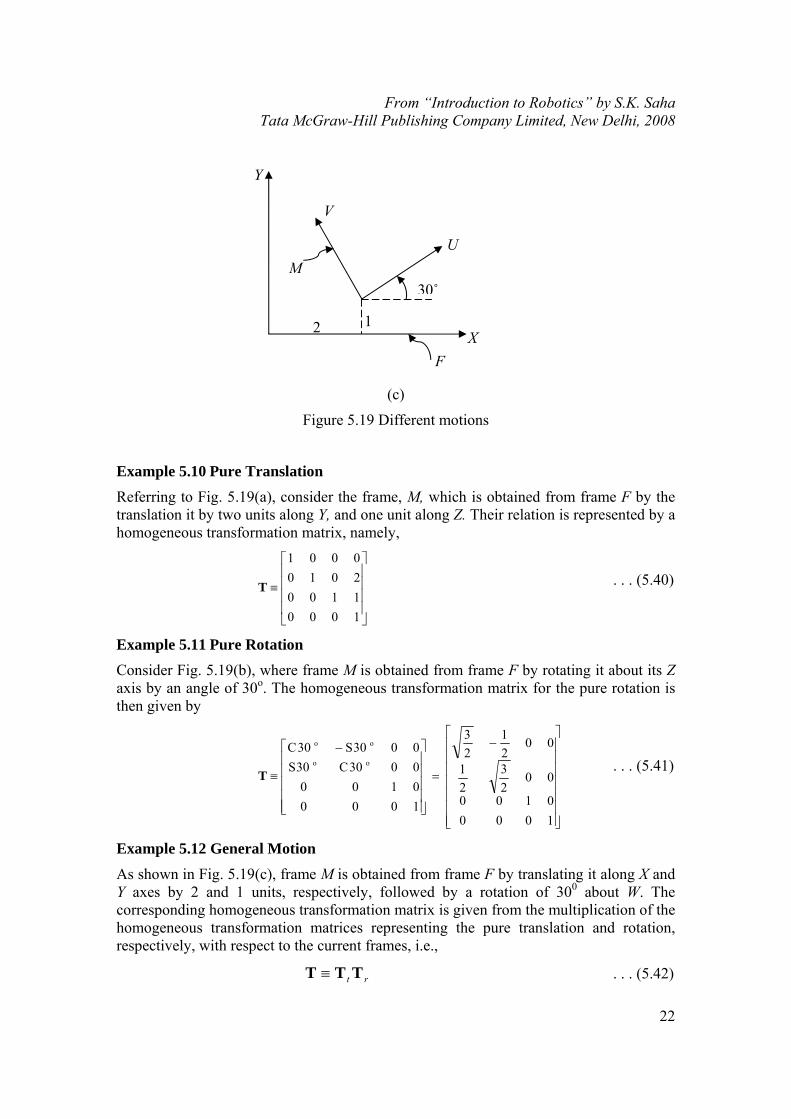
(c)
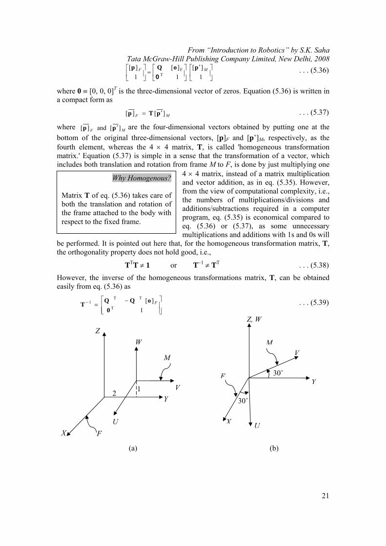
Figure 5.19 Different motions
Example 5.10 Pure Translation
Referring to Fig. 5.19(a), consider the frame, M, which is obtained from frame F by the translation it by two units along Y, and one unit along Z. Their relation is represented by a homogeneous transformation matrix, namely,
⎥⎥⎥⎥
⎦
⎤
⎢⎢⎢⎢
⎣
⎡
≡
1000110020100001
T . . . (5.40)
Example 5.11 Pure Rotation
Consider Fig. 5.19(b), where frame M is obtained from frame F by rotating it about its Z axis by an angle of 30o. The homogeneous transformation matrix for the pure rotation is then given by
⎥⎥⎥⎥⎥⎥⎥
⎦
⎤
⎢⎢⎢⎢⎢⎢⎢
⎣
⎡−
=
⎥⎥⎥⎥⎥
⎦
⎤
⎢⎢⎢⎢⎢
⎣
⎡ −
≡
10000100
0023
21
0021
23
100001000030C30S0030S30C
oo
oo
T . . . (5.41)
Example 5.12 General Motion
As shown in Fig. 5.19(c), frame M is obtained from frame F by translating it along X and Y axes by 2 and 1 units, respectively, followed by a rotation of 300 about W. The corresponding homogeneous transformation matrix is given from the multiplication of the homogeneous transformation matrices representing the pure translation and rotation, respectively, with respect to the current frames, i.e.,
rt TTT ≡ . . . (5.42)
2 1
30˚
U
V
X
Y
M
F
From “Introduction to Robotics” by S.K. Saha Tata McGraw-Hill Publishing Company Limited, New Delhi, 2008
23
where subscripts 't' and 'r' stand for ‘translation’ and 'rotation', respectively, whereas Tt and Tt are given by eqs. (5.40) and (5.41), respectively. The resultant matrix, T, is given by
⎥⎥⎥⎥⎥⎥⎥
⎦
⎤
⎢⎢⎢⎢⎢⎢⎢
⎣
⎡−
=
⎥⎥⎥⎥⎥
⎦
⎤
⎢⎢⎢⎢⎢
⎣
⎡ −
≡
10000100
1023
21
2021
23
100001001030C30S2030S30C
oo
oo
T . . . (5.43)
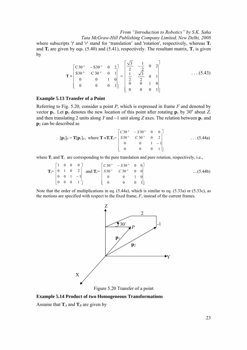
Example 5.13 Transfer of a Point
Referring to Fig. 5.20, consider a point P, which is expressed in frame F and denoted by vector p1. Let p2 denotes the new location of this point after rotating p1 by 30o about Z, and then translating 2 units along Y and −1 unit along Z axes. The relation between p1 and p2 can be described as
[p2]F = T[p1]F, where T ≡TtTr=
⎥⎥⎥⎥⎥
⎦
⎤
⎢⎢⎢⎢⎢
⎣
⎡
−
−
10001100
203030003030
oo
oo
CSSC
. . . (5.44a)
where Tt and Tr are corresponding to the pure translation and pure rotation, respectively, i.e.,
Tt=
⎥⎥⎥⎥
⎦
⎤
⎢⎢⎢⎢
⎣
⎡
−10001100
20100001
and Tr=
⎥⎥⎥⎥⎥
⎦
⎤
⎢⎢⎢⎢⎢
⎣
⎡ −
10000100003030003030
oo
oo
CSSC
…(5.44b)
Note that the order of multiplications in eq. (5.44a), which is similar to eq. (5.33a) or (5.33c), as the motions are specified with respect to the fixed frame, F, instead of the current frames.
Figure 5.20 Transfer of a point
Example 5.14 Product of two Homogeneous Transformations
Assume that TA and TB are given by
2
-130˚
p1
p2
Y
Z
X
P
From “Introduction to Robotics” by S.K. Saha Tata McGraw-Hill Publishing Company Limited, New Delhi, 2008
24
⎥⎥⎥⎥⎥
⎦
⎤
⎢⎢⎢⎢⎢
⎣
⎡ −
=
10000100103030203030
oo
oo
ACS
SC
T , and
⎥⎥⎥⎥⎥
⎦
⎤
⎢⎢⎢⎢⎢
⎣
⎡
−=
10000100104545104545
oo
oo
BCSSC
T . . . (5.45)
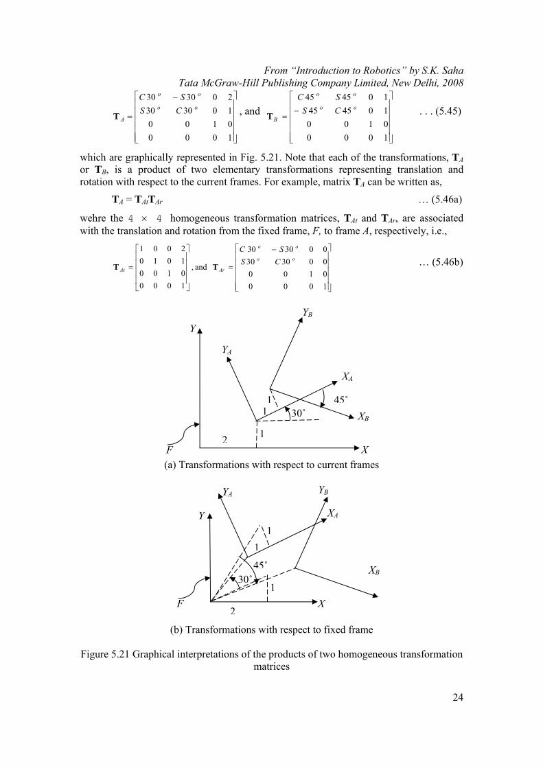
which are graphically represented in Fig. 5.21. Note that each of the transformations, TA or TB, is a product of two elementary transformations representing translation and rotation with respect to the current frames. For example, matrix TA can be written as,
TA = TAtTAr … (5.46a)
wehre the 4 × 4 homogeneous transformation matrices, TAt and TAr, are associated with the translation and rotation from the fixed frame, F, to frame A, respectively, i.e.,
⎥⎥⎥⎥⎥
⎦
⎤
⎢⎢⎢⎢⎢
⎣
⎡ −
=
⎥⎥⎥⎥
⎦
⎤
⎢⎢⎢⎢
⎣
⎡
=
10000100003030003030
and,
1000010010102001
oo
oo
ArAtCS
SC
TT … (5.46b)
(a) Transformations with respect to current frames
(b) Transformations with respect to fixed frame
Figure 5.21 Graphical interpretations of the products of two homogeneous transformation matrices
F
XA
30˚45˚
X
YA
XB
YB
Y
1
2
11
F
XA
30˚45˚
X
YA
XB
YB
Y
12
11
From “Introduction to Robotics” by S.K. Saha Tata McGraw-Hill Publishing Company Limited, New Delhi, 2008
25
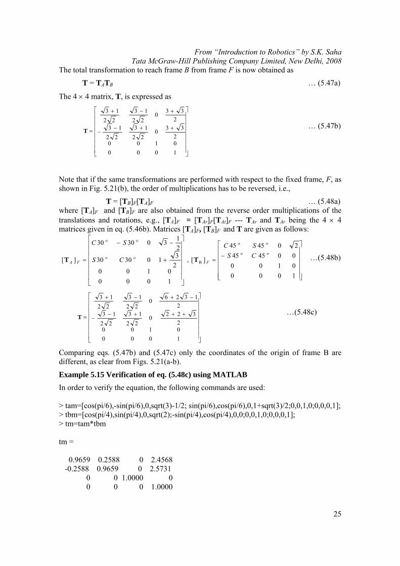
The total transformation to reach frame B from frame F is now obtained as
T = TATB … (5.47a)
The 4 × 4 matrix, T, is expressed as
⎥⎥⎥⎥⎥⎥⎥
⎦
⎤
⎢⎢⎢⎢⎢⎢⎢
⎣
⎡
++−−
+−+
=
100001002
33022
1322
132
33022
1322
13
T … (5.47b)
Note that if the same transformations are performed with respect to the fixed frame, F, as shown in Fig. 5.21(b), the order of multiplications has to be reversed, i.e.,
T = [TB]F[TA]F … (5.48a) where [TA]F and [TB]F are also obtained from the reverse order multiplications of the translations and rotations, e.g., [TA]F = [TAr]F[TAt]F --- TAr and TAr being the 4 × 4 matrices given in eq. (5.46b). Matrices [TA]F, [TB]F and T are given as follows:
⎥⎥⎥⎥⎥
⎦
⎤
⎢⎢⎢⎢⎢
⎣
⎡
−=
⎥⎥⎥⎥⎥⎥
⎦
⎤
⎢⎢⎢⎢⎢⎢
⎣
⎡
+
−−
=
10000100004545204545
][,
10000100
23103030
21303030
][ B
oo
oo
Foo
oo
FACSSC
CS
SC
TT …(5.48b)
⎥⎥⎥⎥⎥⎥⎥
⎦
⎤
⎢⎢⎢⎢⎢⎢⎢
⎣
⎡
+++−−
−+−+
=
100001002
322022
1322
132
1326022
1322
13
T …(5.48c)
Comparing eqs. (5.47b) and (5.47c) only the coordinates of the origin of frame B are different, as clear from Figs. 5.21(a-b).
Example 5.15 Verification of eq. (5.48c) using MATLAB
In order to verify the equation, the following commands are used: > tam=[cos(pi/6),-sin(pi/6),0,sqrt(3)-1/2; sin(pi/6),cos(pi/6),0,1+sqrt(3)/2;0,0,1,0;0,0,0,1]; > tbm=[cos(pi/4),sin(pi/4),0,sqrt(2);-sin(pi/4),cos(pi/4),0,0;0,0,1,0;0,0,0,1]; > tm=tam*tbm tm = 0.9659 0.2588 0 2.4568 -0.2588 0.9659 0 2.5731 0 0 1.0000 0 0 0 0 1.0000
From “Introduction to Robotics” by S.K. Saha Tata McGraw-Hill Publishing Company Limited, New Delhi, 2008
26
First appearance of DH parameters The DH parameters were first appeared in 1955 (Denavit and Hartenberg, 1955) to represent a directed line which is nothing but the axis of a lower pair joint.
where ‘tam’ and ‘tbm’ represent the matrices, [TA]F and [TB]F , respectively, whereas the resultant matrix, [TA]F , is denoted by ‘tm.’ Equation (5.48c) can be easily verified to be the expression given by ‘tm.’
5.4 Denvit and Hartenberg (DH) Parameters
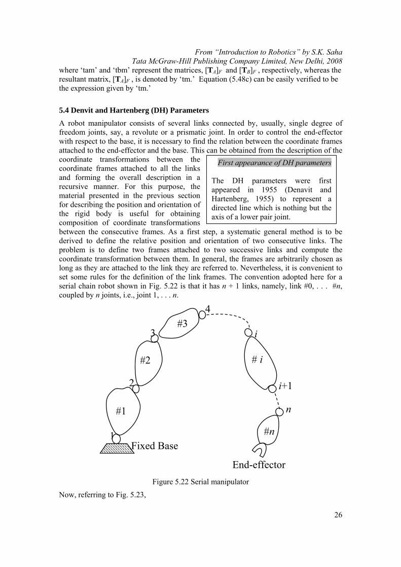
A robot manipulator consists of several links connected by, usually, single degree of freedom joints, say, a revolute or a prismatic joint. In order to control the end-effector with respect to the base, it is necessary to find the relation between the coordinate frames attached to the end-effector and the base. This can be obtained from the description of the coordinate transformations between the coordinate frames attached to all the links and forming the overall description in a recursive manner. For this purpose, the material presented in the previous section for describing the position and orientation of the rigid body is useful for obtaining composition of coordinate transformations between the consecutive frames. As a first step, a systematic general method is to be derived to define the relative position and orientation of two consecutive links. The problem is to define two frames attached to two successive links and compute the coordinate transformation between them. In general, the frames are arbitrarily chosen as long as they are attached to the link they are referred to. Nevertheless, it is convenient to set some rules for the definition of the link frames. The convention adopted here for a serial chain robot shown in Fig. 5.22 is that it has n + 1 links, namely, link #0, . . . #n, coupled by n joints, i.e., joint 1, . . . n.
Figure 5.22 Serial manipulator
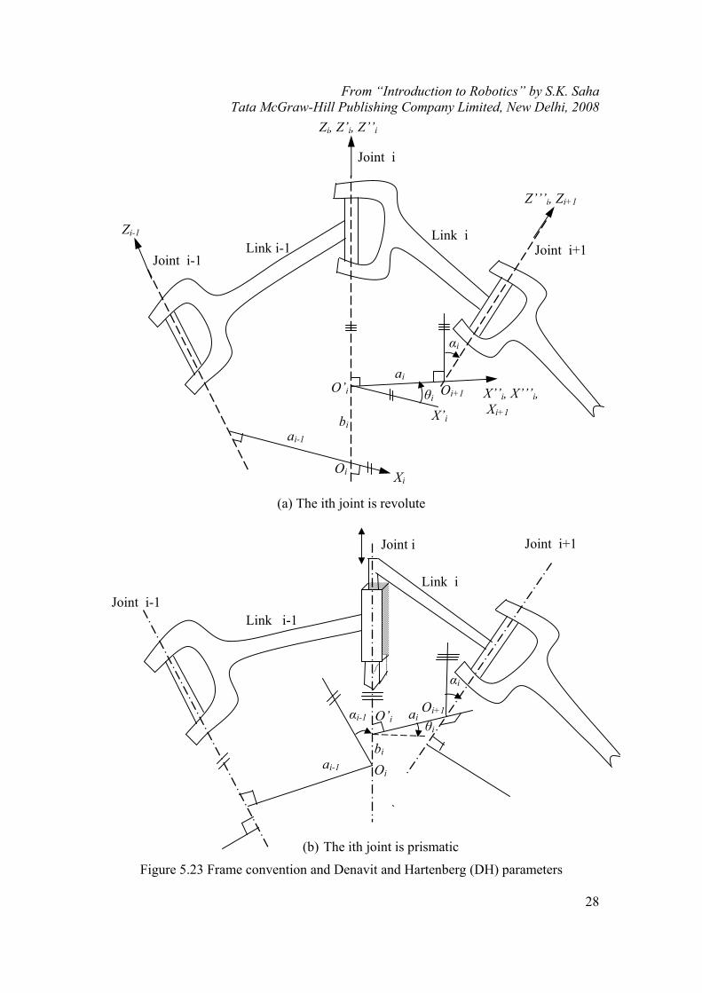
Now, referring to Fig. 5.23,
1 Fixed Base
i+1
#1
#2 # i
#n
2
3
4
i
n
#3
End-effector
From “Introduction to Robotics” by S.K. Saha Tata McGraw-Hill Publishing Company Limited, New Delhi, 2008
27
(a) Let axis i denotes the axis of the joint connecting link i −1 to link i.
(b) A coordinate system Xi, Yi, Zi is attached to the end of the link i −1 ⎯ not to the link i! ⎯ for i = 1, . . . n+1.
(c) Choose axis Zi along the axis of joint i, whose positive direction can be taken towards either direction of the axis.
(d) Locate the origin, Oi, at the intersection of axis Zi with the common normal to Zi − 1 and Zi. Also, locate O′i on Zi at the intersection of the common normal to Zi and Zi + 1.
(e) Choose axis Xi along the common normal to axes Zi − 1 and Zi with the direction from former to the later.
(f) Choose axis Yi so as to complete a right handed frame.
Note that the above conventions do not give a unique definition of the link frames in the following cases:
• For frame 1 that is attached to the fixed base, i.e., link 0, only the direction of axes Z1 is specified. Then O1 and X1 can be chosen arbitarily.
From “Introduction to Robotics” by S.K. Saha Tata McGraw-Hill Publishing Company Limited, New Delhi, 2008
28
(a) The ith joint is revolute
(b) The ith joint is prismatic
Figure 5.23 Frame convention and Denavit and Hartenberg (DH) parameters
αi
bi
θi
ai
ai-1
Joint i+1 Link i
Joint i-1 Link i-1
Xi
X’i
X’’i, X’’’i, Xi+1
Zi, Z’i, Z’’i
Joint i
Z’’’i, Zi+1
Zi-1
O’i
Oi
Oi+1
Joint i-1
αi-1
ai-1
αi
θi
Joint i+1 Joint i
Link i
Link i-1
Oi
O’i
bi
ai Oi+1
From “Introduction to Robotics” by S.K. Saha Tata McGraw-Hill Publishing Company Limited, New Delhi, 2008
29
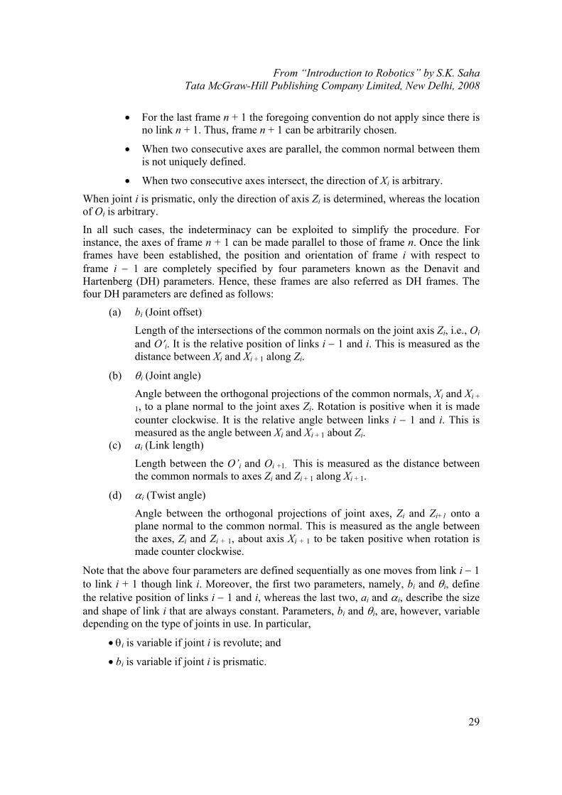
• For the last frame n + 1 the foregoing convention do not apply since there is no link n + 1. Thus, frame n + 1 can be arbitrarily chosen.
• When two consecutive axes are parallel, the common normal between them is not uniquely defined.
• When two consecutive axes intersect, the direction of Xi is arbitrary.
When joint i is prismatic, only the direction of axis Zi is determined, whereas the location of Oi is arbitrary.
In all such cases, the indeterminacy can be exploited to simplify the procedure. For instance, the axes of frame n + 1 can be made parallel to those of frame n. Once the link frames have been established, the position and orientation of frame i with respect to frame i − 1 are completely specified by four parameters known as the Denavit and Hartenberg (DH) parameters. Hence, these frames are also referred as DH frames. The four DH parameters are defined as follows:
(a) bi (Joint offset)
Length of the intersections of the common normals on the joint axis Zi, i.e., Oi and O′i. It is the relative position of links i − 1 and i. This is measured as the distance between Xi and Xi + 1 along Zi.
(b) θi (Joint angle)
Angle between the orthogonal projections of the common normals, Xi and Xi +
1, to a plane normal to the joint axes Zi. Rotation is positive when it is made counter clockwise. It is the relative angle between links i − 1 and i. This is measured as the angle between Xi and Xi + 1 about Zi.
(c) ai (Link length)
Length between the O’i and Oi +1. This is measured as the distance between the common normals to axes Zi and Zi + 1 along Xi + 1.
(d) αi (Twist angle)
Angle between the orthogonal projections of joint axes, Zi and Zi+1 onto a plane normal to the common normal. This is measured as the angle between the axes, Zi and Zi + 1, about axis Xi + 1 to be taken positive when rotation is made counter clockwise.
Note that the above four parameters are defined sequentially as one moves from link i − 1 to link i + 1 though link i. Moreover, the first two parameters, namely, bi and θi, define the relative position of links i − 1 and i, whereas the last two, ai and αi, describe the size and shape of link i that are always constant. Parameters, bi and θi, are, however, variable depending on the type of joints in use. In particular,
• θi is variable if joint i is revolute; and
• bi is variable if joint i is prismatic.
From “Introduction to Robotics” by S.K. Saha Tata McGraw-Hill Publishing Company Limited, New Delhi, 2008
30
So, for a given type of joint, i.e., revolute or prismatic, one of the DH parameters is variable, which is called 'joint variable,' whereas the other three remaining parameters are constant that are called 'link parameters.'
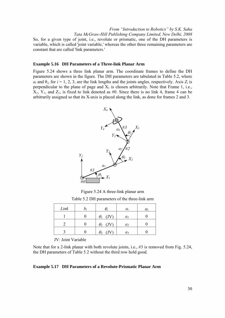
Example 5.16 DH Parameters of a Three-link Planar Arm
Figure 5.24 shows a three link planar arm. The coordinate frames to define the DH parameters are shown in the figure. The DH parameters are tabulated in Table 5.2, where ai and θi, for i = 1, 2, 3, are the link lengths and the joints angles, respectively. Axis Zi is perpendicular to the plane of page and X1 is chosen arbitrarily. Note that Frame 1, i.e., X1, Y1, and Z1, is fixed to link denoted as #0. Since there is no link 4, frame 4 can be arbitrarily assigned so that its X-axis is placed along the link, as done for frames 2 and 3.
Figure 5.24 A three-link planar arm
Table 5.2 DH parameters of the three-link arm
Link bi θi ai αi
1 0 θ1 (JV) a1 0
2 0 θ2 (JV) a2 0
3 0 θ3 (JV) a3 0
JV: Joint Variable
Note that for a 2-link planar with both revolute joints, i.e., #3 is removed from Fig. 5.24, the DH parameters of Table 5.2 without the third row hold good.
Example 5.17 DH Parameters of a Revolute-Prismatic Planar Arm
X1
X3
X2
X4
Y2 Y2
Y3 Y4
θ1
θ2
θ3 a3
a2
a1
#0
#1
#2
#3
From “Introduction to Robotics” by S.K. Saha Tata McGraw-Hill Publishing Company Limited, New Delhi, 2008
31
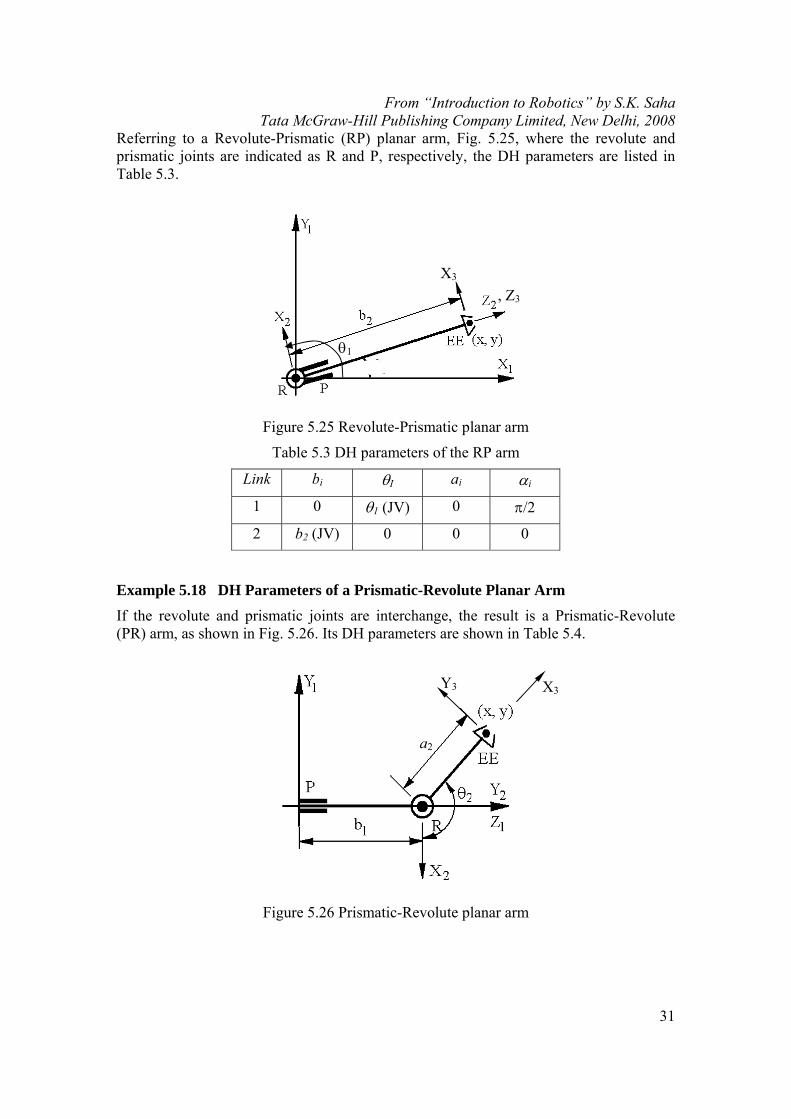
Referring to a Revolute-Prismatic (RP) planar arm, Fig. 5.25, where the revolute and prismatic joints are indicated as R and P, respectively, the DH parameters are listed in Table 5.3.
Figure 5.25 Revolute-Prismatic planar arm
Table 5.3 DH parameters of the RP arm
Link bi θI ai αi
1 0 θ1 (JV) 0 π/2
2 b2 (JV) 0 0 0
Example 5.18 DH Parameters of a Prismatic-Revolute Planar Arm
If the revolute and prismatic joints are interchange, the result is a Prismatic-Revolute (PR) arm, as shown in Fig. 5.26. Its DH parameters are shown in Table 5.4.
Figure 5.26 Prismatic-Revolute planar arm
, Z3
X3
θ1
X3 Y3
a2
From “Introduction to Robotics” by S.K. Saha Tata McGraw-Hill Publishing Company Limited, New Delhi, 2008
32
Table 5.4 DH parameters of the PR arm
Link bi θI ai αi
1 b2 (JV) -π/2 0 π/2
2 0 θ2 (JV) a2 0
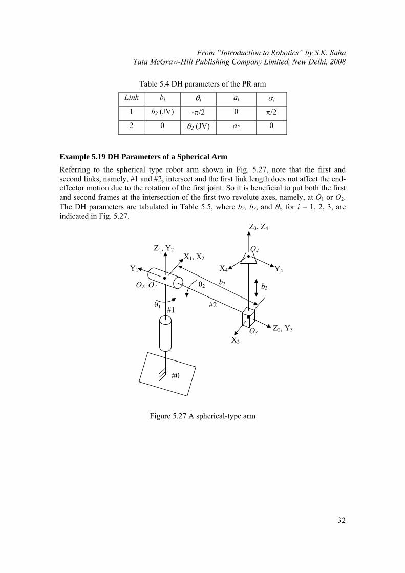
Example 5.19 DH Parameters of a Spherical Arm
Referring to the spherical type robot arm shown in Fig. 5.27, note that the first and second links, namely, #1 and #2, intersect and the first link length does not affect the end-effector motion due to the rotation of the first joint. So it is beneficial to put both the first and second frames at the intersection of the first two revolute axes, namely, at O1 or O2. The DH parameters are tabulated in Table 5.5, where b2, b3, and θi, for i = 1, 2, 3, are indicated in Fig. 5.27.
Figure 5.27 A spherical-type arm
#0
θ1 #1
Z1, Y2
Z2, Y3
#2
θ2
Y4 Y1 X1, X2
X3
O2, O2
X4
Z3, Z4
b3
O3
O4
b2
From “Introduction to Robotics” by S.K. Saha Tata McGraw-Hill Publishing Company Limited, New Delhi, 2008
33
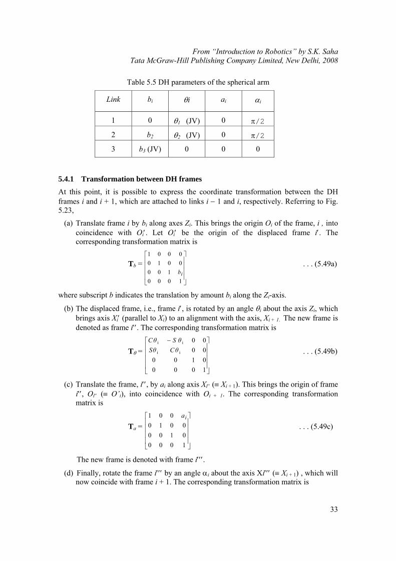
Table 5.5 DH parameters of the spherical arm
Link bi θi ai αi
1 0 θ1 (JV) 0 π/2
2 b2 θ2 (JV) 0 π/2
3 b3 (JV) 0 0 0
5.4.1 Transformation between DH frames
At this point, it is possible to express the coordinate transformation between the DH frames i and i + 1, which are attached to links i − 1 and i, respectively. Referring to Fig. 5.23,
(a) Translate frame i by bi along axes Zi. This brings the origin Oi of the frame, i , into coincidence with Oi′. Let Oi′ be the origin of the displaced frame i′. The corresponding transformation matrix is
Tb =
⎥⎥⎥⎥
⎦
⎤
⎢⎢⎢⎢
⎣
⎡
1000100
00100001
ib . . . (5.49a)
where subscript b indicates the translation by amount bi along the Zi-axis.
(b) The displaced frame, i.e., frame i′, is rotated by an angle θi about the axis Zi, which brings axis Xi′ (parallel to Xi) to an alignment with the axis, Xi + 1. The new frame is denoted as frame i′′. The corresponding transformation matrix is
Tθ =
⎥⎥⎥⎥
⎦
⎤
⎢⎢⎢⎢
⎣
⎡ −
100001000000
ii
ii
CθSθθSCθ
. . . (5.49b)
(c) Translate the frame, i′′, by ai along axis Xi′′ (≡ Xi + 1). This brings the origin of frame i′′, Oi′′ (≡ O’i), into coincidence with Oi + 1. The corresponding transformation matrix is
Ta =
⎥⎥⎥⎥
⎦
⎤
⎢⎢⎢⎢
⎣
⎡
100001000010
001 ia
. . . (5.49c)
The new frame is denoted with frame i′′′.
(d) Finally, rotate the frame i′′′ by an angle αi about the axis Xi′′′ (≡ Xi + 1) , which will now coincide with frame i + 1. The corresponding transformation matrix is
From “Introduction to Robotics” by S.K. Saha Tata McGraw-Hill Publishing Company Limited, New Delhi, 2008
34
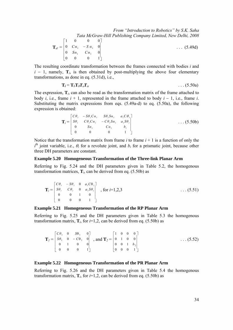
Tα′ =
⎥⎥⎥⎥
⎦
⎤
⎢⎢⎢⎢
⎣
⎡−
100000000001
ii
ii
CαSααSCα . . . (5.49d)
The resulting coordinate transformation between the frames connected with bodies i and i − 1, namely, Ti, is then obtained by post-multiplying the above four elementary transformations, as done in eq. (5.31d), i.e.,
Ti = TbTθTaTα . . . (5.50a)
The expression, Ti, can also be read as the transformation matrix of the frame attached to body i, i.e., frame i + 1, represented in the frame attached to body i − 1, i.e., frame i. Substituting the matrix expressions from eqs. (5.49a-d) to eq. (5.50a), the following expression is obtained:
Ti =
⎥⎥⎥⎥
⎦
⎤
⎢⎢⎢⎢
⎣
⎡−
−
10000 iii
iiiiiii
iiiiiii
bCαSαSθaSαCθCαCθSθCaSαSθCαSθCθ θ
. . . (5.50b)
Notice that the transformation matrix from frame i to frame i + 1 is a function of only the ith joint variable, i.e., θi for a revolute joint, and bi for a prismatic joint, because other three DH parameters are constant.
Example 5.20 Homogeneous Transformation of the Three-link Planar Arm
Referring to Fig. 5.24 and the DH parameters given in Table 5.2, the homogenous transformation matrices, Ti, can be derived from eq. (5.50b) as
Ti =
⎥⎥⎥⎥
⎦
⎤
⎢⎢⎢⎢
⎣
⎡ θ−
10000100
00
iiii
iiii
SθaCθSθCaSθCθ
, for i=1,2,3 . . . (5.51)
Example 5.21 Homogeneous Transformation of the RP Planar Arm
Referring to Fig. 5.25 and the DH parameters given in Table 5.3 the homogenous transformation matrix, Ti, for i=1,2, can be derived from eq. (5.50b) as
T1 =
⎥⎥⎥⎥
⎦
⎤
⎢⎢⎢⎢
⎣
⎡θ−θ
100000100000
11
11
CSθSCθ
, and T2 =
⎥⎥⎥⎥
⎦
⎤
⎢⎢⎢⎢
⎣
⎡
1000100
00100001
2b . . . (5.52)
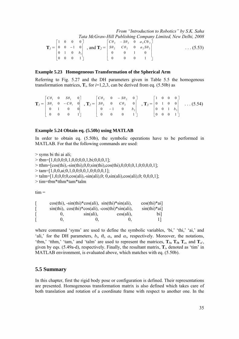
Example 5.22 Homogeneous Transformation of the PR Planar Arm
Referring to Fig. 5.26 and the DH parameters given in Table 5.4 the homogenous transformation matrix, Ti, for i=1,2, can be derived from eq. (5.50b) as
From “Introduction to Robotics” by S.K. Saha Tata McGraw-Hill Publishing Company Limited, New Delhi, 2008
35
T1 =
⎥⎥⎥⎥
⎦
⎤
⎢⎢⎢⎢
⎣
⎡−
1000010
01000001
1b, and T2 =
⎥⎥⎥⎥
⎦
⎤
⎢⎢⎢⎢
⎣
⎡ θ−
10000100
00
2222
2222
SθaCθSθCaSθCθ
. . . (5.53)
Example 5.23 Homogeneous Transformation of the Spherical Arm
Referring to Fig. 5.27 and the DH parameters given in Table 5.5 the homogenous transformation matrices, Ti, for i=1,2,3, can be derived from eq. (5.50b) as
T1 =
⎥⎥⎥⎥
⎦
⎤
⎢⎢⎢⎢
⎣
⎡−
100000100000
11
11
CθSθSθCθ
, T2 =
⎥⎥⎥⎥
⎦
⎤
⎢⎢⎢⎢
⎣
⎡
−
−
1000010
0000
2
22
22
bCθSθ
SθCθ
, T3 =
⎥⎥⎥⎥
⎦
⎤
⎢⎢⎢⎢
⎣
⎡
1000100
00100001
3b . . . (5.54)
Example 5.24 Obtain eq. (5.50b) using MATLAB
In order to obtain eq. (5.50b), the symbolic operations have to be performed in MATLAB. For that the following commands are used: > syms bi thi ai ali; > tbm=[1,0,0,0;0,1,0,0;0,0,1,bi;0,0,0,1]; > tthm=[cos(thi),-sin(thi),0,0;sin(thi),cos(thi),0,0;0,0,1,0;0,0,0,1]; > tam=[1,0,0,ai;0,1,0,0;0,0,1,0;0,0,0,1]; > talm=[1,0,0,0;0,cos(ali),-sin(ali),0; 0,sin(ali),cos(ali),0; 0,0,0,1]; > tim=tbm*tthm*tam*talm tim = [ cos(thi), -sin(thi)*cos(ali), sin(thi)*sin(ali), cos(thi)*ai] [ sin(thi), cos(thi)*cos(ali), -cos(thi)*sin(ali), sin(thi)*ai] [ 0, sin(ali), cos(ali), bi] [ 0, 0, 0, 1] where command ‘syms’ are used to define the symbolic variables, ‘bi,’ ‘thi,’ ‘ai,’ and ‘ali,’ for the DH parameters, bi, θi, ai, and αi, respectively. Moreover, the notations, ‘tbm,’ ‘tthm,’ ‘tam,’ and ‘talm’ are used to represent the matrices, Tb, Tθ, Ta, and Tα′, given by eqs. (5.49a-d), respectively. Finally, the resultant matrix, Ti, denoted as ‘tim’ in MATLAB environment, is evaluated above, which matches with eq. (5.50b). 5.5 Summary In this chapter, first the rigid body pose or configuration is defined. Their representations are presented. Homogeneous transformation matrix is also defined which takes care of both translation and rotation of a coordinate frame with respect to another one. In the
From “Introduction to Robotics” by S.K. Saha Tata McGraw-Hill Publishing Company Limited, New Delhi, 2008
36
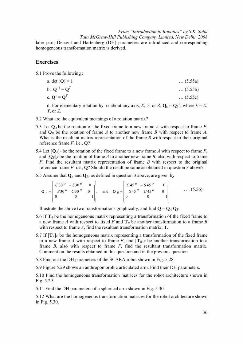
later part, Denavit and Hartenberg (DH) parameters are introduced and corresponding homogeneous transformation matrix is derived.
Exercises 5.1 Prove the following :
a. det (Q) = 1 … (5.55a)
b. Q−1 = QT … (5.55b)
c. Q’ = QT … (5.55c)
d. For elementary rotation by α about any axis, X, Y, or Z, Qk = QkT, where k = X,
Y, or Z.
5.2 What are the equivalent meanings of a rotation matrix?
5.3 Let QA be the rotation of the fixed frame to a new frame A with respect to frame F, and QB be the rotation of frame A to another new frame B with respect to frame A. What is the resultant matrix representation of the frame B with respect to their original reference frame F, i.e., Q?
5.4 Let [QA]F be the rotation of the fixed frame to a new frame A with respect to frame F, and [QB]F be the rotation of frame A to another new frame B, also with respect to frame F. Find the resultant matrix representation of frame B with respect to the original reference frame F, i.e., Q? Should the result be same as obtained in question 3 above?
5.5 Assume that QA and QB, as defined in question 3 above, are given by
⎥⎥⎥⎥
⎦
⎤
⎢⎢⎢⎢
⎣
⎡ −
=
⎥⎥⎥⎥
⎦
⎤
⎢⎢⎢⎢
⎣
⎡ −
=
04545
10004545and,
03030
10003030
oSoCoCoS
oSoCoCoS BA QQ . . . (5.56)
Illustrate the above two transformations graphically, and find Q = QA QB.
5.6 If TA be the homogeneous matrix representing a transformation of the fixed frame to a new frame A with respect to fixed F and TB be another transformation to a frame B with respect to frame A, find the resultant transformation matrix, T.
5.7 If [TA]F be the homogeneous matrix representing a transformation of the fixed frame to a new frame A with respect to frame F, and [TB]F be another transformation to a frame B, also with respect to frame F, find the resultant transformation matrix. Comment on the results obtained in this question and in the previous question.
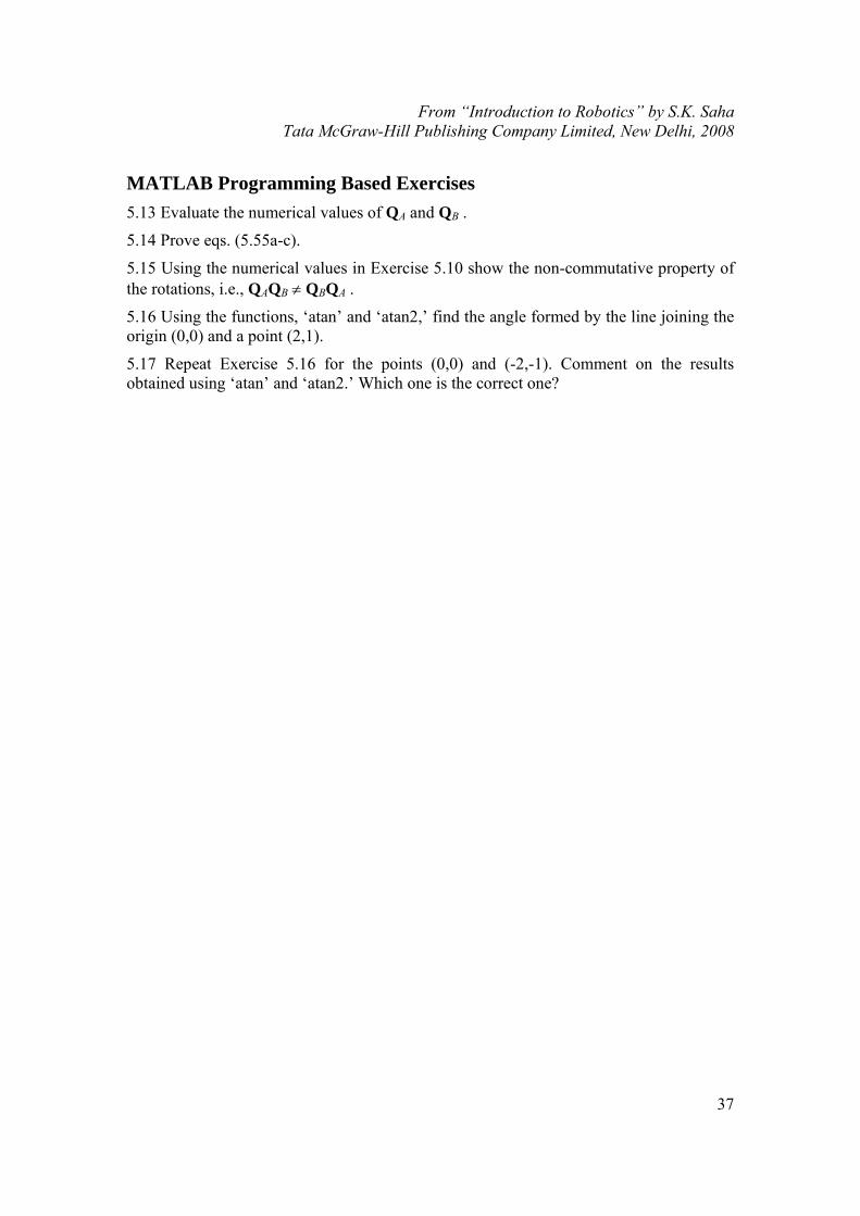
5.8 Find out the DH parameters of the SCARA robot shown in Fig. 5.28.
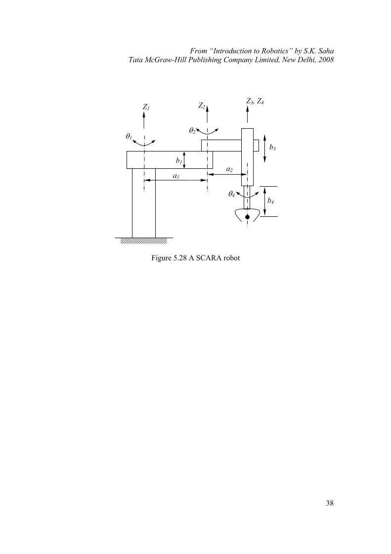
5.9 Figure 5.29 shows an anthropomorphic articulated arm. Find their DH parameters.
5.10 Find the homogeneous transformation matrices for the robot architecture shown in Fig. 5.29.
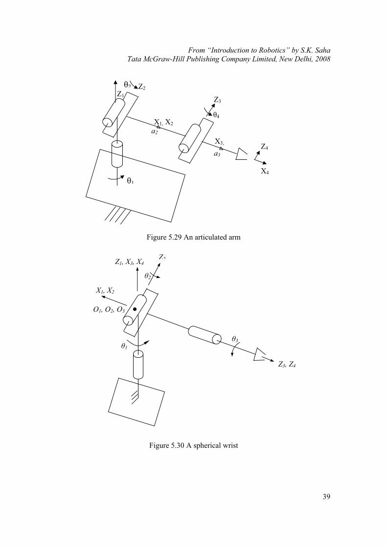
5.11 Find the DH parameters of a spherical arm shown in Fig. 5.30.
5.12 What are the homogeneous transformation matrices for the robot architecture shown in Fig. 5.30.
From “Introduction to Robotics” by S.K. Saha Tata McGraw-Hill Publishing Company Limited, New Delhi, 2008
37
MATLAB Programming Based Exercises 5.13 Evaluate the numerical values of QA and QB .
5.14 Prove eqs. (5.55a-c).
5.15 Using the numerical values in Exercise 5.10 show the non-commutative property of the rotations, i.e., QAQB ≠ QBQA .
5.16 Using the functions, ‘atan’ and ‘atan2,’ find the angle formed by the line joining the origin (0,0) and a point (2,1).
5.17 Repeat Exercise 5.16 for the points (0,0) and (-2,-1). Comment on the results obtained using ‘atan’ and ‘atan2.’ Which one is the correct one?
From “Introduction to Robotics” by S.K. Saha Tata McGraw-Hill Publishing Company Limited, New Delhi, 2008
38
Figure 5.28 A SCARA robot
Z1 Z3, Z4
θ1 θ2
b3
θ4
Z2
a2 a1
b1
b4
From “Introduction to Robotics” by S.K. Saha Tata McGraw-Hill Publishing Company Limited, New Delhi, 2008
39
Figure 5.29 An articulated arm
Figure 5.30 A spherical wrist
X1, X2
Z1, X3, X4 Z2
θ3
θ2
Z3, Z4
O1, O2, O3
θ1
X1, X2
Z1
Z2 θ2
θ1
a2
a3
X3, Z4
Z3
θ4
X4