stabilization and navigation for an autonomous underwater ... · iii declaration of authorship i,...

ENSTA BRETAGNE

MASTER THESIS

Stabilization and Navigation for anAutonomous Underwater Vehicle

Author:Nima MEHDI

School Supervisor:Dr. Benoit ZERR

Supervisor:Pierre Budan

A master thesis submitted in fulfillment of the requirementsfor the title of Engineer

with the participation of

Notilo+

August 23, 2017

http://www.ensta-bretagne.fr/

https://ibubble.camera/

iii

Declaration of AuthorshipI, Nima MEHDI, declare that this thesis titled, “Stabilization and Navigation foran Autonomous Underwater Vehicle” and the work presented in it are my own. Iconfirm that:

• This work was done wholly or mainly while in candidature for a research de-gree at this University.

• Where any part of this thesis has previously been submitted for a degree orany other qualification at this University or any other institution, this has beenclearly stated.

• Where I have consulted the published work of others, this is always clearlyattributed.

• Where I have quoted from the work of others, the source is always given. Withthe exception of such quotations, this thesis is entirely my own work.

• I have acknowledged all main sources of help.

• Where the thesis is based on work done by myself jointly with others, I havemade clear exactly what was done by others and what I have contributed my-self.

Signed:Mehdi Nima

v

“First Law: A robot may not injure a human being, or, through inaction, allow a humanbeing to come to harm.Second Law: A robot must obey the orders given it by human beings except where suchorders would conflict with the first law.Third Law : A robot must protect its own existence as long as such protection does notconflict with the First or Second Law. ”

Isaac Asimov

vii

ENSTA Bretagne

AbstractENSTA Bretagne

Robotics

Master of Science in Engineering

Stabilization and Navigation for an Autonomous Underwater Vehicle

by Nima MEHDI

This report investigates the problem of stabilization and smooth motion of autonomousunderwater vehicles through control and navigation methods. A hydrodynamicmodel of the robot is suggested and through simulation and identifications, we de-termine the characteristics of the system in question. Then a classic PID controller isused to test the control. To improve stability, an Extented Kalman Filter is also ad-dressed. Eventually, navigation strategies are presented to study the robot motion.

Ce rapport aborde la problématique de stabilisation d’un robot sous marin dansle cadre d’une poursuite de cible. Dans un premier temps, nous proposons unmodèle physique du drone afin de réaliser des simulations et à l’aide de méth-odes d’identifications, de déduire de manière plus précise les caractéristiques dusystème. Les résultats nous permettent de mener une étude sur le contrôle du sys-tème à travers de simples PID en série. Finalement, des stratégies de navigation sontproposées afin de déterminer le comportement général du drone.



http://department.university.com

ix

AcknowledgementsI would like to give my thanks to the Notilo+ team for the warm welcome and

their support for this work.

I would like to thank Pierre Budan, for supervising me with patience and peda-gogy. I would like to thank Sam Tabia from Sogilis for introducing me to the projectand offering me an external point of view regarding my missions.

I would like to thank professors Jean-Marc Laurens, Fabrice LeBars and BenoitZerr for answering my questions and guiding me during the internship.

I would like to thank especially my family for their support for theses years spentat ENSTA Bretagne and were an incredible help for all this time being.

xi

Contents

Declaration of Authorship iii

Abstract vii

Acknowledgements ix

1 Preface 11.1 Introduction . . . . . . . . . . . . . . . . . . . . . . . . . . . . . . . . . . 11.2 About the craft . . . . . . . . . . . . . . . . . . . . . . . . . . . . . . . . . 11.3 Objectives . . . . . . . . . . . . . . . . . . . . . . . . . . . . . . . . . . . 2

2 AUV Modeling 32.1 Architecture . . . . . . . . . . . . . . . . . . . . . . . . . . . . . . . . . . 3

2.1.1 Reference Frames . . . . . . . . . . . . . . . . . . . . . . . . . . . 3Earth Fixed Frame . . . . . . . . . . . . . . . . . . . . . . . . . . 3Target Frame . . . . . . . . . . . . . . . . . . . . . . . . . . . . . 3BODY Frame . . . . . . . . . . . . . . . . . . . . . . . . . . . . . 3

2.1.2 Hypothesis regarding the AUV . . . . . . . . . . . . . . . . . . . 52.2 Equations of motion . . . . . . . . . . . . . . . . . . . . . . . . . . . . . 5

2.2.1 Kinematics . . . . . . . . . . . . . . . . . . . . . . . . . . . . . . . 5Euler Angles Transformation . . . . . . . . . . . . . . . . . . . . 6Quaternions representation . . . . . . . . . . . . . . . . . . . . . 6

2.2.2 Rigid-Body Kinetics . . . . . . . . . . . . . . . . . . . . . . . . . 7Rigid Body Inertial Matrix . . . . . . . . . . . . . . . . . . . . . . 7Coriolis-Centripetal Matrix . . . . . . . . . . . . . . . . . . . . . 7Thrusters Forces . . . . . . . . . . . . . . . . . . . . . . . . . . . 8

2.2.3 Hydrostatics . . . . . . . . . . . . . . . . . . . . . . . . . . . . . . 92.2.4 Hydrodynamics Forces . . . . . . . . . . . . . . . . . . . . . . . 9

Added Mass and Added Centripetal Matrices . . . . . . . . . . 10Damping forces . . . . . . . . . . . . . . . . . . . . . . . . . . . . 11

2.2.5 Waves and Wind influences . . . . . . . . . . . . . . . . . . . . . 122.2.6 Motor Modeling . . . . . . . . . . . . . . . . . . . . . . . . . . . 13

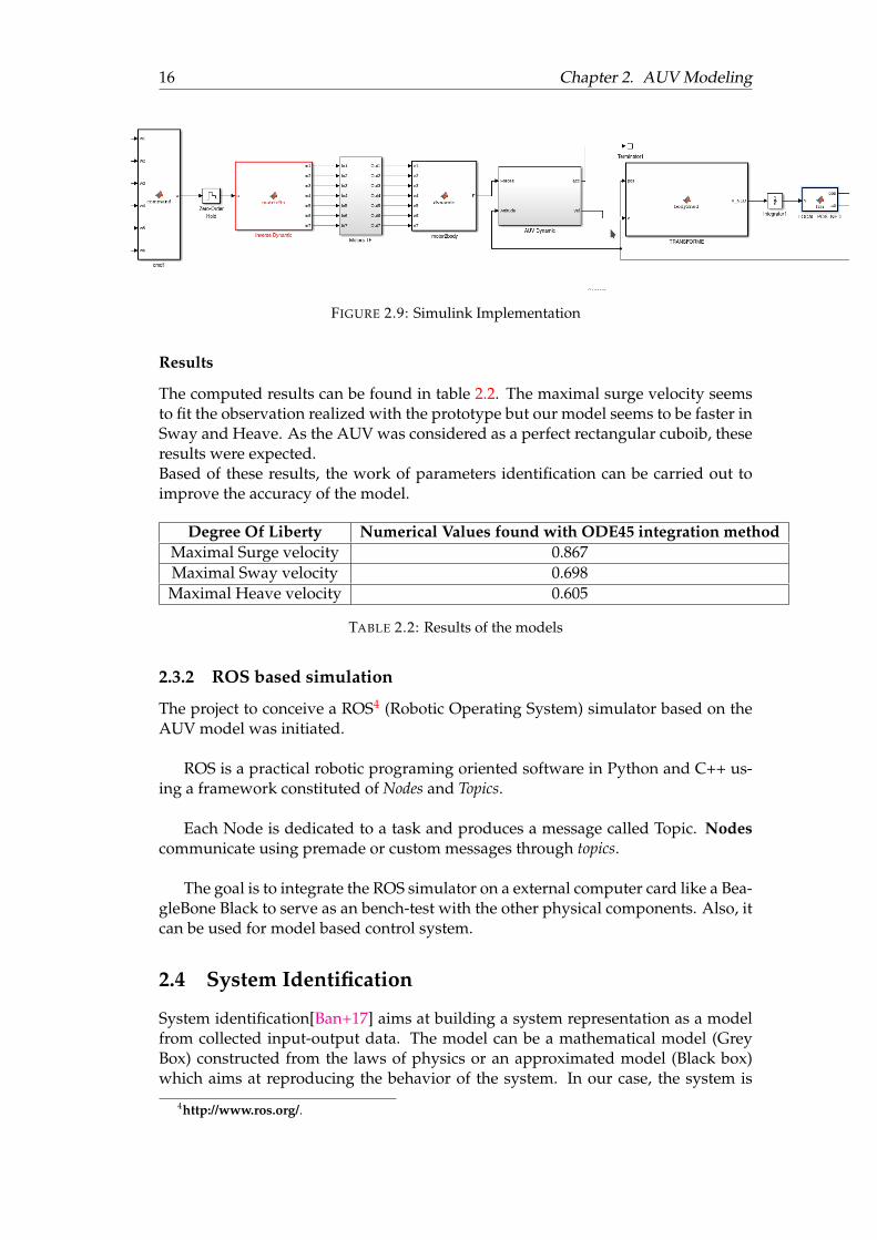
2.3 Computer Model . . . . . . . . . . . . . . . . . . . . . . . . . . . . . . . 152.3.1 Simulink Model . . . . . . . . . . . . . . . . . . . . . . . . . . . . 15

Results . . . . . . . . . . . . . . . . . . . . . . . . . . . . . . . . . 162.3.2 ROS based simulation . . . . . . . . . . . . . . . . . . . . . . . . 16

2.4 System Identification . . . . . . . . . . . . . . . . . . . . . . . . . . . . . 162.4.1 Procedure . . . . . . . . . . . . . . . . . . . . . . . . . . . . . . . 172.4.2 Grey Model Identification . . . . . . . . . . . . . . . . . . . . . . 172.4.3 State space identification . . . . . . . . . . . . . . . . . . . . . . . 182.4.4 Transfer function identification . . . . . . . . . . . . . . . . . . . 19

xii

3 Stabilization and Motion Regulation 233.1 Current State of the Control System . . . . . . . . . . . . . . . . . . . . 23

3.1.1 Attitude Control . . . . . . . . . . . . . . . . . . . . . . . . . . . 233.1.2 Position control . . . . . . . . . . . . . . . . . . . . . . . . . . . . 24

North and East Control . . . . . . . . . . . . . . . . . . . . . . . 24Depth Control . . . . . . . . . . . . . . . . . . . . . . . . . . . . . 24

3.2 Controller design . . . . . . . . . . . . . . . . . . . . . . . . . . . . . . . 243.3 PID Algorithm . . . . . . . . . . . . . . . . . . . . . . . . . . . . . . . . . 273.4 Hysteresis Thresholding . . . . . . . . . . . . . . . . . . . . . . . . . . . 283.5 Extended Kalman Filter . . . . . . . . . . . . . . . . . . . . . . . . . . . 28

3.5.1 Native Inertial Navigation Filter . . . . . . . . . . . . . . . . . . 283.5.2 Extended Kalman Filter . . . . . . . . . . . . . . . . . . . . . . . 29

4 Guidance and Motion Control 314.1 2D Tracking . . . . . . . . . . . . . . . . . . . . . . . . . . . . . . . . . . 31

Pursuit . . . . . . . . . . . . . . . . . . . . . . . . . . . . . . . . . 32Bezier Polynomial . . . . . . . . . . . . . . . . . . . . . . . . . . 33Yaw and Depth Guidance . . . . . . . . . . . . . . . . . . . . . . 33

4.1.1 3D Tracking . . . . . . . . . . . . . . . . . . . . . . . . . . . . . . 34Results . . . . . . . . . . . . . . . . . . . . . . . . . . . . . . . . . 34

5 Conclusion 37

Bibliography 41

xiii

List of Figures

1.1 Technical presentation of the iBubble prototype "Beluga" . . . . . . . . . 11.2 The iBubble prototype, Beluga, during a test session . . . . . . . . . . . 2

2.1 The BODY frame illustrated with respect to the NED frame . . . . . . . 42.2 Schematic representation of the AUV . . . . . . . . . . . . . . . . . . . . 82.3 The Weight and Buoyancy forces on an underwater vehicle . . . . . . . 92.4 Two-dimensional coefficient for a rectangular cross section . . . . . . . 102.5 The T200 Thruster which is a waterproof brushless motor . . . . . . . . 132.6 Thrust response in function of the Pulse Width Modulation send to

the ESC . . . . . . . . . . . . . . . . . . . . . . . . . . . . . . . . . . . . . 132.7 Measured Input And Output from the motor for a PWM of 1600 . . . . 142.8 The simulated output has a 80% match with the measurement . . . . . 152.9 Simulink Implementation . . . . . . . . . . . . . . . . . . . . . . . . . . 162.10 Predicted outputs and simulated outputs . . . . . . . . . . . . . . . . . 192.11 Step response on the third thrust . . . . . . . . . . . . . . . . . . . . . . 202.12 Step response on the third thrust . . . . . . . . . . . . . . . . . . . . . . 202.13 dot line : simulated step response, solid line : measured step response 21

3.1 Attitude Control . . . . . . . . . . . . . . . . . . . . . . . . . . . . . . . . 233.2 Current Control System . . . . . . . . . . . . . . . . . . . . . . . . . . . 243.3 . . . . . . . . . . . . . . . . . . . . . . . . . . . . . . . . . . . . . . . . . 243.4 Controllers for the Position and the Velocity . . . . . . . . . . . . . . . . 253.5 Controlling the position . . . . . . . . . . . . . . . . . . . . . . . . . . . 253.6 Controlling the velocity . . . . . . . . . . . . . . . . . . . . . . . . . . . 263.7 Controlling both the position and the velocity . . . . . . . . . . . . . . . 263.8 Controller with anti-windup . . . . . . . . . . . . . . . . . . . . . . . . . 273.9 Estimation of the North Position of the AUV . . . . . . . . . . . . . . . 29

4.1 2D trajectory planing: the cross represents the diver and the circle thesetpoint assumed as target . . . . . . . . . . . . . . . . . . . . . . . . . . 31

4.2 Follow-me scenario . . . . . . . . . . . . . . . . . . . . . . . . . . . . . . 324.3 Come to me scenario . . . . . . . . . . . . . . . . . . . . . . . . . . . . . 334.4 Illustration of second-order B-splines . . . . . . . . . . . . . . . . . . . . 334.5 . . . . . . . . . . . . . . . . . . . . . . . . . . . . . . . . . . . . . . . . . 344.6 . . . . . . . . . . . . . . . . . . . . . . . . . . . . . . . . . . . . . . . . . 354.7 Showing in blue, the desired pitch, in red the AUV pitch . . . . . . . . 35

1 The corroded motor . . . . . . . . . . . . . . . . . . . . . . . . . . . . . . 40

xv

List of Tables

2.1 AUV Characteristics . . . . . . . . . . . . . . . . . . . . . . . . . . . . . 52.2 Results of the models . . . . . . . . . . . . . . . . . . . . . . . . . . . . . 16

xvii

List of Abbreviations

AUV Autonomous Underwater VehicleNED North East DownDOF Degree Of FreedomIMU Inertial Measurement UnitPID Proportional Integral Derivative

1

Chapter 1

Preface

1.1 Introduction

Remotely operated vehicles and by extension autonomous vehicles play significantsroles in the public sector and within the industrial sector as well. They are used fordifferent field of expertises such as surveillance and exploration. Drones as they areusually called, have started to enter the private sphere as high-tech devices to en-hance the experience in their recreational activities.

Notilo+ is a newborn company which already gathered a high amount of fundsfor the project iBubble. With iBubble, Notilo+ seeks to offer an autonomous underwa-ter vehicle(AUV) able to assist divers as a remote and automated camera. The smallsubmarine has to be able to pinpoint the diver position and follow him.

The development of iBubble had led to two expected models. A first modelwith limited computing power is intended for a larger audience. The second modelwould be intended for industrial and military use, with enhanced capacities relativeto the former. Using computer vision and acoustic localization, it will be able toachieve missions such as hull inspection, determination of a fish population andeven assisting combat divers.

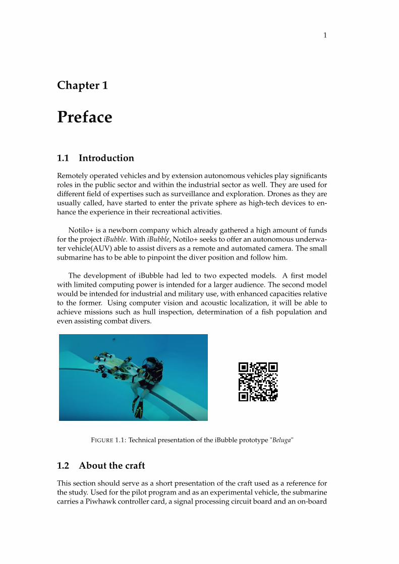
FIGURE 1.1: Technical presentation of the iBubble prototype "Beluga"

1.2 About the craft

This section should serve as a short presentation of the craft used as a reference forthe study. Used for the pilot program and as an experimental vehicle, the submarinecarries a Piwhawk controller card, a signal processing circuit board and an on-board

2 Chapter 1. Preface

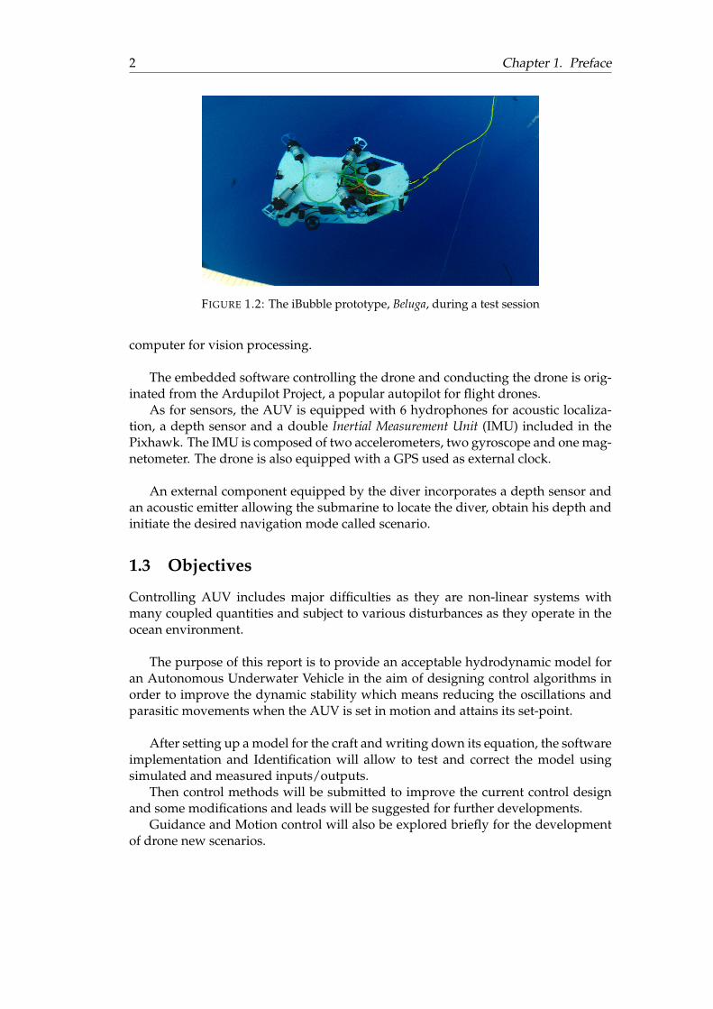
FIGURE 1.2: The iBubble prototype, Beluga, during a test session

computer for vision processing.

The embedded software controlling the drone and conducting the drone is orig-inated from the Ardupilot Project, a popular autopilot for flight drones.

As for sensors, the AUV is equipped with 6 hydrophones for acoustic localiza-tion, a depth sensor and a double Inertial Measurement Unit (IMU) included in thePixhawk. The IMU is composed of two accelerometers, two gyroscope and one mag-netometer. The drone is also equipped with a GPS used as external clock.

An external component equipped by the diver incorporates a depth sensor andan acoustic emitter allowing the submarine to locate the diver, obtain his depth andinitiate the desired navigation mode called scenario.

1.3 Objectives

Controlling AUV includes major difficulties as they are non-linear systems withmany coupled quantities and subject to various disturbances as they operate in theocean environment.

The purpose of this report is to provide an acceptable hydrodynamic model foran Autonomous Underwater Vehicle in the aim of designing control algorithms inorder to improve the dynamic stability which means reducing the oscillations andparasitic movements when the AUV is set in motion and attains its set-point.

After setting up a model for the craft and writing down its equation, the softwareimplementation and Identification will allow to test and correct the model usingsimulated and measured inputs/outputs.

Then control methods will be submitted to improve the current control designand some modifications and leads will be suggested for further developments.

Guidance and Motion control will also be explored briefly for the developmentof drone new scenarios.

3

Chapter 2

AUV Modeling

The motivation to obtain a model surges to the need of a better understanding of thesystem. Empirical and computing methods cannot be used as they were not avail-able, establishing a model using geometric and physicals considerations became amust.

Once the model is established, simulations using actual inputs, recorded duringtest sessions, allow to confirm and tune the model.

2.1 Architecture

2.1.1 Reference Frames

For marine crafts moving with six degrees of freedom[FOS11], six independents co-ordinates are necessary to determine the position and orientation.

Earth Fixed Frame

The geographic reference frame used is the North East Down, noted here as {n} co-ordinate system whose origin is defined relative to the Earth reference frame. Forthis system, the origin On is fixed such as the entry point of the robot underwater.

• The xn axis will be pointing to the North.

• The yn axis points to the East.

• The zn axis is pointing downward making the NED frame is a right handedframe.

Target Frame

The second frame of reference will be fixed to the diver as origin. The axis orienta-tions are the same as the NED coordinates. This frame {t} will be the projection ofthe NED Frame on the plane of depth zt.

BODY Frame

The body-fixed reference frame with origin ob is associated with the vehicle wherethe body axis are chosen to coincide with the axes of inertia. It is also a right handedcoordinate system. It will be noted as {b}.

• The xb axis will be pointing forward.

4 Chapter 2. AUV Modeling

FIGURE 2.1: The BODY frame illustrated with respect to the NEDframe

• The yb axis points right of the previous axis.

• The zb axis is going from top to bottom.

Some body-fixed reference points will be expressed within {b}:

• CO geometric center of the vehicle

• CG center of gravity

• CB center of buoyancy

For marine craft the following notation will be adopted for vectors in the coordi-nate systems {b} and {e}

pnb/n = position of ob with respect to n expressed in {n}

vbb/n = linear velocity of ob with respect to n expressed in {b}

ωbb/n = angular velocity of ob with respect to n expressed in {b}

fnb = external forces with the line of action trough the point ob expressed in {n}

mnb = moments about the point ob expressed in {n}

Using SNAME(1950) notations for marine vessels, the useful quantities can beexpressed in the vectorial setting, in regard of the different frames defined earlier.

2.2. Equations of motion 5

NED Position pnb/n =

NED

Attitude (Euler Angles) Θnb =

φθψ

Body Fixed Velocity vbb/n =

uvw

Body fixed angular Velocity ωbb/n =

pqr

Body fixed forces f bb =

XYZ

Body fixed moments mbb =

KMN

2.1.2 Hypothesis regarding the AUV

The prototype was assimilated to a rectangular cuboid. As we lack of numericaltools to determinate the values of empirical mechanical coefficients, We consideredsome simplification while trying to stay the most trustful to the actual prototype.

The rectangular cuboid was assigned with a mass m, homogeneously distributedto the rigid body. With a length l, a width b and a height h. The density is d.

The A.U.V is equipped with 7 propellers allowing to move according to the 6 de-grees of freedom. The motors are split according to each degree: 4 for the surge,swayand yaw as 3 are meant to actuate the roll, pitch and heave.

Therefore the AUV does not have a ballast: the vector ~GB is constant. The modelis defined in the following table.

Size 0.800m (l) 0.600m (b) 0.400m (h)Weight 24 kgVolume 26 L

Degree of Freedom 6 DOFPropulsion 4 horizontal and 3 vertical propellers

Speed 1.6 knots (Surge) and 0.58 knots (Sway)Depth Rating 60m

TABLE 2.1: AUV Characteristics

2.2 Equations of motion

The marine craft equations of motions can be written in a vectorial setting accordingto Fossen[FOS11]:

η = JΘν (2.1)Mν + C(ν)ν + D(ν)ν + g(η) + g0 = τ + τwind + τwave (2.2)

2.2.1 Kinematics

As the AUV possesses six degree of freedom, using the notations defined in 2.1.1,the general motion of the submarine is expressed by the following vectors:


η =

[pnb/nΘnb

], ν =

[vbb/nωbb/n

], τ =

[f bbmbb

]The AUV position will be expressed with {n} where the origin would be super-

posed to the {t} origin at the water surface.

Euler Angles Transformation

Referring to Fossen [FOS11], the six DOF kinematics (2.1) equations can be expressedas: [

pnb/nΘnb

]=

[Rnb (Θnb) 03×3

03×3 TΘ(Θnb)

][vbb/nωbb/n

](2.3)

Rnb is the rotational matrix between the NED frame and the body-fixed frame,

expressed with the Euler angles.

Rnb =

cψcθ −sψcφ+ cψsθsφ sψsφ+ cψcφsθsψcθ cψcφ+ sφsθsψ −cψsφ+ sθsψcφ−sθ cθsφ cθcφ

(2.4)

where s· = sin(·) and c· = cos(·)The body fixed angular velocity ωbb/n can’t be integrated to obtain actual coordi-

nates as it does not hold any physical significance. But Θnb does. TΘ is the transfor-mation matrix between the angular velocities of the body to NED frame.

Tθ(Θnb) =

1 sφtθ cφtθ0 cφ −sφ0 sφ

cθcφcθ

(2.5)

where t· = tan(·).Notice that TΘ(Θnb) is undefined for θ = 90 deg. As vehicles with 6 DOF physicallyallow this value for θ, the singularity leads to computational errors called gimbal lock.To avoid any potential singularity, the quaternion representation will be favored incomputational implementations.

Quaternions representation

An alternative to Euler Angles representation is the unit quaternion representation.

q = [η, ε1, ε2, ε3]T (2.6)

A unit quaternion is defined as an element of the set Q:

Q = {q|qqT = 1, q = [η, ε], ε ∈ R3 and η ∈ R} (2.7)

Then Rnb and Tθ(Θnb) can be rewritten as

Rnb =

1− 2(ε22 + ε23) 2(ε1ε2 − ε3η) 2(ε1ε3 + ε2η)2(ε1ε2 + ε3η) 1− 2(ε21 + ε23) 2(ε2ε3 − ε1η)2(ε1ε3 − ε2η) 2(ε2ε3 − ε1η) 1− 2(ε21 + ε22)

(2.8)

and


Tq(q) =1

2

−ε1 s− ε2 −ε3η −ε3 sε2ε3 η −ε1−ε2 ε1 η

(2.9)

2.2.2 Rigid-Body Kinetics

According to Fossen[FOS11] the rigid body kinetics are:

Mrbν + Crb(ν)ν = τrb (2.10)

Each quantities can be calculated by writing down the Euler’s first and secondaxioms expressing the conservation of linear and angular momentums. The detailscan be found in [FOS11] and [BOE10].

Rigid Body Inertial Matrix

Defining the vector from O (geometric center of the rigid body ) to G (center of grav-ity of the rigid body) as rbg = [xg, yg, zg]

T and the cross-product matrix S defined as

S(rbg) =

0 −zg ygzg 0 −xg−yg xg 0

The representation of the inertial mass matrix is

Mrb =

[mI3×3 −mS(rbg)

mS(rbg) Ib

](2.11)

where I3×3 is an identity matrix and Ib is the inertial matrix. The hypotheses in-troduced earlier allow to consider the body axes to coincide with the axes of inertiaand the presence of symmetry on the three planes.

Hence, for a cuboid the inertial matrix can be written as:

Ib =

m12(b2 + h2) 0 00 m

12(l2 + h2) 00 0 m

12(b2 + l2)

(2.12)

By considering the origin O coincides with G allows to obtain a simplified inertialmatrix with only diagonal terms:

Mrb =

m 0 0 0 0 00 m 0 0 0 00 0 m 0 0 00 0 0 m

12(b2 + h2) 0 00 0 0 0 m

12(l2 + h2) 00 0 0 0 0 m

12(b2 + b2)

(2.13)

Coriolis-Centripetal Matrix

The determination of the Coriolis and centripetal matrix is given in [FOS11] and[FOS94] with greater details. The Lagrangian parametrization was chosen for its


simplicity:

Crb =

[03×3 −mS(v1)−mS(v2)S(rbg)

−mS(v1)−mS(v2)S(rbg) −S(Ibv2)

](2.14)

Thrusters Forces

FIGURE 2.2: Schematic representation of the AUV

The motor i delivers a thrust of Ti and the forces applied to the rigid body can bewritten as τrb = [X,Y, Z,K,M,N ]T . Taking in account the position of each thruster,the forces and moments can be expressed as:

X = (T1 + T2 + T3 + T4) cosα

Y = (T2 + T4 − T1 − T3) sinα

Z = T5 + T6 + T7

K = lbT5 − lbT6

M = −laT5 − laT6 + lcT7

N = (lx sinα+ ly cosα)(T2 + T3 − T1 − T4)

(2.15)

with α = 30 deg, la = 150mm, lb = 259mm, lc = 300mm, lx = 450mm, ly =350mm

It can be rewritten in the matricial setting as:


XYZKMN

=

cosα cosα cosα cosα 0 0 0− sinα sinα − sinα sinα 0 0 0

0 0 0 0 1 1 10 0 0 0 lb −lb 00 0 0 0 −la −la lc−C C C −C 0 0 0

T1

T2

T3

T4

T5

T6

T7

(2.16)

with C = lx sinα+ ly cosα.

2.2.3 Hydrostatics

For a submerged vehicle of mass m, ∇ the volume of displaced fluid by the vehicle,g the acceleration of gravity (positive downwards) and ρ the water density. Thesubmerged weight of the body and buoyancy force are written as

W = mg, B = ρg∇ (2.17)

FIGURE 2.3: The Weight and Buoyancy forces on an underwater ve-hicle

Let CB = [xb, yb, zb]T and CG = [xg, yg, zg]

T , the vector g(η) becomes:

g(η) =

(W −B) sin θ−(W −B) cos θ sinφ−(W −B) cos θ cosφ

−(ygW − ybB) cos θ cosφ+ (zgW − zbB) cos θ sinφ(zgW − zbB) sin θ + (xgW − xbB) cos θ cosφ−(xgW − xbB) cos θ sinφ− (ygW − ybB) sin θ

(2.18)

As the AUV does not have any ballast or self-balancing system, g0 does not exist.

2.2.4 Hydrodynamics Forces

For vehicles operating at water level depths below the wave-affected zone, the hy-drodynamic coefficients are independent of the wave excitation frequency. Thismean the added mass matrices can be considered as constant. In addition therewill be no potential damping.


The only hydrodynamic coefficients considered in this models are the systemadded inertia matrices MA and CA(νr) and D(νr) the damping matrix.

Added Mass and Added Centripetal Matrices

The coefficients of the added mass matrix will be calculated by using string theoryof slender bodies [FOS94].

The principle of strip theory involves dividing the submerged ship into a numberof strips. The two dimensional hydrodynamics coefficients for added mass can becomputed for each strip and are added following the length of the ship to yield thethree dimensional coefficients

For a submerged slender vehicle, the following formulas can be used:1

A11 = −Xu =

∫ L/2

−L/2A

(2D)11 (y, z)dx ≈ m (2.19)

A22 = −Yv =

∫ L/2

−L/2A

(2D)22 (y, z)dx (2.20)

A33 = −Zw =

∫ L/2

−L/2A

(2D)33 (y, z)dx (2.21)

A44 = −Kp =

∫ L/2

−L/2A

(2D)44 (y, z)dx (2.22)

A55 = −Mq =

∫ L/2

−L/2A

(2D)55 (y, z)dx (2.23)

A66 = −Nr =

∫ L/2

−L/2A

(2D)66 (y, z)dx (2.24)

(2.25)

Available tables[FOS94] give approximated added mass coefficients A(2D)ii :

FIGURE 2.4: Two-dimensional coefficient for a rectangular cross sec-tion

1The coefficient in surge can be approximated as the mass[YAN+15] for a cuboid and 0.1m for atorbedo shaped AUV


A22 = A33 = 1.5πρa2 with a =h

2(2.26)

The added mass coefficients for pitch, roll and yaw can be written according to[FOS94] as:

∫ L/2

−L/2A

(2D)44 (y, z)dx =

∫ B/2

−B/2y2A

(2D)33 (x, z)dy +

∫ H/2

−H/2z2A

(2D)22 (x, y)dz (2.27)∫ L/2

−L/2A

(2D)55 (y, z)dx =

∫ L/2

−L/2x2A

(2D)33 (y, z)dx+

∫ H/2

−H/2z2A

(2D)11 (x, z)dz (2.28)∫ L/2

−L/2A

(2D)66 (y, z)dx =

∫ B/2

−B/2y2A

(2D)11 (x, z)dy +

∫ L/2

−L/2x2A

(2D)22 (y, z)dx (2.29)

Which results2 to:

Xu = −mYv = −0.375πρh2l

Zw = −0.375πρh2l

Kp = −0.375πρh2

3(b3 + h3) (2.30)

Mq = −(0.375πρh2l3 +m

3lh3)

Nr = −(mb3

3l+ 0.375πρh2l3)

Hence, the added mass matrices for an underwater vehicle with 3 planes of sym-metry and moving in 6DOF can be written as follows:

MA = −diag([Xu, Yv, Zw,Kp,Mq, Nr]) (2.31)

CA(ν) =

0 0 0 0 −Zww Yvv0 0 0 Zww 0 −Xuu0 0 0 −Yvv Xuu 00 −Zww Yvv 0 −Nrr Mqq

Zww 0 Xuu Nrr 0 −Kpp−Yvv Xuu 0 −Mqq KpP 0

(2.32)

Damping forces

The wave-inducing damping does not contribute in the model. However, the hydro-dynamic damping taken into account will be:

Skin Friction:The linear term will be not considered in order to simplify the model. However

non linear skin friction will be approximated with the following formula:

2These values are heavily simplified and are used as a default choice


fs(u) = −1

2ρS(1 + k)CF (Rn)|u|u (2.33)

where ρ is the water density, S is the immersed surface of the vehicle. k is theform factor giving a viscous correction. Typically k = 0.25.

Cf can be calculated for turbulent flow with the ITTC’573 formula using theReynold number Rn. For a plane surface, the Reynold number of laminar-turbulenttransition is Re = 5× 105.

CF =0.075

(log10Rn − 2)2(2.34)

Damping due to Vortex Shedding (Drag). In a viscous fluid, frictional forcesare present which hampers the system to keep its energy. Commonly referred toas interference drag, it arises due to vortex forming on the structure’s edges. Theviscous damping force can be modeled as.

fd(u) = −1

2ρCD(Rn)A|u|u (2.35)

where u is the velocity of the craft, A is the projected cross section and CD(Rn)the drag coefficient based on the representative area. In the following, each coeffi-cient drag will be noted Cx Cy and Cz corresponding to each cross section projectedon the related axis.

The damping matrices are deduced from (2.33) and (2.35):

Dd(ν) =ρ

2

Cxbh|u| 0 0 0 0 00 Cylh|v| 0 0 0 00 0 Czlb|w| 0 0 0

0 0 0 Czlb2

2 |p| 0 0

0 0 0 0 Czbl2

2 |q| 0

0 0 0 0 0Cyhl2

2 |r|

(2.36)

Ds(ν) =ρ(1 + k)CFS

2

|u| 0 0 0 0 00 |v| 0 0 0 00 0 |w| 0 0 0

0 0 0 b2 |p| 0 0

0 0 0 0 l2 |q| 0

0 0 0 0 0 l2 |r|

(2.37)

2.2.5 Waves and Wind influences

The effect of wind and waves will not be taken in account in our model. The AUVwill be expected to maneuver in a calm environment without being subject to strongcurrent or heavy waves oscillations.

3ITTC : International Towing Tank Conference


2.2.6 Motor Modeling

The motor used by the prototype are Blue Robotics T200 Thruster. Controlled by acommon electronic speed controller, the motor’s characteristics are unknown.

FIGURE 2.5: The T200 Thruster which is a waterproof brushless mo-tor

In the following, the motor and ESC will be assimilated as a unique system de-scribed by a transfer function.

In order to identify the transfer function modeling the motor, an experiment wasset up by using a mechanical sensor allowing to measure the thrust delivered by themotor.

Using the chart available allowing to link the value of the Pulse Width Modula-tion to the thrust output.

FIGURE 2.6: Thrust response in function of the Pulse Width Modula-tion send to the ESC

Then a step signal was sent to the motor through the ESC and the output wasmeasured


FIGURE 2.7: Measured Input And Output from the motor for a PWMof 1600

The identification Tool available with Matlab allows to identify the transfer func-tion of the motor and its speed controller.

2.3. Computer Model 15

FIGURE 2.8: The simulated output has a 80% match with the mea-surement

The identified transfer function with a 80% fit would be

T (s)motor+esc =0.618s+ 75.55

s+ 77.34(2.38)

2.3 Computer Model

Once the model was realized, it was implemented into a computational process.

2.3.1 Simulink Model

The equations describing mechanically the AUV were exported into Simulink a theMATLAB extension:


FIGURE 2.9: Simulink Implementation

Results

The computed results can be found in table 2.2. The maximal surge velocity seemsto fit the observation realized with the prototype but our model seems to be faster inSway and Heave. As the AUV was considered as a perfect rectangular cuboib, theseresults were expected.Based of these results, the work of parameters identification can be carried out toimprove the accuracy of the model.

Degree Of Liberty Numerical Values found with ODE45 integration methodMaximal Surge velocity 0.867Maximal Sway velocity 0.698Maximal Heave velocity 0.605

TABLE 2.2: Results of the models

2.3.2 ROS based simulation

The project to conceive a ROS4 (Robotic Operating System) simulator based on theAUV model was initiated.

ROS is a practical robotic programing oriented software in Python and C++ us-ing a framework constituted of Nodes and Topics.

Each Node is dedicated to a task and produces a message called Topic. Nodescommunicate using premade or custom messages through topics.

The goal is to integrate the ROS simulator on a external computer card like a Bea-gleBone Black to serve as an bench-test with the other physical components. Also, itcan be used for model based control system.

2.4 System Identification

System identification[Ban+17] aims at building a system representation as a modelfrom collected input-output data. The model can be a mathematical model (GreyBox) constructed from the laws of physics or an approximated model (Black box)which aims at reproducing the behavior of the system. In our case, the system is

4http://www.ros.org/.

2.4. System Identification 17

described by a model as follows:

x(t) = f(x(t), u(t), p(t))

y(t) = h(x(t))

where x(t) stands for the state of the system, u(t) is the control signal, p is a set ofparameters some of which we have to choose in order to reproduce the behavior ofthe system. y(t) is the measured output. f(•) and h(•) are known functions obtainedfrom the laws of physics.

2.4.1 Procedure

The system identification process has to go through the following steps

• Collecting the Input output data from measurement (in the time domain in ourcase but the measurement could be in the frequency domain).

• Selecting a Model structure. For this report we focus on three kinds of models:

– State space Black box model,

– Transfer function Black box model

– Grey nonlinear model

• Estimating the parameters with an appropriate method.

• Confronting the estimated model against the input output data to see how faris the estimated model from the system.

2.4.2 Grey Model Identification

The grey model is the nonlinear description of the system as described in Section2.2. The identification of a grey model goes through the following steps:

• Writing a Mex file (in our case a C-Mex File) that describes the input outputbehavior of the system. The Mex file is used in an integration process to con-struct the state and the output trajectories from a given initial state and a set ofparameters.

• Preparing input output data

• Building the Non Linear Grey Model from the Mex file

– Define the Input Names, Input Units,

– Define Output Names, Output Units,

– Define Time Unit,

– Define the parameters names, value and limits.

– Define the initial state, name, unit and value.

– Define the order of the system as [NyNuNx] where

– Construct the non linear Grey model using the function idnlgrey.

• Parameter estimation step. First the input-output data are included in aniddata object as follows:


Est_Data = iddata(Outputs, Inputs, Te);

where Te is the sampling time and Outputs, Inputs are the array containingthe input output data. The adjustable parameters are specified at this step. Ifthe 3d parameter is an adjustable parameter, then we have to set:

nlgr.Parameters(3).Fixed = false;

and we set an initial value as follows:

nlgr.Parameters(3).Value = 0.855;

where nlgr stands for the non linear Grey model object.

Next, we invoke the estimation method. For the nonlinear Grey model identi-fication we used the function pem which stands for prediction-error minimiza-tion.

The pem function returns an idnlgrey object, let us say, Est_nlgr whichstands for the estimated model. The model Est_nlgr is then used in thecompare function to evaluate the estimation error.

Since we do not really have access to the actual input-output data, we generatedsimulated data from the model with an initial set of parameters. A Gaussian noisewith adequate characteristics is added to the outputs. We assume that some param-eters are adjustable. As an illustration, the output data was generated by the modelwith the true parameters. In the identification step, we initialized these parameterswith different values and the estimated model shows an estimated parameters veryclose to the true ones.

True Estimate1.000 1.9861.000 0.9511.000 0.987

The predicted output are displayed with respect to the measured outputs with afitting coefficient that expresses how the result is good, see Figure 2.11.

2.4.3 State space identification

In the case of black box model, we have the state space description which reads asfollows

x(t) = A(p)x(t) +B(p)u(t) +K(p)e(t)

y(t) = C(p)u(t) +H(p)v(t)

the parameter p is a vector that contains all adjustable parameters of the model. Theidentification process is very similar to the case of non linear Grey Model except thatwe have no Mex file to produce in this case. We use mainly the functions ssest orn4sid. One can use additional knowledge about the system to specify particularstructure for the matrices A(p), B(p), K(p), C(p) and H(p).


140 150 160 170 180 190 200−6

−5

−4

−3position in the N direction. Fit: 90.4378%

140 150 160 170 180 190 200−6

−4

−2

0

2position in the E direction. Fit: 92.1712%

140 150 160 170 180 190 2004

6

8

10position in the D direction. Fit: 72.6568%

140 150 160 170 180 190 200−0.6

−0.4

−0.2

0

0.2Velocity in the N direction. Fit: 95.9074%

140 150 160 170 180 190 200−0.4

−0.2

0

0.2

0.4Velocity in the E direction. Fit: 97.1188%

140 150 160 170 180 190 200−0.5

0

0.5Velocity in the D direction. Fit: 93.3874%

FIGURE 2.10: Predicted outputs and simulated outputs

2.4.4 Transfer function identification

In this section we focus on the identification of SISO transfer function from the stepresponse. For the illustration we will present the identification of the step responseof the transfer from the thrust 3 to the D-position and the D-velocity. In Figure 2.12we present the step response from the input number 3 while all other inputs are setto zero.

If we assume that the transfer function is given as

T3D(s) =K3

s(τ3s+ 1),

the step response in the time domain will be given as

y(t) = UoK(t− τ + τe−tτ )

which allows the computation of K and τ from the step response in Figure 2.13which gives:

K3 = 0.0546 and τ3 = 18.75s.

When the input level changes, the gain and the time constant change too. Thisvariation is due to the fact that the system is non linear and the characteristics of theidentified transfer function depend also on the input magnitude. If we assume thatthe vehicle will perform small displacement in every direction, then we can assumethat we are more close to the case where the magnitude is around 1N .

The same study was performed for the other thrusts and we get the followingtable:


0 50 100−1

0

1position in the N direction

0 50 100−1

0

1position in the E direction

0 50 1000

5position in the D direction

0 50 100−1

0

1angle Phi

0 50 100−1

0

1angle Theta

0 50 100−1

0

1angle Psi

0 50 100−1

0

1Velocity in the N direction

0 50 100−1

0

1Velocity in the E direction

0 50 1000

0.05

0.1Velocity in the D direction

FIGURE 2.11: Step response on the third thrust

0 20 40 60 80 1000

2

4


0 20 40 60 80 1000

0.02

0.04


FIGURE 2.12: Step response on the third thrust


0 10 20 30 40 50 60−1.5

−1

−0.5

0

0.5

1

1.5

2

2.5Step input = 1

FIGURE 2.13: dot line : simulated step response, solid line : measuredstep response

Transfer function Gain Time Constant(s) Step input (N)T1N 0.0726 1.6636 1T2E 0.0626 6.9698 1T4φ 0.1139 0.1323 π

4T5θ 0.0986 0.1632 π

4T6ψ 0.1142 0.2198 π

4

with Tny is the transfer from the thrust n to the output y.

23

Chapter 3

Stabilization and MotionRegulation

This chapter has for aim to advise a control design in order to reduce instabilitiesand parasite movements for the purposes to smooth the motion in order to improvethe quality of video shooting.

The first sections will be presenting the current states of the system. Then usingthe data available resulting to the system identification, a control design will be sug-gested for near future implementation.

In the following sections, an alternative PID will be submitted for confrontingthe current PID algorithm. In addition of the PID control, hysteresis Thresholdingwill be introduced in prospect to improve the stability.

To end this chapter, the Extended Kalman Filter would be explored as a solutionto overcome the low reliability of the sensors.

3.1 Current State of the Control System

3.1.1 Attitude Control

The current attitude control used by the autopilot is represented below.

FIGURE 3.1: Attitude Control

The desired angular position and the angular rate are expressed in the NEDframe. The constructed command will be translated in the body frame and sentto the motor.

24 Chapter 3. Stabilization and Motion Regulation

The attitude control described here is already implemented and is originatedfrom the Ardupilot project. Used for flight mode, it was declined to control the an-gular positions of underwater vehicle. The current state of the attitude control israther satisfactory for the short term. It should not be forgotten that the first audi-ence is the general public and the time left before the start of commercialization isnot enough to design and test a new attitude controller.

3.1.2 Position control

North and East Control

To control the North and East Position, a simple proportional was implemented.

FIGURE 3.2: Current Control System

Depth Control

As for the depth control, a more complex control system is active:

FIGURE 3.3

3.2 Controller design

As seen in the previous session, North/East motion and positioning are the onesdisplaying more instability. In order to improve the controller, we will look to im-plement a feedback on the position and velocity as well in acceleration as it is alreadyimplemented for depth control. To illustrate the idea behind, depth control on po-sition and velocity will be presented. To design the controller, the transfer functionobtained in Section 2.4 will be used.

T3D(s) =K3

s(τ3s+ 1)

Two controllers have to be designed, respectively for the position and the veloc-ity. The considered system in this case is depicted in Figure 3.4.

3.2. Controller design 25

6−6� ��−- -

Position

Controller -� ��-

Velocity

Controller - The Plant -Velocity

?disturbance

-Position

FIGURE 3.4: Controllers for the Position and the Velocity

To control the velocity, a PI controller is chosen as follows

Cv(s) =Av(τvs+ 1)

s

Since the step response on the velocity is similar to a first order step response, thenin a first attempt, we choose τv = τ3 and adjust Av to obtain an acceptable response.For the position controller we can take Cp(s) = Ap, that is, a proportional controller.We choose the following data:

Av 10τv 7Ap 0.1

and the obtained responses are in Figures 3.5-3.5.

0 10 20 30 40 50 600

5

10


0 10 20 30 40 50 60−1

0

1

2Velocity in the D direction

FIGURE 3.5: Controlling the position


0 10 20 30 40 50 600

5

10


0 10 20 30 40 50 600

0.1

0.2

0.3


FIGURE 3.6: Controlling the velocity

0 50 100 150 2000

0.5

1

1.5position in the D direction

0 50 100 150 200−0.05

0

0.05

0.1


FIGURE 3.7: Controlling both the position and the velocity

3.3. PID Algorithm 27

3.3 PID Algorithm

As we are working on a non linear system, we must take in account the nonlinearityinto designing the control. One of this nonlinearity is the limitation of the actuators.For a control system, if a control variable meets one of these limitation, the systemhas high risk to run in open loop and be independent of the feedback.

To answer this issue, one of the solution is to implement a Integrator windup,allowing the system to have continuous feedback.[AH95]. For the actual system, thefollowing controller is advised:

FIGURE 3.8: Controller with anti-windup

In figure 3.8, the error from the command signal and the actuator output islooped and added to the Integrator. For system where the output of the actuatorcannot be measured or observed, a model or even a simple saturater can be imple-mented instead.

Algorithm 1 Anti-Windup Discrete PID Control

Require: Discretization Step h, Filter Period Tf , Actuator Period TtPrecompute controller coefficientbi ← kih % Discrete Integral coefficientad ← Tf/(Tf + h) % Low Pass Filter coefficientbd ← kd/(Tf + h) % Low Pass Filter coefficientkt ← h/Tt % Windup coefficientControl Algorithm

Require: inputs r,yP ← kp(r − y)D ← adD − bd(y − yold)v ← P + I +Du← sat(v, ulow, uhigh)I ← I + bi(r − y) + kt(u− v)yold ← y


The actual PID algorithm is a discrete PID with a Low Pass Filter before the Pro-portional, Derivative and Integral parts of the PID. A saturater is implemented afterthe Integrator in order to avoid sending a too high value of command.

The anti-windup PID will be implemented in the following weeks and perfor-mances of each will be compared in order to decide which one is the most efficient.

3.4 Hysteresis Thresholding

The trustworthiness of the sensors and small movements from the emitter worn bythe diver submits the system to a continuous flow of setpoints (here angular posi-tion) to reach and forces the AUV to continuously adapts.

In addition of the attitude and position controls, a hysteresis control will beadded upfront of the PID chain controller. The algorithm is described in the fol-lowing.

Algorithm 2 Hysteresis Threshold Control

var = Falseif |r − y| > δ2 thene← r − yvar ← False

else if |r − y| ∈ [δ1; δ2] and var = False thene← r − y

else if |r − y| < δ1 thene← 0var ← true

else if |r − y| ∈ [δ1, δ2] and var = True thene← 0

end if

Where r is the desired value, y the measured value to modify, e the error whichhas to be minimized and sent into the PID controller. δ1 and δ2 are the two thresholdswith δ1 < δ2.

The boolean variable serves as a trigger to indicate if the value of y is growingfurther apart of the desired value or on the contrary, coming closer to the desiredvalue r.

3.5 Extended Kalman Filter

3.5.1 Native Inertial Navigation Filter

A Navigation Extended Kalman Filter (EKF) is used to estimate the state of the AUV.Developed for flying craft, this EKF taking as input 24 states parameters. The navi-gation estimator is based on the initial work of Paul Riseborough1.

The 24 states includes the position and velocity expressed in the NED frame, thegyrometers bias, the magnetic field vector from the body and the Earth, the velocity

1https://github.com/priseborough/InertialNav

3.5. Extended Kalman Filter 29

bias and the speed of wind. The Euler angles are transformed into quaternions toavoid any singularity.

First, sensor data fusion was performed from the GPS and the different IMUs toexpress the whole measurement into these 24 states variables.

As the GPS signal can’t be used to determine a NED position, the acoustic sensorswere used instead to determine the position of the craft from the diver which isconsidered at the origin of North East plane.

The results displayed below is obtained with the current Extented Kalman Filter

FIGURE 3.9: Estimation of the North Position of the AUV

3.5.2 Extended Kalman Filter

To be described by a recursive motion filter (Discrete Extended Kalman Filter),thesystem should be written in its discrete form as:{

xk = fk−1(xk−1,uk−1) + wk

yk = hk(xk) + vk(3.1)

where xk is the vector of the state variable at the kth instant, uk and yk are re-spectively the inputs and outputs of the system and wk and vk are the process andmeasurement noises.

According to the previous chapters, the time evolution of the system is describedby the followed equations:

x =

[ην

]= F(x,u) + w =

[JΘν

M−1(τ −C(ν)ν −D(ν)ν − g(η))

]+ w (3.2)

The yk has to be constructed with the informations available from the differentsensors:


yk = [Nmeas,hydro, Emeas,hydro, Dmeas,depth, Θ]Then according to [All+16], the Kalman filter can be written as follows

Algorithm 3 Extended Kalman Filter

PredictionRequire: xk−1|k−1, Pk−1|k−1, fk−1

Fk−1 =∂fk−1

∂x

∣∣∣xk−1|k−1,uk−1

xk|k−1 = fk−1(xk−1|k−1)

Pk|k−1 = Fk−1Pk−1|k−1FTk−1 +Qk−1

return xk|k−1 Pk|k−1

End

CorrectionRequire: xk|k−1, Pk−1|k−1,hk−1

Hk = ∂hk∂x

∣∣∣xk|k−1

Sk = Rk +HkPk|k−1HTk

Lk = Pk|k−1HTk S−1k

ek = yk − hk(xk|k−1)xk|k = xk|k−1 + LkekPk|k = Pk|k−1 − LkSkLTkreturn xk|k Pk|kEnd

In Algorithm 3, · denotes an estimate, P is the state covariance and Q and R arethe covariances matrices of process and measurement noises, assumed as zero meanwhite noises with no cross correlation. L is the Kalman Gain.

Implementation of such navigation estimators are described with more details in[All+16] and [TBF06]. Furthermore, in these two references, the use of an UnscentedKalman Filter is discussed as an alternative. The main advantage of the UKF isthat it does not require the computation of derivative hence its use in models withdiscontinuous functions (in AUV, it would be the propulsion system model.)

31

Chapter 4

Guidance and Motion Control

This chapter describes the method used for the design of the AUV’s guidance sys-tem. Guidance can be defined as "The process for guiding the path of an objecttoward a given point, which in general may be moving.

In control literature, the different motion control scenarios are classified intothree categories:

• Setpoint Regulation

• Trajectory Tracking

• Path Following

The main mission of the AUV is to follow the diver who carries the acousticemitter and direct the camera toward the target. Other scenarios will be derivedfrom this main behavior.

4.1 2D Tracking

First, a two-dimensional path tracking will be submitted. The roll and pitch will beconsidered to be at zero and the command in depth will be irrelevant as the surgeand sway are decoupled from the heave. The guidance will be only performed onsurge, sway and yaw.

FIGURE 4.1: 2D trajectory planing: the cross represents the diver andthe circle the setpoint assumed as target

32 Chapter 4. Guidance and Motion Control

For each position of the diver (measured at 5Hz from the acoustic sensors), a setpoint Pk will be determined on the line between the diver and AUV.

Two strategies can be implemented.

• Pursuit using Artificial Field Method

• Bezier Polynomials

Pursuit

The first strategy is to implement each Pk point as an attractive point and the guid-ance would be coming back to pure pursuit.The objective to minimize would be given by −ε P−Pk

||P−Pk||with ε > 0 and P the robot

position and Pk is the target.

The results are shown below

-1.5

-1

0 40

-0.5

De

pth

0

5 3510 3015 2520

North

20

East25 1530 1035 540 0

Diver at t=0

Diver Trajectory

AUV at t=0

AUV Trajectory

FIGURE 4.2: Follow-me scenario

Some oscillations can be observed as the regulation is not complete but the re-searched behavior is met.

4.1. 2D Tracking 33

0 2 4 6 8 10

North

0

1

2

3

4

5

6

7

8

9

Ea

st

FIGURE 4.3: Come to me scenario

Bezier Polynomial

The second strategy would be to generate a Bezier polynomials of order n. In caseof n=2, there will be 3 control points p0,p1,p2.

Then the Bezier polynomial will be given by P(t) = (1− t)p0 + 2(1− t)tp1 + t2p2.As the time grows, each point will grow in attractiveness successively. For greaterdegree of the Bezier polynomials, numerical instability and oscillations could ap-pear.

FIGURE 4.4: Illustration of second-order B-splines

The solution would be to limit the polynomial to three controls points and usea concatenation of groups of three. This method would allow the AUV to follow acurve called B-splines. [JAU15].

Bezier polynomials have yet to be experimented and tests are scheduled for thefollowing months.

Yaw and Depth Guidance

The yaw would be given by

ψd = atan2(Ed −E,Nd −N) (4.1)

with [N,E] the robot position in the NE plan and [Nd, Ed] the coordinate of thePk point.

34 Chapter 4. Guidance and Motion Control

As the motion in heave is decoupled from the motions in surge, sway and yaw,the depth target would be only determined in function of the diver’s depth. Practi-cally, the same depth as the diver would be a logical choice.

4.1.1 3D Tracking

Fossen’s Handbook[FOS11] explains with great details how to design and imple-ment 3D trajectory tracking. However, a simple version will be submitted in thissection, inspired of the 2D tracking presented previously.

The target point Pk will be placed on the line of sight between the diver and theAUV at the coordinates [Nd,Ed,Zd]. The expression giving the desired Yaw wouldbe the same as previously.

However, the pitch would be left at zero as the camera should always be pointingto the diver.

FIGURE 4.5

Simple trigonometry gives the following relation:

θ = arcsin(Zdiver − ZAUV

||PPk||) with θ ∈ [−π/2, π/2] (4.2)

The arcsin(·) function was chosen over the arccos(·) function as the former givesthe angle inside the wanted range as we want the pitch to be curbed between−π

2 and π2

Results

Below, the results of simulation with a 3D tracking guidance is shown

4.1. 2D Tracking 35

-1.5

040

5

-1

3510

30

De

pth

15

-0.5

25

North

20

East

20

0

25 1530 10

35 540 0

Diver at t=0

Diver Trajectory

AUV at t=0

AUV Trajectory

FIGURE 4.6

In Figure 4.7, it can be noticed that the AUV follows the desired pitch. The regula-tion is obviously not enough and far from optimal but methods of control discussedin chapter 3 are scheduled to be implemented.

0 20 40 60 80 100

time

-0.03

-0.02

-0.01

0

0.01

0.02

0.03

0.04

0.05

0.06

Pitch (

rad)

FIGURE 4.7: Showing in blue, the desired pitch, in red the AUV pitch

37

Chapter 5

Conclusion

The work done in this report lays the foundations and basis for stabilization and con-trol of an Autonomous Underwater Vehicle. Providing a model allowing more ac-curate simulations, submitting a new control design and proposing new navigationand guidance model. These are the main contribution in which will allow, in nearfuture, to use this report as a framework document regarding underwater roboticsfor Notilo+.

As for today, the system is more well known than the beginning and visible ad-vancements were made to improve the product. One of these improvements wasto use effectively the Extended Kalman Filter in order to suppress oscillations andmake strategical decisions in order to strengthen the control system.

To summarize the points approached, three axes can be differentiated for thestabilization problem.

• Estimation of the current state in a more accurate way. The Extended KalmanFilter should be enough to estimate the state of the craft in spite of the lowreliability of the sensors. For a mobile underwater system, it is important toknow where the craft is and into which configuration it is. This remind us howit is crucial to have coherent data for the control and guidance systems.

• PID chains will be implemented to ensure attitude and position controls. Asthey were satisfactory for the intended use, they will be insufficient when theautonomy of the craft will be increased. Other control methods can be consid-ered as seen in[CLE+16] and [WAN+14]

• Navigation system for a 3D pursuit has been submitted but has yet to be im-plemented

Modeling and Identification should be improved in order to obtain a more accu-rate tools to analyze and test the different control and guidance system scheduledfor the future.

As for future prospects, robust control methods which deal often better on sys-tems with number of uncertainties, should be investigated and discussed. Also therise of power in computational devices will soon allow to embed systems using ma-chine learning and artificial intelligence as an adaptive system control.

39

Additional Work

This appendix gathers the work done for the company that doesn’t fall on the directsubject of the project.

Notilo+ often lacks of human means and each engineer is expected to do someadditional work.

Motor Control

Notilo+ was interested in driving the drone’s motors at low speed to reduce thenoise and increase controllability.

A subsidiary subject was opened about motor controls and shared our intereststo Engineering Graduate Schools. After some exchange, the end goal implies todrive the motors with field oriented control which need to re design a new motorcontroller to answer our need.

The solution was put off to a more long term study and was relegated to lowpriority.

Test Sessions

Each feature before being validated was tested in a diver pit at Mezyeux. Assisting,diving and changing some components like batteries are expected. They were greatopportunities to observe.

Motor durability

A test of durability in salt water was carried out. The motor was left running at fullspeed, forward and backward, several hours per day. At the end of approximatively50 hours, the motor broke and after inspection, severe corrosions were observed onthe permanent magnets of the rotor.

40 Chapter 5. Conclusion

FIGURE 1: The corroded motor

Screen Testing

The wristband is equipped of a screen displaying useful informations for the user.A new model of wristband was developed and needed a new screen. With the helpof an Arduino controller, a simple display was realized to show the capacity of thisnew screen. Actual tests were realized underwater. The results were acceptable andthe screen was selected for the store version.

41

Bibliography

[AH95] K ASTROM and T. HAGGLUND. PID Controllers, Theory Design andTuning. Library Of Congress, 1995.

[All+16] B. Allotta et al. “A new AUV navigation system exploiting unscentedKalman filter”. In: Ocean Engineering (2016).

[Ban+17] Afshin Banazadeh et al. “Identification of the equivalent linear dynam-ics and controller design for an unmanned underwater vehicle”. In:Ocean Engineering 139 (2017).

[BOE10] Nicolas BOELY. “Modélisation non linéaire et contrôle linéaire par re-tour entrée sortie linéarisant d’un drône sous-marin quadri hélices àpoussée vectorielle”. Master Thesis. École de Technologie SupérieureUniversité du Québec, 2010.

[CLE+16] Benoit CLEMENT et al. “A Modeling and Control approach for a cubicAUV”. In: IFAC-PapersOnLine 49.23 (2016). 10th IFAC Conference onControl Applications in Marine SystemsCAMS 2016, pp. 279–284. ISSN:2405-8963.

[FOS11] Thor I. FOSSEN. Handbook of marine craft hydrodynamics and motion con-trol. John Wiley & Sons, Ltd, 2011.

[FOS94] Thor I. FOSSEN. Guidance and Condtrol of Ocean Vehicles. John Wiley &Sons, Ltd, 1994.

[JAU15] L. JAULIN. Mobile Robotics. Elsevier, 2015.

[NV17] Nowrouz Mohammad Nouri and Mehrdad Valadi. “Robust input de-sign for nonlinear dynamic modeling of AUV”. In: ISA Transactions(2017).

[TBF06] S. THRUN, W. Burgard, and D. FOX. Probabilistic Robotics. The MITPress, 2006.

[WAN+14] Yaoyao WANG et al. “Multivariable Output feedback adaptative Ter-minal Sliding Mode Control for Underwater Vehicle”. In: Asian Journalof Control (2014).

[XIA+13] Xianbo XIANG et al. “Coordinated 3D Path Following for AutonomousUnderwater Vehicles via Classic PID Controller”. In: IFAC ProceedingsVolumes 46.20 (2013). 3rd IFAC Conference on Intelligent Control andAutomation Science ICONS 2013, pp. 327–332.

[YAN+15] R. YANG et al. “Modeling of a Complex-Shaped Underwater Vehicle”.In: Journal of Intelligent and Robotic Systems (2015).

stabilization and navigation for an autonomous underwater ... · iii declaration of authorship i,...

Documents