stability analysis of nonlinear systems using lyapunov ... 31.pdf · nonlinear control, prentice...

Lecture – 33

Stability Analysis of Nonlinear Systems Using Lyapunov Theory – I

Dr. Radhakant PadhiAsst. Professor

Dept. of Aerospace EngineeringIndian Institute of Science - Bangalore

ADVANCED CONTROL SYSTEM DESIGN Dr. Radhakant Padhi, AE Dept., IISc-Bangalore

2

Outline

Motivation

Definitions

Lyapunov Stability Theorems

Analysis of LTI System Stability

Instability Theorem

Examples


3

References

H. J. Marquez: Nonlinear Control Systems Analysis and Design, Wiley, 2003.

J-J. E. Slotine and W. Li: Applied Nonlinear Control, Prentice Hall, 1991.

H. K. Khalil: Nonlinear Systems, Prentice Hall, 1996.


4

Techniques of Nonlinear Control Systems Analysis and Design

Phase plane analysisDifferential geometry (Feedback linearization)

Lyapunov theoryIntelligent techniques: Neural networks, Fuzzy logic, Genetic algorithm etc.Describing functionsOptimization theory (variational optimization, dynamic programming etc.)


5

MotivationEigenvalue analysis concept does not hold good for nonlinear systems.Nonlinear systems can have multiple equilibrium points and limit cycles.Stability behaviour of nonlinear systems need not be always global (unlike linear systems).Need of a systematic approach that can be exploited for control design as well.


6

Definitions

System Dynamics

Equilibrium Point

( ) : (a locally Lipschitz map)

: an open and connected subset of

n

n

X f X f D

D

= →R

R

( ) 0e eX f X= =

( )eX


7

Definitions

Open Set

Connected SetA connected set is a set which cannot be represented as the union of two or more disjointnonempty open subsets. Intuitively, a set with only one piece.

( )A set is open if for every ,

n

r

Ap A B p A

⊂

∈ ∃ ⊂

Space A is connected, B is not.


8

Definitions

Stable Equilibrium

Unstable EquilibriumIf the above condition is not satisfied, then the equilibrium point is said to be unstable

0

is stable, provided for each 0, ( ) 0 :(0) ( ) ( )

e

e e

XX X X t X t t

ε δ εδ ε ε

> ∃ >

− < ⇒ − < ∀ ≥


9

DefinitionsConvergent Equilibrium

Asymptotically StableIf an equilibrium point is both stable and convergent, then it is said to be asymptotically stable.

( ) ( )If : 0 lime etX X X t Xδ δ

→∞∃ − < ⇒ =


10

DefinitionsExponentially Stable

Convention

(without loss of generality)

( ) ( )( )

, 0 : 0 0

whenever 0

te e

e

X t X X X e t

X X

λα λ α

δ

−∃ > − ≤ − ∀ >

− <

The equilibrium point 0eX =


11

DefinitionsA function is said to be positive semi definite in

if it satisfies the following conditions:

is said to be positive definite in if condition (ii) is replaced by

is said to be negative definite (semi definite) in if is positive definite.

( )( ) 0 (0) 0( ) 0,i D and Vii V X X D

∈ =

≥ ∀ ∈

( ) 0 {0}V X in D> −

:V D →RD

:V D →R

:V D →R

D

D ( )V X−


12

Lyapunov Stability TheoremsTheorem – 1 (Stability)

( )

( )( )( )

Let 0 be an equilibrium point of , : .Let : be a continuously differentiable function such that:( ) 0 0

( ) 0, {0}

( ) 0, {0}Then 0 is "stable".

nX X f X f DV D

i V

ii V X in D

iii V X in DX

= = →

→

=

> −

≤ −

=

RR


13

Lyapunov Stability TheoremsTheorem – 2 (Asymptotically stable)

( )

( )( )( )


( ) 0, {0}

( ) 0, {0}Then 0 is "asymptotically stable".

nX X f X f DV D

i V

ii V X in D

iii V X in DX

= = →

→

=

> −

< −

=

RR


14

Lyapunov Stability TheoremsTheorem – 3 (Globally asymptotically stable)

( )

( )( )( )( )


( ) 0, {0}

( ) is "radially unbounded"

( ) 0, {0}Then 0 is "glo

nX X f X f DV D

i V

ii V X in D

iii V X

iv V X in DX

= = →

→

=

> −

< −

=

RR

bally asymptotically stable".


15

Lyapunov Stability TheoremsTheorem – 3 (Exponentially stable)

( )( )

1 2 3

1 2

3

Suppose all conditions for asymptotic stability are satisfied.In addition to it, suppose constants , , , :

( )

( )Then the origin 0 is "exponentially stable".Moreover, if

p p

p

k k k p

i k X V X k X

ii V X k XX

∃

≤ ≤

≤ −

= these conditions hold globally, then the

origin 0 is "globally exponentially stable".X =


16

Example:Pendulum Without Friction

System dynamics

Lyapunov function

1 2,x xθ θ ( )21

12 / sinxx

g l xx⎡ ⎤⎡ ⎤

= ⎢ ⎥⎢ ⎥ −⎣ ⎦ ⎣ ⎦

( )2

2 22 1

121 (1 cos )2

V KE PE

m l mgh

ml x mg x

ω

= +

= +

= + −


17

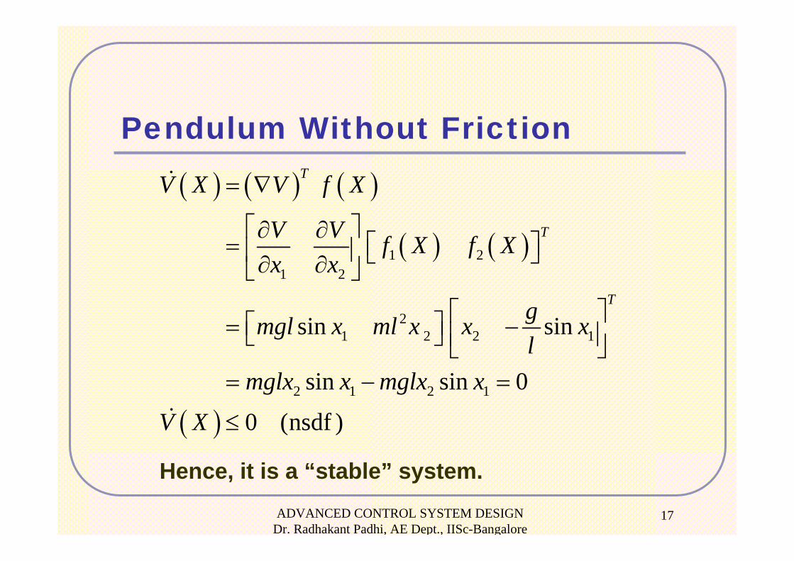
Pendulum Without Friction

( ) ( ) ( )

( ) ( )

( )

1 21 2

21 2 2 1

2 1 2 1

sin sin

sin sin 0

0 (nsdf )

T

T

T

V X V f X

V V f X f Xx x

gmgl x ml x x xl

mglx x mglx x

V X

= ∇

⎡ ⎤∂ ∂= ⎡ ⎤⎢ ⎥ ⎣ ⎦∂ ∂⎣ ⎦

⎡ ⎤⎡ ⎤= −⎣ ⎦ ⎢ ⎥⎣ ⎦= − =

≤

Hence, it is a “stable” system.


18

Pendulum With Friction

Modify the previous example by adding thefriction force

Defining the same state variables as above

θkl

θθ klmgma −−= sin

1 2

2 1 2sin

x xg kx x xl m

=

= − −


19

Pendulum With Friction( ) ( ) ( )

( ) ( )

( ) ( )

1 21 2

21 2 2 1 2

2 22

sin sin

0 nsdf

T

T

T

V X V f X

V V f X f Xx x

g kmgl x ml x x x xl m

kl x

V X

= ∇

⎡ ⎤∂ ∂= ⎡ ⎤⎢ ⎥ ⎣ ⎦∂ ∂⎣ ⎦

⎡ ⎤⎡ ⎤= − −⎣ ⎦ ⎢ ⎥⎣ ⎦= −

≤

Hence, it is also just a “stable” system. (A frustrating result..!)


20

Analysis of Linear Time Invariant System

System dynamics:

Lyapunov function:

Derivative analysis:

, n nX AX A ×= ∈R

( )

T T

T T T

T T

V X PX X PXX A PX X PAX

X A P PA X

= +

= +

= +

( ) ( ), 0 pdfTV X X PX P= >


21


For stability, we aim for

By comparing

For a non-trivial solution

( )T T TX A P PA X X QX+ = −

( )0TV X QX Q= − >

0TPA A P Q+ + =

(Lyapunov Equation)


22


( ) The eigenvalues of a matrix satisfy Re 0 if and only if for any given symmetric matrix , a unique

matrix satisfying the Lyapuno

n ni iA

pdf Q

pdf P

λ λ×∈ <

∃

Theorem :

v equation.

Proof: Please see Marquez book, pp.98-99.

0

and are related to each other by the following relationship:

However, the above equation is seldom used to compute . Instead is directly solved from the Lyapunov equation.

TA t At

P Q

P e Qe dt

P P

∞

= ∫

Note :


23

Analysis of Linear Time Invariant Systems

Choose an arbitrary symmetric positive definite matrix

Solve for the matrix form the Lyapunov equation and verify whether it is positive definite

Result: If is positive definite, then and hence the origin is “asymptotically stable”.

( )Q Q I=

P

P ( ) 0V X <


24

Lyapunov’s Indirect Theorem

( )( )

( )

Let the linearized system about 0 be .

The theorem says that if all the eigenvalues 1, ,

of the matrix satisfy Re 0 (i.e. the linearized systemis exponentially stable), then for t

i

i

X X A X

i n

A

λ

λ

= Δ = Δ

=

<

…

he nonlinear system theorigin is locally exponentially stable.


25

Instability theoremConsider the autonomous dynamical system and assume

is an equilibrium point. Let have thefollowing properties:

Under these conditions, is unstable

( )

( )

0 0

( ) (0) 0( ) ,arbitrarily close to 0, such that 0

( ) 0 , where the set is defined as follows{ : and 0}

n

i Vii X X V X

iii V X U UU X D X V Xε

=

∃ ∈ = >

> ∀ ∈

= ∈ ≤ >

R

0X=

0X=

:V D →R


26

Summary

Motivation

Notions of Stability

Lyapunov Stability Theorems

Stability Analysis of LTI Systems

Instability Theorem

Examples


27

References

H. J. Marquez: Nonlinear Control Systems Analysis and Design, Wiley, 2003.

J-J. E. Slotine and W. Li: Applied Nonlinear Control, Prentice Hall, 1991.

H. K. Khalil: Nonlinear Systems, Prentice Hall, 1996.


28

stability analysis of nonlinear systems using lyapunov ... 31.pdf · nonlinear control, prentice...

Documents