speed and texture: an empirical study on optical-flow accuracy in adas scenarios

136 IEEE TRANSACTIONS ON INTELLIGENT TRANSPORTATION SYSTEMS, VOL. 15, NO. 1, FEBRUARY 2014

Speed and Texture: An Empirical Study onOptical-Flow Accuracy in ADAS Scenarios

Naveen Onkarappa and Angel Domingo Sappa, Senior Member, IEEE

Abstract—Increasing mobility in everyday life has led to theconcern for the safety of automotives and human life. Computervision has become a valuable tool for developing driver assistanceapplications that target such a concern. Many such vision-basedassisting systems rely on motion estimation, where optical flow hasshown its potential. A variational formulation of optical flow thatachieves a dense flow field involves a data term and regularizationterms. Depending on the image sequence, the regularization hasto appropriately be weighted for better accuracy of the flow field.Because a vehicle can be driven in different kinds of environments,roads, and speeds, optical-flow estimation has to be accuratelycomputed in all such scenarios. In this paper, we first presentthe polar representation of optical flow, which is quite suitablefor driving scenarios due to the possibility that it offers to in-dependently update regularization factors in different directionalcomponents. Then, we study the influence of vehicle speed andscene texture on optical-flow accuracy. Furthermore, we analyzethe relationships of these specific characteristics on a drivingscenario (vehicle speed and road texture) with the regularizationweights in optical flow for better accuracy. As required by thework in this paper, we have generated several synthetic sequencesalong with ground-truth flow fields.

Index Terms—Advanced driver assistance systems (ADASs), op-tical flow, regularization parameters, road texture, vehicle speed.

I. INTRODUCTION

THE developments in computer vision and computing sys-tems have drawn the interest of the automotive indus-

try to make use of them toward advanced driver assistancesystems (ADASs). ADASs include lane departure warning,collision avoidance, parking assistance, and autonomous nav-igation (e.g., see [1] and [2]). These systems involve taskssuch as egomotion estimation, moving-object detection, and3-D reconstruction. One of the well-known tools for estimatingmotion that can be used in many of the aforementioned tasksis the optical flow. Optical flow is a displacement vector fieldof patterns between two images. In a driving scenario, opticalflow is estimated between successive video frames captured by

Manuscript received October 3, 2012; revised March 12, 2013, April 29,2013, and July 7, 2013; accepted July 15, 2013. Date of publication August 15,2013; date of current version January 31, 2014. This work was supported inpart by the Spanish Government under Project TIN2011-25606. The work ofN. Onkarappa was supported in part by the Catalan Government through theAgency for Management of University and Research Grants (AGAUR) underan FI Grant. The Associate Editor for this paper was S. S. Nedevschi.

The authors are with the Computer Vision Center, Autonomous Uni-versity of Barcelona, 08193 Barcelona, Spain (e-mail: [email protected];[email protected]).

Color versions of one or more of the figures in this paper are available onlineat http://ieeexplore.ieee.org.

Digital Object Identifier 10.1109/TITS.2013.2274760

a camera that is mounted on a vehicle. The seminal methodsof estimating optical flow were proposed in 1981 in [3] and[4]. The literature shows that there have been several attemptsto improve optical-flow accuracy, with increased interest inrecent years, particularly on variational approaches that typ-ically involve data and regularization terms. The balancingbetween the regularization and data terms has to be tuned toget better flow fields. Almost all the state-of-the-art approachesempirically select this weight for a fixed set of image sets usedfor evaluation.

In the ADAS domain, it can happen that the vehicle is drivenin different environments (e.g., urban, highway, and country-side) [5] with different speeds and different road textures,making it difficult to achieve the same optical-flow accuracy allover the vehicle’s trajectory; in turn, it reduces the confidenceand effectiveness of ADAS applications. It is very importantto adjust the regularization weight based on the environmentwhere the vehicle is being driven. This motivates us in thispaper to analyze the effect of some specific properties of thedriving environment on the optical-flow accuracy. There aremany factors that affect the flow accuracy, such as illumination,occlusions, specularity, texture, structure, and large displace-ments. In particular, in this paper, we study the influence ofonboard vision system speed and also the road texture onoptical-flow accuracy.

As motivated by the natural way of representing a vectorin terms of polar coordinates, it is also demonstrated that thisrepresentation exhibits statistical independence on image se-quences of ADAS scenarios in this paper. The polar-representedoptical-flow estimation [6] involves the following two regular-ization terms: 1) orientation and 2) magnitude. This formulationgives the advantage of independently tuning each term, unlikein Cartesian-represented optical-flow estimation. Fig. 1 showsimage frames of different speeds and textures and the estimatedflow fields based on [6]. The error values [average angularerror (AAE) and average endpoint error (EPE)] for the sameflow fields are given in Table I, where S1 corresponds to thesequence with the lowest speed, whereas S4 corresponds tothe sequence with the highest speed. On the other hand, T1corresponds to the lowest texture contrast, and T3 correspondsto the highest texture contrast. An analysis of errors for a fixedset of regularization weights and different speeds and texturesin both Fig. 1 and Table I reveals the importance of regular-ization weights for an accurate flow-field estimation. In thispaper, we analyze the variation in accuracy of the optical flowby varying the weights of regularization on several sequencesof different speeds and road textures. First, the analysis of theinfluence of just speed is performed. Second, different textures

1524-9050 © 2013 IEEE. Personal use is permitted, but republication/redistribution requires IEEE permission.See http://www.ieee.org/publications_standards/publications/rights/index.html for more information.

ONKARAPPA AND SAPPA: SPEED AND TEXTURE: EMPIRICAL STUDY ON OPTICAL-FLOW ACCURACY IN ADASs 137

Fig. 1. Image frames of different textures and speeds, and computed opticalflows for different regularization weights.

are analyzed. Finally, the analysis that combines both speed andtextural properties is done.

This empirical analysis requires the following image se-quences: 1) to analyze the influence of speed, having sequencesof different speeds with the same geometrical structure andtexture is needed and 2) to analyze the influence of texture,having sequences with the same geometrical scene structurebut with a different texture is needed. It is impossible to havesuch real-life scenarios and also the corresponding ground-truthoptical flow. In this paper, several synthetic sequences of an

TABLE IAAEs AND EPEs FOR FIXED REGULARIZATION WEIGHTS FOR

SEQUENCES OF DIFFERENT TEXTURES AND SPEEDS

(FLOW FIELDS ARE SHOWN IN FIG. 1)

urban scenario for the required cases are rendered using 3-Dmodels that were generated with the graphic editor Maya1; thecorresponding ground-truth flow fields are also generated usinga ray-tracing technique.

In summary, the contributions of this paper are listed asfollows.

1) The statistical independence of polar representation isexploited on ADAS scenarios.

2) The dependency of regularization weights (both for mag-nitude and orientation) are analyzed for different speedsof the onboard vehicle camera, for different road textures,and for different combinations of both speed and texturetogether.

3) Several synthetic sequences of driving scenarios for dif-ferent speeds and different road textures are generatedwith the corresponding ground-truth flow fields.

This paper is organized as follows. The next section presentsthe related work. Then, Section III provides a brief compar-ative study of the use of polar representation with respectto the Cartesian in the context of ADAS applications. Next,Section IV presents the polar optical-flow formulation usedin this paper. The texture measures needed to evaluate thedifferent scenarios are presented in Section V, whereas theframework used to generate scenes is detailed in Section VI.Experimental results, discussions, and conclusions are given inSections VII–IX, respectively.

II. RELATED WORK

Optical-flow techniques can be classified as global and localapproaches. Global approaches produce dense flow fields us-ing variational energy minimization, whereas local approachesproduce sparse flow fields using a least squares criterion oversmall neighborhoods. During the last three decades, severalapproaches on optical-flow estimation have been proposed [7]to improve accuracy and efficiency. Hence, there is a needto evaluate this large amount of contributions. Performanceevaluation of different methods on complex data sets havebeen presented in [8]–[11]. Recently, Baker et al. [12] haveproposed benchmarking sequences with ground-truth data anda methodology for evaluation.

The denseness of global optical-flow approaches make themuseful in many applications. Typically, global optical-flowestimation (e.g., see [13] and [14]) that is formulated as avariational energy minimization consists of a data term thatmatches some properties between images and a smoothnessterm, also called a regularization term, that makes the problem

1www.autodesk.com/maya


well posed. Attempts have been made to improve on data terms,regularization, and energy minimization. Improvements in dataterms are made by robust penalizing functions [15] and byadopting higher order terms [16]. Developments in regulariza-tion terms are focused on preserving motion discontinuities[17] and using the temporal coherence [18]. A method thatcombines the advantages of both local and global approachesis proposed in [16]. Recently, Sun et al. [19] have exploredconcepts such as preprocessing, coarse-to-fine warping, grad-uated nonconvexity, interpolation, derivatives, robustness ofpenalty functions, and median filtering, and then, their influenceon optical-flow accuracy is revealed. Using the best of theexplored concepts and weighted nonlocal median filtering, animproved model is proposed in [19]. A multiframe optical-flowestimation technique based on the temporal coherence of flowvectors across image frames is proposed in [20]. Motivatedby the natural representation of a vector and the statisticalindependence of the polar coordinates to the Cartesian coor-dinates, recently, an optical-flow estimation approach based onpolar representation has been proposed in [6]. A top-performingmethod that intelligently preserves small and large motion in acoarse-to-fine approach is proposed in [21]. In summary, therehas been increased interest on optical-flow approaches in thelast few years, which can be appreciated on the number ofpublications and released code [11].

We can notice that, in almost all optical-flow methods, theweights for regularization are empirically chosen. There arevery few attempts in this direction to automatically select suchparameters. Krajsek et al. [22] present a Bayesian model thatautomatically weighs different data terms and a regulariza-tion term. This model that estimates optical flow and severalparameters together is very complex to minimize. Recently,Zimmer et al. [23] has proposed to automatically select theregularization weight based on the optimal prediction principle.In their work, the optimal regularization weight is obtainedas the one that can produce a flow field with which the nextframe in a sequence is best predicted. Inherently, this approachinvolves a brute-force method to select the optimal weightbased on the average data constancy error, and hence, it iscomputationally expensive. On the other hand, there is anattempt [24] to use several different optical-flow methods fora sequence by selecting the best suitable method per pair offrames or per pixel.

In a preliminary work [25], we present a study on optical-flow accuracy for different speeds of the vehicle. In that work,the size of the video sequence is very small, and the framesconsidered for speed analysis involve a different geometricalscene structure. In this paper, in particular, the study on speedis improved by adding longer sequences. In addition, boththe study of texture and the combined study on speed andtexture have been performed on sequences that include complexscenarios.

III. POLAR VERSUS CARTESIAN REPRESENTATION

OF FLOW VECTORS

The most commonly used representation in optical-flow esti-mation is the Cartesian coordinate system. However, represent-

Fig. 2. Joint histograms of flow derivatives in the Cartesian and polar coor-dinates of an estimated flow field in a synthetic sequence of an urban roadscenario. On top of each plot, the MI value is depicted.

ing a vector in terms of its magnitude and orientation is a naturalway that is referred to as polar representation. As presentedin [6], the analysis of spatial derivatives distribution of a flowfield represented in polar shows a significant statistical differ-ence among its components compared to the components ofa Cartesian representation. Furthermore, the polar componentsshow higher statistical independence compared to the Cartesiancomponents when the mutual information (MI) between thederivatives of flow components in the respective representationsare analyzed, as shown in [6] and [26].

A similar analysis is shown in Fig. 2. This analysis is per-formed on the estimated optical-flow field from a pair of imagesin an urban driving scenario (shown in Fig. 3, left column).Fig. 2 shows the joint histograms of flow derivatives in both theCartesian and polar coordinate systems. The MI between thecoordinate components that were computed using these jointhistograms are depicted on top of each plot in Fig. 2. The lowerthe values of MI, the higher the statistical independence. Asshown in Fig. 2, the representation of flow field in polar is moreindependent than the Cartesian system. A similar analysis onthe ground-truth flow field between the same pair of images hasshown zero MI (in the cases in Fig. 2, bottom left and bottomright), for polar coordinates. For the Cartesian coordinates (inthe cases in Fig. 2, top left and top right), the MI valuesare 0.27082 and 0.50335, respectively, when the ground-truthflow field is considered. This shows that, in the ideal case oftranslational motion, polar coordinates are mutually exclusive(totally independent).

A polar representation of flow vectors for optical-flow esti-mation is proposed in [6], and its implications are studied. Itis shown that polar-represented optical flow performs almost


Fig. 3. Images from sequences of different speeds. Top left: First framecommon for all sequences. Top right: Color map used to show the flow fields.Left column: Second frame from the sequences of different speeds in increasingorder (second and third rows). Right column: Ground-truth flow fields betweenthe respective first and second frames.

similar to the state-of-the-art Cartesian coordinates representedoptical-flow estimation on traditional image data sets. Fur-thermore, it is shown that, for specular and fluid flow imagesets, polar representation adds the advantage by independentlyallowing regularization in either coordinate component. In thevehicle-driving scenario, the majority of the motion is transla-tion. The expected flow field in such a scenario is diverging, andthe variation in magnitude is higher compared to the variationin orientation. In such a motion scenario, the polar opticalflow becomes convenient. This paper exploits the possibility ofindependent tuning of regularization terms.

IV. OVERVIEW OF THE POLAR OPTICAL FLOW

A typical variational formulation of the optical-flow energyfunction using the Cartesian representation looks like

E(u, v) =

∫ ∫Ω

⎧⎨⎩(I(x+ u, y + v, t+ 1)− I(x, y, t))︸︷︷︸

DataTerm

+ α(|∇u1|2 + |∇u2|2

)︸︷︷︸

Regularization

⎫⎪⎬⎪⎭ dx dy, (1)

which contains a data and a regularization term. Here, I(x, y, t)is the pixel intensity value at (x, y) at time t, α is the reg-ularization weight, and (u, v) is the flow-field vector to be

estimated using Euler–Lagrange equations [14] or alternativemethods [13].

This section presents a brief description of the polar optical-flow formulation proposed in [6]. According to that work, theflow vector at a pixel (x, y) can be represented in terms of polarcoordinates as

flow(x, y) = (m(x, y), θ(x, y)) (2)

where m is the magnitude, and θ is the orientation at (x, y). Theenergy formulation using the polar representation allows us toseparate the regularization terms as follows:

E (θ(x, y),m(x, y))

=

∫ ∫Ω

{ψ (I(x+m cos θ, y +m sin θ, t+ 1)− I(x, y, t))

+ αθψθ (ρθ(θ)) + αmψm (ρm(m))} dx dy, (3)

where ψ is a robust penalty function for the data term, andψθ and ψm are robust penalty functions, respectively, for theorientation and magnitude components’ regularization (see [6]for more details). Similarly, αθ and αm are regularizationweights, and ρθ and ρm are differential operators (in a simplercase, the first derivative). All these ρ∗, ψ∗, and α∗ can be varied,depending on the image sequences or application of interest.

To avoid the difficulty of m being negative, the followingequivalence relation is defined over values of m and θ:

(m, θ) ∼{(m, θ) if m > 0(−m, θ + π) if m < 0.

(4)

Due to the periodic nature of θ, the orientation is expressedin terms of two parameters as

s(x, y) = sin θ(x, y)

c(x, y) = cos θ(x, y) (5)

where the constraint s2 + c2 = 1 is called the coherence con-straint, which ensures proper representation of orientation.

Using the Lagrange multiplier λ and assuming that it as a pre-determined parameter, the energy function can be formulated tominimize three parameters (c, s,m) as

E(c, s,m)

=

∫ ∫Ω

{λ(s2 + c2 − 1)2

+ ψ (I(x+mc, y +ms, t+ 1)− I(x, y, t))

+ αθψθ (ρθ(c), ρθ(s))+αmψm (ρm(m))} dx dy,

(6)

where λ is a pixelwise predetermined parameter that is updatedevery iteration as λ = e(s

2+c2−1)2 using the previous itera-tion values of c and s. Equation (6) can be minimized usingEuler–Lagrange equations.


V. TEXTURE MEASURES

To study the effect of texture on optical-flow accuracy, it isnecessary to quantify the texture property. There are severalways of measuring the texture content of a given sequence[27]; in this paper, three of the most widely used statisticaltexture metrics, i.e., contrast, correlation, and homogeneity,are considered. These metric values are computed over a co-occurrence matrix of gray values of images [28] and arecorrelated with the optical-flow error measures. The texturemetrics computed over the co-occurrence matrix, which is alsocalled normalized gray-level co-occurrence matrix (GLCM) ofan image, are defined as

Contrast =

Ng−1∑n=0

n2

⎧⎨⎩

Ng∑i=1

Ng∑j=1

p(i, j)

⎫⎬⎭ ; |i− j| = n

(7)

Correlation =

∑Ng

i=1

∑Ng

j=1(ij)p(i, j)− μxμy

σxσy(8)

Homogeneity =

Ng∑i=1

Ng∑j=1

p(i, j)

1 + |i− j| (9)

where p(i, j) is the (i, j)th entry in the normalized GLCM, Ng

is the number of distinct gray levels in the quantized image, andμx, μy , σx, and σy are the means and standard deviations of pxand py: px(i) =

∑Ng

j=1 p(i, j), and py(j) =∑Ng

i=1 p(i, j).

VI. SYNTHETIC SEQUENCE GENERATION FRAMEWORK

To analyze the influence of speed on optical-flow accuracy,we need to have image sequences of the same scene, but withthe onboard vision system moving with different speeds onexactly the same trajectory. Similarly, to analyze the impactof texture, we need image sequences of the same scene (i.e.,surrounding scene structure) but with just different textures. Inreality, it is impossible to have such scenarios and to gener-ate ground-truth optical flow. Although it is possible to havesuch sequences in a controlled laboratory environment, theredoes not exist any sensor to generate ground-truth flow fields.The only way to have such scenarios is to build virtual 3-Dmodels and use them in the aforementioned setup (speed andtexture). In fact, there are several data sets available withground-truth in the literature (e.g., [12], [29], and [30]). In[12], different synthetic and real data sets for general motionscenarios with the ground truth are presented, whereas in [29],many synthetic sequences with the ground truth for ADASscenarios are presented. The work presented in [30] providessynthetic sequences of varied complexities that were createdusing the open movie Sintel as a benchmark in optical-flowresearch. Recently, [31] has proposed a data set (KITTI) of realsequences with ground-truth flow in ADAS scenarios. AlthoughKITTI has real sequences of ADAS scenarios, it does notcontain sequences for studying the influence of speed/texture.In summary, none of the available data sets are suitable for thestudy proposed in this paper. Mac Aodha et al. in [24] presented

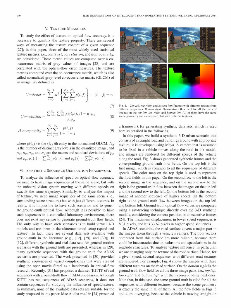
Fig. 4. Top left, top right, and bottom left: Frames with different texture fromdifferent sequences. Bottom right: Ground-truth flow field for all the pairs ofimages on the top left, top right, and bottom left. All of them have the samescene geometry and same speed, but with different textures.

a framework for generating synthetic data sets, which is usedhere as detailed in the following.

In this paper, we build a synthetic 3-D urban scenario thatconsists of a straight road and buildings around with appropriatetexture; it is developed using Maya. A camera that is assumedto be fixed in a vehicle moves along the road in the model,and images are rendered for different speeds of the vehiclealong the road. Fig. 3 shows generated synthetic frames and thecorresponding ground-truth flow fields. On the top left is thefirst image, which is common to all the sequences of differentspeeds. The color map on the top right is used to representthe flow fields in this paper. On the second row to the left is thesecond image in the sequence, and on the second row to theright is the ground-truth flow between the images on the top leftand the second row to the left. On the bottom left is the secondimage of another sequence of higher speed. On the bottomright is the ground-truth flow between images on the top leftand bottom left. Ground-truth optical-flow values are computedusing a ray-tracing technique directly over the 3-D syntheticmodels, considering the camera position in consecutive frames[24]. The maximum displacement in lower speed sequences is8.31 pixels, and it is 33.67 pixels in higher speed sequences.

In ADAS scenarios, the road surface covers a major part inthe images taken through a vehicle’s camera. The flow vectorscomputed from this surface are more reliable, because therecould be inaccuracies due to occlusions and specularities in theroadside structures. To analyze texture influence, in particular,we are changing only the texture of the road surface. Hence, fora given speed, several sequences with different road texturesare rendered. For example, Fig. 4 shows the images with threedifferent textures on the road surface. On the bottom right is theground-truth flow field for all the three image pairs, i.e., top left,top right, and bottom left, with their corresponding next ones.Note that, in this case, the same ground truth is valid for all thesequences with different textures, because the scene geometryis exactly the same in all of them. All the flow fields in Figs. 3and 4 are diverging, because the vehicle is moving straight on


Fig. 5. Top: Two different image frames from a sequence with independentlymoving vehicles and different egomotion. Bottom: Ground-truth flow fieldsbetween the top frames and to their next ones in the sequence.

a road. In addition to these sequence sets, which are simplein motion, we have created another set of complex sequencesfor different speeds and textures similar to the previous set ofsequences. The new complex sequences contain two movingvehicles: one vehicle moves along the road and comes towardthe onboard camera vehicle, and the other vehicle comes froma cross road toward the onboard camera vehicle. The newsequences also contain changes in yaw and pitch angles duringthe vehicle’s trajectory. The yaw is 0.25◦ to the left/right, andthe pitch is 0.25◦ to the up/down. Two of the image framesfrom this new sequence and the ground-truth optical flows withtheir next image frames are shown in Fig. 5. All the renderedimages are of a resolution of 480 × 640 pixels, and the camerafocal length is 35 mm. All this data set (i.e., rendered framesfor different video sequences and corresponding ground-truthflows) is available through our website.2

VII. EXPERIMENTAL ANALYSIS

This section presents the empirical study of the optical-flowaccuracy of scenes, where the following conditions hold: 1) thecamera moves at different speeds; 2) the texture of the scenechanges; and 3) both speed and texture changes are consideredtogether. First, we perform the study for all these three caseson a set of simple sequences, where there is no complexity, andthe vehicle’s camera moves straight on a road with differentspeeds and with different road textures. Such a simple sequenceenables us to easily analyze the influence of speed and textures.Then, we also present the study of the influence of speed andtexture together with another set of sequences that has complexegomotion.

A. Analysis for Speed

Following the framework presented in Section VI, we havegenerated four sequences of different speeds with an incremen-tal translation of 0.25, 0.5, 0.75, and 1 cm along the optical

2http://www.cvc.uab.es/adas

Fig. 6. RoIs used to calculate the error measures. Left: Speed analysis. Right:Texture, and speed together with texture analysis.

Fig. 7. Three-dimensional plot of the AAEs from S1 for varying αθ and αm

values.

axis of the vehicle camera in a Maya model with a workingunit as centimeter. Let us call these sequences S1, S2, S3,and S4 in increasing order of speed. The ground-truth opticalflows for these sequences are also generated. The scene andtexture of all these sequences are shown in Fig. 3. The firstaim is to study optical-flow accuracy for the change in speedand to find its relationship with respect to the regularizationparameters in the optical-flow formulation. We use the polaroptical flow presented in Section IV, because this formulationprovides the possibility of separately tuning different regular-ization parameters, which is an attractive feature in the ADASdomain. Furthermore, it involves two regularization terms thatallow an independent study of their influence. Initially, ex-perimentation is performed to find the optimal range for theregularization weights. It consists of computing optical flowon a pair of images from one of the sequences for a widerange of weights of both regularization terms. Based on thisexperiment, it is determined that the following range of valuesfor experimentation is sufficient: 1, 2.5, 5, 10, 20, 30, . . ., 120.


Fig. 8. Three-dimensional plot of the AAEs of all sequences for varying αθ

and αm values.

Further, for analysis of the influence of speed, it is not goodto have an equal number of frames in all of the sequencesof different speeds. Because each sequence has a differentdisplacement per frame, having an equal number of frames inall of them will result in having the vehicle camera move dif-ferent distances and ending up processing different sequences.Because there is a different scene geometry with differentbuildings in the 3-D model, the nth frame in S1 will have adifferent scene geometry from the nth frame in S2, S3, and S4.Because the scene geometry also affects optical-flow accuracy,in this experiment, we have generated sequences of differentspeeds, but the vehicle camera travels a constant distance inall of them along the camera axis of the 3-D model, hencegenerating varying numbers of frames in different sequences.This way, all the sequences cover exactly the same geometricscene, but with a different number of frames. Therefore, wehave 40 frames in S1, 20 frames in S2, 13 frames in S3, and 10frames in S4. The average of error measures of all the framesin a sequence are considered for analysis. We have consideredboth AAE and EPE for analysis. All the errors in this analysisare computed over a region of interest (RoI) of size 320 × 480at the center of the flow field. The considered RoI is shown inFig. 6, left.

Fig. 7 shows a 3-D representation of the AAE for sequenceS1 for varying values of two regularization weights αθ andαm. The 3-D error representations of AAEs from all the foursequences are shown in Fig. 8. The minimum AAEs and thecorresponding regularization weights for all the sequences aregiven in Table II. Observing the meshes in Fig. 8 and by ana-lyzing the minimum AAE values in Table II, we can concludethat the error in the sequence of lower speed is always higherthan the error in the sequence of higher speed at almost allcombinations of regularization weights. The values of αθ andαm in Table II reveal that αθ is constant around 2.5 and 5, whereαm values decrease as the speed increases. It can be inferredthat, overall, the AAE decreases with the increase in speed ofthe vehicle, αθ has to slightly be increased, and αm should betuned with the change in speed of the vehicle.

TABLE IIREGULARIZATION PARAMETER VALUES THAT PRODUCE THE

LOWEST AAEs IN EACH OF THE SEQUENCES

Fig. 9. Three-dimensional plot of the EPEs from S1 for varying αθ and αm

values.

Fig. 10. Three-dimensional plot of the EPEs of all sequences for varying αθ

and αm values.

A similar analysis is also done using the EPE. Fig. 9 showsthe 3-D representation of the EPE for S1 for all combinationsof two regularization weights. The 3-D representations of EPEsof all four sequences are depicted in Fig. 10. The minimumEPEs for all four sequences with corresponding regularizationweights are shown in Table III. It is observed in the errormaps in Fig. 10 and Table III that the EPE in a lower speedsequence is lower than in a sequence of higher speed for anycombination of both regularization weights. In Table III, αθ

increases from a smaller value as the speed increases, whereas


TABLE IIIREGULARIZATION PARAMETER VALUES THAT PRODUCE THE

LOWEST EPEs IN EACH OF THE SEQUENCES

TABLE IVTEXTURE METRICS FOR THE DIFFERENT SEQUENCES

αm keeps constant at around value 60. From the point ofview of EPE, αm has to be kept constant at a higher value,and αθ should be tuned according to the change in speed ofthe vehicle. One interesting conclusion from this first studyis that, depending on the required accuracy (AAE or EPE,i.e., angular or magnitudinal) needed for a given application,different tuning of regularization parameters has to be applied.Furthermore, it is clear that there is a relationship between thisparameter tuning and the current speed of the vehicle.

B. Analysis for Texture

The aim of the work in this section is to analyze the influenceof road texture on optical-flow accuracy and to identify theway of adjusting the regularization weights for better results.We have generated several sequences with different road tex-tures, and some of the images of these sequences are shownin Fig. 4. The study in this section is performed consideringthree sequences with the increasing value of texture contrast.Hereinafter, they are referred to as T1, T2, and T3. Thesesequences are of the same speed as S1, but with different roadtextures. The texture metrics are computed over a small RoIof size 146 × 430 on the road surface. This RoI is shownin Fig. 6, right. Again, in this section, the polar-representedoptical flow described in Section IV is used. The optical flowis computed on all image pairs from these sequences, whichwere obtained by assuming that the onboard vision systemtravels at the same speed. The average error values of all theflow fields in the same small RoI (where texture metrics werecalculated) in a sequence are computed. We consider both theAAE and EPE for analysis. Table IV gives the texture metricsfor the sequences. Figs. 11 and 12 show 3-D representationsof AAEs and EPEs, respectively, for three sequences of differ-ent textures T1, T2, and T3. The minimum AAEs and EPEswith the corresponding regularization weights are shown inTables V and VI, respectively. By observing Figs. 11 and 12and Tables V and VI, it can easily be confirmed that boththe AAE and EPE measures decrease with the increase intexture contrast. The regularization weights in Tables V andVI reveal that both values should increase with the increase intexture contrast for better results. Similarly, these results canbe correlated with other textural properties such as correlationand homogeneity in Table IV.

Fig. 11. Three-dimensional plot of the AAEs from three different texturedsequences for varying αθ and αm values.

Fig. 12. Three-dimensional plot of the EPEs from three different texturedsequences for varying αθ and αm values.

TABLE VREGULARIZATION PARAMETER VALUES WITH THE LOWEST AAEs

TABLE VIREGULARIZATION PARAMETER VALUES WITH THE LOWEST EPEs

C. Analysis for Both Speed and Texture

Furthermore, we have performed experiments to analyzethe influences of both speed and texture together. We use 12different sequences of four different speeds and three differenttextures. Optical flow is estimated on all the frames in these


Fig. 13. Error images for the same image pairs shown in Fig. 1 and Table I.Left: AAEs. Right: EPEs.

sequences, and errors are computed. The error for a particularsequence is the average of errors in all the flow fields in that se-quence. Error heat maps are shown in Fig. 13 for the same flowfields shown in Fig. 1. The errors are calculated on a small RoIof size 146 × 430 on the road surface, which is the same as inthe previous subsection. Table VII shows the minimum AAEs

TABLE VIIMINIMUM AAEs AND THEIR CORRESPONDING

REGULARIZATION WEIGHTS (αθ, αm)

Fig. 14. Three-dimensional plot of the minimum AAE for all sequences withdifferent speeds and textures for varying αθ and αm values.

Fig. 15. Three-dimensional plot of αθ that corresponds to the minimum AAEfor all sequences with different speeds and textures.

for 12 different sequences of different speeds and textures. Theregularization weights that correspond to the minimum errorsare also mentioned in brackets in Table VII. Three-dimensionalplots of the minimum AAEs and the corresponding αθ’s andαm’s are shown in Figs. 14–16, respectively. In Table VII andFig. 14, we can notice that the AAE reduces with the increasein texture contrast, as well as with the increase in speed.With respect to the AAE, Fig. 15 indicates that αθ has to bekept small and slightly increase when the speed increases for asequence of lower texture, but it has to be higher and to increase


Fig. 16. Three-dimensional plot of αm that corresponds to the minimumAAE for all sequences with different speeds and textures.

TABLE VIIIMINIMUM EPEs AND THEIR CORRESPONDING


Fig. 17. Three-dimensional plot of the minimum EPE for all sequences withdifferent speeds and textures for varying αθ and αm values.

when the speed increases for a sequence of higher texture. Inconclusion, αθ has to increase with the increase in speed andtexture. The 3-D representation in Fig. 16 indicates that αm hasto decrease with the increase in speed and to increase with theincrease in texture.

A similar experiment on all the 12 sequences is performedconsidering the EPEs. Table VIII shows the minimum EPEsand the corresponding regularization weights in brackets.Figs. 17–19 are the 3-D representations of the minimum EPEs,αθ’s, and αm’s, respectively. In Table VIII and Fig. 17, we

Fig. 18. Three-dimensional plot of αθ that corresponds to the minimum EPEfor all sequences with different speeds and textures.

Fig. 19. Three-dimensional plot of αm that corresponds to the minimum EPEfor all sequences with different speeds and textures.

can observe that the EPE reduces with the increase in texturecontrast but increases with the increase in speed. Fig. 18 showsthat αθ has to increase with the increase in speed and with theincrease in texture contrast, whereas the 3-D representation inFig. 19 indicates that αm has to increase with the increase intexture but has to decrease with the increase in speed, exceptfor lower textured sequences (e.g., the sequence with textureT1 and with speeds S1, S2, S3, and S4).

Furthermore, to ensure the conclusions based on Tables IIand VII about the decrease in AAE with the increase in speedand the conclusion that the AAE will decrease with the increasein texture contrast, we analyzed the AAEs of all 12 sequences,keeping αθ and αm constant at different values. Table IX showsthe AAEs in all sequences for fixed αθ and αm values at 40.The AAEs in this table confirm our conclusion that the AAEdecreases with the increase in speed and texture. Comparingthe error values in Tables VII and IX, it is clear that tuningof regularization weights is very important in getting accurateoptical flow. Similarly, Table X shows the EPEs for a fixedαθ and αm value of 40 for the sequences. This also reaffirmsthat the EPE increases with the increase in speed but decreases


TABLE IXAAEs FOR FIXED REGULARIZATION WEIGHTS: αθ = 40 AND αm = 40

TABLE XEPEs FOR FIXED REGULARIZATION WEIGHTS: αθ = 40 AND αm = 40

with the increase in texture and comparing values based onTables VIII and X reveals that tuning of regularization weightsis needed.

Finally, a similar analysis as in the previous one has beenperformed, but by adding complexity to the motion. The newsequences involve large changes in (yaw and pitch) angles.All these sequences are ten frames long. The optical flow iscomputed for varying regularization weights, and the errorsare computed on a small RoI (the one shown in Fig. 6, right).The minimum AAE and EPE are shown in Tables XI and XII,respectively, for all the 12 different sequences in this complexset. All these sequences have the same degree of egomotion, butthe onboard camera moves at different speeds and on differenttextures. Here, we can observe almost the same trends in errorvalues and regularization weights as in the previous study. αθ

has to be increased when the speed and texture contrast increasefor both the AAE and EPE, whereas αm has to be increasedwhen the texture contrast increases for both the AAE and EPE.Because sequences have egomotion, changes in αm do notaffect much in the AAE; it is almost constant with the increasein speed for the AAE, and it has to slightly decrease with theincrease in speed for the EPE.

For the completeness of our study, we have added fewindependently moving vehicles in the scene and performedsimilar analysis. In this particular case, the RoI correspondsto the one shown in Fig. 6, left. As expected, independentlymoving objects are another source of errors that cannot betackled merely by tuning regularization weights, although itcould improve. The relative motion of onboard camera andmoving vehicles causes different groups of flow vectors. Errorsdue to occlusions and due to moving objects present in the sceneare not under our control by tuning regularization weights.Overall, we can tune on the things that are related with staticand under our control (such as speed and texture), but not onthe behavior of dynamic moving vehicles present in the givenscenario.

VIII. DISCUSSION

Although it is out of the scope of this paper the question onhow we can tune the regularization parameters could arise. Ingeneral, based on the aforementioned study, we can say thathaving the best set of parameters would depend on the current

TABLE XIMINIMUM AAEs AND THEIR CORRESPONDING


TABLE XIIMINIMUM EPEs AND THEIR CORRESPONDING


scenario; however, for a given set of regularization parameters(independently, whether it is the best set), we can adapt itsvalues according to the speed and texture using the informationpresented in the previous section. We perceive that this analysisis just a tip on how to proceed and a rigorous study and valida-tion should be performed to define a rule to adapt regularizationparameters to particular characteristics of a sequence. A muchdeeper study is required to conclude adaptation rules in the caseof combinations of several characteristics of any sequence. Thestudy in this paper is a starting point in that direction.

Although an increase in speed of the vehicle camera can becompensated for by increasing the camera cycle time, which isby a higher number of frames per second (FPS), the increasein the number of frames leads to higher computation burden.A related work [32] in that direction proposes to change theresolution of images for varied FPS in a variational hierarchicalframework. Moreover, the maximum number of FPS of acamera is limited by its hardware. In this paper, the influence ofvehicle speed for a fixed cycle time of a camera is considered.

IX. CONCLUSION

This paper has shown that the polar representation of flowvectors is very convenient in ADAS scenarios due to itsfreedom of differently weighing regularization terms and hasfurther used polar-represented optical-flow estimation for theanalysis. The analysis of optical-flow accuracy to specific char-acteristics of a driving scenario, e.g., vehicle speed and roadtexture, is performed. It is concluded that there is a need totune the regularization parameters, depending on the neededaccuracy (angular or magnitudinal) and for varying speeds andtextural properties of the road. This paper has also presented aframework and generated synthetic video sequences along withground-truth flow fields for different scenarios of speeds androad textures.


REFERENCES

[1] A. Jazayeri, H. Cai, J. Y. Zheng, and M. Tuceryan, “Vehicle detection andtracking in car video based on motion model,” IEEE Trans. Intell. Transp.Syst., vol. 12, no. 2, pp. 583–595, Jun. 2011.

[2] S. Cherng, C.-Y. Fang, C.-P. Chen, and S.-W. Chen, “Critical motiondetection of nearby moving vehicles in a vision-based driver-assistancesystem,” IEEE Trans. Intell. Transp. Syst., vol. 10, no. 1, pp. 70–82,Mar. 2009.

[3] B. K. P. Horn and B. G. Schunk, “Determining optical flow,” Artif. Intell.,vol. 17, no. 1–3, pp. 185–203, Aug. 1981.

[4] B. D. Lucas and T. Kanade, “An iterative image registration techniquewith an application to stereo vision (DARPA),” in Proc. DARPA ImageUnderstanding Workshop, Apr. 1981, pp. 121–130.

[5] I. Tang and T. P. Breckon, “Automatic road environment classifica-tion,” IEEE Trans. Intell. Transp. Syst., vol. 12, no. 2, pp. 476–484,Jun. 2011.

[6] Y. Adato, T. Zickler, and O. Ben-Shahar, “A polar representation ofmotion and implications for optical flow,” in Proc. IEEE Conf. Comput.Vis. Pattern Recognit., Colorado Springs, CO, USA, Jun. 2011, pp. 1145–1152.

[7] A. Bruhn, “Variational optic flow computation: Accurate modeling and ef-ficient numerics,” Ph.D. dissertation, Dept. Math. Comput. Sci., SaarlandUniv., Saarbrücken, Germany, 2006.

[8] J. L. Barron, D. J. Fleet, and S. S. Beauchemin, “Performance of opticalflow techniques,” Int. J. Comput. Vis., vol. 12, no. 1, pp. 43–77, Feb. 1994.

[9] B. Galvin, B. Mccane, K. Novins, D. Mason, and S. Mills, “Recoveringmotion fields: An evaluation of eight optical flow algorithms,” in Proc.British Mach. Vis. Conf., Southampton, U.K., 1998, pp. 195–204.

[10] M. Otte and H.-H. Nagel, “Estimation of optical flow based on higherorder spatiotemporal derivatives in interlaced and noninterlaced imagesequences,” Artif. Intell., vol. 78, no. 1/2, pp. 5–43, Oct. 1995.

[11] [Online]. Available: http://vision.middlebury.edu/flow/[12] S. Baker, D. Scharstein, J. P. Lewis, S. Roth, M. J. Black, and R. Szeliski,

“A database and evaluation methodology for optical flow,” Int. J. Comput.Vis., vol. 92, no. 1, pp. 1–31, Mar. 2011.

[13] A. Wedel, T. Pock, C. Zach, D. Cremers, and H. Bischof, “An improvedalgorithm for TV-L1 optical flow,” in Proc. Dagstuhl Motion Workshop,Dagstuhl Castle, Germany, Sep. 2008, pp. 23–45.

[14] T. Brox, A. Bruhn, N. Papenberg, and J. Weickert, “High-accuracy opticalflow estimation based on a theory for warping,” in Proc. Eur. Conf.Comput. Vis., Prague, Czech Republic, May 2004, vol. 3024, pp. 25–36.

[15] M. Black and P. Anandan, “Robust dynamic motion estimation over time,”in Proc. IEEE Conf. Comput. Vis. Pattern Recognit., Maui, HI, USA, Jun.1991, pp. 296–302.

[16] A. Bruhn, J. Weickert, and C. Schnörr, “Lucas/Kanade meets Horn/Schunck: Combining local and global optic flow methods,” Int. J. Comput.Vis., vol. 61, no. 3, pp. 211–231, Feb. 2005.

[17] H.-H. Nagel and W. Enkelmann, “An investigation of smoothness con-straints for the estimation of displacement vector fields from image se-quences,” IEEE Trans. Pattern Anal. Mach. Intell., vol. PAMI-8, no. 5,pp. 565–593, Sep. 1986.

[18] J. Weickert and C. Schnörr, “Variational optic flow computation with aspatiotemporal smoothness constraint,” J. Math. Imaging Vis., vol. 14,no. 3, pp. 245–255, May 2001.

[19] D. Sun, S. Roth, and M. J. Black, “Secrets of optical flow estimation andtheir principles,” in Proc. IEEE Conf. Comput. Vis. Pattern Recognit., SanFrancisco, CA, USA, Jun. 2010, pp. 2432–2439.

[20] S. Volz, A. Bruhn, L. Valgaerts, and H. Zimmer, “Modeling tempo-ral coherence for optical flow,” in Proc. IEEE Int. Conf. Comput. Vis.,Barcelona, Spain, Nov. 2011, pp. 1116–1123.

[21] L. Xu, J. Jia, and Y. Matsushita, “Motion detail preserving optical flowestimation,” IEEE Trans. Pattern Anal. Mach. Intell., vol. 34, no. 9,pp. 1744–1757, Sep. 2012.

[22] K. Krajsek and R. Mester, “Bayesian model selection for optical flowestimation,” in Proc. DAGM Symp., Heidelberg, Germany, Sep. 2007,pp. 142–151.

[23] H. Zimmer, A. Bruhn, and J. Weickert, “Optic flow in harmony,” Int. J.Comput. Vis., vol. 93, no. 3, pp. 368–388, Jul. 2011.

[24] O. Mac Aodha, G. J. Brostow, and M. Pollefeys, “Segmenting videointo classes of algorithm—Suitability,” in Proc. IEEE Conf. Comput. Vis.Pattern Recognit., San Francisco, CA, USA, Jun. 2010, pp. 1054–1061.

[25] N. Onkarappa and A. Sappa, “An empirical study on optical flow accuracydepending on vehicle speed,” in Proc. IEEE Intell. Veh. Symp., Jun. 2012,pp. 1138–1143.

[26] S. Roth and M. J. Black, “On the spatial statistics of optical flow,” in Proc.IEEE Int. Conf. Comput. Vis., Beijing, China, Oct. 2005, pp. 42–49.

[27] P. Wu, Y. M. Ro, C. S. Won, and Y. Choi, “Texture descriptors inMPEG-7,” in Proc. Int. Conf. Comput. Anal. Images Patterns, Warsaw,Poland, Sep. 2001, pp. 21–28.

[28] R. M. Haralick, K. Shanmugam, and I. Dinstein, “Textural features forimage classification,” IEEE Trans. Syst., Man Cybern., vol. SMC-3, no. 6,pp. 610–621, Nov. 1973.

[29] T. Vaudrey, C. Rabe, R. Klette, and J. Milburn, “Differences betweenstereo and motion behavior on synthetic and real-world stereo sequences,”in Proc. Image Vis. Comput., Christchurch, New Zealand, Nov. 2008,pp. 1–6.

[30] D. J. Butler, J. Wulff, G. B. Stanley, and M. J. Black, “A naturalistic opensource movie for optical flow evaluation,” in Proc. Eur. Conf. Comput.Vision, A. Fitzgibbon, P. Perona, Y. Sato, and C. Schmid, Eds., Oct. 2012,pp. 611–625, Springer-Verlag.

[31] A. Geiger, P. Lenz, and R. Urtasun, “Are we ready for autonomous driv-ing? The KITTI Vision Benchmark Suite,” in Proc. IEEE Comput. Vis.Pattern Recognit., Providence, RI, USA, Jun. 2012, pp. 3354–3361.

[32] Y. Kameda, A. Imiya, and T. Sakai, “Hierarchical properties of multireso-lution optical flow computation,” in Proc. ECCV Workshops Demo., 2012,vol. 7584, pp. 576–585, Springer Berlin Heidelberg.

Naveen Onkarappa received the B.Sc. degreein computer science from Kuvempu University,Shimoga, India, in 1999 and the M.Sc. degree incomputer science and the M.Sc.Tech. degree (byresearch) in computer science and technology fromthe University of Mysore, Mysore, India, in 2001 and2007, respectively. He is currently a Ph.D. student,under the supervision of Dr. Angel D. Sappa, at theComputer Vision Center, Autonomous University ofBarcelona, Barcelona, Spain.

From 2001 to 2005, he was a Guest Lecturer withKuvempu University and the University of Mysore. From 2007 to 2009 he waswith HCL Technologies, Bangalore, India. He is a member of the AdvancedDriver Assistance Systems Group, Computer Vision Center, Autonomous Uni-versity of Barcelona. His research interests include optical-flow estimation andits applications to driver assistance systems.

Angel Domingo Sappa (S’94–M’00–SM’12) re-ceived the B.Eng. degree in electromechanical engi-neering from the National University of La Pampa,General Pico, Argentina, in 1995 and the Ph.D. de-gree in industrial engineering from the PolytechnicUniversity of Catalonia, Barcelona, Spain, in 1999.

In 2003, after holding research positions in France,the U.K., and Greece, he joined the Computer Vi-sion Center, Autonomous University of Barcelona,Barcelona, Spain, where he is currently a SeniorResearcher. He is a member of the Advanced Driver

Assistance Systems Group, Computer Vision Center, Autonomous Universityof Barcelona. His research interests include 2-D and 3-D image processing,with emphasis on stereoimage processing and analysis, 3-D modeling, denseoptical-flow estimation, and visual SLAM for driving assistance.

speed and texture: an empirical study on optical-flow accuracy in adas scenarios

Documents