some class-participation demonstrations for introductory ...€¦ · courses in probability and...

Journal of Educational and Behavioral Statistics Spring 2000, Vol. 25, No. 1, pp. 84-100

Some Class-Participation Demonstrations for Introductory Probability and Statistics

Andrew Gelman Columbia University

Mark E. Glickman Boston University

Keywords: classroom activities, conditional probability, confidence intervals, experimentation, hypotheses testing, instruction, numeracy, sampling distributions

We present several classroom demonstratiott~, based on well-known statistical ideas, that have sparked student involvement in our introductory undergraduate courses in probability and statistics.

Most statistics courses at the college (or high school) level, whether con- ducted in departments of statistics, mathematics, psychology, or elsewhere, are taken as a requirement by students who, unfortunately, often have little interest in the subject. There are several excellent textbooks at this level, and lecture time is often used to present examples--including realistic applications of statistics and also simplified examples to clarify the key issues that are covered in the text and homeworks. We have found that the simplified examples can be effectively taught by involving students in participatory demonstrations, rather than the instructor merely lecturing at the blackboard. For a student who is not convinced of the relevance of mathematics, it is useful to see the statistical data or probability distribution actually constructed (rather than simply seeing the blackboard analysis of previously-gathered data). At this point, when counterin- tuitive results appear, the students are motivated to learn the methods of probability and statistics that can be used to explain real-world variation (see, e.g., Cobb, 1992; Hogg, 1992).

Here, we present several demonstrations, all based on well-known statistical concepts, that we and our students have found thought-provoking. They are most effective for relatively small classes (fewer than 60 students); with a large lecture course, some of the demonstrations can be done in the discussion sections. The purpose of this article is to create a convenient resource for

We thank Philip Stark for introducing us to the coin-flipping demonstration in Section 7, Lisa Sullivan for the globe demonstration in Section 9, Eric Bradlow, Jim Landwehr, Tom Little, Xiao-Li Meng, Phillip Price, and Howard Wainer for helpful comments and suggestions, and the National Science Foundation for support from grant DMS-9404305 and Young Investigator Award DMS-9496129. We especially thank several anonymous reviewers for pointing out references in the statistics teaching literature.

84

Class-Participation Demonstrations

instructors of introductory probability and statistics by collecting many demonstrations in one place, focusing on the techniques used to involve students as active participants. Table 1 lists the demonstrations, the concepts they are intended to convey, and the additional materials they require. Where possible, we give references to earlier descriptions of these demonstrations, but we recognize that many of them have been used by teachers long before they appeared in any of these cited publications. The Appendix discusses how our demonstrations fit into a typical one-semester introductory course. The outline of this course is not specifically tied to educational and behavioral studies, but it is typical of courses taught for these audiences.

We emphasize that these demonstrations are intended to involve students in traditional lecture material and are not intended as a substitute for more detailed student-involved investigations, for which we refer the reader to the statistics teaching journals and books such as Rossman and Van Oehsen (1997) and Scheaffer, Gnanadesikan, Watkins, and Witmer (1996).

Some of the demonstrations require random numbers. Near the beginning of the term, each student in the class is given a 20-sided die on which each of the digits from 0 to 9 is written twice. (These dice can be bought in a game store for about 40 cents each.) Rolling the die once gives a random digit, and rolling the die five times and taking the sum gives a random variable which, as we derive in

class, has mean 22.5 and standard deviation V ' 4 1 . 2 5 = 6.42, and is approximately normally distributed (as is apparent from a histogram of the probability distribution). The students are required to bring their dice to class. They are also required to bring calculators to class. We have found that creating random numbers in this way is more compelling to students than looking up in a random number table and is a convenient way to simulate a different random number for each student in the class.

First Day of Class: Guessing Ages

In addition to introducing the concepts of probability and, statistics, and giving an overview of what the students will learn during the term, we include two class-participation demonstrations in the first lecture. We start with an adaptation of a demonstration we found in Charlton and Williamson (1996, p. 76). Before the class, we obtain l0 photographs of persons whose ages we know but will not be known by the students (for example, friends, relatives, or non- celebrities frofi~ ~ newspapers or magazines) and tape each photo onto an index card. We number the cards from l to l0 and record the ages on a separate piece of paper.

As the students are arriving for the first class, we divide them into l0 groups, labeled as A through J, arranged in a circuit around the room. We pass out one card to each group and ask the students in each group to estimate the age of the person in their photograph and to write down that guess along with the number on the card. Each group must come up with a single estimate, which forces the students to discuss the estimation problem and also to get to know each other.

85

Gelman and Glickman

TABLE 1 Concepts that are intended to be conveyed and additional materials required to conduct the demonstrations

Demonstration Concepts covered Additional materials

Guessing ages

Estimating a big number

How large is your family?

Lie detectors

Shooting baskets

An experiment that looks like a survey

Real vs. fake coin flips

Multiple comparisons

A coincidence?

Coverage of confidence intervals

data collection, uncertainty, bias, variance, experimental design

approximation, numeracy

10 cards with photographs

Value of an uncertain quantity

none

20-sided dice for all students

10 tennis balls, 2 trash cans

sampling bias

conditional probability

comparison of proportions, power, small-sample variation

anchoring, experimentation, Survey forms for all students blindness, comparison of means, skewness

randomness, sampling Handouts of Figures 2 distributions, hypothesis testing

statistical significance 20-sided dice for all students

statistical significance, "Invisible deck" card trick hypothesis testing

confidence coverage, Hat, slips of paper for all sampling students, inflatable globe

We then explain that each group will be estimating the ages of all 10 photo- graphed persons, and that the groups are competing to get the lowest error. Each group passes its card to the group to its right, then estimates the age on the new photo, and this is continued until each group has seen all the cards, which takes about 20 minutes. We then go to the blackboard and set up a two-way table with rows indicating cards and columns indicating groups. We have a brief discussion of the expected accuracy of guesses (students typically think they can guess to within about 5 years) and then, starting with card I, we ask each group to give its guess, then reveal the true age and write it at the right margin of the first row of the table. We do the same for cards 2 and 3. At this point, there is often some surprise because the ages of some photos are particularly hard to guess (for example, we have a photo of a 35-year-old woman who is typically guessed to be about 25 years old). We discuss the concept of error (guesses age minus actual age) and replace the guessed ages in the first three rows of the table by the errors. For each of the remaining cards, we simply begin by writing the true age

86


at the right margin, then for each element in that row of the table we write the error of the guess for each group.

When the results for all 10 cards are available, we ask the students in each group to compute the average absolute error of their guesses (typically some students make a mistake and forget to take absolute values, which becomes clear because they get an absurdly low average absolute error, such as 0.9). Typical average absolute errors, for guessing ages ranging from 8 to 80, have been under 5.0. We have found that--possibly because of the personal nature of age- guessing, and because everybody has some experience in this area--the students enjoy this demonstration and take it seriously enough so that they get some idea of uncertainty, empirical analysis, and data display.

The age-guessing demonstration is extremely rich in statistical ideas, and we return to it repeatedly during the term. The concepts of bias and variance of estimation are well illustrated by age guessing: we have found the variance of guesses to be similar for all the photos, but the biases vary quite a bit, since some people "look their age" and some do not (see, e.g., George & Hole, 1995, for discussion and further references on this topic). Later in the course, important points of experimental design can be discussed referring to issues such as the choice of photographs, the order in which each group gets the cards, randomization, and the practical constraints involved in running the experiment. This is also an interesting example because, even though the experiment is randomized, it does not yield unbiased estimates of ages. In addition, the data from the study can be used as examples in linear regression, the analysis of two-way tables, statistical significance, and so forth.

First Day of Class: Estimating a Big Number

For our second demonstration, we ask the class to guess how many school buses operate in the United States. Some students will speak up and guess; we then ask the students to pair up and for each pair to write a guess on a sheet of paper. (Students typically work more systematically and give more reasonable answers when they work in pairs or small groups.) As a motivation, we will give a prize to the two pairs of students whose guesses are closest to the true value. How can we check whether these guesses are reasonable and improve upon them? We lead the class through a discussion: how many people are there in the United States, how many children of school age, how many of them ride the bus, how many students per bus, and so forth. The resulting estimate should have a great deal of uncertainty, but it will probably be closer to the truth than most of the original guesses, as well as focusing our attention on what parts of the problem we understand better than others. The students are learning numeracy (see Paulos, 1988) and the propagation of uncertainty, which are important in practical uses of statistics. Further discussion here can lead to additional statistical issues, including the reliability of data sources and the design of data collection (how could we more accurately estimate the different factors in our estimate?). We repeat the class-participation exercises a few times during the

87

Gelman and Glickman

term using other uncertain quantities (for example, how many Smiths are listed in the Oakland, CA, phone hook?) when we have "five minutes available at the end of class. (Incidentally, there are about 360,000 school buses and 1620 Smiths.)

An Exper iment That Looks Like a Survey

At the point during the term when we are discussing designs of surveys and experiments, we hand out a folded survey form to each student in the class. We ask the students to read the forms, answer the questions independently (not discussing with their neighbors), and then fold them back up and return them to the instructor. On each form is printed the following:

We chose (by computer) a random number between 0 and 100. The number selected and assigned to you is X = _ _

1. Do you think the percentage of countries in the United Nations that are in Africa is higher or lower than X?

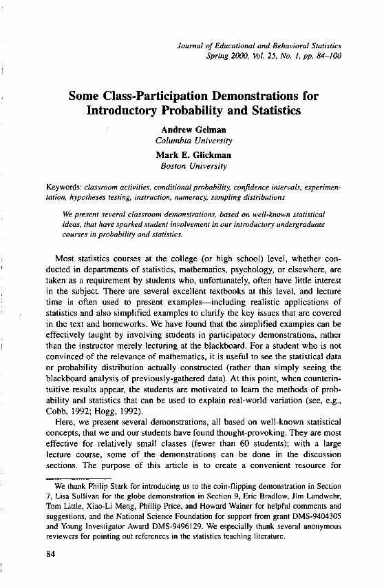
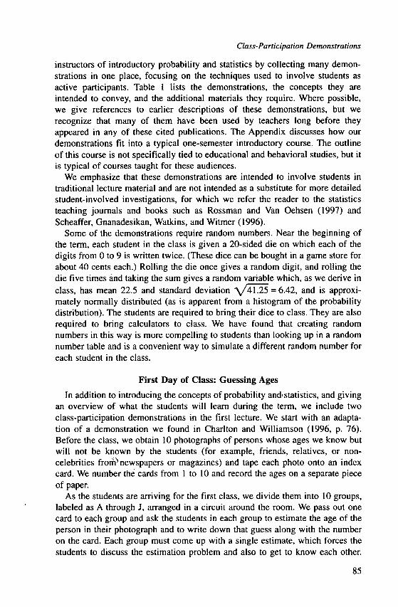
2. Give your best estimate of the percentage of countries in the United Nations that are in Africa.

A number between 0 and 100 is hand-written on the . In fact, the number is not chosen at random between 0 and 100; rather, "10" is written on half the forms and "65" is written on the other half, and the forms are shuffled before handing them out to the students.

After the students have answered the questions and returned the forms, we explain to the students that only two values of X were actually assigned I and that we were interested in finding the relation between X and the students' responses on the second question. We then ask the students what kind of data collection was happening: survey, experiment, or observational study. In statistical termi- nology, the units are the students, the treatments are the hand-written values of X (10 or 65), and the outcome of interest is the response to the second question. This is adapted from an experiment described in Kahneman and Tversky (1974), who report that the median responses to the second question are 25 and 45, given X = l0 and 65, respectively. This is described as an example of the "anchoring heuristic," in which an estimate of an unknown quantity is influ- enced by a previously-supplied starting point. In this example, the value of X should not effect the outcome (after all, the students were told that X was randomly generated), yet it does! This is a good point to discuss the principles of randomization and blindness in experimentation, now that the students have had it done to them. Incidentally, the actual value of the unknown quantity is irrelevant for this example--all that we are studying is the differences in responses between the two groups of students.

In performing this example in our classes, we have replicated the anchoring effect, although its magnitude has not been so dramatic as found by Kahneman and Tversky; for example, histograms of responses for a class of 43 students are given in Figure I. When the data have been collected, the two groups can

88

0

rn

¢D

0


r- - I 0 20 40 60 . 80 100

treatment=-65

N

0

aO

,¢

0

0 20 40 60 80 1 O0

treatment=lO

FIGURE 1. Responses of students in a small introductory probability and statistics class to the question, "Give your best estimate of the percentage of countries in the United Nations that are in Africa." The students were previously asked to compare this percentage with a specified value X; histogram (a) displays responses for students given X = 65, and histogram (b) displays responses for students given X = 10. The students were told that the value of X was chosen at random, and yet it has an effect (on average) on their responses. Similar results were obtained when the experiment was repeated in other classes. Adapted from an experiment described in Kahneman and Tversky (1974).

immediately be compared graphically using histograms; typically, as in Figure 1, the histograms overlap considerably but clearly differ. The dataset can be used throughout the course to illustrate various points of statistics, including the mean and median in skewed distributions, methods of testing the statistical significance of observed differences between groups, and the distinction between practical and statistical significance. With classes of about 50 students, we have

89

Gelman and Glickman

found the anchoring effect in this experiment to be on the border of statistical significance as measured by a t test.

Other examples in which an experiment is embedded in a survey include studies of question wording, question ordering, and other causes of survey response bias; see Scheaffer et al. (1996, pp. 284-288), for a related classroom demonstration. In addition, the experiment given here could be complexified by randomly ordering the options "higher" and "lower" in the first question of the survey, thus giving two factors and four possible experimental conditions.

How Large is Your Family?

The following demonstration helps teach principles of survey sampling. Each student is asked to tell how many children are in his or her family (that is, the number of brothers and sisters in your family, including yourself). We write the results on the blackboard as a frequency table and a histogram, and then compute the mean, which is typically around 3. We tell the students that the average number of children in families that were having children 20 years ago (about the age of the students in the class) was about 2.0. Why is the number for this class so high? Students give various suggestions such as, perhaps larger families are more likely to send children to college. After some discussion, a student notes that if the family had zero children, they certainly did not send any to college. The 2.0 figure is the average number of children when sampling by family; 3.0 is the average number of children when sampling by child. When sampling by child, a family with n children is n times more likely to be sampled than a family with 1 child. This illustrates the general point that it is not enough to say you sampled at random; you must also know the sampling units. It can also be considered as an example of sampling bias. At this point, we can get the students further involved by asking the question, how can data be gathered to estimate the average number of children per household? In discussing the problem, students can consider the relative difficulties of correcting the data on students for sampling bias, compared to the direct approach of sampling families. The former approach is tricky because it still requires some estimate of the proportion of families with zero children. The students also have to realize that, for either approach, a careful definition of "family" is required. This example is discussed in more detail by Madsen (1981).

Related issued arise in telephone sampling, when you call a telephone number at random and then pick a person at random in that household to interview: Is a person with many phone lines more or less likely to be sampled than a person with one line? Is a person with many roommates more or less likely to be sampled than a person living alone (see Gelman & Little, 1998)? Another area in which size-biased sampling can occur is clinical psychiatry; see Cohen and Cohen (1984) for an interesting and accessible discussion.

90


Lie Detectors and Conditional Probability

In teaching conditional probability, we embed a well-known example in a dramatic setting to get students directly involved with the problem. The scenario is as follows. Through accounting procedures, it is known that about 10% of the employees of a store are stealing. We pick two students to play the role of "managers," and the other students in the class are the "employees." The managers would like to fire the thieves, but their only tool in distinguishing them from the honest employees is a lie detector test that is 80% accurate: if an employee is a thief, he or she will fail the test with probability 0.8, and if an employee is not a thief, he or she will pass the test with probability 0.8.

To simulate these conditions, each employee rolls a die on which are written the digits from 0 to 9. If the die roll is in the range 1-9, the employee is honest; if it comes up "0," he or she is a thief. In either case, however, the employee does not reveal this outcome to anyone else. Instead, he or she rolls the die again to determine the outcome of the lie detector test. If the die roll is in the range 2-9, the lie detector gives the correct answer ("pass" for an honest employee, "fail" for a thief); if it comes up "0" or "1," the lie detector gives the wrong answer and records "fail" for an honest employee and "pass" for a thief. The employees who have failed the lie detector test are asked to raise their hands. For example, in a class of 50 students, one would expect about 50 x 0.26 = 13 students to raise their hands.

The managers are then asked, "How many of those employees do you think are thieves?" A typical response is that about 80% of those who failed the lie detector test are thieves. The students who have raised their hands are now asked to tell their true status--honest or thief--and, in fact, it generally turns out that most are honest! The mistake made by the managers is the well-known fallacy of reversing the conditional probability (assuming Pr[AIB] = Pr[BIA]), which is also explained in terms of neglecting the base rate (Tversky & Kahneman, 1982).

We then explain the correct reasoning by drawing a probability tree that has branches indicating "honest" or "thief," each of which has branches indicating "pass" or "fail." The total probability of "fail" is (0.1)(0.8) + (0.9)(0.2) = 0.26, and the conditional probability of "thief," given "fail," is Pr("thief"l"fair ' ) = Pr("thief" and "fail")/Pr("fair ') = 0.08/0.26 = 0.31: if you fail the test, there is only a 31% probability that you are a thief. We also explain by expressing the possible outcomes of the die rolls as a 10 x 10 table with the row and columns indicating the results of the first and second die rolls, respectively. The top row of the table corresponds to the thieves, and the left two columns correspond to the lie detector giving the wrong answer. It is clear that there are 18 ways to be honest and fail the lie detector test, but only 8 ways to be a thief and fail.

Another example of this phenomenon of a high false-positive rate, in medical testing, has been recommended in statistics teaching (see Moore, 1990, pp. 123-124); whatever the context, we recommend that the student-participation version precede formal presentation of tree diagrams and conditional probability.

91

Gelman and Glickman

Real Versus Fake Coin Flips

Students often have difficulty thinking about summary statistics as random variables with probability distributions. This demonstration, which also alerts students to misconceptions about randomness, nicely motivates the concept of the sampling distributiori.

As discussed by Kahneman and Tversky (1974), people generally believe that a sequence of coin flips should have a haphazard pattern, including frequent (but not regular) alternations between heads and tails. In fact, it is quite common for long runs of heads and tails to appear in sequences of random coin flips.

The demonstration, which is an adaptation of idea suggested to us by Prof. Philip Stark (see also Gnanadesikan, Scheaffer, Watkins, & Witmer, 1997, Revesz, 1978, and Schilling, 1990), proceeds as follows. We pick two students to be "judges" and one to be the "recorder" and divide the others in the class into two groups. One group is instructed to flip a coin 100 times, or flip I0 coins 10 times each, or follow some similarly defined protocol, and then to write the results, in order, on a sheet of paper, writing heads as "1" and tails as "0" (because "H" and "T" look similar and can be confused when reading them off a sheet of paper). The second group is instructed to create a sequence of 100 "0"s and " l " s that are intended to look like the result of coin fl ips--but they are to do this without flipping any coins or using any randomization device (or consulting with the other group of students)--and to write this sequence on a sheet of paper. The recorder is instructed to copy these sequences onto two blackboards. We announce that the instructor and the judges will leave the room for five minutes while the students create their sequences, and then we will return and try to guess which sequence is from actual coin flips and which was made up.

We return to the room, examine the sequences written on the two blackboards, and ask the judges to guess which sequence is real. We then identify the sequence of real coin flips; invariably the identification is correct, and the students are impressed. How did we do it? Well, even as the sequences are being written on the blackboard, the students notice a difference: the sequence of fake coin flips looks "random" in an orderly sort of way, with frequent switches between O's and l 's, whereas the sequence of real coin flips has a "streaky" look to it, with one or more long runs of successive O's or l 's. (Revesz, 1978, suggests distinguishing between real and fake sequences using a formal rule based on the longest run length, but we find that we can make the distinction more effectively based on a visual inspection of the sequences, which implicitly takes into account much more information.)

We picked out the real sequence using our experience and knowledge of coin flips. How can this reasoning be formalized? For each of the two sequences on the blackboards, we count the number of runs (sequences of O's and 1 's) and the length of the longest run. We then hand out copies of Figure 2, which shows the sampling distributions of these two statistics, as simulated from 2000 independent computer simulations of 100 coin flips. The students are instructed to

92

¢ -

2

cD O ) ¢ -

o 0 c -

e -

¢ D v - .

, ¢

O0

CO

,q¢


• . ' , ' . .

• ' " . : - . b " . ' " " ' "

. : ; . . . ' . ~.: ': .=' .: ," ..

" : ~'-".~ ; ; ~ ' ~ ";-~,. : 1 ~ / " ~ ' ~ . . ' . • ' •

• . ".~ ":,~ ? ~ t ~ t ' ~ * .',.., ~ - . . .

I I I

40 50 60

Number of switches

FIGURE 2. Length of longest run (sequence of successive heads or successive tails) versus number of runs (sequences of heads or tails) in each of 2000 independent simulations of 100 coin flips. Each dot on the graph represents a sequence of 100 coin flips; the points are jittered so they do not overlap. When plotted on this graph, the results from an actual sequence of 100 coin flips will most likely fall on a square with a large number of dots. In contrast, a sequence of heads and tails that is artificially created to look "random "' will probably have too many runs that are not long enough, and hence will fall on the lower right of this graph.

circle on the scatterplot the locations of the values for the sequences on the blackboard. All the times we have used this example in class, the sequence of real coin flips is near the center of the scatterplot, and the sequence of fake coin flips has too many runs and too short a longest run, compared to this distribution.

In addition to its "magic trick" aspect, this demonstration is appealing because it dramatically illustrates an important point for the interpretation of data: seemingly surprising patterns (long sequences of heads or tails) can occur entirely at random, with no external cause. Long runs in real coin-flip data surprise students because they expect that any part of a random sequence will itself look " random"- - tha t is, typical of the whole• This can be the starting point of a discussion of the general phenomenon that small samples can be unrepre-

93

Gelman and Glickman

sentative of a population. Familiar examples include biological data (for example, a family can have several boys or girls in a row) and sports (a basketball player can have "hot" and "cold" streaks that are consistent with random fluctuation; see Gilovich, Vallone, & Tversky, 1985).

A Coincidence?

We have found a rigged guessing game similar to those described in Eckert (1994) and Maxwell (1994) to be useful for illustrating the underlying principles of classical hypothesis testing. The general idea is to have a student guess a low-probability event and then, through a faked randomization process, find that the guess is indeed correct. The resulting surprise, followed by skepticism, of the class leads to an exploration of hypotheses testing and p-values.

Maxwell (1994) presents a demonstration based on a student's correctly guessing a series of coin flips (reminiscent of the opening scene of Stoppard, 1967). We have had success using the "Invisible Deck," a card trick that can be bought from most magic suppliers for $5-$10 and is fairly simple to perform with a little practice.

We tell the class that before leaving the office, we chose a card at random, turned it upside down, and replaced it back in the deck. We then select a student at random. It is essential that it is clear the student was selected randomly (for example by choosing the student with highest "IQ" from the previous demonstration).

The student is asked to guess the hidden card and write the guess on the blackboard. We then fan the special deck of cards showing that there is a single card that is face down while the rest of the cards are face up. We remove the card without showing its face and attach it to the blackboard with a piece of masking tape. Up to this point, the students think that we have simply removed the card that we turned face down before coming to class, when, in actuality, we have used the trick to remove the card named by the student.

Suppose the student named the Jack of Spades. We remind the class that because the student had no knowledge of the card we reversed before coming to class, the probability that the face-clown card is the Jack of Spades is 1/52. We then ask the students if they would be nonetheless surprised that the face-down card was the same color as the Jack of Spades, that is, black. After the class says no, we ask them to explain why they think it would not be surprising. Depending on the responses, we usually clarify that there is a 1/2 probability that the card would be black, assuming the student naming the Jack of Spades had no previous knowledge of the card, and that nothing else "strange" was going on. We then ask if it would be surprising that the face-down card had the same suit (Spades). Students agree that this would not be too surprising, but certainly more surprising than if it were merely black. What if the card were a Jack? This would be even more surprising. At this point, we begin to arouse suspicion that a surprising event is about to happen. We finally ask what if the card was the Jack of Spades. This would be very surprising, indeed. We remind the class that if the

94


card actually were the Jack of Spades, then they would have a choice of two conclusions. Either a very unlikely event occurred, namely one with a probability of 1/52, or our original assumption (that the process of the student naming any card and our reversing a card before coming to class were unrelated) was wrong. After a dramatic pause, we pull the taped card off the board to reveal the Jack of Spades. We then admit this demonstration was a card trick, though the students were well aware of this fact by the middle of the demonstration. The card trick is then followed by a more formal discussion of hypotheses testing.

We find the demonstration useful in motivating students to think about concepts of hypothesis testing, particularly at a foundational level. One reason is that the exercise involves a null hypothesis that appears undeniably true, and that it may be difficult to imagine how the alternative hypothesis could be correct. This emphasizes the asymmetry of the hypothesis testing framework in which we would not abandon the null hypothesis unless provided with strong evidence to the contrary. In addition, students have let us know in their comments that they find the consideration of several null hypotheses easier to grasp in the context of a classroom demonstration than in a textbook presentation.

Coverage of Confidence Intervals

At the beginning of the lecture, the students are given identical slips of paper; they are told to write their weights (in pounds) on their slips and put them in a hat that is passed around the room. When the hat is filled, it is then passed around again. Each student is told to mix up the slips in the hat, pick out four slips at random, write down the numbers, put the slips back in the hat, and pass the hat to the next student. The student should then use the four numbers to create a 90% confidence interval for the average weight of all the students in the class (with a sample size of only 4, the t interval may be only a rough approximation, but at least the students can do their computations fairly quickly). This can be all done while the lecture is proceeding. When all the students are done, they go up to the board one at a time and plot their confidence intervals on an axis (as horizontal segments, stacked vertically). Approximately 90% of these should contain the true value, which i s . . . (the teaching assistant quickly computes the mean of all the numbers in the hat), which we can draw as a vertical line on the blackboard display. The students should realize that the exact number of intervals that contain the true value should follow the binomial distribution. This demonstration dramatizes the fact that the confidence interval is itself a random quantity, subject to sampling variability. It is often recommended in statistics teaching to use stacked intervals to picture the sampling distribution of a confidence interval (see, e.g., Moore, 1990, pp. 130-131); we find the display particularly compelling when the sampling distribution is created by the students themselves.

The instructor can of course replace "weight" by the response to some more controversial question about which the students might be particularly curious.

95

Gelrnan and Glickman

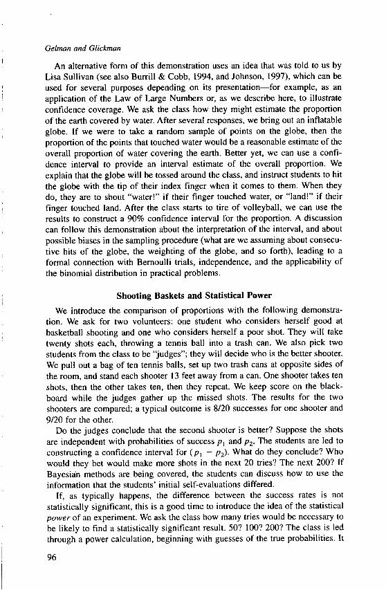
An alternative form of this demonstration uses an idea that was told to us by Lisa Sullivan (see also Burrill & Cobb, 1994, and Johnson, 1997), which can be used for several purposes depending on its presentation--for example, as an application of the Law of Large Numbers or, as we describe here, to illustrate confidence coverage. We ask the class how they might estimate the proportion of the earth covered by water. After several responses, we bring out an inflatable globe. If we were to take a random sample of points on the globe, then the proportion of the points that touched water would be a reasonable estimate of the overall proportion of water covering the earth. Better yet, we can use a confidence interval to provide an interval estimate of the overall proportion. We explain that the globe will be tossed around the class, and instruct students to hit the globe with the tip of their index finger when it comes to them. When they do, they are to shout "water!" if their finger touched water, or "land!" if their finger touched land. After the class starts to tire of volleyball, we can use the results to construct a 90% confidence interval for the proportion. A discussion can follow this demonstration about the interpretation of the interval, and about possible biases in the sampling procedure (what are we assuming about consecu- tive hits of the globe, the weighting of the globe, and so forth), leading to a formal connection with Bernoulli trials, independence, and the applicability of the binomial distribution in practical problems.

Shooting Baskets and Statistical Power

We introduce the comparison of proportions with the following demonstration. We ask for two volunteers: one student who considers herself good at basketball shooting and one who considers herself a poor shot. They will take twenty shots each, throwing a tennis ball into a trash can. We also pick two students from the class to be "judges"; they will decide who is the better shooter. We pull out a bag of ten tennis balls, set up two trash cans at opposite sides of the room, and stand each shooter 13 feet away from a can. One shooter takes ten shots, then the other takes ten, then they repeat. We keep score on the blackboard while the judges gather up the missed shots. The results for the two shooters are compared; a typical outcome is 8/20 successes for one shooter and 9/20 for the other.

Do the judges conclude that the second shooter is better? Suppose the shots are independent with probabilities of success p~ and P2. The students are led to constructing a confidence interval for (p~ - P2). What do they conclude? Who would they bet would make more shots in the next 20 tries? The next 200? If Bayesia'n methods are being covered, the students can discuss how to use the information that the students' initial self-evaluations differed.

If, as typically happens, the difference between the success rates is not statistically significant, this is a good time to introduce the idea of the statistical power of an experiment. We ask the class how many tries would be necessary to be likely to find a statistically significant result. 50? 100? 200? The class is led through a power calculation, beginning With guesses of the true probabilities. It

96


becomes clear that, even if the true difference is quite large, 20 is most likely too small a sample to distinguish between the abilities of the two shooters 2. This has obvious consequences for experiments in other contexts (such as medical treatments) as well as real-life conclusions that we draw from small samples. Conversely, when discussing the possible results from very large samples, the students can discover the distinction between statistical and practical significance: with a huge sample size, even tiny differences can become statistically significant.

Multiple Comparisons In the general population, IQ is normally distributed with a mean of 100 and a

standard deviation of 15. We tell the students that we will determine their IQ's. But instead of giving each student a test--that would take a lot of t ime--we ' l l have each student roll dice to simulate a random draw from the distribution. They know how to use five die rolls to simulate a draw from the normal distribution with mean 22.5 and standard deviation 6.42 (see introduction); what is the transformation required to get a mean of 100 and standard deviation of 15? After some discussions, the students recognize that subtracting 22.5, multiplying by 15/6.42, and adding 100 will do the trick. The students roll the dice and compute their IQ's. It might not be the right number for each student, but the distribution is right. Now we do some comparisons. If we were to compare the average IQ of men versus women in this group, would we find a difference? Yes--the difference would almost certainly not be exactly zero. Would it be statistically significant at the 5% level? After some discussion, the students realize that if the experiment were performed many times, with the same number of students, only 5% of the samples would have differences extreme enough to be "statistically significant." What about comparing freshman versus upperclass- men? Front row versus back row? Same answer. We now ask the students with IQ's above 115 to hold up two hands, those between 85 and 1 |5 to hold up one hand, and those below 85 to hold up no hands. Given this information, we construct a division of the class that has almost all the high-IQ students on one side and almost all the Iow-IQ students on the other. It is important that the divisions of the class be based on some external criteria such as position in class, whether students wear glasses, hair color, etc. (for example, comparing men in the front row to women in the back two rows). We get the IQ's for the two groups and compare and, sure enough, the difference is statistically significant! We can construct an amusing story to explain the difference (for example, the smarter women sit in the back rows because they do not need to follow the lectures carefully, etc.). But of course it is not real; the IQ's were created by rolling dice. We discuss the well-known implications of "data dredging" for scientific studies. (For example, consider a drug company that is testing 1000 new treatments. Even if they all have no effect, 50 of them will appear to be statistically significant at the 5% level. This is a motivation for formal multiple- comparisons methods such as the Bonferroni procedure.)

97

Gelman and Glickman

Conclusions

We have found student-participation demonstrations to be effective in drama- tizing concepts that students often find difficult (for example, numeracy, conditional probability, the difference between an experiment and a survey, statistical and practical significance, the sampling distribution of confidence intervals). Students are made aware that they and others are subject to cognitive illusions (in the lie detector, anchoring, and coin-flipping examples); for more on this, see, e.g., Kahneman et al. (1982) and Goldstein and Hogarth (1997). In addition, the experiments that involve data-gathering illustrate general concerns of bias and variance (in the age-guessing example) and also involve important practical issues such as time trends (shooting baskets), displaying data (experiment on anchoring, guessing exam scores), experimental protocol (age-guessing, the "United Nations" survey/experiment), and the relation between models and data (family size, sampling). One reason that we believe these demonstrations are important is that the role-playing settings emphasize that statistics is, in reality, a participatory process with many actors (typically, different people design a study, collect data, are experimental subjects, analyze data, interpret results, etc.). Finally, the demonstrations get all the students involved and help to create an environment where students feel free to participate and ask questions in class.

Appendix

The Demonstrations in the Context o f a One-Semester Statistics Course

The demonstrations in this paper are presented as separate modules so that the reader can easily use any or all of them. In any given course, however, we want to avoid the impression of statistics as a set of unrelated methods and examples. This appendix illustrates how we intergrate our demonstrations and other teaching material into a standard non-calculus-based thirteen-week one-semester introductory course based on a textbook such as Moore and McCabe (1998). For each week, we outline the course material and the relevant demonstrations.

1. Introduction; data in one dimension (guessing ages; estimating a big number)

2. Data in two dimensions: scatterplots and least-squares 3. Data in two dimensions: log transformations (discussion of estimating a big

number) 4. Data in two and three dimensions: correlation and categorical data 5. Causal inference and experiments (an experiment that looks like a survey) 6. Sampling; statistical inference; bias and variance (how large is your family;

also, discussion of the data from guessing ages) 7. Probability trees and conditional probability (lie detectors) 8. Random variables in one and two dimensions 9. Sums of random variables; binomial distribution 10. Confidence intervals and significance tests (real versus fake coin flips; a

coincidence)

98


11. The t distribution; applications to surveys and experiments (coverage of confidence intervals)

12. Inference for proportions and simple linear regression (shooting baskets) 13. Statistical communication: how to lie and tell the truth with statistics

(multiple comparisons)

During the weeks in which none of the demonstrations in this article is sched- uled, we set aside some class time for students to work together on problems in small groups (see, e.g., Magel, 1998). Whenever possible, we motivate and introduce the topics through examples that involve the students, and then we develop the relevant statistical methods. In addition, in later lectures, we often refer back to the demonstrations as well as to other data-collection exercises from students' exams (see Gelman, 1997).

Notes

~If the experiment were actually performed with random numbers, the analysis would be somewhat more complicated, because there would then be a continuous range of possible treatments.

2For example, if the true probabilities of success of the two students are 0.4 and 0.5, and each student shoots 100 baskets, then the standard deviation of the observed difference in proportions is ~¢/(0.4)(0.6)/100+(0.5)(0.5)/100 = 0.071, so that the true difference is still less than two standard errors away from zero.

References

Burrill, G., & Cobb, G. (1994). Everyone's favorite subject: what's new. Stats. Charlton, J., & Williamson, R. (1996). Practical exercises in applied statistics. Oxford:

Oxford University Press. Cobb, G. (1992). Teaching statistics. In L. A. Steen (Ed.), Heeding the call for change:

Suggestions for curricular action (pp. 3-34). Mathematical Association of America. Cohen, P., & Cohen, J. (1984). The clinician's illusion. Archives of General Psychiatry,

41, 1178-1182. Eckert, S. (1994). Teaching hypothesis testing with playing cards: A demonstration.

Journal of Statistics Education, 2 ( 1 ). Gelman, A. (1997). Using exams for teaching concepts in probability and statistics.

Journal of Educational and Behavioral Statistics, 22, 237-243. Gelman, A., & Little, T. C. (1998). Improving upon probability weighting for household

size. Public Opinion Quarterly, to appear. George, P. A., & Hole, G. J. (1995). Factors influencing the accuracy of age estimates of

unfamiliar faces. Perception, 24, 1059-1073. Gilovich, T., Vallone, R., & Tversky, A. (1985). The hot hand in basketball: on the

misperception of random sequences. Cognitive Psychology, 17, 295-314. Gnanadesikan, M., Scheaffer, R. L., Watkins, A. E., & Witmer, J. A. (1997). An activity-

based statistics course. Journal of Statistics Education, 5 (2). Goldstein, W. M., & Hogarth, R. M. (1997). Research on judgment and decision making.

Cambridge: Cambridge University Press.

99

Gelman and Glickman

Hogg, R.V. (1992). Report of workshop on statistical education. In L. A. Steen (Ed.), Heeding the call for change: Suggestions for curricular action, (pp. 34-43). Math- ematical Association of America.

Johnson, R. (1997). Earth's surface water percentage? Teaching Statistics, 19, 66-68. Kahneman, D., SIovic, P., & Tversky, A. (1982). Judgment Under Uncertainty: Heuris-

tics and Biases. Cambridge: Cambridge University Press. Kahneman, D., & Tversky, A. (1974). Judgment under uncertainty: heuristics and biases.

Science, 185, 1124-1131. Reprinted in Kahneman, Slovic, & Tversky (1982). Madsen, R. W. (1981). Making students aware of bias. Teaching Statistics, 3, 2-5. Magel, R. C. (1998). Using cooperative learning in a large introductory statistics class.

Journal of Statistics Education, 6 (3). Maxwell, N. E (1994). A coin-flipping exercise to introduce the P-value. Journal of

Statistics Education, 2 (!). Moore, D. S. (1990). Uncertainty. In L. A. Steen (Ed.), On the shoulders of giants: New

approaches to numeracy, (pp. 95-137). Washington, D.C.: National Academy Press. Moore, D. A., & McCabe, G. P. (1998). Introduction to the practice of statistics, third

edition. New York: Freeman. Paulos, J. A. (1988). Innumeracy: Mathematical illiteracy and its consequences. New

York: Hill and Wang. Revesz, P. (1978). Strong theorems on coin tossing. Proceedings of the International

Congress of Mathematicians, 749-754. Rossman, A., & Von Oehsen, J. B. (1997). Workshop statistics: Discovery with data and

the graphing calculator. New York: Springer-Verlag. Schilling, M. E (1990). The longest run of heads. The College Mathematics Journal, 21,

196-207. Scheaffer, R.L., Gnanadesikan, M., Watkins, A., & Witmer, J. (1996). Activity-based

statistics: Instructor resources. New York: Springer-Verlag. Stoppard, T. (1967). Rosenkrantz and Guildenstern are dead. London: Faber and Faber. Tversky, A., & Kahneman, D. (1982). Evidential impact of base rates. In D. Kahneman,

P. Slovic, and A. Tversky (Eds.), Judgment under uncertainty: Heuristics and biases, (pp. 153-160). Cambridge University Press.

Authors

ANDREW GELMAN is Associate Professor of Statistics and Director of the Quantitative Methods in Social Science Program at Columbia University, New York, NY 10027; [email protected]. His research interests include public health and policy, statistical graphics, and Bayesian data analysis.

MARK E. GLICKMAN is Assistant Professor of Mathematics and Statistics at Boston University, Boston, MA 02215; [email protected]. His research interests include Bayesian statistics, health services research, and paired comparison models.

¢

I00

some class-participation demonstrations for introductory ...€¦ · courses in probability and...

Documents