bayesian statistics - courses - university of california, santa cruz

Bayesian Statistics B 455

Bayesian StatisticsDAVID DRAPERDepartment of Applied Mathematics and Statistics,Baskin School of Engineering, University of California,Santa Cruz, USA

456 B Bayesian Statistics

Article Outline

GlossaryDefinition of the Subject and IntroductionThe Bayesian Statistical ParadigmThree ExamplesComparison with the Frequentist Statistical ParadigmFuture DirectionsBibliography

Glossary

Bayes’ theorem; prior, likelihood and posteriordistributions Given (a) � , something of interest which is

unknown to the person making an uncertainty as-sessment, conveniently referred to as You, (b) y, aninformation source which is relevant to decreasingYour uncertainty about � , (c) a desire to learn about �from y in a way that is both internally and externallylogically consistent, and (d) B, Your background as-sumptions and judgments about how the world works,as these assumptions and judgments relate to learningabout � from y, it can be shown that You are com-pelled in this situation to reason within the standardrules of probability as the basis of Your inferencesabout � , predictions of future data y�, and decisionsin the face of uncertainty (see below for contrastsbetween inference, prediction and decision-making),and to quantify Your uncertainty about any unknownquantities through conditional probability distribu-tions. When inferences about � are the goal, Bayes’Theorem provides a means of combining all relevantinformation internal and external to y:

p(� jy;B) D c p(� jB) l(� jy;B) : (1)

Here, for example in the case in which � is a real-val-ued vector of length k, (a) p(� jB) is Your prior dis-tribution about � given B (in the form of a proba-bility density function), which quantifies all relevantinformation available to You about � external to y,(b) c is a positive normalizing constant, chosen tomake the density on the left side of the equation in-tegrate to 1, (c) l(� jy;B) is Your likelihood distribu-tion for � given y and B, which is defined to be a den-sity-normalized multiple of Your sampling distribu-tion p(�j�;B) for future data values y� given � andB, but re-interpreted as a function of � for fixed y,and (d) p(� jy;B) is Your posterior distribution about �given y and B, which summarizes Your current to-tal information about � and solves the basic inferenceproblem.

Bayesian parametric and non-parametric modeling (1)Following de Finetti [23], a Bayesian statistical modelis a joint predictive distribution p(y1; : : : ; yn) for ob-servable quantities yi that have not yet been observed,and about which You are therefore uncertain. Whenthe yi are real-valued, often You will not regard themas probabilistically independent (informally, the yi areindependent if information about any of them doesnot help You to predict the others); but it may be pos-sible to identify a parameter vector � D (�1; : : : ; �k)such that You would judge the yi conditionally inde-pendent given � , and would therefore be willing tomodel them via the relation

p(y1; : : : ; yn j�) DnY

iD1

p(yi j�) : (2)

When combined with a prior distribution p(�) on �that is appropriate to the context, this is Bayesianparametric modeling, in which p(yi j�) will often havea standard distributional form (such as binomial, Pois-son or Gaussian). (2) When a (finite) parameter vec-tor that induces conditional independence cannot befound, if You judge your uncertainty about the real-valued yi exchangeable (see below), then a representa-tion theorem of de Finetti [21] states informally that allinternally logically consistent predictive distributionsp(y1; : : : ; yn) can be expressed in a way that is equiv-alent to the hierarchical model (see below)

(FjB) � p(FjB)(yi jF;B) IID

� F ;(3)

where (a) F is the cumulative distribution function(CDF) of the underlying process (y1; y2; : : : ) fromwhich You are willing to regard p(y1; : : : ; yn) as (ineffect) like a random sample and (b) p(FjB) is Yourprior distribution on the space F of all CDFs on thereal line. This (placing probability distributions on in-finite-dimensional spaces such as F) is Bayesian non-parametric modeling, in which priors involvingDirich-let processes and/or Pólya trees (see Sect. “Inference:Parametric and Non-Parametric Modeling of CountData”) are often used.

Exchangeability A sequence y D (y1; : : : ; yn) of randomvariables (for n � 1) is (finitely) exchangeable if thejoint probability distribution p(y1; : : : ; yn) of the el-ements of y is invariant under permutation of theindices (1; : : : ; n), and a countably infinite sequence(y1; y2; : : : ) is (infinitely) exchangeable if every finitesubsequence is finitely exchangeable.


Hierarchical modeling Often Your uncertainty aboutsomething unknown to You can be seen to havea nested or hierarchical character. One class of ex-amples arises in cluster sampling in fields such aseducation and medicine, in which students (level 1)are nested within classrooms (level 2) and patients(level 1) within hospitals (level 2); cluster sampling in-volves random samples (and therefore uncertainty) attwo or more levels in such a data hierarchy (exam-ples of this type of hierarchical modeling are givenin Sect. “Strengths and Weaknesses of the Two Ap-proaches”). Another, quite different, class of exam-ples of Bayesian hierarchical modeling is exemplifiedby equation (3) above, in which is was helpful to de-compose Your overall predictive uncertainty about(y1; : : : ; yn) into (a) uncertainty about F and then(b) uncertainty about the yi given F (examples of thistype of hierarchical modeling appear in Sect. “Infer-ence and Prediction: Binary Outcomes with No Co-variates” and “Inference: Parametric and Non-Para-metric Modeling of Count Data”).

Inference, prediction and decision-making; samplesand populations Given a data source y, inference involves

drawing probabilistic conclusions about the underly-ing process that gave rise to y, prediction involvessummarizing uncertainty about future observable datavalues y�, and decision-making involves looking foroptimal behavioral choices in the face of uncertainty(about either the underlying process, or the future,or both). In some cases inference takes the form ofreasoning backwards from a sample of data values toa population: a (larger) universe of possible data val-ues from which You judge that the sample has beendrawn in a manner that is representative (i. e., so thatthe sampled and unsampled values in the populationare (likely to be) similar in relevant ways).

Mixture modeling Given y, unknown to You, and B,Your background assumptions and judgments rele-vant to y, You have a choice: You can either model(Your uncertainty about) y directly, through the prob-ability distribution p(yjB), or (if that is not feasible)You can identify a quantity x upon which You judge yto depend and model y hierarchically, in two stages:first by modeling x, through the probability distribu-tion p(xjB), and then by modeling y given x, throughthe probability distribution p(yjx;B):

p(yjB) DZ

Xp(yjx;B) p(xjB) dx ; (4)

whereX is the space of possible values of x over whichYour uncertainty is expressed. This is mixture model-

ing, a special case of hierarchical modeling (see above).In hierarchical notation (4) can be re-expressed as

y D�

x(yjx)

�: (5)

Examples of mixture modeling in this article include(a) equation (3) above, with F playing the role of x;(b) the basic equation governing Bayesian prediction,discussed in Sect. “The Bayesian Statistical Paradigm”;(c) Bayesian model averaging (Sect. “The BayesianStatistical Paradigm”); (d) de Finetti’s representationtheorem for binary outcomes (Sect. “Inference andPrediction: Binary Outcomes with No Covariates”);(e) random-effects parametric and non-parametricmodeling of count data (Sect. “Inference: Parametricand Non-Parametric Modeling of Count Data”); and(f) integrated likelihoods in Bayes factors (Sect. “Deci-sion-Making: Variable Selection in Generalized LinearModels; Bayesian Model Selection”).

Probability – frequentist and Bayesian In the frequen-tist probability paradigm, attention is restricted to phe-nomena that are inherently repeatable under (essen-tially) identical conditions; then, for an event A of in-terest, Pf (A) is the limiting relative frequency withwhich A occurs in the (hypothetical) repetitions, asthe number of repetitions n!1. By contrast, YourBayesian probability PB(AjB) is the numerical weightof evidence, given Your background information Brelevant to A, in favor of a true-false proposition Awhose truth status is uncertain to You, obeying a se-ries of reasonable axioms to ensure that Your Bayesianprobabilities are internally logically consistent.

Utility To ensure internal logical consistency, optimal de-cision-making proceeds by (a) specifying a utility func-tion U(a; �0) quantifying the numerical value associ-ated with taking action a if the unknown is really �0and (b) maximizing expected utility, where the expec-tation is taken over uncertainty in � as quantified bythe posterior distribution p(� jy;B).

Definition of the Subject and Introduction

Statistics may be defined as the study of uncertainty:how to measure it, and how to make choices in theface of it. Uncertainty is quantified via probability, ofwhich there are two leading paradigms, frequentist (dis-cussed in Sect. “Comparison with the Frequentist Statisti-cal Paradigm”) and Bayesian. In the Bayesian approach toprobability the primitive constructs are true-false proposi-tions A whose truth status is uncertain, and the probabil-ity of A is the numerical weight of evidence in favor of A,


constrained to obey a set of axioms to ensure that Bayesianprobabilities are coherent (internally logically consistent).

The discipline of statistics may be divided broadly intofour activities: description (graphical and numerical sum-maries of a data set y, without attempting to reason out-ward from it; this activity is almost entirely non-proba-bilistic and will not be discussed further here), inference(drawing probabilistic conclusions about the underlyingprocess that gave rise to y), prediction (summarizing un-certainty about future observable data values y�), and de-cision-making (looking for optimal behavioral choices inthe face of uncertainty). Bayesian statistics is an approachto inference, prediction and decision-making that is basedon the Bayesian probability paradigm, in which uncer-tainty about an unknown � (this is the inference prob-lem) is quantified by means of a conditional probabilitydistribution p(� jy;B); here y is all available relevant dataandB summarizes the background assumptions and judg-ments of the person making the uncertainty assessment.Prediction of a future y� is similarly based on the condi-tional probability distribution p(y�jy;B), and optimal de-cision-making proceeds by (a) specifying a utility functionU(a; �0) quantifying the numerical reward associated withtaking action a if the unknown is really �0 and (b) maxi-mizing expected utility, where the expectation is taken overuncertainty in � as quantified by p(� jy;B).

The Bayesian Statistical Paradigm

Statistics is the branch of mathematical and scientificinquiry devoted to the study of uncertainty: its conse-quences, and how to behave sensibly in its presence. Thesubject draws heavily on probability, a discipline whichpredates it by about 100 years: basic probability theory canbe traced [48] to work of Pascal, Fermat and Huygens inthe 1650s, and the beginnings of statistics [34,109] are ev-ident in work of Bayes published in the 1760s.

The Bayesian statistical paradigm consists of three ba-sic ingredients:

� � , something of interest which is unknown (or onlypartially known) to the person making the uncertaintyassessment, conveniently referred to, in a conventionproposed by Good (1950), as You. Often � is a param-eter vector of real numbers (of finite length k, say) ora matrix, but it can literally be almost anything: for ex-ample, a function (three leading examples are a cumu-lative distribution function (CDF), a density, or a re-gression surface), a phylogenetic tree, an image of a re-gion on the surface of Mars at a particular moment intime, : : :

� y, an information source which is relevant to decreasingYour uncertainty about � . Often y is a vector of realnumbers (of finite length n, say), but it can also literallybe almost anything: for instance, a time series, a movie,the text in a book, : : :

� A desire to learn about � from y in a way that is both co-herent (internally consistent: in other words, free of in-ternal logical contradictions; Bernardo and Smith [11]give a precise definition of coherence) and well-cali-brated (externally consistent: for example, capable ofmaking accurate predictions of future data y�).

It turns out [23,53] that You are compelled in this sit-uation to reason within the standard rules of probabil-ity (see below) as the basis of Your inferences about � ,predictions of future data y�, and decisions in the faceof uncertainty, and to quantify Your uncertainty aboutany unknown quantities through conditional probabilitydistributions, as in the following three basic equations ofBayesian statistics:

p(� jy;B) D c p(� jB) l(� jy;B)

p(y�jy;B) DZ

�

p(y�j�;B) p(� jy;B) d�

a� D argmaxa2A

E(� jy;B)�U(a; �)

�:

(6)

(The basic rules of probability [71] are: for any true-false propositions A and B and any background as-sumptions and judgmentsB, (convexity) 0 � P(AjB) � 1,with equality at 1 iff A is known to be true under B;(multiplication) P(A and BjB) D P(AjB) P(BjA;B) DP(BjB) P(AjB;B); and (addition) P(A or BjB) D P(AjB)C P(BjB)� P(A and BjB).)

The meaning of the equations in (6) is as follows.

� B stands for Your background (often not fully stated)assumptions and judgments about how the worldworks, as these assumptions and judgments relate tolearning about � from y. B is often omitted from thebasic equations (sometimes with unfortunate conse-quences), yielding the simpler-looking forms

p(� jy) D c p(�) l(� jy)

p(y�jy) DZ

�

p(y�j�) p(� jy) d�

a� D argmaxa2A

E(� jy)�U(a; �)

�:

(7)

� p(� jB) is Your prior information about � given B, inthe form of a probability density function (PDF) orprobability mass function (PMF) if � lives continuouslyor discretely on Rk (this is generically referred to as


Your prior distribution), and p(� jy;B) is Your poste-rior distribution about � given y and B, which summa-rizes Your current total information about � and solvesthe basic inference problem. These are actually not verygood names for p(� jB) and p(� jy;B), because (for ex-ample) p(� jB) really stands for all (relevant) informa-tion about � (given B) external to y, whether that in-formation was obtained before (or after) y arrives, but(a) they do emphasize the sequential nature of learn-ing and (b) through long usage it would be difficult formore accurate names to be adopted.

� c (here and throughout) is a generic positive normal-izing constant, inserted into the first equation in (6) tomake the left-hand side integrate (or sum) to 1 (as anycoherent distribution must).

� p(y�j�;B) is Your sampling distribution for future datavalues y� given � and B (and presumably You woulduse the same sampling distribution p(yj�;B) for (past)data values y, mentally turning the clock back to a pointbefore the data arrives and thinking about what valuesof y You might see). This assumes that You are willingto regard Your data as like random draws from a pop-ulation of possible data values (an heroic assumptionin some cases, for instance with observational ratherthan randomized data; this same assumption arises inthe frequentist statistical paradigm, discussed belowin Sect. “Comparison with the Frequentist StatisticalParadigm”).

� l(� jy;B) is Your likelihood function for � given y andB, which is defined to be any positive constant multi-ple of the sampling distribution p(yj�;B) but re-inter-preted as a function of � for fixed y:

l(� jy;B)D c p(yj�;B) : (8)

The likelihood function is also central to one of themain approaches to frequentist statistical inference, de-veloped by Fisher [37]; the two approaches are con-trasted in Sect.“Comparison with the Frequentist Sta-tistical Paradigm”.All of the symbols in the first equation in (6) have nowbeen defined, and this equation can be recognized asBayes’ Theorem, named after Bayes [5] because a specialcase of it appears prominently in work of his that waspublished posthumously. It describes how to pass co-herently from information about � external to y (quan-tified in the prior distribution p(� jB)) to informationboth internal and external to y (quantified in the poste-rior distribution p(� jy;B)), via the likelihood functionl(� jy;B): You multiply the prior and likelihood point-wise in � and normalize so that the posterior distribu-tion p(� jy;B) integrates (or sums) to 1.

� According to the second equation in (6), p(y�jy;B),Your (posterior) predictive distribution for futuredata y� given (past) data y and B, which solves thebasic prediction problem, must be a weighted aver-age of Your sampling distribution p(y�j�;B) weightedby Your current best information p(� jy;B) about �given y andB; in this integral is the space of possiblevalues of � over which Your uncertainty is expressed.(The second equation in (6) contains a simplifying as-sumption that should be mentioned: in full generalitythe first term p(y�j�;B) inside the integral would bep(y�jy; �;B), but it is almost always the case that theinformation in y is redundant in the presence of com-plete knowledge of � , in which case p(y�jy; �;B) Dp(y�j�;B); this state of affairs could be described bysaying that the past and future are conditionally inde-pendent given the truth. A simple example of this phe-nomenon is provided by coin-tossing: if You are watch-ing a Bernoulli(�) process unfold (see Sect. “Inferenceand Prediction: Binary Outcomes with No Covariates”)whose success probability � is unknown to You, the in-formation that 8 of the first 10 tosses have been heads isdefinitely useful to You in predicting the 11th toss, butif instead You somehow knew that � was 0.7, the out-come of the first 10 tosses would be irrelevant to You inpredicting any future tosses.)

� Finally, in the context of making a choice in the face ofuncertainty,A is Your set of possible actions, U(a; �0)is the numerical value (utility) You attach to taking ac-tion a if the unknown is really �0 (specified, withoutloss of generality, so that large utility values are pre-ferred by You), and the third equation in (6) says thatto make the choice coherently You should find the ac-tion a� thatmaximizes expected utility (MEU); here theexpectation

E(� jy;B)�U(a; �)

�D

Z

�

U(a; �) p(� jy;B) d� (9)

is taken over uncertainty in � as quantified by the pos-terior distribution p(� jy;B).

This summarizes the entire Bayesian statistical paradigm,which is driven by the three equations in (6). Examplesof its use include clinical trial design [56] and analy-sis [105]; spatio-temporal modeling, with environmentalapplications [101]; forecasting and dynamic linear mod-els [115]; non-parametric estimation of receiver operat-ing characteristic curves, with applications in medicineand agriculture [49]; finite selection models, with healthpolicy applications [79]; Bayesian CART model search,with applications in breast cancer research [16]; construc-


tion of radiocarbon calibration curves, with archaeologicalapplications [15]; factor regression models, with applica-tions to gene expression data [114]; mixture modeling forhigh-density genotyping arrays, with bioinformatic appli-cations [100]; the EM algorithm for Bayesian fitting of la-tent process models [76]; state-spacemodeling, with appli-cations in particle-filtering [92]; causal inference [42,99];hierarchical modeling of DNA sequences, with genetic andmedical applications [77]; hierarchical Poisson regressionmodeling, with applications in health care evaluation [17];multiscale modeling, with engineering and financial ap-plications [33]; expected posterior prior distributions formodel selection [91]; nested Dirichlet processes, with ap-plications in the health sciences [96]; Bayesian methodsin the study of sustainable fisheries [74,82]; hierarchicalnon-parametric meta-analysis, with medical and educa-tional applications [81]; and structural equation model-ing of multilevel data, with applications to health pol-icy [19].

Challenges to the paradigm include the following:

� Q: How do You specify the sampling distribution/likelihood function that quantifies the informationabout the unknown � internal to Your data set y?A: (1) The solution to this problem, which is commonto all approaches to statistical inference, involves imag-ining future data y� from the same process that hasyielded or will yield Your data set y; often the variabil-ity You expect in future data values can be quantified(at least approximately) through a standard parametricfamily of distributions (such as the Bernoulli/binomialfor binary data, the Poisson for count data, and theGaussian for real-valued outcomes) and the parame-ter vector of this family becomes the unknown � of in-terest. (2) Uncertainty in the likelihood function is re-ferred to as model uncertainty [67]; a leading approachto quantifying this source of uncertainty is Bayesianmodel averaging [18,25,52], in which uncertainty aboutthe modelsM in an ensembleM of models (specifyingM is part of B) is assessed and propagated for a quan-tity, such as a future data value y�, that is common toall models via the expression

p(y�jy;B) DZ

Mp(y�jy;M;B) p(Mjy;B) dM : (10)

In other words, to make coherent predictions inthe presence of model uncertainty You should forma weighted average of the conditional predictivedistributions p(y�jy;M;B), weighted by the pos-terior model probabilities p(Mjy;B). Other poten-tially useful approaches to model uncertainty include

Bayesian non-parametric modeling, which is examinedin Sect. “Inference: Parametric and Non-ParametricModeling of Count Data”, andmethods based on cross-validation [110], in which (in Bayesian language) partof the data is used to specify the prior distribution onM (which is an input to calculating the posterior modelprobabilities) and the rest of the data is employed to up-date that prior.

� Q: How do You quantify information about the un-known � external to Your data set y in the prior proba-bility distribution p(� jB)? A: (1) There is an extensiveliterature on elicitation of prior (and other) probabili-ties; notable references include O’Hagan et al. [85] andthe citations given there. (2) If � is a parameter vectorand the likelihood function is a member of the expo-nential family [11], the prior distribution can be cho-sen in such a way that the prior and posterior distri-butions for � have the same mathematical form (sucha prior is said to be conjugate to the given likelihood);this may greatly simplify the computations, and oftenprior information can (at least approximately) be quan-tified by choosing a member of the conjugate family(see Sect.“Inference and Prediction: Binary Outcomeswith No Covariates” for an example of both of thesephenomena).In situations where it is not precisely clear how to quan-tify the available information external to y, two sets oftools are available:� Sensitivity analysis [30], also known as pre-posterior

analysis [4]: Before the data have begun to arrive,You can (a) generate data similar to what You ex-pect You will see, (b) choose a plausible prior speci-fication and update it to the posterior on the quanti-ties of greatest interest, (c) repeat (b) across a varietyof plausible alternatives, and (d) see if there is sub-stantial stability in conclusions across the variationsin prior specification. If so, fine; if not, this approachcan be combined with hierarchical modeling [68]:You can collect all of the plausible priors and adda layer hierarchically to the prior specification, withthe new layer indexing variation across the prior al-ternatives.

� Bayesian robustness [8,95]: If, for example, the con-text of the problem implies that You only wish tospecify that the prior distribution belongs to an infi-nite-dimensional class (such as, for priors on (0; 1),the class of monotone non-increasing functions)with (for instance) bounds on the first two mo-ments, You can in turn quantify bounds on sum-maries of the resulting posterior distribution, whichmay be narrow enough to demonstrate that Your


uncertainty in specifying the prior does not lead todifferences that are large in practical terms.

Often context suggests specification of a prior that hasrelatively little information content in relation to thelikelihood information; for reasons that are made clearin Sect. “Inference and Prediction: Binary Outcomeswith No Covariates”, such priors are referred to as rela-tively diffuse or flat (the term non-informative is some-times also used, but this seems worth avoiding, becauseany prior specification takes a particular position re-garding the amount of relevant information externalto the data). See Bernardo [10] and Kass and Wasser-man [60] for a variety of formal methods for generatingdiffuse prior distributions.

� Q: How do You quantify Your utility function U(a; �)for optimal decision-making? A: There is a ratherless extensive statistical literature on elicitation of util-ity than probability; notable references include Fish-burn [35,36], Schervish et al. [103], and the citations inBernardo ans Smith [11]. There is a parallel (and some-what richer) economics literature on utility elicitation;see, for instance, Abdellaoui [1] and Blavatskyy [12].Sect. “Decision-Making: Variable Selection in Gener-alized Linear Models; Bayesian Model Selection” pro-vides a decision-theoretic example.

� Suppose that � D (�1; : : : ; �k) is a parameter vector oflength k. Then (a) computing the normalizing constantin Bayes’ Theorem

c D�Z� � �

Zp(yj�1; : : : ; �k ;B)

� p(�1; : : : ; �k jB) d�1 � � �d�k��1

(11)

involves evaluating a k-dimensional integral; (b) thepredictive distribution in the second equation in (6) in-volves another k-dimensional integral; and (c) the pos-terior p(�1; : : : ; �kjy;B) is a k-dimensional probabilitydistribution, which for k > 2 can be difficult to visual-ize, so that attention often focuses on themarginal pos-terior distributions

p(� j jy;B) DZ� � �

Zp(�1; : : : ; �k jy;B) d�� j (12)

for j D 1; : : : k, where �� j is the � vector with compo-nent j omitted; each of these marginal distributions in-volves a (k � 1)-dimensional integral. If k is large theseintegrals can be difficult or impossible to evaluate ex-actly, and a general method for computing accurate ap-proximations to them proved elusive from the time ofBayes in the eighteenth century until recently (in the

late eighteenth century Laplace [63]) developed an ana-lytical method, which today bears his name, for approx-imating integrals that arise in Bayesian work [11], buthis method is not as general as the computationally-in-tensive techniques in widespread current use). Around1990 there was a fundamental shift in Bayesian compu-tation, with the belated discovery by the statistics pro-fession of a class of techniques – Markov chain MonteCarlo (MCMC) methods [41,44] – for approximatinghigh-dimensional Bayesian integrals in a computation-ally-intensive manner, which had been published inthe chemical physics literature in the 1950s [78]; thesemethods came into focus for the Bayesian communityat a moment when desktop computers had finally be-come fast enough to make use of such techniques.MCMCmethods approximate integrals associated withthe posterior distribution p(� jy;B) by (a) creatinga Markov chain whose equilibrium distribution is thedesired posterior and (b) sampling from this chainfrom an initial �(0) (i) until equilibrium has beenreached (all draws up to this point are typically dis-carded) and (ii) for a sufficiently long period there-after to achieve the desired approximation accuracy.With the advent and refinement of MCMC methodssince 1990, the Bayesian integration problem has beensolved for a wide variety of models, with more ambi-tious sampling schemes made possible year after yearwith increased computing speeds: for instance, in prob-lems in which the dimension of the parameter space isnot fixed in advance (an example is regression change-point problems [104], where the outcome y is assumedto depend linearly (apart from stochastic noise) onthe predictor(s) x but with an unknown number ofchanges of slope and intercept and unknown loca-tions for those changes), ordinary MCMC techniqueswill not work; in such problems methods such as re-versible-jump MCMC [47,94] and Markov birth-deathprocesses [108], which create Markov chains that per-mit trans-dimensional jumps, are required.The main drawback of MCMC methods is that theydo not necessarily scale well as n (the number of dataobservations) increases; one alternative, popular inthe machine learning community, is variationalmeth-ods [55], which convert the integration problem into anoptimization problem by (a) approximating the poste-rior distribution of interest by a family of distributionsyielding a closed-form approximation to the integraland (b) finding the member of the family that maxi-mizes the accuracy of the approximation.

� Bayesian decision theory [6], based on maximizing ex-pected utility, is unambiguous in its normative rec-


ommendation for how a single agent (You) shouldmake a choice in the face of uncertainty, and it hashad widespread success in fields such as economics(e. g., [2,50]) and medicine (e. g., [87,116]). It is wellknown, however [3,112]), that Bayesian decision theory(or indeed any other formal approach that seeks an op-timal behavioral choice) can be problematic when usednormatively for group decision-making, because ofconflicts in preferences among members of the group.This is an important unsolved problem.

Three Examples

Inference and Prediction:Binary Outcomes with No Covariates

Consider the problem of measuring the quality of careat a particular hospital H. One way to do this is to ex-amine the outcomes of that care, such as mortality, af-ter adjusting for the burden of illness brought by the pa-tients to H on admission. As an even simpler version ofthis problem, consider just the n binary mortality observ-ables y D (y1; : : : ; yn) (with mortality measured within30 days of admission, say; 1 = died, 0 = lived) that Youwill see from all of the patients at H with a particularadmission diagnosis (heart attack, say) during some pre-specified future time window. You acknowledge Your un-certainty about which elements in the sequence will be0s and which 1s, and You wish to quantify this uncer-tainty using the Bayesian paradigm. As de Finetti [20]noted, in this situation Your fundamental imperative isto construct a predictive distribution p(y1; : : : ; yn jB) thatexpresses Your uncertainty about the future observables,rather than – as is perhaps more common – to reach im-mediately for a standard family of parametric models forthe yi (in other words, to posit the existence of a vector� D (�1; : : : ; �k) of parameters and to model the observ-ables by appeal to a family p(yi j�;B) of probability distri-butions indexed by �).

Even though the yi are binary, with all but the small-est values of n it still seems a formidable task to elicitfrom Yourself an n-dimensional predictive distributionp(y1; : : : ; yn jB). De Finetti [20] showed, however, that thetask is easier than it seems. In the absence of any furtherinformation about the patients, You notice that Your un-certainty about them is exchangeable: if someone (with-out telling You) were to rearrange the order in which theirmortality outcomes become known to You, Your predic-tive distribution would not change. This still seems to leavep(y1; : : : ; yn jB) substantially unspecified (where B nowincludes the judgment of exchangeability of the yi), but

de Finetti [20] proved a remarkable theorem which shows(in effect) that all exchangeable predictive distributions fora vector of binary observables are representable as mix-tures of Bernoulli sampling distributions: if You’re will-ing to regard (y1; : : : ; yn) as the first n terms in an in-finitely exchangeable binary sequence (y1; y2; : : : ) (whichjust means that every finite subsequence is exchangeable),then to achieve coherence Your predictive distributionmust be expressible as

p(y1; : : : ; yn jB) DZ 1

0� sn (1� �)n�sn p(� jB) d� ; (13)

where sn DPn

iD1 yi . Here the quantity � on the right sideof (13) is more than just an integration variable: the equa-tion says that in Your predictive modeling of the binary yiYou may as well proceed as if

� There is a quantity called � , interpretable both as themarginal death probability p(yi D 1j�;B) for each pa-tient and as the long-run mortality rate in the infinitesequence (y1; y2; : : : ) (which serves, in effect, as a pop-ulation of values to which conclusions from the datacan be generalized);

� Conditional on � and B, the yi are independent identi-cally distributed (IID) Bernoulli (�); and

� � can be viewed as a realization of a random variablewith density p(� jB).

In other words, exchangeability of Your uncertainty abouta binary process is functionally equivalent to assuming thesimple Bayesian hierarchicalmodel [27]

(� jB) � p(� jB)(yi j�;B) IID

� Bernoulli(�) ;(14)

and p(� jB) is recognizable as Your prior distributionfor � , the underlying death rate for heart attack patientssimilar to those You expect will arrive at hospital H dur-ing the relevant time window.

Consider now the problem of quantitatively specifyingprior information about � . From (13) and (14) the likeli-hood function is

l(� jy;B)D c � sn (1 � �)n�sn ; (15)

which (when interpreted in the Bayesian manner as a den-sity in �) is recognizable as a member of the Beta family ofprobability distributions: for ˛; ˇ > 0 and 0 < � < 1,

� � Beta(˛; ˇ) iff p(�) D c �˛�1(1 � �)ˇ�1 : (16)

Moreover, this family has the property that the productof two Beta densities is another Beta density, so by Bayes’


Theorem if the prior p(� jB) is chosen to be Beta(˛; ˇ)for some (as-yet unspecified) ˛ > 0 and ˇ > 0, then theposterior will be Beta(˛ C sn ; ˇ C n � sn): this is conju-gacy (Sect. “The Bayesian Statistical Paradigm”) of the Betafamily for the Bernoulli/binomial likelihood. In this casethe conjugacy leads to a simple interpretation of ˛ and ˇ:the prior acts like a data set with ˛ 1s and ˇ 0s, in the sensethat if person 1 does a Bayesian analysis with a Beta(˛; ˇ)prior and sample data y D (y1; : : : ; yn) and person 2 in-steadmerges the corresponding “prior data set” with y anddoes a maximum-likelihood analysis (Sect. “Comparisonwith the Frequentist Statistical Paradigm”) on the result-ing merged data, the two people will get the same answers.This also shows that the prior sample size n0 in the Beta–Bernoulli/binomial model is (˛ C ˇ). Given that the meanof a Beta(˛; ˇ) distribution is ˛ / (˛ C ˇ), calculation re-veals that the posterior mean (˛ C sn) / (˛ C ˇ C n) of �is a weighted average of the prior mean and the data meany D 1

nPn

iD1 yi , with prior and data weights n0 and n, re-spectively:

˛ C sn˛ C ˇ C n

Dn0

˛˛Cˇ

�C ny

n0 C n: (17)

These facts shed intuitive light on how Bayes’ Theoremcombines information internal and external to a givendata source: thinking of prior information as equivalentto a data set is a valuable intuition, even in non-conjugatesettings.

The choice of ˛ and ˇ naturally depends on the avail-able information external to y. Consider for illustrationtwo such specifications:

� Analyst 1 does a web search and finds that the 30-daymortality rate for heart attack (given average quality ofcare and average patient sickness at admission) in hercountry is 15%. The information she has about hospi-tal H is that its care and patient sickness are not likelyto be wildly different from the country averages but thata mortality deviation from the mean, if present, wouldbe more likely to occur on the high side than the low.Having lived in the community served by H for sometime and having not heard anything either outstand-ing or deplorable about the hospital, she would be sur-prised to find that the underlying heart attack deathrate at H was less than (say) 5% or greater than (say)30%. One way to quantify this information is to set theprior mean to 15% and to place (say) 95% of the priormass between 5% and 30%.

� Analyst 2 has little information external to y and thuswishes to specify a relatively diffuse prior distribution

that does not dramatically favor any part of the unit in-terval.

Numerical integration reveals that (˛; ˇ) D (4:5; 25:5),with a prior sample size of 30.0, satisfies Analyst 1’s con-straints. Analyst 2’s diffuse prior evidently corresponds toa rather small prior sample size; a variety of positive val-ues of ˛ and ˇ near 0 are possible, all of which will lead toa relatively flat prior.

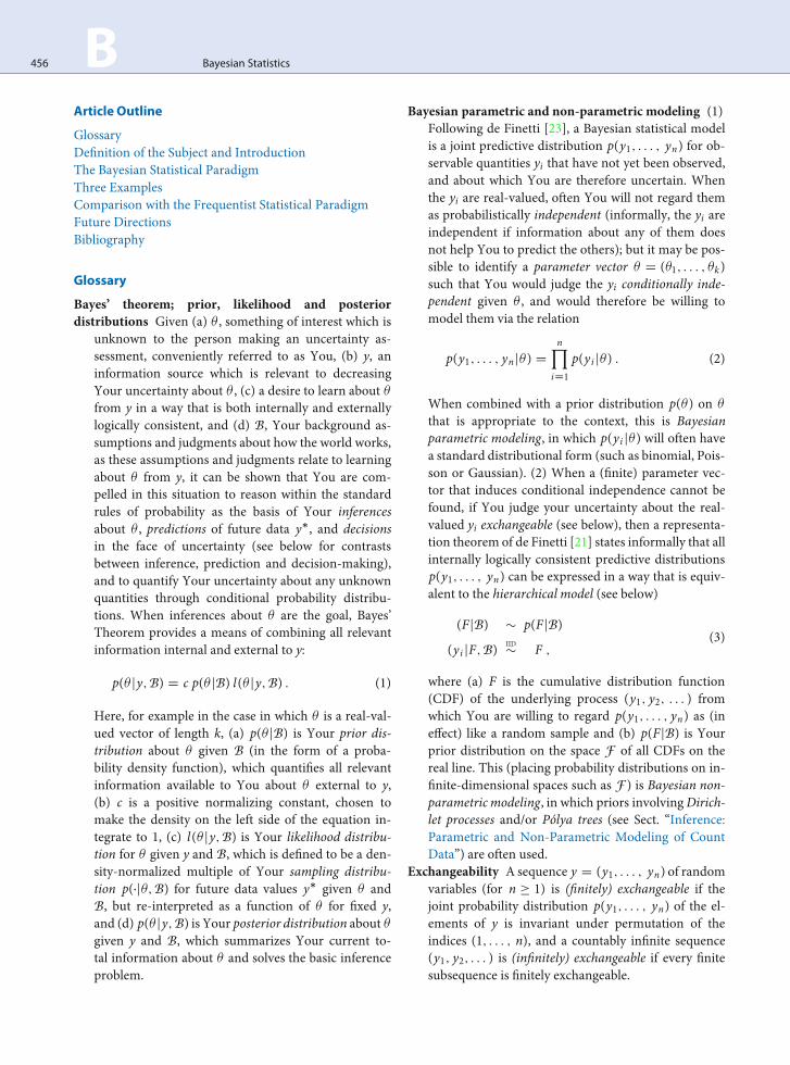
Suppose for illustration that the time period in ques-tion is about four years in length and H is a medium-sizeUS hospital; then there will be about n D 385 heart attackpatients in the data set y. Suppose further that the observedmortality rate at H comes out y D sn / n D 69 / 385 :

D

18%. Figure 1 summarizes the prior-to-posterior updat-ing with this data set and the two priors for Analysts 1(left panel) and 2 (right panel), with ˛ D ˇ D 1 (the Uni-form distribution) for Analyst 2. Even though the twopriors are rather different – Analyst 1’s prior is skewed,with a prior mean of 0.15 and n0

:D 30; Analyst 2’s prior

is flat, with a prior mean of 0.5 and n0 D 2 – it is evi-dent that the posterior distributions are nearly the samein both cases; this is because the data sample size n D 385is so much larger than either of the prior sample sizes, sothat the likelihood information dominates. With both pri-ors the likelihood and posterior distributions are nearlythe same, another consequence of n0 n. For Analyst 1the posterior mean, standard deviation, and 95% centralposterior interval for � are (0:177; 0:00241; 0:142; 0:215),and the corresponding numerical results for Analyst 2are (0:181; 0:00258; 0:144; 0:221); again it is clear that thetwo sets of results are almost identical. With a large sam-ple size, careful elicitation – like that undertaken by Ana-lyst 1 –will often yield results similar to those with a diffuseprior.

The posterior predictive distributionp(ynC1jy1; : : :yn ;B) for the next observation, having observed the first n, isalso straightforward to calculate in closed form with theconjugate prior in this model. It is clear that p(ynC1jy;B)has to be a Bernoulli(��) distribution for some ��, andintuition says that �� should just be the mean ˛�/ (˛� Cˇ�) of the posterior distribution for � given y, in which˛� D ˛ C sn and ˇ� D ˇ C n � sn are the parametersof the Beta posterior. To check this, making use of the factthat the normalizing constant in the Beta(˛; ˇ) family is� (˛ C ˇ) /� (˛)� (ˇ), the second equation in (6) gives

p(ynC1jy1; : : : yn ;B)

D

Z 1

0� ynC1 (1 � �)1�ynC1

� (˛� C ˇ�)� (˛�)� (ˇ�)

�˛��1

� (1 � �)ˇ��1 d�


Bayesian Statistics, Figure 1Prior-to-posterior updating with two prior specifications in the mortality data set (in both panels, prior: long dotted lines; likelihood:short dotted lines; posterior: solid lines). The left and right panels give the updating with the priors for Analysts 1 and 2, respectively

D� (˛� C ˇ�)� (˛�)� (ˇ�)

Z 1

0�˛�CynC1�1

� (1 � �)(ˇ��ynC1C1)�1 d�

D

�� (˛� C ynC1)

� (˛�)

� �� (ˇ� � ynC1 C 1)

� (ˇ�)

�

�

�� (˛� C ˇ�)

� (˛� C ˇ� C 1)

�; (18)

this, combined with the fact that � (x C 1) /� (x) D x forany real x, yields, for example in the case ynC1 D 1,

p(ynC1 D 1jy;B) D�� (˛� C 1)� (˛�)

� �� (˛� C ˇ�)

� (˛� C ˇ� C 1)

�

D˛�

˛� C ˇ�; (19)

confirming intuition.

Inference: Parametric and Non-Parametric Modelingof Count Data

Most elderly people in the Western world say they wouldprefer to spend the end of their lives at home, but manyinstead finish their lives in an institution (a nursing home

or hospital). How can elderly people living in their com-munities be offered health and social services that wouldhelp to prevent institutionalization? Hendriksen et al. [51]conducted an experiment in the 1980s in Denmark to testthe effectiveness of in-home geriatric assessment (IHGA),a form of preventive medicine in which each person’smedical and social needs are assessed and acted upon in-dividually. A total of n D 572 elderly people living in non-institutional settings in a number of villages were random-ized, nC D 287 to a control group, who received standardhealth care, and nT D 285 to a treatment group, who re-ceived standard care plus IHGA. The number of hospital-izations during the two-year life of the study was an out-come of particular interest.

The data are presented and summarized in Table 1. Ev-idently IHGA lowered the mean hospitalization rate pertwo years (for the elderly Danish people in the study, atleast) by (0:944 � 0:768) :D 0:176, which is about an 18%reduction from the control level, a clinically large differ-ence. The question then becomes, in Bayesian inferentiallanguage: what is the posterior distribution for the treat-ment effect in the entire population P of patients judgedexchangeable with those in the study?


Bayesian Statistics, Table 1Distribution of number of hospitalizations in the IHGA study

GroupNumber of Hospitalizations Sample0 1 2 3 4 5 6 7 n Mean Variance

Control 138 77 46 12 8 4 0 2 287 0.944 1.54Treat-ment

147 83 37 13 3 1 1 0 285 0.768 1.02

Continuing to refer to the relevant analyst as You, witha binary outcome variable and no covariates in Sect. “In-ference and Prediction: Binary Outcomes with No Covari-ates” the model arose naturally from a judgment of ex-changeability of Your uncertainty about all n outcomes,but such a judgment of unconditional exchangeabilitywould not be appropriate initially here; to make sucha judgment would be to assert that the treatment and con-trol interventions have the same effect on hospitalization,and it was the point of the study to see if this is true.Here, at least initially, it would be more scientifically ap-propriate to assert exchangeability separately and in par-allel within the two experimental groups, a judgment deFinetti [22] called partial exchangeability and which hasmore recently been referred to as conditional exchangeabil-ity [28,72] given the treatment/control status covariate.

Considering for the moment just the control groupoutcome values Ci ; i D 1; : : : ; nC , and seeking as in Sect.“Inference and Prediction: Binary Outcomes with NoCovariates” to model them via a predictive distribu-tion p(C1; : : : ;CnC jB), de Finetti’s previous representa-tion theorem is not available because the outcomes arereal-valued rather than binary, but he proved [21] anothertheorem for this situation as well: if You’re willing to re-gard (C1; : : : ;CnC ) as the first nC terms in an infinitely ex-changeable sequence (C1;C2; : : : ) of values on R (whichplays the role of the population P, under the control con-dition, in this problem), then to achieve coherence Yourpredictive distribution must be expressible as

p(C1; : : : ;CnC jB) DZ

F

nCY

iD1

F(Ci ) dG(FjB) ; (20)

here (a) F has an interpretation as F(t) D limnC!1 FnC (t),where FnC is the empirical CDF based on (C1; : : : ;CnC );(b) G(FjB) D limnC!1 p(FnC jB), where p(�jB) is Yourjoint probability distribution on (C1;C2; : : : ); and (c) Fis the space of all possible CDFs on R. Equation (20) saysinformally that exchangeability of Your uncertainty aboutan observable process unfolding on the real line is func-tionally equivalent to assuming the Bayesian hierarchical

model

(FjB) � p(FjB)(yi jF;B) IID

� F ;(21)

where p(FjB) is a prior distribution on F . Placing distri-butions on functions, such as CDFs and regression sur-faces, is the topic addressed by the field of Bayesian non-parametric (BNP) modeling [24,80], an area of statisticsthat has recently moved completely into the realm of day-to-day implementation and relevance through advancesin MCMC computational methods. Two rich families ofprior distributions on CDFs about which a wealth of prac-tical experience has recently accumulated include (mix-tures of) Dirichlet processes [32] and Pólya trees [66].

Parametric modeling is of course also possible withthe IHGA data: as noted by Krnjajic et al. [62], whoexplore both parametric and BNP models for data ofthis kind, Poisson modeling is a natural choice, sincethe outcome consists of counts of relatively rare events.The first Poisson model to which one would generallyturn is a fixed-effects model, in which (Ci j C) are IIDPoisson( C ) (i D 1; : : : ; nC D 287) and (Tj j T) are IIDPoisson( T ) ( j D 1; : : : ; nT D 285), with a diffuse prioron ( C ; T ) if little is known, external to the data set,about the underlying hospitalization rates in the controland treatment groups. However, the last two columns ofTable 1 reveal that the sample variance is noticeably largerthan the sample mean in both groups, indicating sub-stantial Poisson over-dispersion. For a second, improved,parametric model this suggests a random-effects Poissonmodel of the form

(Ci j iC)indep� Poisson( iC )

�log( iC )jˇ0C ; �2C

� IID� N(ˇ0C ; �2C ) ;

(22)

and similarly for the treatment group, with diffuse priorsfor (ˇ0C ; �2C ; ˇ0T ; �

2T ). As Krnjajic et al. [62] note, from

a medical point of view this model is more plausible thanthe fixed-effects formulation: each patient in the controlgroup has his/her own latent (unobserved) underlying rateof hospitalization iC , which may well differ from the un-derlying rates of the other control patients because of un-measured differences in factors such as health status at thebeginning of the experiment (and similarly for the treat-ment group).

Model (22), when complemented by its analogue in thetreatment group, specifies a Lognormal mixture of Pois-son distributions for each group and is straightforward tofit by MCMC, but the Gaussian assumption for the mixingdistribution is conventional, not motivated by the under-lying science of the problem, and if the distribution of the


latent variables is not Gaussian – for example, if it is mul-timodal or skewed – model (22) may well lead to incor-rect inferences. Krnjajic et al. [62] therefore also examineseveral BNP models that are centered on the random-ef-fects Poisson model but which permit learning about thetrue underlying distribution of the latent variables insteadof assuming it is Gaussian. One of their models, when ap-plied (for example) to the control group, was

(Ci j iC)indep� Poisson( iC )

�log( iC )jG

� IID� G

(Gj˛;�; �2) � DP[˛ N(�; �2)] :

(23)

Here DP[˛ N(�; �2)] refers to a Dirichlet process priordistribution, on the CDF G of the latent variables, whichis centered at the N(�; �2) model with precision param-eter ˛. Model (23) is an expansion of the random-effectsPoisson model (22) in that the latter is a special case of theformer (obtained by letting ˛ !1). Model expansion isa common Bayesian analytic tool which helps to assess andpropagate model uncertainty: if You are uncertain abouta particular modeling detail, instead of fitting a model thatassumes this detail is correct with probability 1, embed itin a richer model class of which it is a special case, and letthe data tell You about its plausibility.

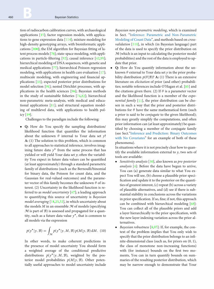
With the IHGA data, models (22) and (23) turnedout to arrive at similar inferential conclusions – in bothcases point estimates of the ratio of the treatment mean tothe control mean were about 0.82 with a posterior stan-dard deviation of about 0.09, and a posterior probabil-ity that the (population) mean ratio was less than 1 ofabout 0.95, so that evidence is strong that IHGA lowersmean hospitalizations not just in the sample but in thecollection P of elderly people to whom it is appropriateto generalize. But the two modeling approaches need notyield similar results: if the latent variable distribution is farfrom Gaussian, model (22) will not be able to adjust tothis violation of one of its basic assumptions. Krnjajic etal. [62] performed a simulation study in which data setswith 300 observations were generated from various Gaus-sian and non-Gaussian latent variable distributions anda variety of parametric and BNP models were fit to the re-sulting count data; Fig. 2 summarizes the prior and pos-terior predictive distributions from models (22; top panel)and (23; bottom panel) with a bimodal latent variable dis-tribution. The parametric Gaussian random-effects modelcannot fit the bimodality on the data scale, but the BNPmodel – even though centered on the Gaussian as the ran-dom-effects distribution – adapts smoothly to the under-lying bimodal reality.

Decision-Making: Variable Selection in GeneralizedLinear Models; Bayesian Model Selection

Variable selection (choosing the “best” subset of predic-tors) in generalized linearmodels is an old problem, datingback at least to the 1960s, and many methods [113] havebeen proposed to try to solve it; but virtually all of themignore an aspect of the problem that can be important: thecost of data collection of the predictors. An example, stud-ied by Fouskakis and Draper [39], which is an elaborationof the problem examined in Sect. “Inference and Predic-tion: Binary Outcomes with No Covariates”, arises in thefield of quality of health care measurement, where patientsickness at admission is often assessed by using logistic re-gression of an outcome, such as mortality within 30 daysof admission, on a fairly large number of sickness indica-tors (on the order of 100) to construct a sickness scale, em-ploying standard variable selection methods (for instance,backward selection from a model with all predictors) tofind an “optimal” subset of 10–20 indicators that predictmortality well. The problem with such benefit-only meth-ods is that they ignore the considerable differences amongthe sickness indicators in the cost of data collection; thisissue is crucial when admission sickness is used to driveprograms (now implemented or under consideration inseveral countries, including the US and UK) that attemptto identify substandard hospitals by comparing observedand expected mortality rates (given admission sickness),because such quality of care investigations are typicallyconducted under cost constraints. When both data-collec-tion cost and accuracy of prediction of 30-day mortalityare considered, a large variable-selection problem arises inwhich the only variables that make it into the final scaleshould be those that achieve a cost-benefit tradeoff.

Variable selection is an example of the broader pro-cess of model selection, in which questions such as “Ismodel M1 better than M2?” and “Is M1 good enough?”arise. These inquiries cannot be addressed, however, with-out first answering a new set of questions: good enough(better than) for what purpose? Specifying this pur-pose [26,57,61,70] identifies model selection as a deci-sion problem that should be approached by constructinga contextually relevant utility function andmaximizing ex-pected utility. Fouskakis and Draper [39] create a utilityfunction, for variable selection in their severity of illnessproblem, with two components that are combined addi-tively: a data-collection component (in monetary units,such as US$), which is simply the negative of the totalamount of money required to collect data on a given setof patients with a given subset of the sickness indicators;and a predictive-accuracy component, in which a method


Bayesian Statistics, Figure 2Prior (open circles) and posterior (solid circles) predictive distributions under models (22) and (23) (top and bottom panels, respec-tively) based on a data set generated from a bimodal latent variable distribution. In each panel, the histogram plots the simulatedcounts

is devised to convert increased predictive accuracy into de-creasedmonetary cost by thinking about the consequencesof labeling a hospital with bad quality of care “good” andvice versa. One aspect of their work, with a data set (froma RAND study: [58]) involving p D 83 sickness indica-tors gathered on a representative sample of n D 2,532 el-derly American patients hospitalized in the period 1980–86 with pneumonia, focused only on the p D 14 variables

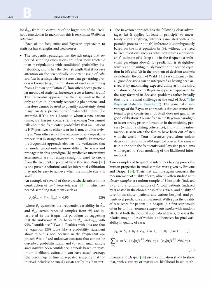
in the original RAND sickness scale; this was chosen be-cause 214 D 16 384 was a small enough number of possi-ble models to do brute-force enumeration of the estimatedexpected utility (EEU) of all themodels. Figure 3 is a paral-lel boxplot of the EEUs of all 16 384 variable subsets, withthe boxplots sorted by the number of variables in eachmodel. The model with no predictors does poorly, with anEEU of about US$�14.5, but from a cost-benefit point of


Bayesian Statistics, Figure 3Estimated expected utility of all 16 384 variable subsets in the quality of care study based on RAND data

view the RAND sickness scale with all 14 variables is evenworse (US$�15.7), because it includes expensive variablesthat do not add much to the predictive power in relationto cheaper variables that predict almost as well. The bestsubsets have 4–6 variables and would save about US$8 perpatient when compared with the entire 14–variable scale;this would amount to significant savings if the observed-versus-expected assessment method were applied widely.

Returning to the general problem of Bayesian modelselection, two cases can be distinguished: situations inwhich the precise purpose to which the model will beput can be specified (as in the variable-selection problemabove), and settings in which at least some of the end usesto which the modeling will be put are not yet known. Inthis second situation it is still helpful to reason in a deci-sion-theoretic way: the hallmark of a good (bad) model isthat it makes good (bad) predictions, so a utility functionbased on predictive accuracy can be a good general-pur-pose choice. With (a) a single sample of data y, (b) a fu-ture data value y�, and (c) two models Mj ( j D 1; 2) forillustration, what is needed is a scoring rule that measuresthe discrepancy between y� and its predictive distribu-tion p(y�jy;Mj;B) under model Mj. It turns out [46,86]that the optimal (impartial, symmetric, proper) scoring

rules are linear functions of log p(y�jy;Mj;B), which hasa simple intuitive motivation: if the predictive distribu-tion is Gaussian, for example, then values of y� close tothe center (in other words, those for which the predic-tion has been good) will receive a greater reward thanthose in the tails. An example [65], in this one-sample set-ting, of a model selection criterion (a) based on prediction,(b) motivated by utility considerations and (c) with goodmodel discrimination properties [29] is the full-sample logscore

LSFS (Mjjy;B) D1n

nX

iD1

log p�(yi jy;Mj;B) ; (24)

which is related to the conditional predictive ordinate cri-terion [90]. Other Bayesianmodel selection criteria in cur-rent use include the following:

� Bayes factors [60]: Bayes’ Theorem, written in oddsform for discriminating between models M1 and M2,says that

p(M1jy;B)p(M2jy;B)

D

�p(M1jB)p(M2jB)

��

�p(yjM1;B)p(yjM2;B)

�; (25)


here the prior odds in favor of M1;

p(M1jB)p(M2jB)

;

are multiplied by the Bayes factor

p(yjM1;B)p(yjM2;B)

to produce the posterior odds

p(M1jy;B)p(M2jy;B)

:

According to the logic of this criterion, models withhigh posterior probability are to be preferred, and if allthe models under consideration are equally plausiblea priori this reduces to preferring models with largerBayes factors in their favor. One problem with this ap-proach is that – in parametric models in which modelMj has parameter vector � j defined on parameter spacej – the integrated likelihoods p(yjMj;B) appearing inthe Bayes factor can be expressed as

p(yjMj;B) DZ

� j

p(yj� j;Mj;B) p(� j jMj;B) d� j

D E(� jjMj;B)�p(yj� j;Mj;B)

�:

(26)

In other words, the numerator and denominator ingre-dients in the Bayes factor are each expressible as expec-tations of likelihood functions with respect to the priordistributions on the model parameters, and if contextsuggests that these priors should be specified diffuselythe resulting Bayes factor can be unstable as a func-tion of precisely how the diffuseness is specified. Var-ious attempts have been made to remedy this insta-bility of Bayes factors (for example, {partial, intrinsic,fractional} Bayes factors, well calibrated priors, conven-tional priors, intrinsic priors, expected posterior pri-ors, . . . ; [9]); all of these methods appear to require anappeal to ad-hockery which is absent from the log scoreapproach.

� Deviance Information Criterion (DIC): Given a para-metric model p(yj� j ;Mj;B), Spiegelhalter et al. [106]define the deviance information criterion (DIC) (byanalogy with other information criteria) to be a trade-off between (a) an estimate of the model lack of fit, asmeasured by the deviance D(� j) (where � j is the poste-rior mean of � j under Mj; for the purpose of DIC, thedeviance of a model [75] is minus twice the logarithm

of the likelihood for that model), and (b) a penalty formodel complexity equal to twice the effective numberof parameters pD j of the model:

DIC(Mjjy;B) D D(� j)C 2 pD j : (27)

When pD j is difficult to read directly from the model(for example, in complex hierarchical models, es-pecially those with random effects), Spiegelhalter etal. motivate the following estimate, which is easy tocompute from standard MCMC output:

pD j D D(� j) � D(� j) ; (28)

in other words, pD j is the difference between the pos-terior mean of the deviance and the deviance evaluatedat the posterior mean of the parameters.DIC is available as an option in several MCMC pack-ages, including WinBUGS [107] and MLwiN [93]. Onedifficulty with DIC is that the MCMC estimate ofpD j can be poor if the marginal posteriors for one ormore parameters (using the parameterization that de-fines the deviance) are far from Gaussian; reparame-terization (onto parameter scales where the posteriorsare approximately Normal) helps but can still lead tomediocre estimates of pD j .

Other notable recent references on the subject of Bayesianvariable selection include Brown et al. [13], who exam-ine multivariate regression in the context of compositionaldata, and George and Foster [43], who use empirical Bayesmethods in the Gaussian linear model.

Comparisonwith the Frequentist Statistical Paradigm

Strengths andWeaknesses of the Two Approaches

Frequentist statistics, which has concentrated mainly oninference, proceeds by (i) thinking of the values in a dataset y as like a random sample from a population P (a setto which it is hoped that conclusions based on the datacan validly be generalized), (ii) specifying a summary �of interest in P (such as the population mean of the out-come variable), (iii) identifying a function � of y that canserve as a reasonable estimate of � , (iv) imagining repeat-ing the random sampling from P to get other data sets yand therefore other values of � , and (v) using the randombehavior of � across these repetitions to make inferentialprobability statements involving � . A leading implemen-tation of the frequentist paradigm [37] is based on usingthe value �MLE that maximizes the likelihood function asthe estimate of � and obtaining a measure of uncertainty


for �MLE from the curvature of the logarithm of the likeli-hood function at its maximum; this ismaximum likelihoodinference.

Each of the frequentist and Bayesian approaches tostatistics has strengths and weaknesses.

� The frequentist paradigm has the advantage that re-peated-sampling calculations are often more tractablethan manipulations with conditional probability dis-tributions, and it has the clear strength that it focusesattention on the scientifically important issue of cali-bration: in settings where the true data-generating pro-cess is known (e. g., in simulations of random samplingfrom a known populationP), how often does a particu-larmethod of statistical inference recover known truth?The frequentist approach has the disadvantage that itonly applies to inherently repeatable phenomena, andtherefore cannot be used to quantify uncertainty aboutmany true-false propositions of real-world interest (forexample, if You are a doctor to whom a new patient(male, say) has just come, strictly speaking You cannottalk about the frequentist probability that this patientis HIV positive; he either is or he is not, and his arriv-ing at Your office is not the outcome of any repeatableprocess that is straightforward to identify). In practicethe frequentist approach also has the weaknesses that(a) model uncertainty is more difficult to assess andpropagate in this paradigm, (b) predictive uncertaintyassessments are not always straightforward to createfrom the frequentist point of view (the bootstrap [31]is one possible solution) and (c) inferential calibrationmay not be easy to achieve when the sample size n issmall.An example of several of these drawbacks arises in theconstruction of confidence intervals [83], in which re-peated-sampling statements such as

Pf (�low < � < �high) D 0:95 (29)

(where Pf quantifies the frequentist variability in �lowand �high across repeated samples from P) are in-terpreted in the frequentist paradigm as suggestingthat the unknown � lies between �low and �high with95% “confidence.” Two difficulties with this are that(a) equation (29) looks like a probability statementabout � but is not, because in the frequentist ap-proach � is a fixed unknown constant that cannot bedescribed probabilistically, and (b) with small samplesizes nominal 95% confidence intervals based on max-imum likelihood estimation can have actual coverage(the percentage of time in repeated sampling that theinterval includes the true �) substantially less than 95%.

� The Bayesian approach has the following clear advan-tages: (a) It applies (at least in principle) to uncer-tainty about anything, whether associated with a re-peatable process or not; (b) inference is unambiguouslybased on the first equation in (6), without the needto face questions such as what constitutes a “reason-able” estimate of � (step (iii) in the frequentist infer-ential paradigm above); (c) prediction is straightfor-wardly and unambiguously based on the second equa-tion in (6); and (d) in the problem of decision analysisa celebrated theorem ofWald [111] says informally thatall good decisions can be interpreted as having been ar-rived at by maximizing expected utility as in the thirdequation of (6), so the Bayesian approach appears to bethe way forward in decision problems rather broadly(but note the final challenge at the end of Sect. “TheBayesian Statistical Paradigm”). The principal disad-vantage of the Bayesian approach is that coherence (in-ternal logical consistency) by itself does not guaranteegood calibration: You are free in the Bayesian paradigmto insert strong prior information in the modeling pro-cess (without violating coherence), and – if this infor-mation is seen after the fact to have been out of stepwith the world – Your inferences, predictions and/ordecisions may also be off-target (of course, the same istrue in the both the frequentist and Bayesian paradigmswith regard to Your modeling of the likelihood infor-mation).

Two examples of frequentist inferences having poor cali-bration properties in small samples were given by Browneand Draper [14]. Their first example again concerns themeasurement of quality of care, which is often studiedwithcluster samples: a random sample of J hospitals (indexedby j) and a random sample of N total patients (indexedby i) nested in the chosen hospitals is taken, and quality ofcare for the chosen patients and various hospital- and pa-tient-level predictors are measured. With yij as the qualityof care score for patient i in hospital j, a first step wouldoften be to fit a variance-components model with randomeffects at both the hospital and patient levels, to assess therelative magnitudes of within- and between-hospital vari-ability in quality of care:

yi j D ˇ0 C uj C ei j; i D 1; : : : ; nj; j D 1; : : : ; J;JX

jD1

njDN; (uj j�2u)

IID� N(0; �2u); (ei jj�

2e )

IID� N(0; �2e ):

(30)

Browne and Draper [14] used a simulation study to showthat, with a variety of maximum-likelihood-based meth-


ods for creating confidence intervals for �2u , the actualcoverage of nominal 95% intervals ranged from 72–94%across realistic sample sizes and true parameter values inthe fields of education and medicine, versus 89–94% forBayesian methods based on diffuse priors.

Their second example involved a re-analysis ofa Guatemalan National Survey of Maternal and ChildHealth [89,97], with three-level data (births nested withinmothers within communities), working with the random-effects logistic regression model

(yi jk j pi jk)indep� Bernoulli

�pi jk

with

logit�pi jk

Dˇ0Cˇ1x1i jkCˇ2x2 jkCˇ3x3kCujkCvk ;

(31)

where yijk is a binary indicator of modern prenatal careor not and where ujk � N(0; �2u) and vk � N(0; �2v )were random effects at the mother and community lev-els (respectively). Simulating data sets with 2 449 birthsby 1 558 women living in 161 communities (as inthe Rodríguez and Goldman study [97]), Browne andDraper [14] showed that things can be even worse for like-lihood-based methods in this model, with actual cover-ages (at nominal 95%) as low as 0–2% for intervals for�2u and �2v , whereas Bayesian methods with diffuse priorsagain produced actual coverages from 89–96%. The tech-nical problem is that the marginal likelihood functions forrandom-effects variances are often heavily skewed, withmaxima at or near 0 even when the true variance is pos-itive; Bayesian methods, which integrate over the likeli-hood function rather thanmaximizing it, can have (much)better small-sample calibration performance as a result.

Some Historical Perspective

The earliest published formal example of an attempt todo statistical inference – to reason backwards from effectsto causes – seems to have been Bayes [5], who definedconditional probability for the first time and noted thatthe result we now call Bayes’ Theorem was a trivial con-sequence of the definition. From the 1760s til the 1920s,all (or almost all) statistical inference was Bayesian, usingthe paradigm that Fisher and others referred to as inverseprobability; prominent Bayesians of this period includedGauss [40], Laplace [64] and Pearson [88]. This Bayesianconsensus changed with the publication of Fisher [37],which laid out a user-friendly program formaximum-like-lihood estimation and inference in a wide variety of prob-lems. Fisher railed against Bayesian inference; his princi-pal objection was that in settings where little was knownabout a parameter (vector) � external to the data, a num-ber of prior distributions could be put forward to quantify

this relative ignorance. He believed passionately in the lateVictorian–Edwardian goal of scientific objectivity, and itbothered him greatly that two analysts with somewhat dif-ferent diffuse priors might obtain somewhat different pos-teriors. (There is a Bayesian account of objectivity: a prob-ability is objective if many different people more or lessagree on its value. An example would be the probability ofdrawing a red ball from an urn known to contain 20 redand 80 white balls, if a sincere attempt is made to thor-oughly mix the balls without looking at them and to drawthe ball in a way that does not tend to favor one ball overanother.)

There are two problems with Fisher’s argument, whichhe never addressed:

1. He would be perfectly correct to raise this objection toBayesian analysis if investigators were often forced todo inference based solely on prior information with nodata, but in practice with even modest sample sizes theposterior is relatively insensitive to the precise man-ner in which diffuseness is specified in the prior, be-cause the likelihood information in such situations isrelatively so much stronger than the prior informa-tion; Sect. “Inference and Prediction: Binary Outcomeswith No Covariates” provides an example of this phe-nomenon.

2. If Fisher had looked at the entire process of inferencewith an engineering eye to sensitivity and stability, hewould have been forced to admit that uncertainty inhow to specify the likelihood function has inferentialconsequences that are often an order of magnitudelarger than those arising from uncertainty in how tospecify the prior. It is an inescapable fact that subjectiv-ity, through assumptions and judgments (such as theform of the likelihood function), is an integral part ofany statistical analysis in problems of realistic complex-ity.

In spite of these unrebutted flaws in Fisher’s objectionsto Bayesian inference, two schools of frequentist infer-ence – one based on Fisher’s maximum-likelihood esti-mation and significance tests [38], the other based on theconfidence intervals and hypothesis tests of Neyman [83]and Neyman and Pearson [84] – came to dominate statis-tical practice from the 1920s at least through the 1980s.One major reason for this was practical: the Bayesianparadigm is based on integrating over the posterior distri-bution, and accurate approximations to high-dimensionalintegrals were not available during the period in question.Fisher’s technology, based on differentiation (to find themaximum and curvature of the logarithm of the likeli-hood function) rather than integration, was a much more


tractable approach for its time. Jeffreys [54], working inthe field of astronomy, and Savage [102] and Lindley [69],building on de Finetti’s results, advocated forcefully for theadoption of Bayesian methods, but prior to the advent ofMCMC techniques (in the late 1980s) Bayesians were of-ten in the position of saying that they knew the best way tosolve statistical problems but the computations were be-yond them. MCMC has removed this practical objectionto the Bayesian paradigm for a wide class of problems.

The increased availability of affordable computers withdecent CPU throughput in the 1980s also helped to over-come one objection raised in Sect. “Strengths and Weak-nesses of the Two Approaches” against likelihood meth-ods, that they can produce poorly-calibrated inferenceswith small samples, through the introduction of the boot-strap by Efron [31] in 1979. At this writing (a) both the fre-quentist and Bayesian paradigms are in vigorous inferen-tial use, with the proportion of Bayesian articles in leadingjournals continuing an increase that began in the 1980s;(b) Bayesian MCMC analyses are often employed to pro-duce meaningful predictive conclusions, with the use ofthe bootstrap increasing for frequentist predictive calibra-tion; and (c) the Bayesian paradigm dominates decisionanalysis.

A Bayesian-Frequentist Fusion

During the 20th century the debate over which paradigmto use was often framed in such a way that it seemedit was necessary to choose one approach and defend itagainst attacks from people who had chosen the other, butthere is nothing that forces an analyst to choose a sin-gle paradigm. Since both approaches have strengths andweaknesses, it seems worthwhile instead to seek a fusionof the two that makes best use of the strengths. Because(a) the Bayesian paradigm appears to be the most flex-ible way so far developed for quantifying all sources ofuncertainty and (b) its main weakness is that coherencedoes not guarantee good calibration, a number of statisti-cians, including Rubin [98], Draper [26], and Little [73],have suggested a fusion in which inferences, predictionsand decisions are formulated using Bayesian methods andthen evaluated for their calibration properties using fre-quentist methods, for example by using Bayesian mod-els to create 95% predictive intervals for observables notused in the modeling process and seeing if approximately95% of these intervals include the actual observed values.Analysts more accustomed to the purely frequentist (like-lihood) paradigm who prefer not to explicitly make useof prior distributions may still find it useful to reason ina Bayesian way, by integrating over the parameter uncer-

tainty in their likelihood functions rather thanmaximizingover it, in order to enjoy the superior calibration proper-ties that integration has been demonstrated to provide.

Future Directions

Since the mid- to late-1980s the Bayesian statistical par-adigm has made significant advances in many fieldsof inquiry, including agriculture, archaeology, astron-omy, bioinformatics, biology, economics, education, en-vironmetrics, finance, health policy, and medicine (seeSect. “The Bayesian Statistical Paradigm” for recent cita-tions of work in many of these disciplines). Three areasof methodological and theoretical research appear particu-larly promising for extending the useful scope of Bayesianwork, as follows:

� Elicitation of prior distributions and utility functions:It is arguable that too much use is made in Bayesiananalysis of diffuse prior distributions, because (a) accu-rate elicitation of non-diffuse priors is hard work and(b) lingering traces still remain of a desire to at least ap-pear to achieve the unattainable Victorian–Edwardiangoal of objectivity, the (false) argument being that theuse of diffuse priors somehow equates to an absenceof subjectivity (see, e. g., the papers by Berger [7] andGoldstein [45] and the ensuing discussion for a vigor-ous debate on this issue). It is also arguable that toomuch emphasis was placed in the 20th century on in-ference at the expense of decision-making, with in-ferential tools such as the Neyman–Pearson hypothe-sis testing machinery (Sect. “Some Historical Perspec-tive”) used incorrectly to make decisions for which theyare not optimal; the main reason for this, as notedin Sect. “Strengths and Weaknesses of the Two Ap-proaches” and “Some Historical Perspective”, is that(a) the frequentist paradigm was dominant from the1920s through the 1980s and (b) the high ground in de-cision theory is dominated by the Bayesian approach.Relevant citations of excellent recent work on elicita-tion of prior distributions and utility functions weregiven in Sect. “The Bayesian Statistical Paradigm”; itis natural to expect that there will be a greater em-phasis on decision theory and non-diffuse prior mod-eling in the future, and elicitation in those fields ofBayesian methodology is an important area of contin-uing research.

� Group decision-making: As noted in Sect. “The Bayes-ian Statistical Paradigm”, maximizing expected utilityis an effective method for decision-making by a singleagent, but when two or more agents are involved in thedecision process this approach cannot be guaranteed to


yield a satisfying solution: there may be conflicts in theagents’ preferences, particularly if their relationship isat least partly adversarial. With three or more possi-ble actions, transitivity of preference – if You prefer ac-tion a1 to a2 and a2 to a3, then You should prefer a1to a3 – is a criterion that any reasonable decision-mak-ing process should obey; informally, a well-known the-orem by Arrow [3] states that even if all of the agents’utility functions obey transitivity, there is no way tocombine their utility functions into a single decision-making process that is guaranteed to respect transitiv-ity. However, Arrow’s theorem is temporally static, inthe sense that the agents do not share their utility func-tions with each other and iterate after doing so, and itassumes that all agents have the same set A of feasi-ble actions. If agents A1 and A2 have action spacesA1andA2 that are not identical and they share the detailsof their utility specification with each other, it is pos-sible that A1 may realize that one of the actions inA2that (s)he had not considered is better than any of theactions inA1 or vice versa; thus a temporally dynamicsolution to the problem posed by Arrow’s theoremmaybe possible, even if A1 and A2 are partially adversarial.This is another important area for new research.

� Bayesian computation: Since the late 1980s, simula-tion-based computation based onMarkov chainMonteCarlo (MCMC) methods has made useful Bayesiananalyses possible in an increasingly broad range of ap-plication areas, and (as noted in Sect. “The BayesianStatistical Paradigm”) increases in computing speedand sophistication of MCMC algorithms have en-hanced this trend significantly. However, if a regres-sion-style data set is visualized as a matrix with n rows(one for each subject of inquiry) and k columns (one foreach variable measured on the subjects), MCMCmeth-ods do not necessarily scale well in either n or k, withthe result that they can be too slow to be of practicaluse with large data sets (e.g, at current desktop com-puting speeds, with n and/or k on the order of 105 orgreater). Improving the scaling of MCMC methods, orfinding a new approach to Bayesian computation thatscales better, is thus a third important area for contin-uing study.

Bibliography1. Abdellaoui M (2000) Parameter-free elicitation of utility and

probability weighting functions. Manag Sci 46:1497–15122. Aleskerov F, BouyssouD,Monjardet B (2007) UtilityMaximiza-

tion, Choice and Preference, 2nd edn. Springer, New York3. Arrow KJ (1963) Social Choice and Individual Values, 2nd edn.

Yale University Press, New Haven CT

4. Barlow RE, Wu AS (1981) Preposterior analysis of Bayes esti-mators of mean life. Biometrika 68:403–410

5. Bayes T (1764) An essay towards solving a problem in the doc-trine of chances. Philos Trans Royal Soc Lond 53:370–418

6. Berger JO (1985) Statistical Decision Theory and BayesianAnalysis. Springer, New York

7. Berger JO (2006) The case for objective Bayesian analysis(with discussion). Bayesian Anal 1:385–472

8. Berger JO, Betro B, Moreno E, Pericchi LR, Ruggeri F, SalinettiG, Wasserman L (eds) (1995) Bayesian Robustness. Instituteof Mathematical Statistics Lecture Notes-Monograph Series,vol 29. IMS, Hayward CA

9. Berger JO, Pericchi LR (2001) Objective Bayesian methodsfor model selection: introduction and comparison. In: LahiriP (ed) Model Selection. Monograph Series, vol 38. Instituteof Mathematical Statistics Lecture Notes Series, Beachwood,pp 135–207

10. Bernardo JM (1979) Reference posterior distributions forBayesian inference (with discussion). J Royal Stat Soc, SeriesB 41:113–147

11. Bernardo JM, Smith AFM (1994) Bayesian Theory. Wiley, NewYork

12. Blavatskyy P (2006) Error propagation in the elicitation of util-ity and probabilityweighting functions. Theory Decis 60:315–334

13. Brown PJ, Vannucci M, Fearn T (1998) Multivariate Bayesianvariable selection and prediction. J Royal Stat Soc, Series B60:627–641

14. Browne WJ, Draper D (2006) A comparison of Bayesian andlikelihoodmethods for fittingmultilevel models (with discus-sion). Bayesian Anal 1:473–550

15. Buck C, Blackwell P (2008) Bayesian construction of radiocar-bon calibration curves (with discussion). In: Case Studies inBayesian Statistics, vol 9. Springer, New York

16. Chipman H, George EI, McCulloch RE (1998) Bayesian CARTmodel search (with discussion). J Am Stat Assoc 93:935–960

17. ChristiansenCL, Morris CN (1997) Hierarchical Poisson regres-sion modeling. J Am Stat Assoc 92:618–632

18. Clyde M, George EI (2004) Model uncertainty. Stat Sci 19:81–94

19. Das S, ChenMH, Kim S, Warren N (2008) A Bayesian structuralequations model for multilevel data with missing responsesandmissing covariates. Bayesian Anal 3:197–224

20. de Finetti B (1930) Funzione caratteristica di un fenomenoaleatorio. Mem R Accad Lincei 4:86–133

21. de Finetti B (1937). La prévision: ses lois logiques, ses sourcessubjectives. Ann Inst H Poincaré 7:1–68 (reprinted in transla-tion as de Finetti B (1980) Foresight: its logical laws, its subjec-tive sources. In: Kyburg HE, Smokler HE (eds) Studies in Sub-jective Probability. Dover, New York, pp 93–158)

22. de Finetti B (1938/1980). Sur la condition d’équivalence par-tielle. Actual Sci Ind 739 (reprinted in translation as de FinettiB (1980) On the condition of partial exchangeability. In: Jef-frey R (ed) Studies in Inductive Logic and Probability. Univer-sity of California Press, Berkeley, pp 193–206)

23. de Finetti B (1970) Teoria delle Probabilità, vol 1 and 2. Eu-naudi, Torino (reprinted in translation as de Finetti B (1974–75) Theory of probability, vol 1 and 2. Wiley, Chichester)

24. Dey D, Müller P, Sinha D (eds) (1998) Practical Nonparametricand Semiparametric Bayesian Statistics. Springer, New York


25. Draper D (1995) Assessment and propagation of model un-certainty (with discussion). J Royal Stat Soc, Series B 57:45–97

26. Draper D (1999) Model uncertainty yes, discrete model aver-aging maybe. Comment on: Hoeting JA, Madigan D, RafteryAE, Volinsky CT (eds) Bayesian model averaging: a tutorial.Stat Sci 14:405–409

27. Draper D (2007) Bayesian multilevel analysis and MCMC. In:de Leeuw J, Meijer E (eds) Handbook of Multilevel Analysis.Springer, New York, pp 31–94

28. Draper D, Hodges J, Mallows C, Pregibon D (1993) Exchange-ability and data analysis (with discussion). J Royal Stat Soc,Series A 156:9–37

29. Draper D, Krnjajic M (2008) Bayesian model specification.Submitted

30. Duran BS, Booker JM (1988) A Bayes sensitivity analysis whenusing the Beta distribution as a prior. IEEE Trans Reliab37:239–247

31. Efron B (1979) Bootstrap methods. Ann Stat 7:1–2632. Ferguson T (1973) A Bayesian analysis of some nonparametric

problems. Ann Stat 1:209–23033. Ferreira MAR, Lee HKH (2007) Multiscale Modeling. Springer,

New York34. Fienberg SE (2006) When did Bayesian inference become

“Bayesian”? Bayesian Anal 1:1–4035. Fishburn PC (1970) Utility Theory for Decision Making. Wiley,

New York36. Fishburn PC (1981) Subjective expected utility: a review of

normative theories. Theory Decis 13:139–19937. Fisher RA (1922) On the mathematical foundations of the-

oretical statistics. Philos Trans Royal Soc Lond, Series A222:309–368

38. Fisher RA (1925) Statistical Methods for Research Workers.Oliver and Boyd, Edinburgh

39. Fouskakis D, Draper D (2008) Comparing stochastic optimiza-tionmethods for variable selection in binary outcome predic-tion, with application to health policy. J Am Stat Assoc, forth-coming

40. Gauss CF (1809) Theoria Motus Corporum Coelestium inSectionibus Conicis Solem Ambientium, vol 2. Perthes andBesser, Hamburg

41. GelfandAE, Smith AFM (1990) Sampling-based approaches tocalculatingmarginal densities. J Am Stat Assoc 85:398–409

42. Gelman A, Meng X-L (2004) Applied Bayesian Modeling andCausal Inference From Incomplete-Data Perspectives. Wiley,New York

43. George EI, Foster DP (2000) Calibration and empirical Bayesvariable selection. Biometrika 87:731–747

44. Gilks WR, Richardson S, Spiegelhalter DJ (eds) (1996) MarkovChainMonte Carlo in Practice. Chapman, New York

45. Goldstein M (2006) Subjective Bayesian analysis: principlesand practice (with discussion). Bayesian Anal 1:385–472

46. Good IJ (1950) Probability and the Weighing of Evidence.Charles Griffin, London

47. Green P (1995) Reversible jump Markov chain Monte carlocomputation and Bayesian model determination. Biometrika82:711–713

48. Hacking I (1984) The Emergence of Probability. UniversityPress, Cambridge

49. Hanson TE, Kottas A, Branscum AJ (2008) Modelling stochas-tic order in the analysis of receiver operating characteristic

data: Bayesian non-parametric approaches. J Royal Stat Soc,Series C (Applied Statistics) 57:207–226

50. Hellwig K, Speckbacher G, Weniges P (2000) Utility maximiza-tion under capital growth constraints. J Math Econ 33:1–12

51. Hendriksen C, Lund E, Stromgard E (1984) Consequences ofassessment and intervention among elderly people: a threeyear randomized controlled trial. Br Med J 289:1522–1524

52. Hoeting JA, Madigan D, Raftery AE, Volinsky CT (1999)Bayesian model averaging: a tutorial. Stat Sci 14:382–417

53. Jaynes ET (2003) Probability Theory: The Logic of Science.Cambridge University Press, Cambridge

54. Jeffreys H (1931) Scientific Inference. Cambridge UniversityPress, Cambridge

55. Jordan MI, Ghahramani Z, Jaakkola TS, Saul L (1999) An intro-duction to variational methods for graphical models. MachLearn 37:183–233

56. Kadane JB (ed) (1996) Bayesian Methods and Ethics in a Clini-cal Trial Design. Wiley, New York

57. Kadane JB, Dickey JM (1980) Bayesian decision theory and thesimplification of models. In: Kmenta J, Ramsey J (eds) Evalua-tion of Econometric Models. Academic Press, New York

58. Kahn K, Rubenstein L, Draper D, Kosecoff J, Rogers W, KeelerE, Brook R (1990) The effects of the DRG-based ProspectivePayment System on quality of care for hospitalized Medicarepatients: An introduction to the series (with discussion). J AmMed Assoc 264:1953–1955

59. Kass RE, Raftery AE (1995) Bayes factors. J Am Stat Assoc90:773–795

60. Kass RE, Wasserman L (1996) The selection of prior distribu-tions by formal rules. J Am Stat Assoc 91:1343–1370

61. Key J, Pericchi LR, Smith AFM (1999) Bayesian model choice:what and why? (with discussion). In: Bernardo JM, Berger JO,Dawid AP, Smith AFM (eds) Bayesian Statistics 6. ClarendonPress, Oxford, pp 343–370

62. Krnjajic M, Kottas A, Draper D (2008) Parametric and non-parametric Bayesian model specification: a case study in-volving models for count data. Comput Stat Data Anal 52:2110–2128

63. Laplace PS (1774) Mémoire sur la probabilité des causes parles évenements. Mém Acad Sci Paris 6:621–656

64. Laplace PS (1812) Théorie Analytique des Probabilités.Courcier, Paris

65. Laud PW, Ibrahim JG (1995) Predictive model selection.J Royal Stat Soc, Series B 57:247–262

66. Lavine M (1992) Some aspects of Pólya tree distributions forstatistical modelling. Ann Stat 20:1222–1235

67. Leamer EE (1978) Specification searches: Ad hoc inferencewith non-experimental data. Wiley, New York

68. Leonard T, Hsu JSJ (1999) Bayesian Methods: An Analysisfor Statisticians and Interdisciplinary Researchers. CambridgeUniversity Press, Cambridge

69. Lindley DV (1965) Introduction to Probability and Statistics.Cambridge University Press, Cambridge

70. Lindley DV (1968) The choice of variables in multiple regres-sion (with discussion). J Royal Stat Soc, Series B 30:31–66

71. Lindley DV (2006) Understanding Uncertainty. Wiley, NewYork

72. Lindley DV, Novick MR (1981) The role of exchangeability ininference. Ann Stat 9:45–58

73. Little RJA (2006) Calibrated Bayes: A Bayes/frequentist road-map. Am Stat 60:213–223


74. Mangel M, Munch SB (2003) Opportunities for Bayesian anal-ysis in the search for sustainable fisheries. ISBA Bulletin10:3–5

75. McCullagh P, Nelder JA (1989) Generalized Linear Models,2nd edn. Chapman, New York

76. Meng XL, van Dyk DA (1997) The EM Algorithm: an old folksong sung to a fast new tune (with discussion). J Royal StatSoc, Series B 59:511–567

77. Merl D, Prado R (2007) Detecting selection in DNA se-quences: Bayesian modelling and inference (with discussion).In: Bernardo JM, Bayarri MJ, Berger JO, Dawid AP, HeckermanD, Smith AFM, West M (eds) Bayesian Statistics 8. UniversityPress, Oxford, pp 1–22

78. Metropolis N, Rosenbluth AW, Rosenbluth MN, Teller AH,Teller E (1953) Equations of state calculations by fast comput-ing machine. J Chem Phys 21:1087–1091

79. Morris CN, Hill J (2000) The Health Insurance Experiment: de-sign using the Finite Selection Model. In: Morton SC, RolphJE (eds) Public Policy and Statistics: Case Studies from RAND.Springer, New York, pp 29–53

80. Müller P, Quintana F (2004) Nonparametric Bayesian dataanalysis. Stat Sci 19:95–110

81. Müller P, Quintana F, Rosner G (2004) Hierarchical meta-anal-ysis over related non-parametric Bayesian models. J RoyalStat Soc, Series B 66:735–749

82. Munch SB, Kottas A, Mangel M (2005) Bayesian nonpara-metric analysis of stock-recruitment relationships. Can J FishAquat Sci 62:1808–1821

83. Neyman J (1937) Outline of a theory of statistical estimationbasedon the classical theory of probability. Philos Trans RoyalSoc Lond A 236:333–380

84. Neyman J, Pearson ES (1928) On the use and interpretationof certain test criteria for purposes of statistical inference.Biometrika 20:175–240

85. O’Hagan A, Buck CE, Daneshkhah A, Eiser JR, Garthwaite PH,Jenkinson DJ, Oakley JE, Rakow T (2006) Uncertain Judge-ments. Eliciting Experts’ Probabilities. Wiley, New York

86. O’Hagan A, Forster J (2004) Bayesian Inference, 2nd edn. In:Kendall’s Advanced Theory of Statistics, vol 2B. Arnold, Lon-don

87. Parmigiani G (2002) Modeling in medical decision-making:A Bayesian approach. Wiley, New York

88. Pearson KP (1895) Mathematical contributions to the the-ory of evolution, II. Skew variation in homogeneous material.Proc Royal Soc Lond 57:257–260

89. Pebley AR, Goldman N (1992) Family, community, ethnicidentity, and the use of formal health care services inGuatemala. Working Paper 92-12. Office of Population Re-search, Princeton

90. Pettit LI (1990) The conditional predictive ordinate for theNormal distribution. J Royal Stat Soc, Series B 52:175–184

91. Pérez JM, Berger JO (2002) Expected posterior prior distribu-tions for model selection. Biometrika 89:491–512

92. Polson NG, Stroud JR, Müller P (2008) Practical filtering withsequential parameter learning. J Royal Stat Soc, Series B70:413–428

93. Rashbash J, Steele F, Browne WJ, Prosser B (2005) A User’sGuide to MLwiN, Version 2.0. Centre for Multilevel Modelling,University of Bristol, Bristol UK; available at www.cmm.bristol.ac.uk Accessed 15 Aug 2008

94. Richardson S, Green PJ (1997) On Bayesian analysis of mix-tures with an unknown number of components (with discus-sion). J Royal Stat Soc, Series B 59:731–792

95. Rios Insua D, Ruggeri F (eds) (2000) Robust Bayesian Analysis.Springer, New York

96. Rodríguez A, Dunston DB, Gelfand AE (2008) The nestedDirichlet process. J Am Stat Assoc, 103, forthcoming

97. Rodríguez G, Goldman N (1995) An assessment of estima-tion procedures for multilevel models with binary responses.J Royal Stat Soc, Series A 158:73–89

98. RubinDB (1984) Bayesianly justifiable and relevant frequencycalculations for the applied statistician. Ann Stat 12:1151–1172

99. Rubin DB (2005) Bayesian inference for causal effects. In: RaoCR, Dey DK (eds) Handbook of Statistics: Bayesian Think-ing, Modeling and Computation, vol 25. Elsevier, Amsterdam,pp 1–16

100. Sabatti C, Lange K (2008) Bayesian Gaussian mixture mod-els for high-density genotyping arrays. J Am Stat Assoc103:89–100

101. Sansó B, Forest CE, Zantedeschi D (2008) Inferring climatesystem properties using a computer model (with discussion).Bayesian Anal 3:1–62

102. Savage LJ (1954) The Foundations of Statistics. Wiley, NewYork

103. Schervish MJ, Seidenfeld T, Kadane JB (1990) State-depen-dent utilities. J Am Stat Assoc 85:840–847

104. Seidou O, Asselin JJ, Ouarda TMBJ (2007) Bayesian multivari-ate linear regression with application to change point mod-els in hydrometeorological variables. In: Water Resources Re-search 43, W08401, doi:10.1029/2005WR004835.

105. Spiegelhalter DJ, Abrams KR, Myles JP (2004) Bayesian Ap-proaches to Clinical Trials and Health-Care Evaluation. Wiley,New York

106. Spiegelhalter DJ, Best NG, Carlin BP, van der Linde A (2002)Bayesian measures of model complexity and fit (with discus-sion). J Royal Stat Soc, Series B 64:583–640

107. Spiegelhalter DJ, ThomasA, Best NG (1999)WinBUGS Version1.2 User Manual. MRC Biostatistics Unit, Cambridge

108. Stephens M (2000) Bayesian analysis of mixture models withan unknown number of components – an alternative to re-versible-jumpmethods. Ann Stat 28:40–74

109. Stigler SM (1986) The History of Statistics: The Measurementof Uncertainty Before 1900. Harvard University Press, Cam-bridge

110. Stone M (1974) Cross-validation choice and assessment ofstatistical predictions (with discussion). J Royal Stat Soc, Se-ries B 36:111–147

111. Wald A (1950) Statistical Decision Functions. Wiley, New York112. Weerahandi S, Zidek JV (1981) Multi-Bayesian statistical deci-

sion theory. J Royal Stat Soc, Series A 144:85–93113. Weisberg S (2005) Applied Linear Regression, 3rd edn. Wiley,

New York114. WestM (2003) Bayesian factor regressionmodels in the “large

p, small n paradigm.” Bayesian Statistics 7:723–732115. West M, Harrison PJ (1997) Bayesian Forecasting and Dy-

namic Models. Springer, New York116. Whitehead J (2006) Using Bayesian decision theory in dose-

escalation studies. In: Chevret S (ed) Statistical Methods forDose-Finding Experiments. Wiley, New York, pp 149–171

http://www.cmm.bristol.ac.uk

http://www.cmm.bristol.ac.uk

http://dx.doi.org/10.1029/2005WR004835.

bayesian statistics - courses - university of california, santa cruz

Documents