some aspects on the arctic energy budget and climatology nils gunnar kvamstø...
TRANSCRIPT
Some aspects on the Arctic energy budget and climatology
Nils Gunnar Kvamstø ([email protected])
Input from Asgeir Sorteberg, Igor Ezau, Vladimir Alexeev and Øyvind Byrkjedal
OUTLINE OF THIS WEEKS LECTURES
1. Arctic Climatology 1
2. Arctic Climatology 2
3. Sea Ice – role, variability, mechanisms
4. Arctic climate variability and climate change
2
,,2
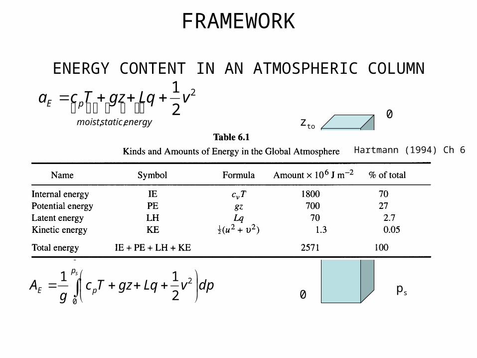
1vLqgzTca
energystaticmoist
pE
dpvLqgzTcg
A
dpag
A
g
dpdz
dzaA
s
s
TOP
p
pE
p
EE
z
EE
0
2
0
0
2
11
1
ps
0ztop
0
FRAMEWORK
ENERGY CONTENT IN AN ATMOSPHERIC COLUMN
Hartmann (1994) Ch 6
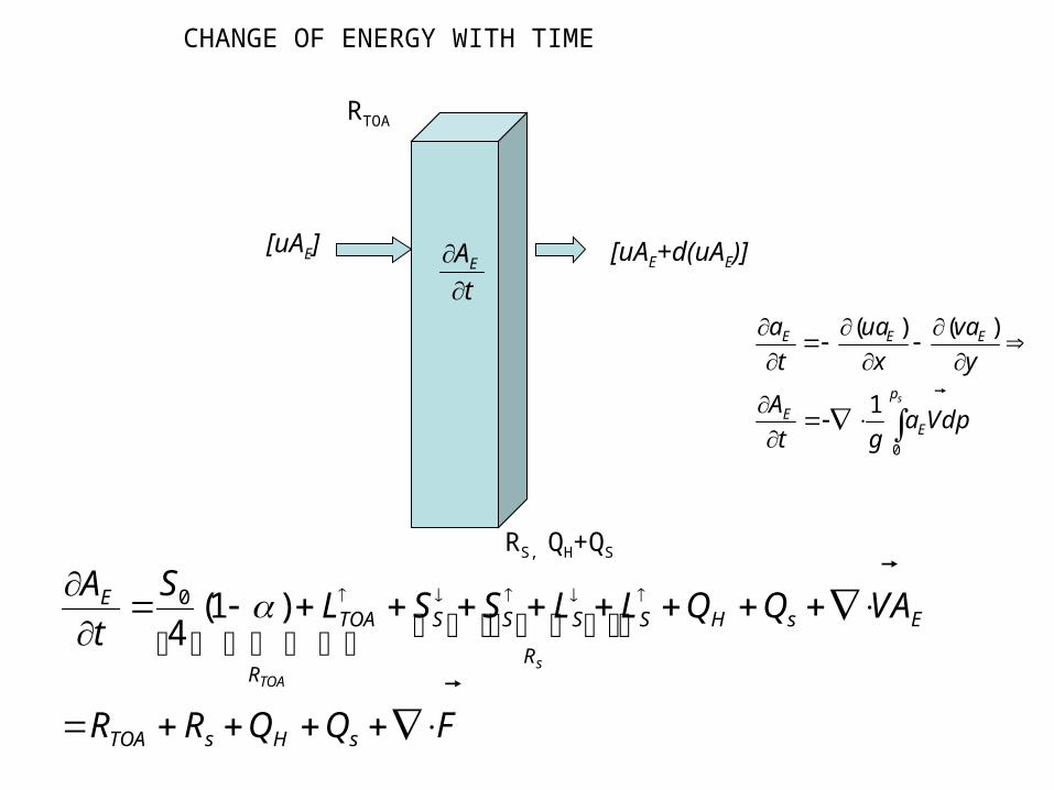
FQQRR
AVQQLLSSLS
t
A
sHsTOA
EsH
R
SSSS
R
TOAE
sTOA
)1(
40
RTOA
RS, QH+QS
[uAE] [uAE+d(uAE)]
dpVagt
A
y
va
x
ua
t
a
sp
EE
EEE
0
1
)()(
t
AE
CHANGE OF ENERGY WITH TIME
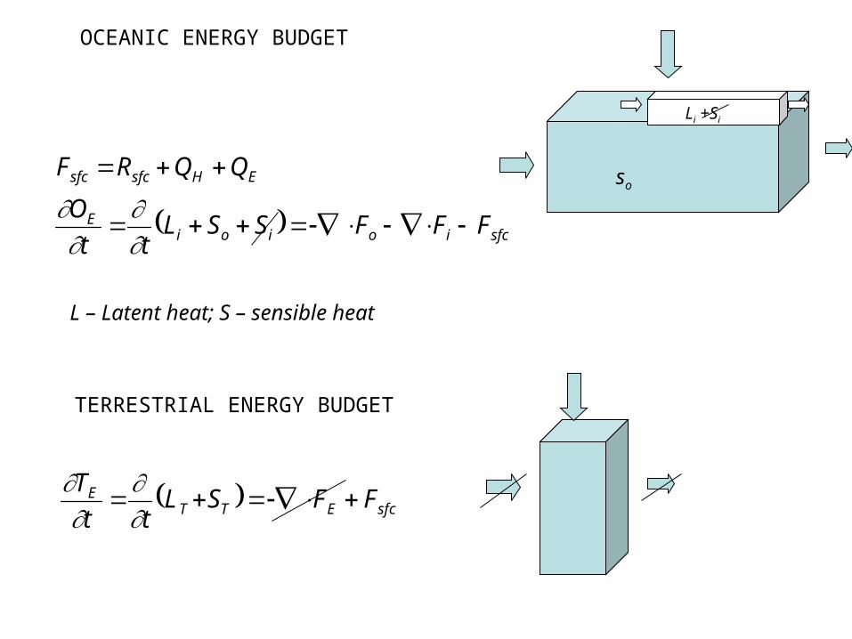
sfcioioiE
EHsfcsfc
FFFSSLtt
O
QQRF
sfcETTE FFSL
tt
T
so
Li +Si
OCEANIC ENERGY BUDGET
TERRESTRIAL ENERGY BUDGET
L – Latent heat; S – sensible heat
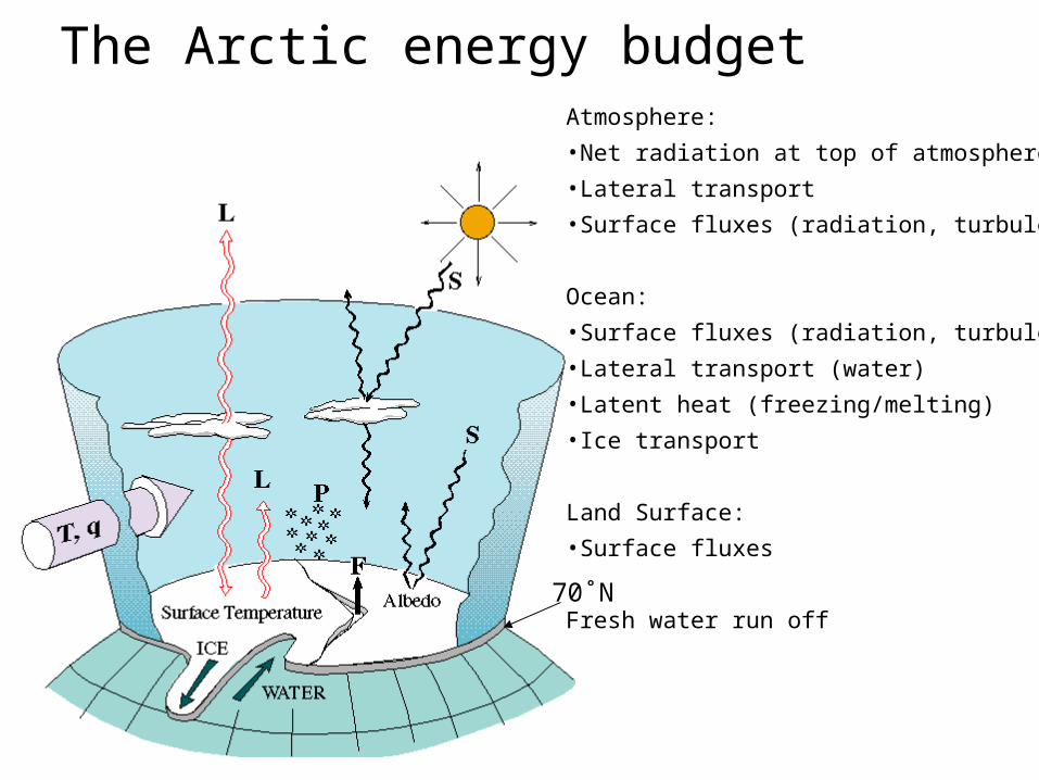
The Arctic energy budget
70˚N
Atmosphere:
•Net radiation at top of atmosphere
•Lateral transport
•Surface fluxes (radiation, turbulence)
Ocean:
•Surface fluxes (radiation, turbulence)
•Lateral transport (water)
•Latent heat (freezing/melting)
•Ice transport
Land Surface:
•Surface fluxes
Fresh water run off
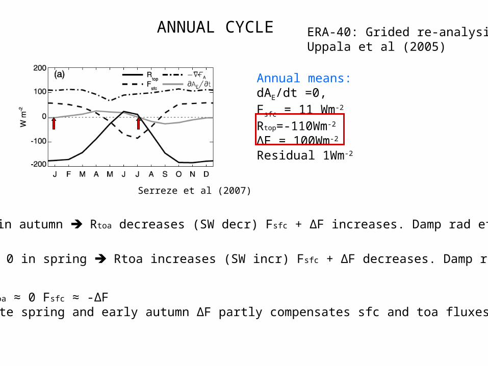
Annual means:dAE/dt =0,Fsfc = 11 Wm-2
Rtop=-110Wm-2
∆F = 100Wm-2
Residual 1Wm-2
∂AE/∂t <0 in autumn Rtoa decreases (SW decr) Fsfc + ∆F increases. Damp rad effect
∂AE/∂t < 0 in spring Rtoa increases (SW incr) Fsfc + ∆F decreases. Damp rad effect
When Rtoa ≈ 0 Fsfc ≈ -∆FBoth late spring and early autumn ∆F partly compensates sfc and toa fluxes
ANNUAL CYCLE
Serreze et al (2007)
ERA-40: Grided re-analysisUppala et al (2005)
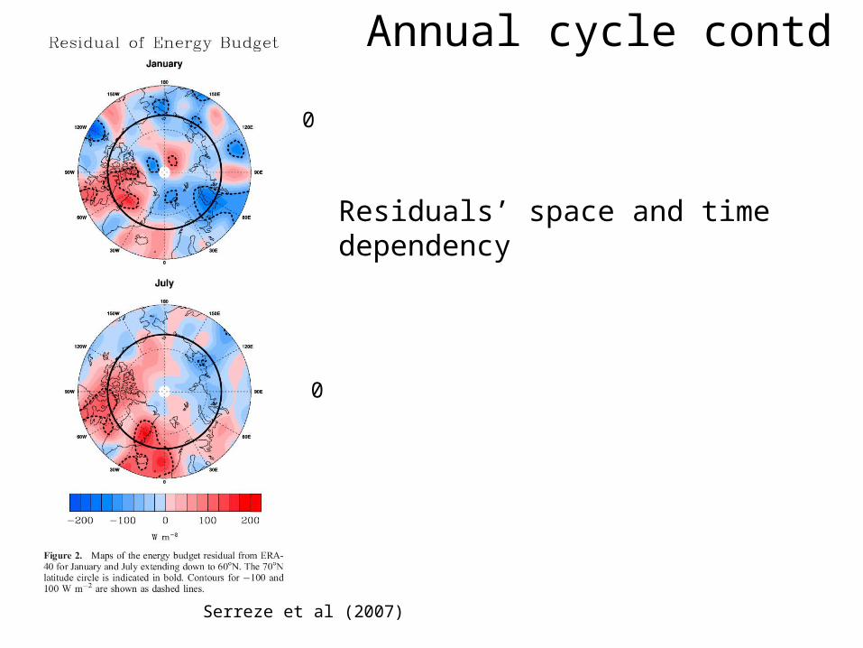
Residuals’ space and time dependency
Serreze et al (2007)
0
0
Annual cycle contd
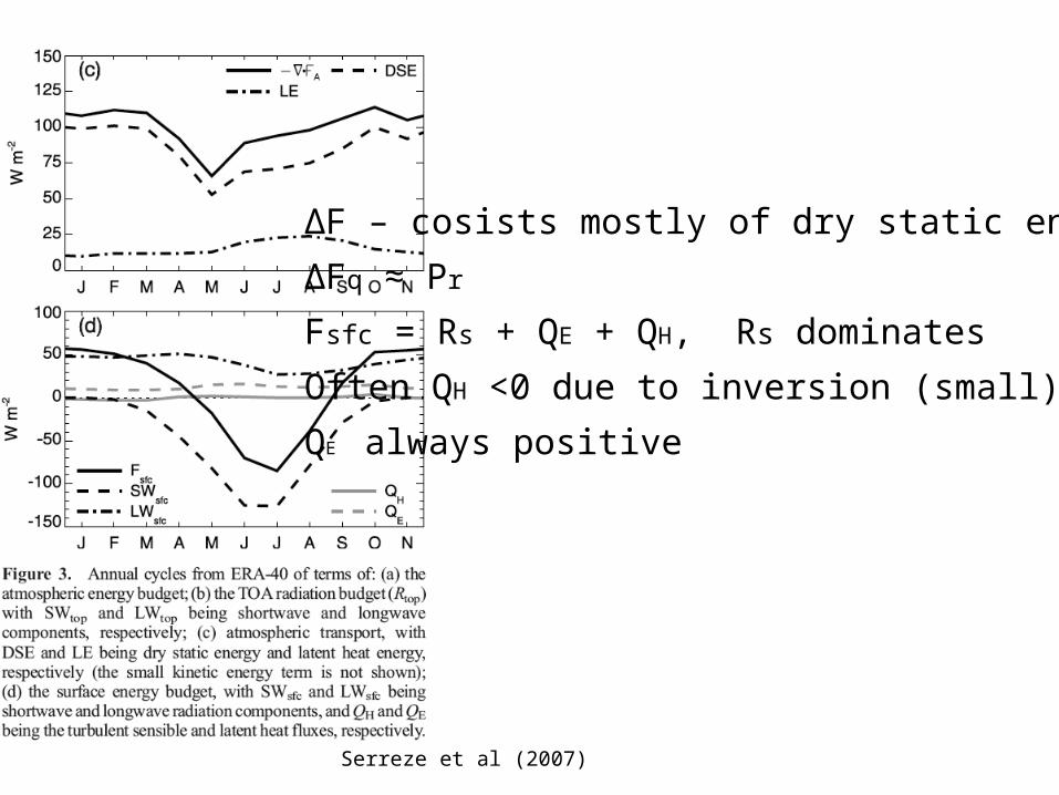
∆F – cosists mostly of dry static energy!
∆Fq ≈ Pr
Fsfc = Rs + QE + QH, Rs dominates
Often QH <0 due to inversion (small)
QE always positive
Serreze et al (2007)
Assessment of ERA40 – comparison with sat.- and obs Data • ∆F well constrained (similar to NCEP)• Fsfc is in the upper range (2.5 – 11)
(1Wm-2 = 0.1m sea ice in 1 yr!!)• Fsfc too high. Inaccurate cloud properties in
ERA40• Excessive Rtop – too high content of
sensible heat• Remember satellite data are inaccurate as
well
Serreze et al (2007)
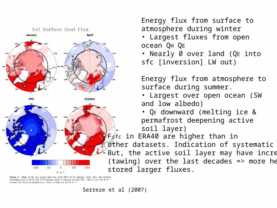
Energy flux from surface to atmosphere during winter• Largest fluxes from open ocean QH QE
• Nearly 0 over land (QE into sfc [inversion] LW out)
Energy flux from atmosphere to surface during summer. • Largest over open ocean (SW and low albedo)• QE downward (melting ice & permafrost deepening active soil layer)
Fsfc in ERA40 are higher than in other datasets. Indication of systematic error.But, the active soil layer may have increased(tawing) over the last decades => more heat stored larger fluxes.
Serreze et al (2007)
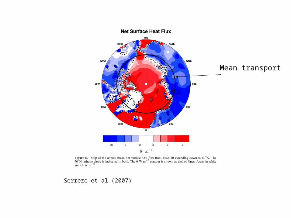
Serreze et al (2007)
Mean transport
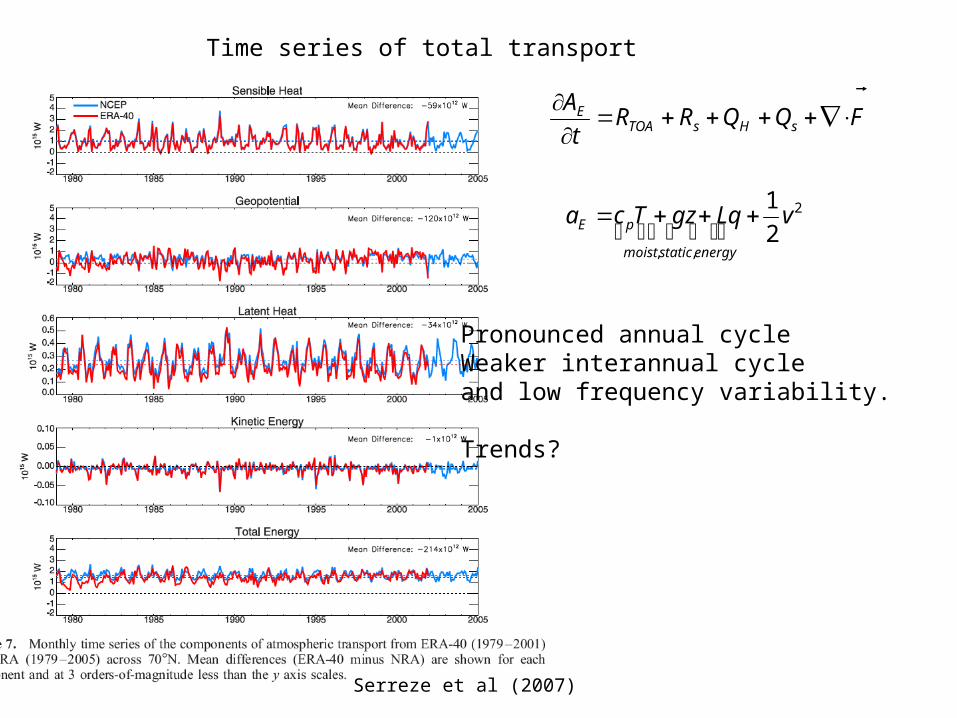
Time series of total transport
Pronounced annual cycleWeaker interannual cycleand low frequency variability.
Trends?
FQQRRt
AsHsTOA
E
2
,,2
1vLqgzTca
energystaticmoist
pE
Serreze et al (2007)
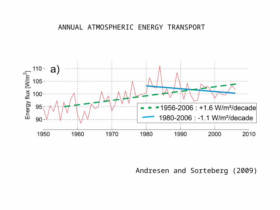
ANNUAL ATMOSPHERIC ENERGY TRANSPORT
Andresen and Sorteberg (2009)
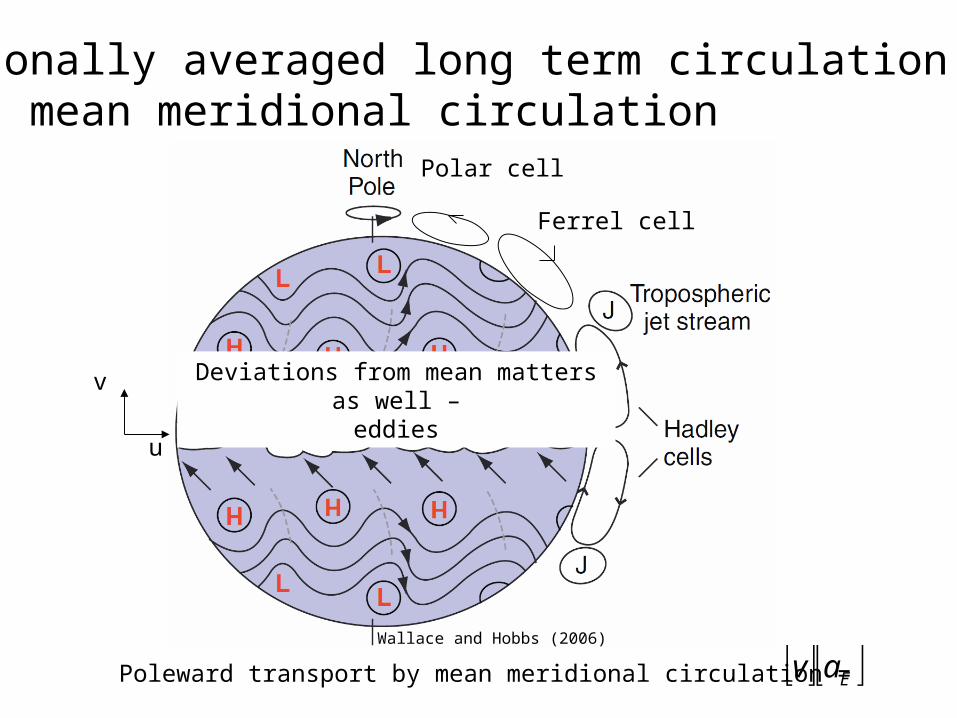
Zonally averaged long term circulation – mean meridional circulation
Ferrel cell
Polar cell
EavPoleward transport by mean meridional circulation =
v
u
Deviations from mean matters as well –eddies
Wallace and Hobbs (2006)
16
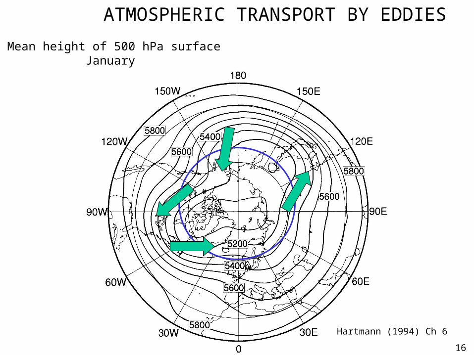
Mean height of 500 hPa surface January
Hartmann (1994) Ch 6
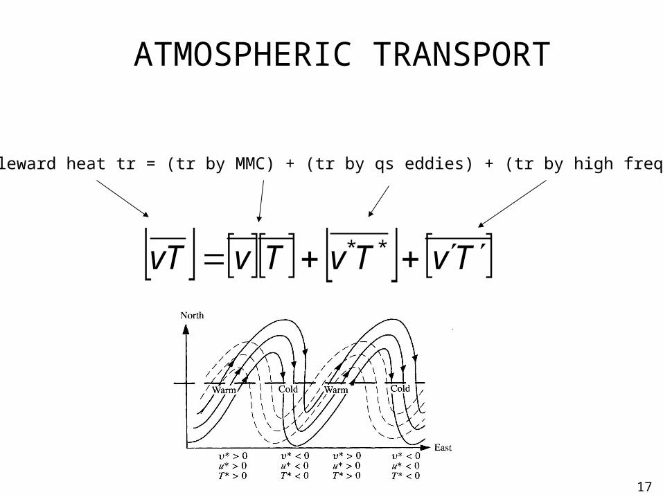
ATMOSPHERIC TRANSPORT BY EDDIES
17
TvTvTvvT **
Total poleward heat tr = (tr by MMC) + (tr by qs eddies) + (tr by high freq eddies)
ATMOSPHERIC TRANSPORT
18
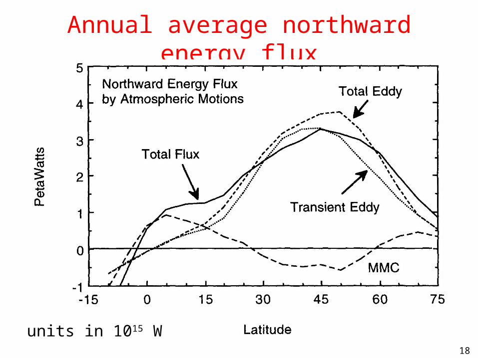
Annual average northward energy flux
units in 1015 W
19
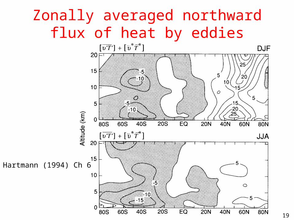
Zonally averaged northward flux of heat by eddies
Hartmann (1994) Ch 6
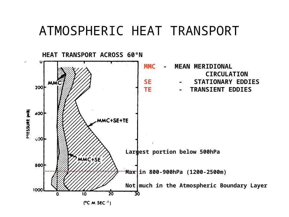
ATMOSPHERIC HEAT TRANSPORT
MMC - MEAN MERIDIONAL CIRCULATIONSE - STATIONARY EDDIESTE - TRANSIENT EDDIES
HEAT TRANSPORT ACROSS 60ºN
Largest portion below 500hPa
Max in 800-900hPa (1200-2500m)
Not much in the Atmospheric Boundary Layer
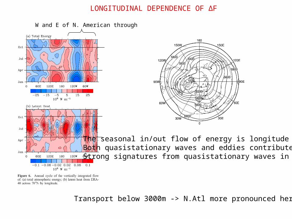
The seasonal in/out flow of energy is longitude dependentBoth quasistationary waves and eddies contribute.Strong signatures from quasistationary waves in figure
W and E of N. American through
Transport below 3000m -> N.Atl more pronounced here
LONGITUDINAL DEPENDENCE OF ΔF
654321
sfcioioiE
EHsfcsfc
FFFSSLtt
O
QQRF
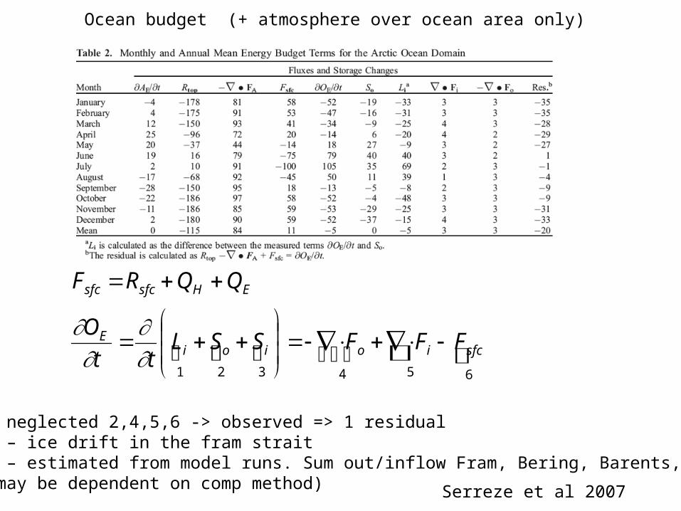
3 neglected 2,4,5,6 -> observed => 1 residual5 – ice drift in the fram strait4 – estimated from model runs. Sum out/inflow Fram, Bering, Barents, Can Arc(may be dependent on comp method)
Ocean budget (+ atmosphere over ocean area only)
Serreze et al 2007
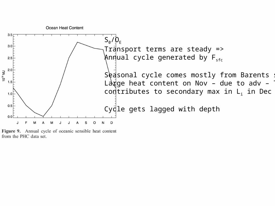
S0/OE
Transport terms are steady => Annual cycle generated by Fsfc
Seasonal cycle comes mostly from Barents sea.Large heat content on Nov – due to adv – This contributes to secondary max in Li in Dec
Cycle gets lagged with depth
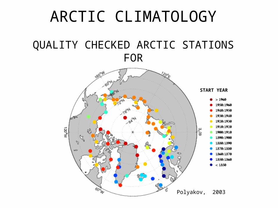
ARCTIC CLIMATOLOGY
QUALITY CHECKED ARCTIC STATIONSFOR
CLIMATE STUDIES
Polyakov, 2003
START YEAR
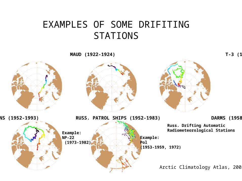
EXAMPLES OF SOME DRIFITING STATIONS
FRAM (1893-1896) MAUD (1922-1924) T-3 (1952-1971)
NP-STATIONS (1952-1993) RUSS. PATROL SHIPS (1952-1983) DARMS (1958-1975)
Example: Pol (1953-1959, 1972)
Example: NP-22 (1973-1982)
Arctic Climatology Atlas, 2002
Russ. Drifting Automatic Radiometeorological Stations
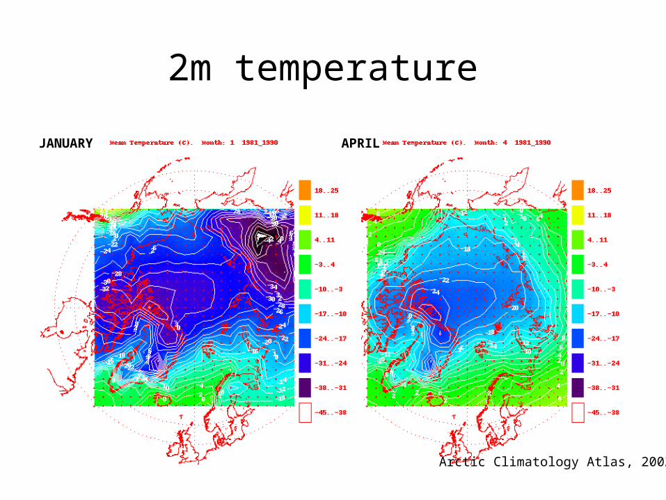
2m temperature
Arctic Climatology Atlas, 2002
JANUARY APRIL
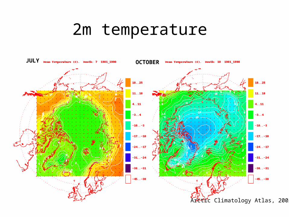
2m temperature
Arctic Climatology Atlas, 2002
JULY OCTOBER
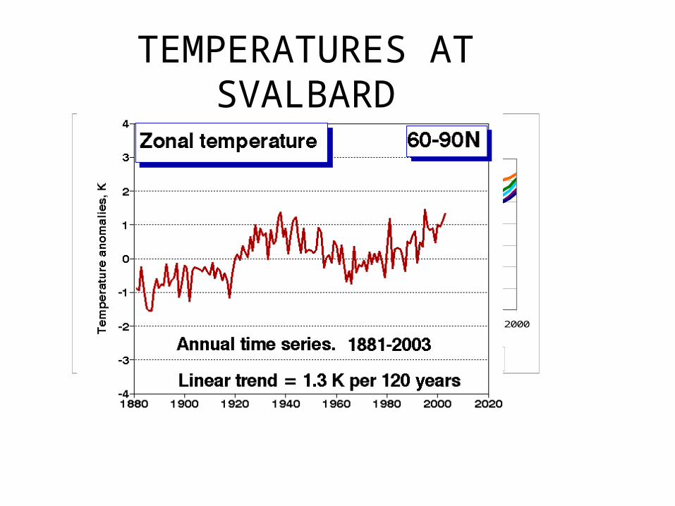
TEMPERATURES AT SVALBARD
Annual
-2.0
-1.5
-1.0
-0.5
0.0
0.5
1.0
1.5
1900 1910 1920 1930 1940 1950 1960 1970 1980 1990 2000
Te
mp
era
ture
(d
eg
C)
Bjørnøya Hopen Svalbard Airport Ny-Ålesund Jan Mayen
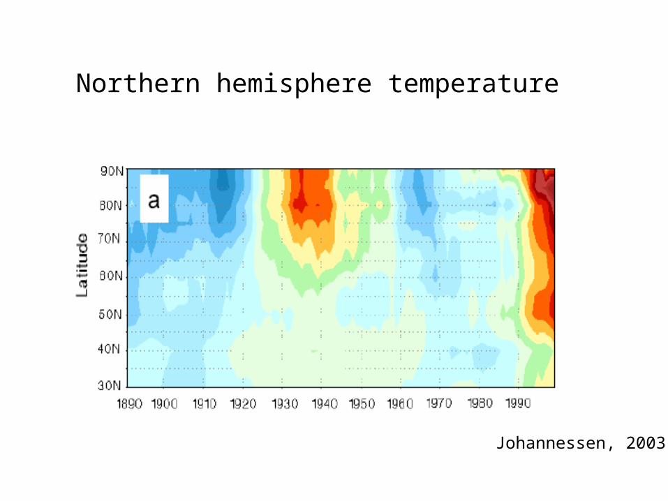
Johannessen, 2003
Northern hemisphere temperature
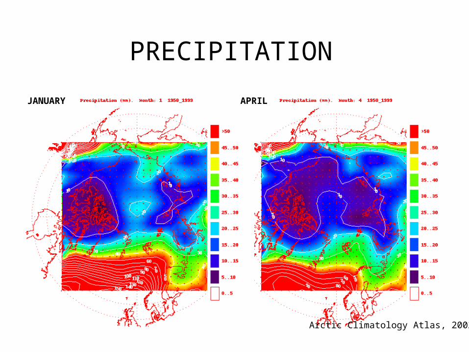
PRECIPITATION
Arctic Climatology Atlas, 2002
JANUARY APRIL
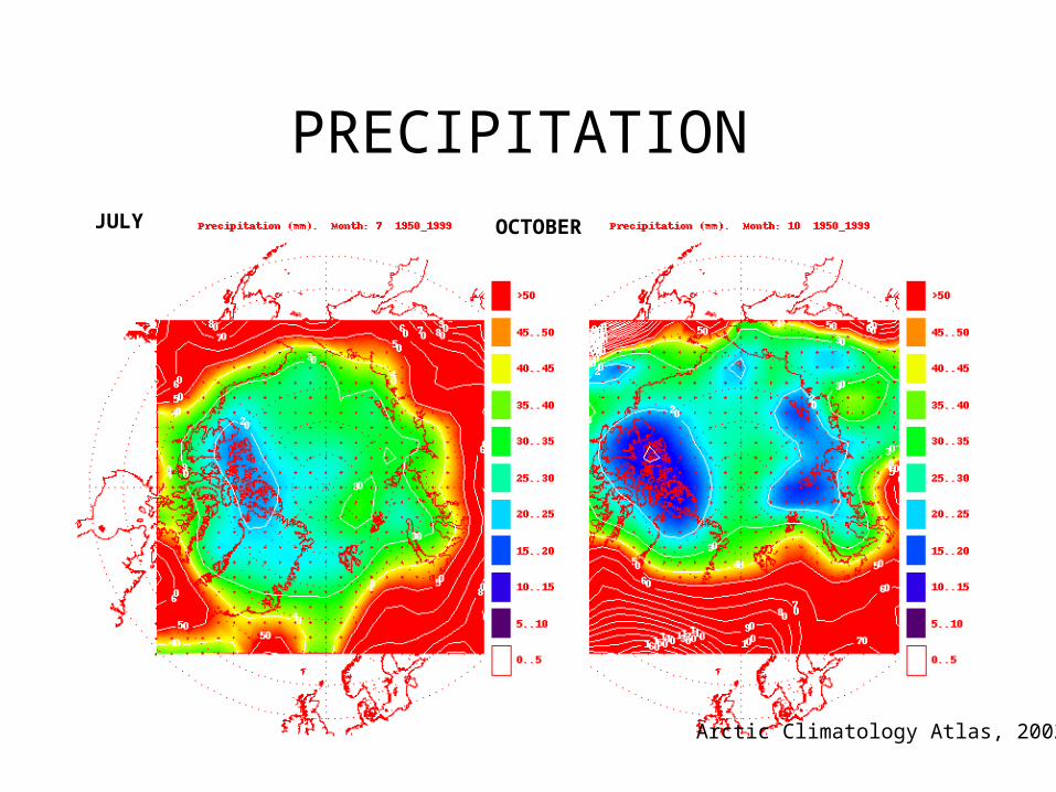
PRECIPITATION
Arctic Climatology Atlas, 2002
JULY OCTOBER
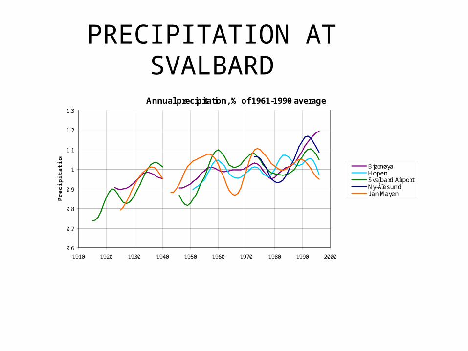
PRECIPITATION AT SVALBARDAnnual precipitation, % of 1961-1990 average
0.6
0.7
0.8
0.9
1
1.1
1.2
1.3
1910 1920 1930 1940 1950 1960 1970 1980 1990 2000
Pre
cip
itat
ion
, % BjørnøyaHopenSvalbard AirportNy-ÅlesundJan Mayen
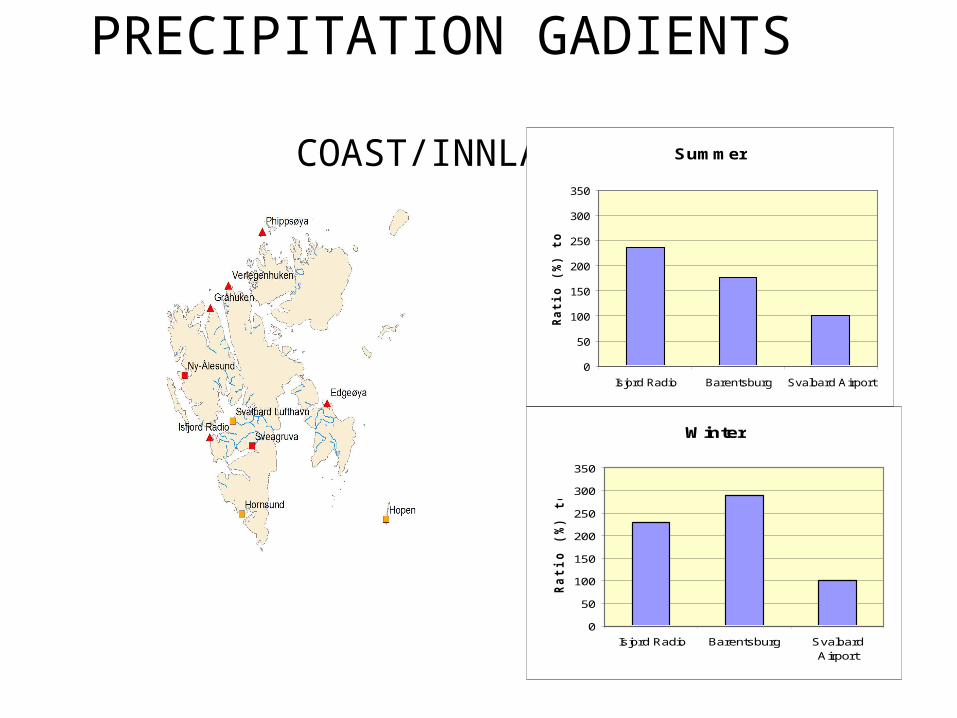
PRECIPITATION GADIENTS COAST/INNLAND
Summer
0
50
100
150
200
250
300
350
Isjord Radio Barentsburg Svalbard Airport
Rati
o (
%)
to S
v.A
p.
Winter
0
50
100
150
200
250
300
350
Isjord Radio Barentsburg SvalbardAirport
Rati
o (
%)
to S
v.A
p.
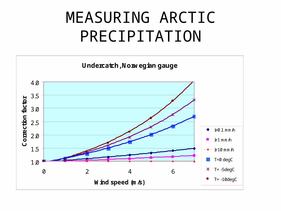
MEASURING ARCTIC PRECIPITATION
Undercatch, Norwegian gauge
1.0
1.5
2.0
2.5
3.0
3.5
4.0
0 2 4 6
Wind speed (m/s)
Co
rre
ctio
n f
acto
r
i=0.1 mm/h
i=1 mm/h
i=10 mm/h
T=0 degC
T= -5degC
T= -10degC
Ekspon. (T= -10degC)Ekspon. (T= -5degC)Ekspon. (T=0degC)Ekspon. (i=0.1mm/h)Ekspon. (i=1mm/h)Ekspon. (i=10mm/h)
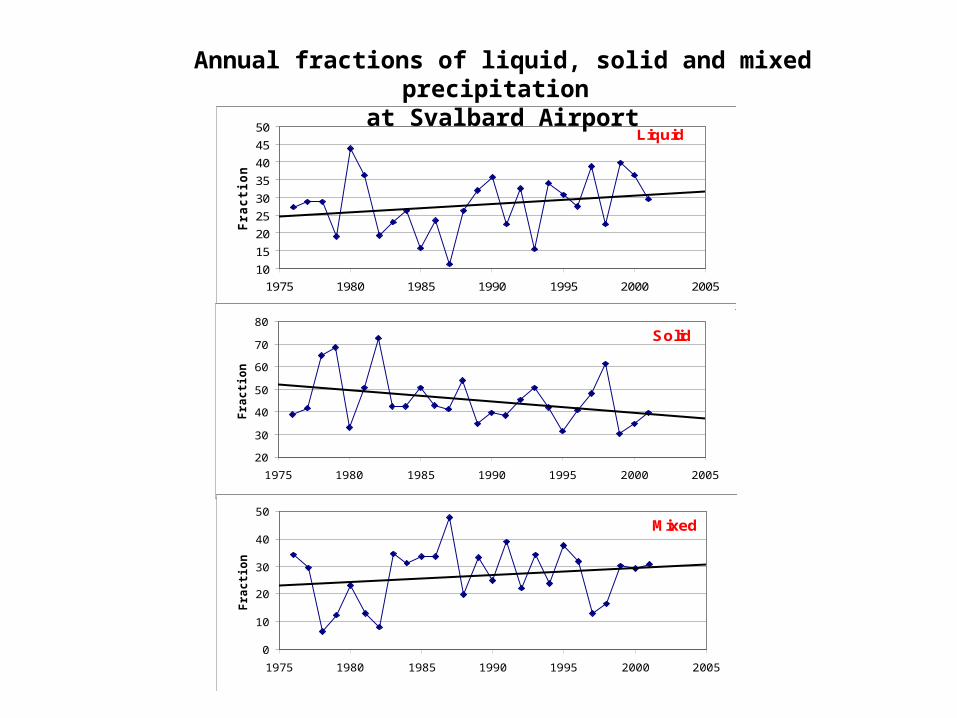
Liquid
10
15
20
25
30
35
40
45
50
1975 1980 1985 1990 1995 2000 2005
Fra
cti
on
(%
)
Solid
20
30
40
50
60
70
80
1975 1980 1985 1990 1995 2000 2005
Fra
cti
on
(%
)
Mixed
0
10
20
30
40
50
1975 1980 1985 1990 1995 2000 2005
Fra
cti
on
(%
)
Annual fractions of liquid, solid and mixed precipitation at Svalbard Airport
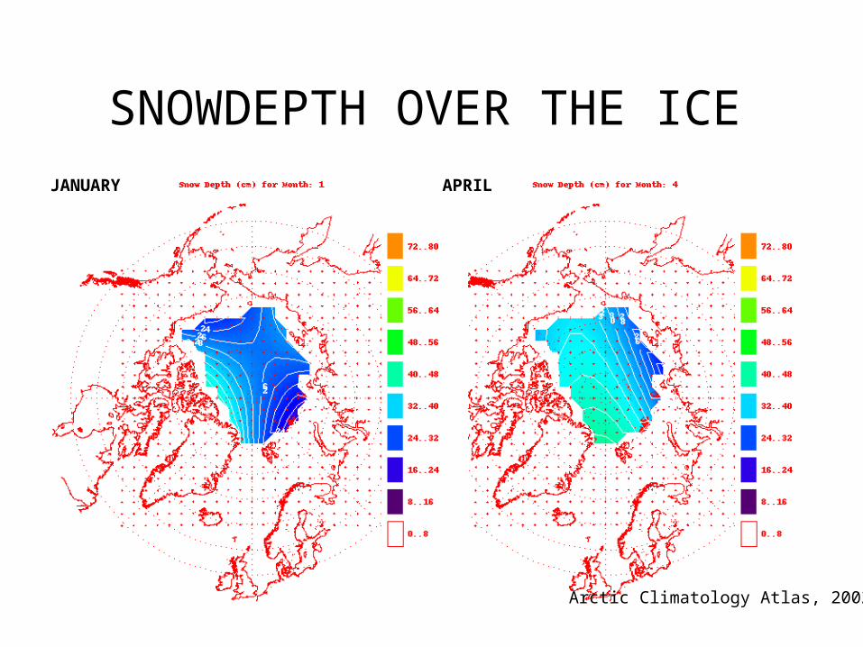
SNOWDEPTH OVER THE ICE
Arctic Climatology Atlas, 2002
JANUARY APRIL
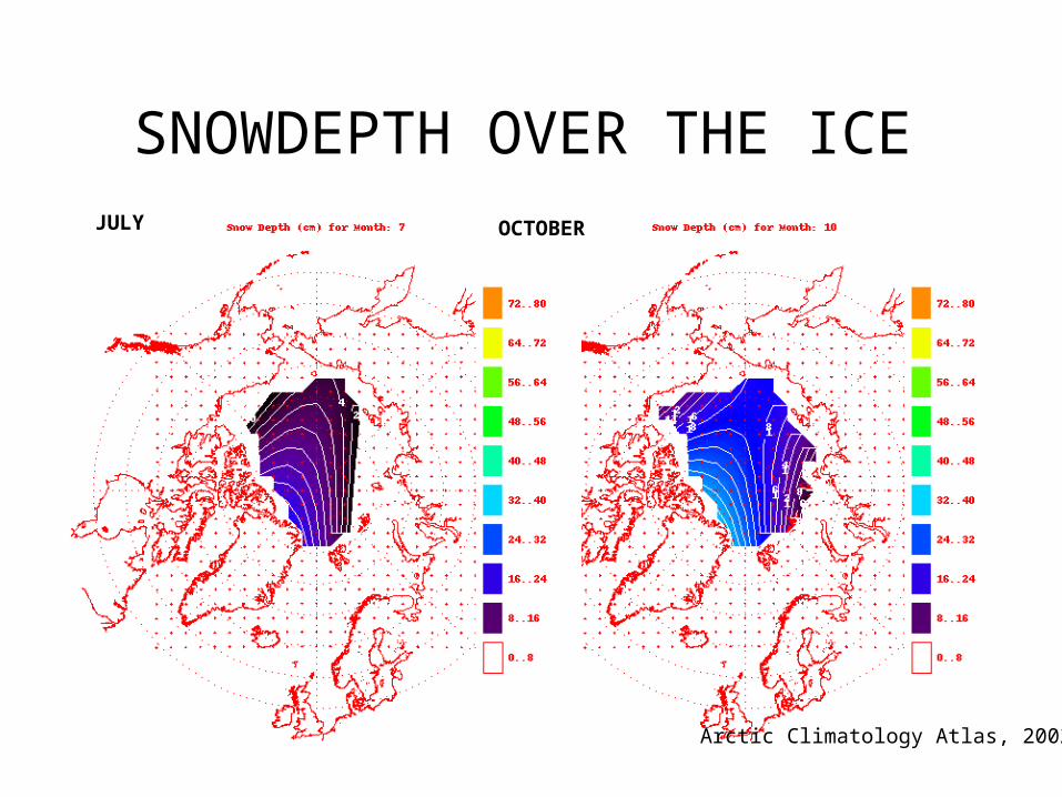
SNOWDEPTH OVER THE ICE
Arctic Climatology Atlas, 2002
JULY OCTOBER
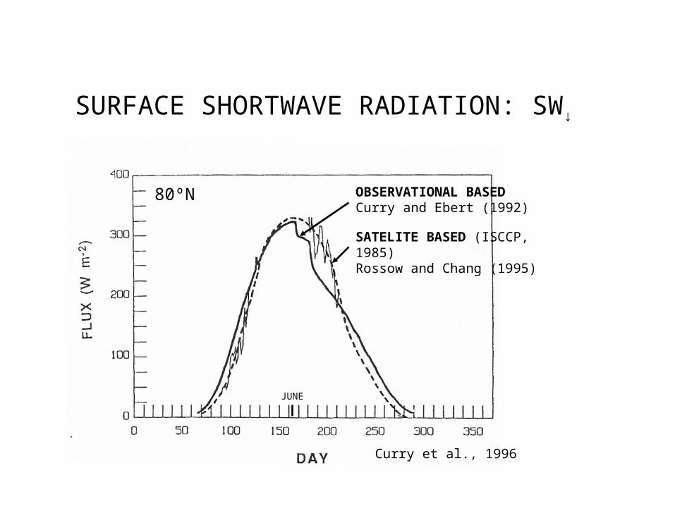
SURFACE SHORTWAVE RADIATION: SW↓
Curry et al., 1996
OBSERVATIONAL BASED Curry and Ebert (1992)
SATELITE BASED (ISCCP, 1985) Rossow and Chang (1995)
JUNE
80ºN
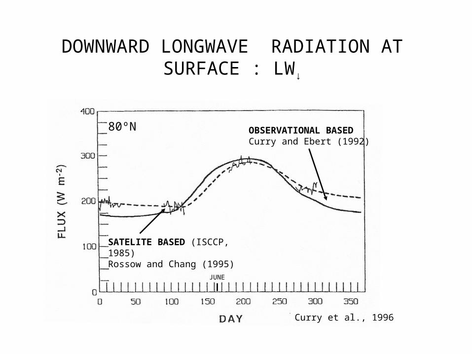
DOWNWARD LONGWAVE RADIATION AT SURFACE : LW↓
Curry et al., 1996
OBSERVATIONAL BASED Curry and Ebert (1992)
SATELITE BASED (ISCCP, 1985) Rossow and Chang (1995)
JUNE
80ºN
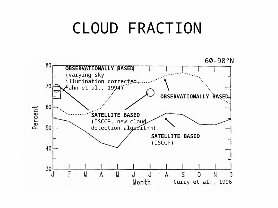
CLOUD FRACTION
Curry et al., 1996
SATELLITE BASED (ISCCP)
60-90ºN
OBSERVATIONALLY BASED
OBSERVATIONALLY BASED(varying sky illumination corrected, Hahn et al., 1994)
SATELLITE BASED (ISCCP, new cloud detection algorithm)
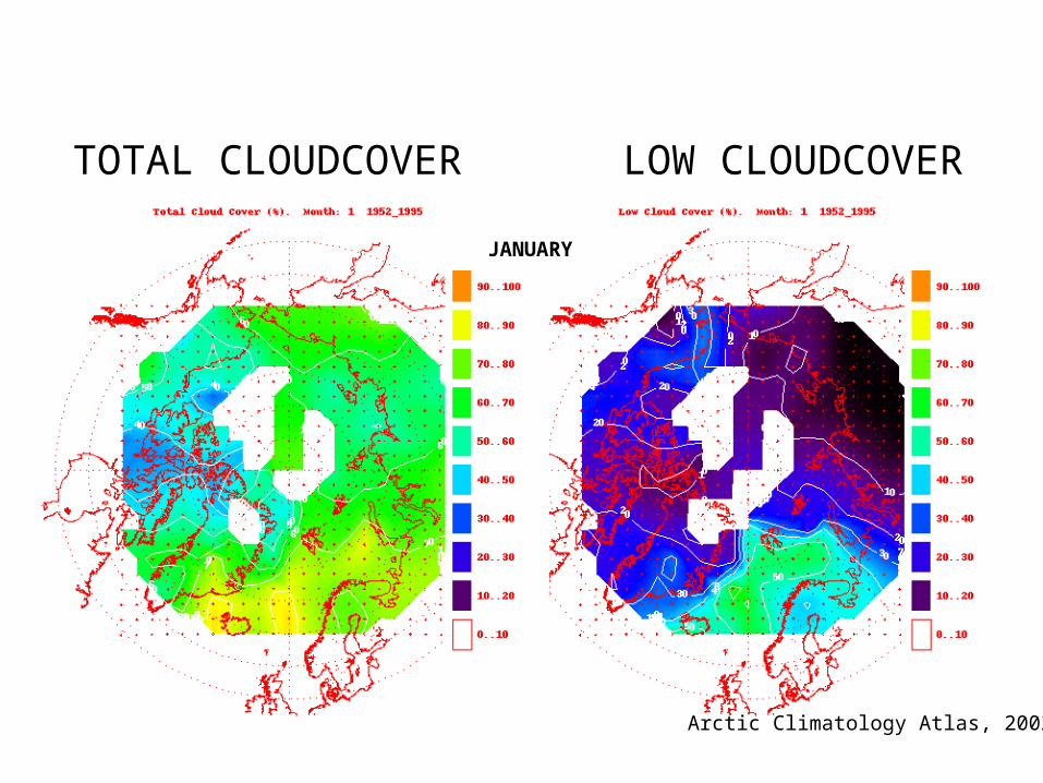
TOTAL CLOUDCOVER
APRIL
Arctic Climatology Atlas, 2002
JANUARY
LOW CLOUDCOVER
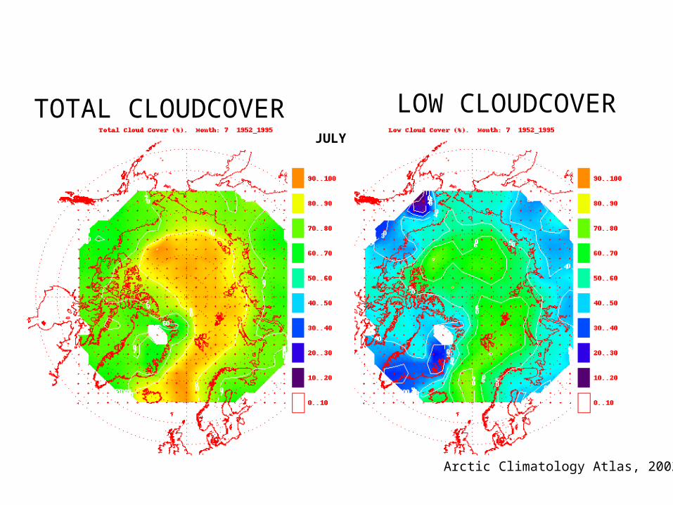
TOTAL CLOUDCOVER
Arctic Climatology Atlas, 2002
JULY
LOW CLOUDCOVER
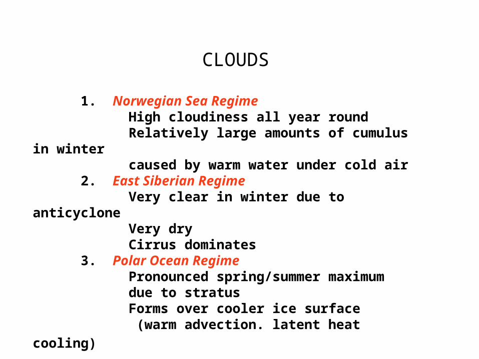
CLOUDS
1. Norwegian Sea RegimeHigh cloudiness all year roundRelatively large amounts of cumulus in winter caused by warm water under cold air
2. East Siberian RegimeVery clear in winter due to anticycloneVery dryCirrus dominates
3. Polar Ocean RegimePronounced spring/summer maximum due to stratusForms over cooler ice surface
(warm advection. latent heat cooling)
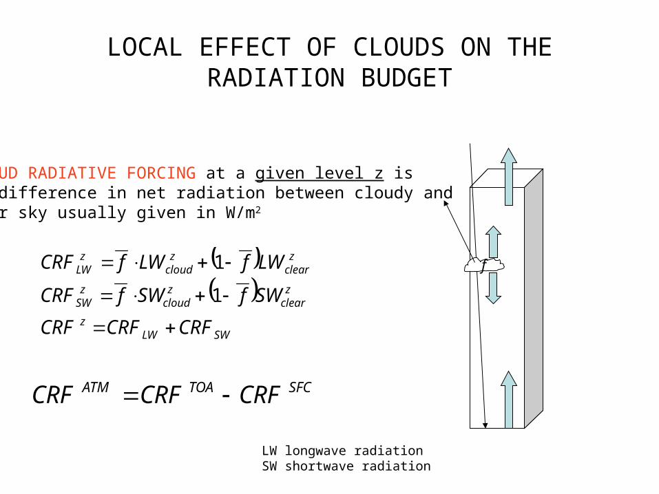
LOCAL EFFECT OF CLOUDS ON THE RADIATION BUDGET
SWLW
z
zclear
zcloud
zSW
zclear
zcloud
zLW
CRFCRFCRF
SWfSWfCRF
LWfLWfCRF
1
1
CLOUD RADIATIVE FORCING at a given level z is the difference in net radiation between cloudy and clear sky usually given in W/m2
LW longwave radiationSW shortwave radiation
f
SFCTOAATM CRFCRFCRF
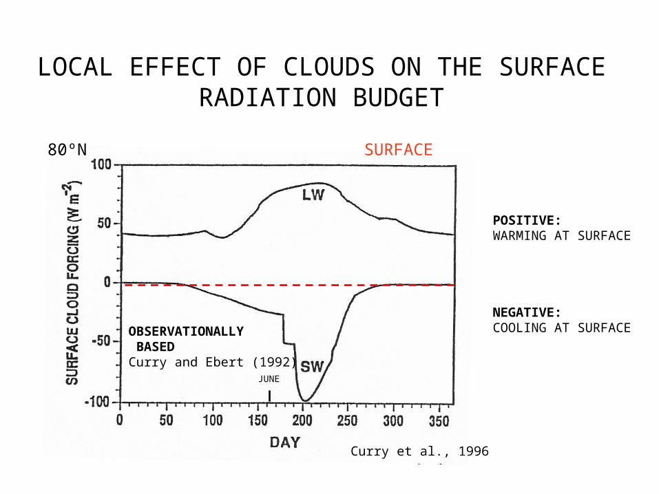
LOCAL EFFECT OF CLOUDS ON THE SURFACE RADIATION BUDGET
Curry et al., 1996
JUNE
80ºN SURFACE
OBSERVATIONALLY BASED Curry and Ebert (1992)
POSITIVE: WARMING AT SURFACE
NEGATIVE: COOLING AT SURFACE
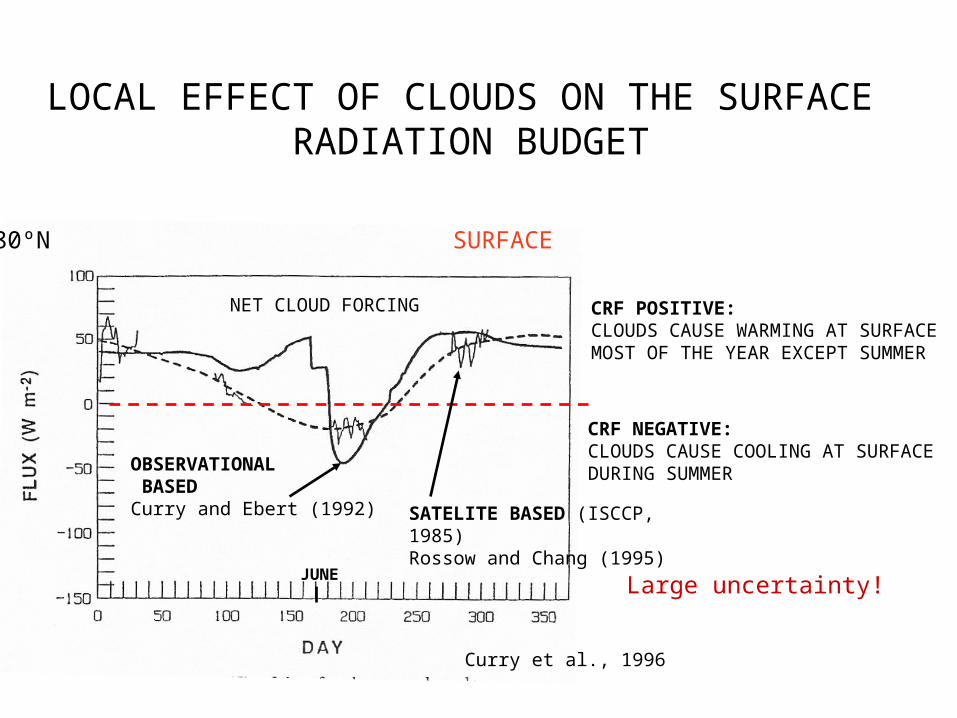
LOCAL EFFECT OF CLOUDS ON THE SURFACE RADIATION BUDGET
Curry et al., 1996
JUNE
80ºN SURFACE
OBSERVATIONAL BASED Curry and Ebert (1992) SATELITE BASED (ISCCP, 1985)
Rossow and Chang (1995)
NET CLOUD FORCING CRF POSITIVE: CLOUDS CAUSE WARMING AT SURFACEMOST OF THE YEAR EXCEPT SUMMER
CRF NEGATIVE: CLOUDS CAUSE COOLING AT SURFACEDURING SUMMER
Large uncertainty!
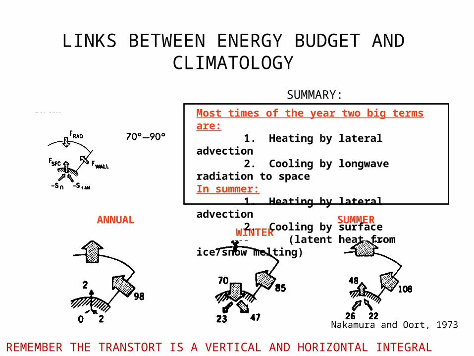
LINKS BETWEEN ENERGY BUDGET AND CLIMATOLOGY
Nakamura and Oort, 1973
ANNUAL SUMMER WINTER
Most times of the year two big terms are:1. Heating by lateral advection 2. Cooling by longwave radiation to space
In summer:1. Heating by lateral advection2. Cooling by surface (latent heat from ice/snow melting)
REMEMBER THE TRANSTORT IS A VERTICAL AND HORIZONTAL INTEGRAL
SUMMARY:
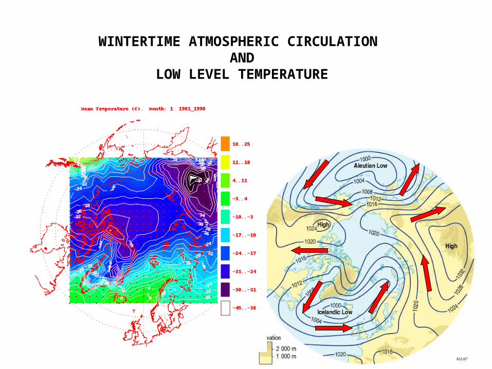
WINTERTIME ATMOSPHERIC CIRCULATION AND
LOW LEVEL TEMPERATURE
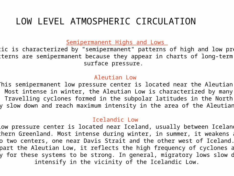
LOW LEVEL ATMOSPHERIC CIRCULATION
Semipermanent Highs and Lows The Arctic is characterized by "semipermanent" patterns of high and low pressure.
These patterns are semipermanent because they appear in charts of long-term average surface pressure.
Aleutian Low This semipermanent low pressure center is located near the Aleutian
Islands. Most intense in winter, the Aleutian Low is characterized by many strong cyclones. Travelling cyclones formed in the subpolar latitudes in the North Pacific usually slow down and reach maximum intensity in the area of the Aleutian Low.
Icelandic Low This low pressure center is located near Iceland, usually between Iceland and southern Greenland. Most intense during winter, in summer, it weakens and
splits into two centers, one near Davis Strait and the other west of Iceland. Like its counterpart the Aleutian Low, it reflects the high frequency of cyclones and the
tendency for these systems to be strong. In general, migratory lows slow down and intensify in the vicinity of the Icelandic Low.
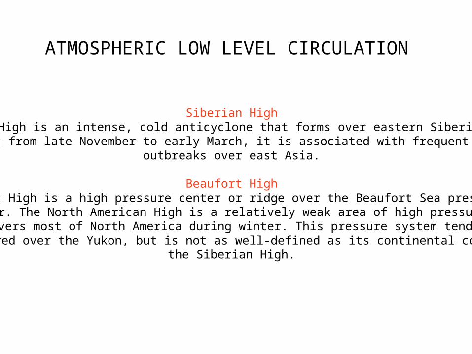
ATMOSPHERIC LOW LEVEL CIRCULATION
Siberian High
The Siberian High is an intense, cold anticyclone that forms over eastern Siberia in winter. Prevailing from late November to early March, it is associated with frequent cold air
outbreaks over east Asia.
Beaufort High The Beaufort High is a high pressure center or ridge over the Beaufort Sea present mainly
in winter. The North American High is a relatively weak area of high pressure that covers most of North America during winter. This pressure system tends
to be centered over the Yukon, but is not as well-defined as its continental counterpart, the Siberian High.
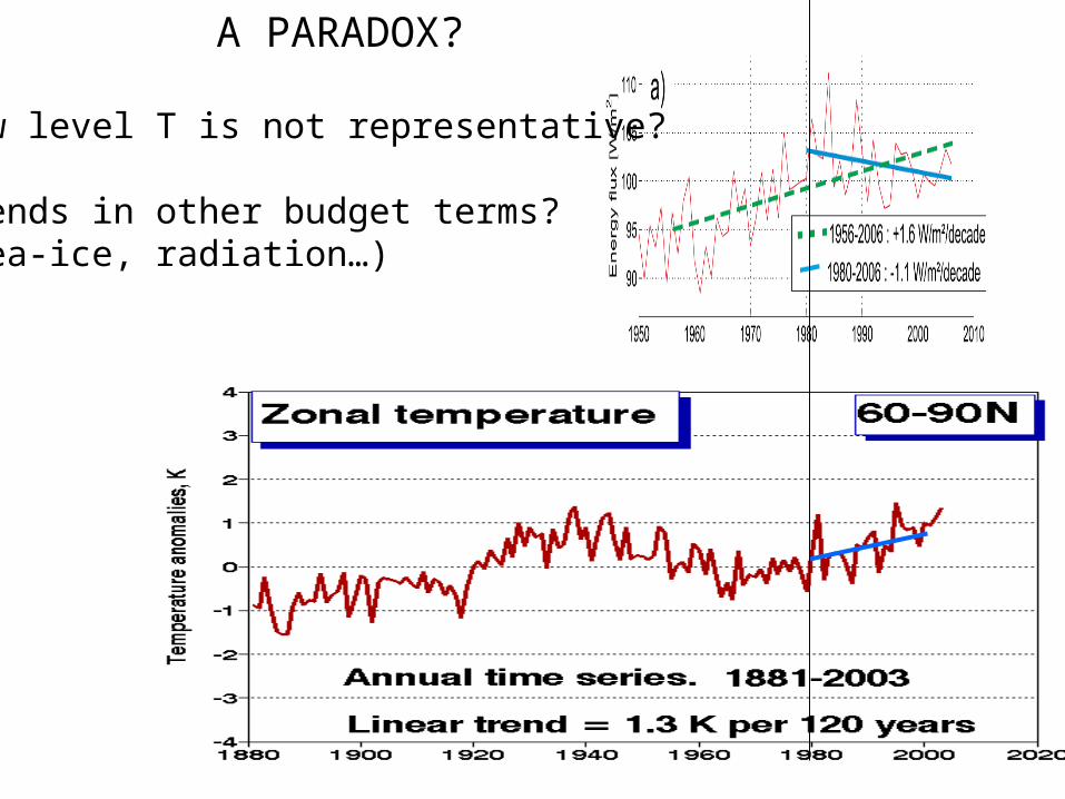
Low level T is not representative?
Trends in other budget terms?(sea-ice, radiation…)
A PARADOX?
HOW WELL DO WE KNOW THE SURFACE RADIATION BUDGET?
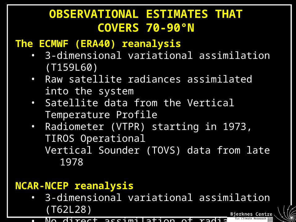
OBSERVATIONAL ESTIMATES THATCOVERS 70-90°N
The ECMWF (ERA40) reanalysis • 3-dimensional variational assimilation (T159L60)• Raw satellite radiances assimilated into the system• Satellite data from the Vertical Temperature Profile• Radiometer (VTPR) starting in 1973, TIROS Operational
Vertical Sounder (TOVS) data from late 1978
NCAR-NCEP reanalysis • 3-dimensional variational assimilation (T62L28)• No direct assimilation of radiative fluxes.• Estimate the vertical temperature and humidity profiles
through a series of empirical and statistical relationships• Satellite data from TIROS TOVS data from late 1978
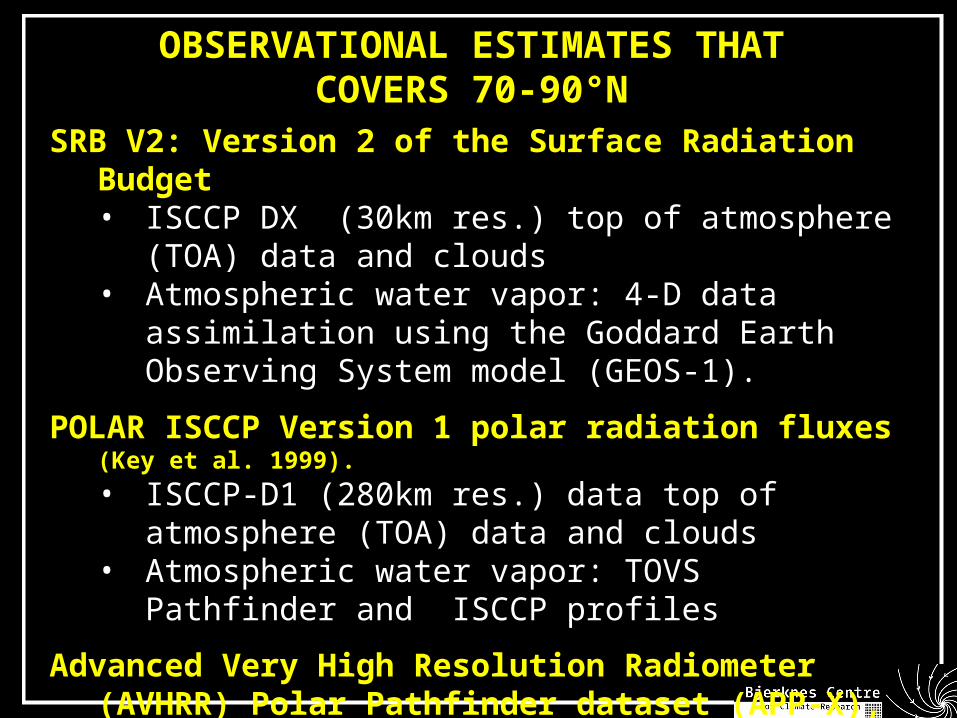
OBSERVATIONAL ESTIMATES THATCOVERS 70-90°N
SRB V2: Version 2 of the Surface Radiation Budget• ISCCP DX (30km res.) top of atmosphere (TOA) data and
clouds• Atmospheric water vapor: 4-D data assimilation using the
Goddard Earth Observing System model (GEOS-1).
POLAR ISCCP Version 1 polar radiation fluxes (Key et al. 1999).
• ISCCP-D1 (280km res.) data top of atmosphere (TOA) data and clouds
• Atmospheric water vapor: TOVS Pathfinder and ISCCP profiles
Advanced Very High Resolution Radiometer (AVHRR) Polar Pathfinder dataset (APP-X), Version 1 (Key, 2001).
• Extension of the standard clear sky products using the Cloud and Surface Parameter Retrieval (CASPR) system
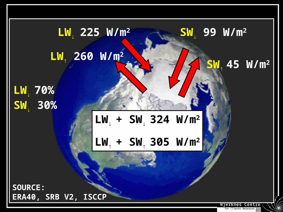
225 W/m2 99 W/m2
260 W/m2
45 W/m2
SW↓LW↓
SW↑
LW↑
LW↓ + SW↓ 324 W/m2
LW↑ + SW↑ 305 W/m2
SOURCE:ERA40, SRB V2, ISCCP
LW↓ 70%SW↓ 30%
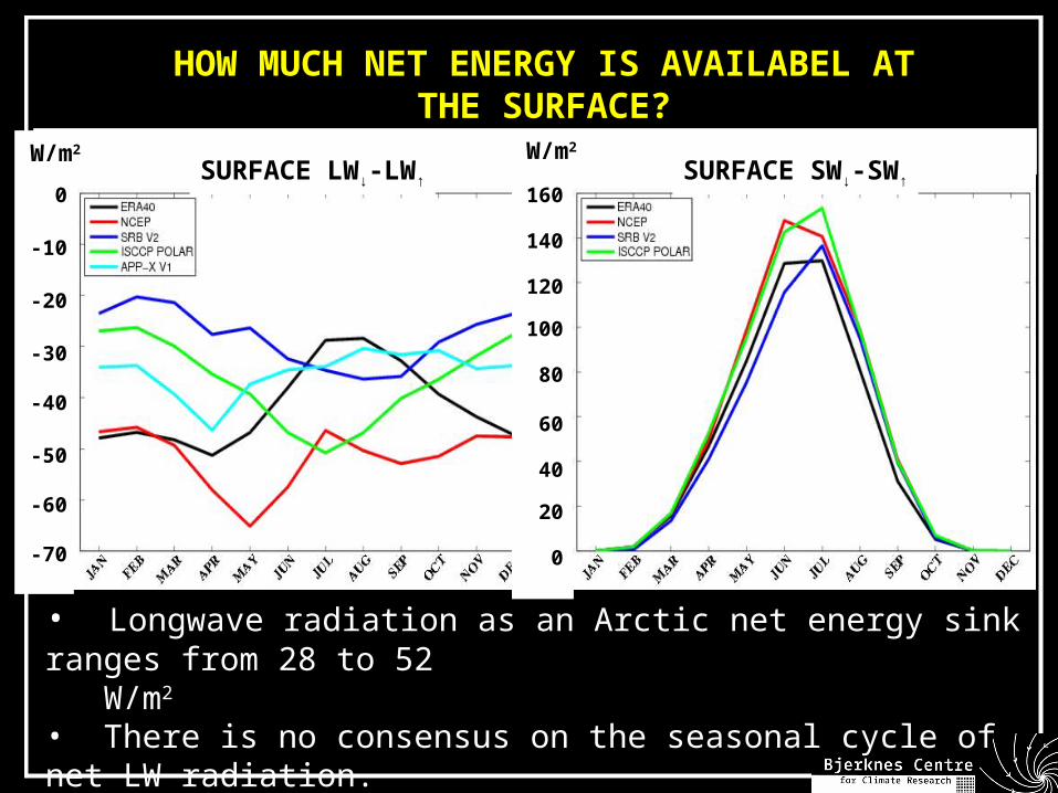
• Longwave radiation as an Arctic net energy sink ranges from 28 to 52 W/m2 • There is no consensus on the seasonal cycle of net LW radiation.• Shortwave radiation as a net energy source ranges from 43 to 50 W/m2
160
140
120
100
80
60
40
20
0
SURFACE LW↓-LW↑ SURFACE SW↓-SW↑
HOW MUCH NET ENERGY IS AVAILABEL AT THE SURFACE?
0
-10
-20
-30
-40
-50
-60
-70
W/m2 W/m2
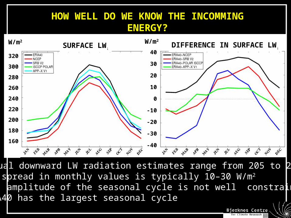
HOW WELL DO WE KNOW THE INCOMMINGENERGY?
• Annual downward LW radiation estimates range from 205 to 230 W/m2 • The spread in monthly values is typically 10–30 W/m2 • The amplitude of the seasonal cycle is not well constrained.• ERA40 has the largest seasonal cycle
265
300
SURFACE LW↓ DIFFERENCE IN SURFACE LW↓
320
300
280
260
240
220
200
180
160
W/m2
40
30
20
10
0
-10
-20
-30
-40
W/m2
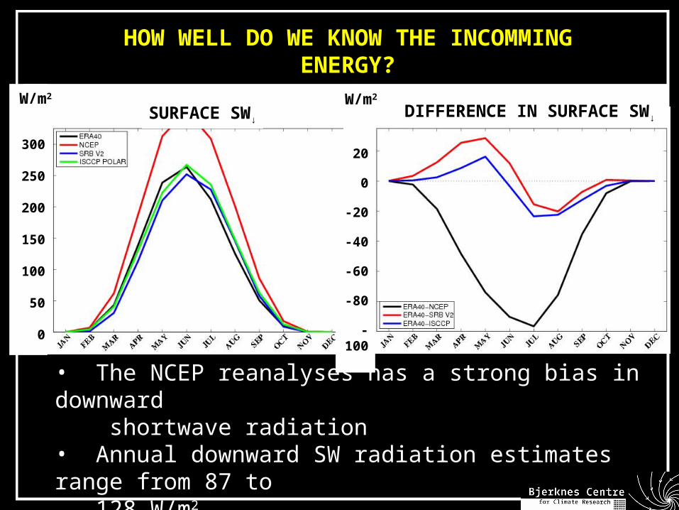
• The NCEP reanalyses has a strong bias in downward shortwave radiation• Annual downward SW radiation estimates range from 87 to 128 W/m2.• The monthly spread is typically 10–20 W/m2 during summer
SURFACE SW↓DIFFERENCE IN SURFACE SW↓
HOW WELL DO WE KNOW THE INCOMMINGENERGY?
300
250
200
150
100
50
0
W/m2
20
0
-20
-40
-60
-80
-100
W/m2
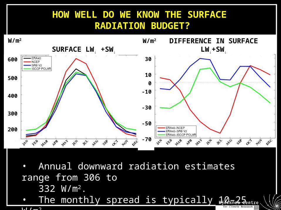
• Annual downward radiation estimates range from 306 to 332 W/m2.• The monthly spread is typically 10–25 W/m2
HOW WELL DO WE KNOW THE SURFACE RADIATION BUDGET?
SURFACE LW↓ +SW↓
DIFFERENCE IN SURFACE LW↓+SW↓
600
500
400
300
200
W/m2
30
10
0
-10
-30
-50
-70
W/m2
HOW WELL IS IT SIMULATED WITHCOUPLED GCMs?
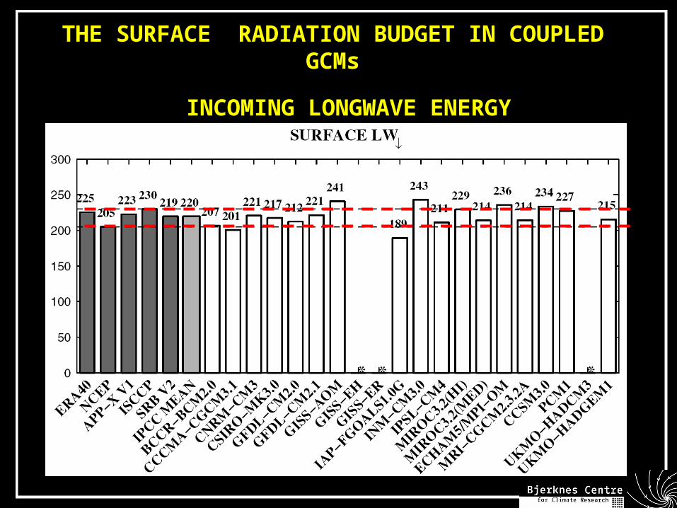
THE SURFACE RADIATION BUDGET IN COUPLED GCMs
INCOMING LONGWAVE ENERGY
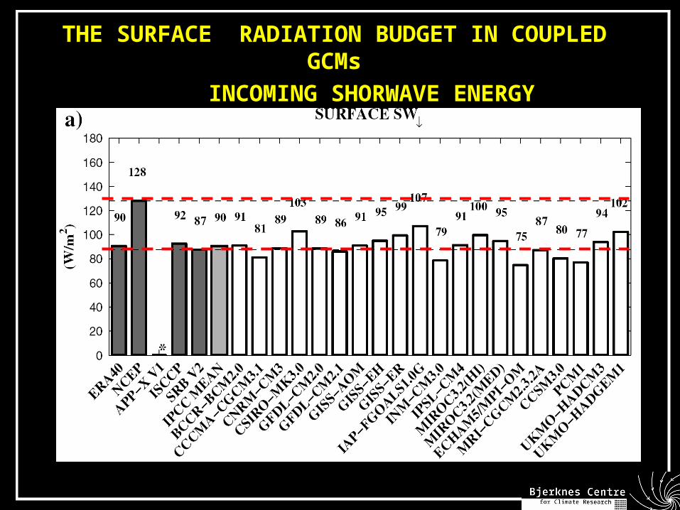
THE SURFACE RADIATION BUDGET IN COUPLED GCMs
INCOMING SHORWAVE ENERGY
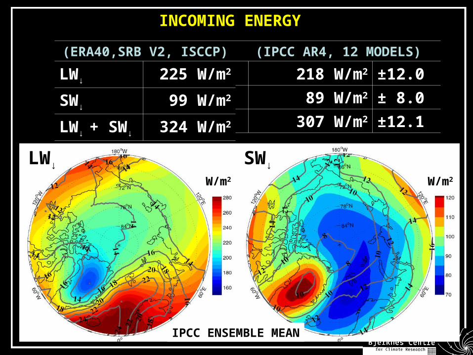
(IPCC AR4, 12 MODELS)
218 W/m2 ±12.0
89 W/m2 ± 8.0
307 W/m2 ±12.1
(ERA40,SRB V2, ISCCP)
LW↓ 225 W/m2
SW↓ 99 W/m2
LW↓ + SW↓ 324 W/m2
INCOMING ENERGY
LW↓ SW↓
W/m2 W/m2
IPCC ENSEMBLE MEAN
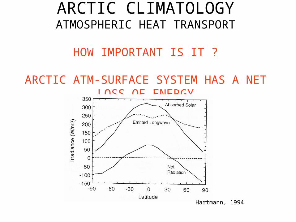
ARCTIC CLIMATOLOGYATMOSPHERIC HEAT TRANSPORT
HOW IMPORTANT IS IT ?
ARCTIC ATM-SURFACE SYSTEM HAS A NET LOSS OF ENERGY
Hartmann, 1994
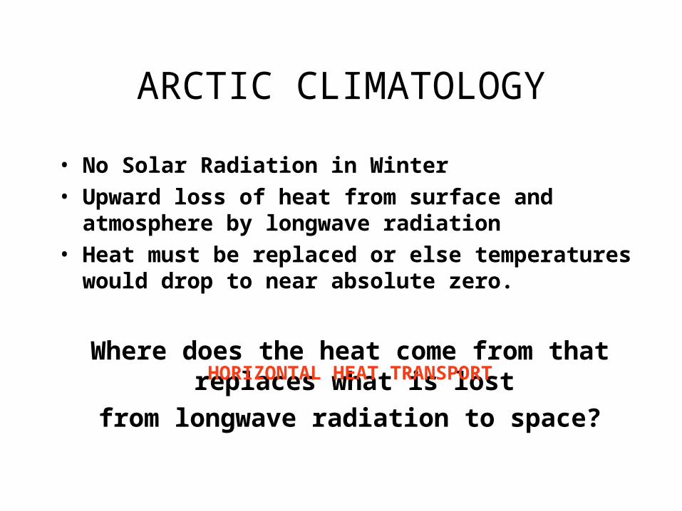
• No Solar Radiation in Winter• Upward loss of heat from surface and atmosphere
by longwave radiation• Heat must be replaced or else temperatures would
drop to near absolute zero.
Where does the heat come from that replaces what is lost
from longwave radiation to space?
HORIZONTAL HEAT TRANSPORT
ARCTIC CLIMATOLOGY
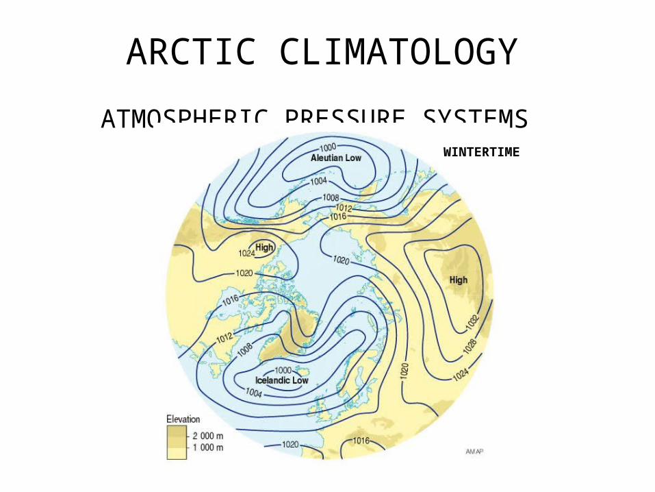
ARCTIC CLIMATOLOGY
ATMOSPHERIC PRESSURE SYSTEMS WINTERTIME