soft x-ray measurement of the thermal electron temperature on the levitated dipole experiment...
TRANSCRIPT

Soft X-ray Measurement of the Thermal Electron Temperature on the Levitated Dipole Experiment (LDX)
M.S. Davis, D.T. Garnier, M.E. MauelColumbia University
J.L. Ellsworth, J. Kesner, P.C. Michael, P. WoskovPSFC MIT

The Levitated Dipole Experiment studies plasma confinement in a magnetic dipole field. Measurement of the plasma pressure profile is of particular interest in determining the whether the dipole geometry is suitable for magnetically confined fusion. Interferometer measurements on LDX have shown the density profile to be “peaked” during levitation but while edge probe temperature measurements and measurements of the hot electron temperature have been made the thermal electron temperature profile has not been determined. Preliminary soft X-ray measurements have approximated a thermal electron temperature of 800 eV. Here we present further soft X-ray measurements made with a Si-PIN diode and pulse height analysis system. By comparing levitated shots with similar supported shots, in which the thermal population is largely absent due to end losses, we deduce the thermal electron temperature. This work is supported by DoE grants: DE-FG02-98ER54458/9.
Abstract

Levitated Dipole Experiment

Levitated Dipole Experiment
Internal super-conducting coil can operate either mechanically supported or magnetically levitated in the chamber.
Plasmas are created using multi-frequency electron cyclotron resonance heating (ECRH).

Hot Electrons up to 60 keV
Measurements of X-rays have been used on LDX to deduce the temperature of the heated, high-energy electron population1.
The temperature of the hot electrons is 20-60 keV.
1 J. L. Ellsworth

Power from Bremsstrahlung as function of frequency and electron temperature
Power from Recombination as function of frequency and electron temperature
Pbrem(!, Te) = NeNiZ2
!e2
4"#o
"3 32"2g
3!
3m2c3
#2m
"Tee!h!Te
" NeNiZ2
#1Te
e!h!Te
Precon(!, Te) = NeNiZ2
!e2
4"#o
"3 32"2g
3!
3m2c3
#2m
"Tee!h!Te
$Z2Ry
Te
2Gn
n3eZ2Ry/n2Te
%
" NeNiZ4
n3T 3/2e
e!h!!|En|
Te

Estimating the TemperatureWe compare probe measurements of the electron temperature at the edge of the LDX plasma to profile models to calculate an estimate of the peak warm electron temperature.
p ! V !! , N ! V !1 " Te ! V !!1
Te(core) ! ? at 0.78 m
Te(edge) ! 25 eV at 1.8 m
N " V !1 " r!4
pV ! = constant
! = 5/3
Te(core)
Te(edge)!
!Vedge
Vcore
"!!1
" (50)!!1 =# Te(core) " 14Te(edge) " 350 eV

ECE Hot Electron Temperature2
2 Paul Woskov
Harmonic ECE measurements suggest that the hot electron temperatures in LDX are broadly in the range of 50 - 150 keV
-higher temperatures at lower densities
These determinations are as yet still uncertain
-Uncertainty of the flux loop location of hot electron density peak (as shown in plot to right)-Temperature assignment implies a Maxwellian distribution-Measurements at additional ECE frequencies could result in different determinations
Determined from 110 and 137 GHz Measurements of Harmonic Emission

Si (PIN) Diode Detector
Detector features• 1 - 20 keV range• 0.5 mil Be window • Reset preamplifier• Reset time 1 μs• Peltier cooler
Fe55 Peak (multiple low pile up spectra)
0 2 4 6 8 10 12Energy (keV)
0
1000
2000
3000
4000
5000
Counts
<---- FWHM = 336 eV---->
|---- 5.9 keV
|---- 6.5 keV
Detector used was the XR-100Cr made by Amptek
How the detector works:An X-ray photon is absorbed in the detector principally via the photoelectric effect freeing electrons. The detector is biased so these free charges accumulate across a capacitor creating a voltage that can be measured. The size of the voltage increase across the capacitor is proportional to the photon energy.
Detector Transmission/Absorption
0 5 10 15 20 25Energy (keV)
0.0
0.2
0.4
0.6
0.8
1.0
Tran
smiss
ion
<- low energies blocked by 0.5 mil Be window
high energies passthru 300 micron silicon
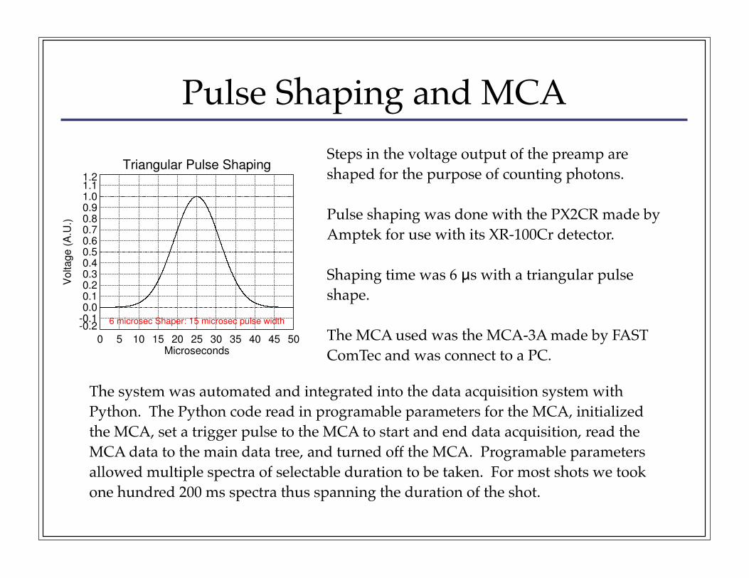
Pulse Shaping and MCASteps in the voltage output of the preamp are shaped for the purpose of counting photons.
Pulse shaping was done with the PX2CR made by Amptek for use with its XR-100Cr detector.
Shaping time was 6 μs with a triangular pulse shape.
The MCA used was the MCA-3A made by FAST ComTec and was connect to a PC.
The system was automated and integrated into the data acquisition system with Python. The Python code read in programable parameters for the MCA, initialized the MCA, set a trigger pulse to the MCA to start and end data acquisition, read the MCA data to the main data tree, and turned off the MCA. Programable parameters allowed multiple spectra of selectable duration to be taken. For most shots we took one hundred 200 ms spectra thus spanning the duration of the shot.
Triangular Pulse Shaping
0 5 10 15 20 25 30 35 40 45 50Microseconds
-0.2-0.10.00.10.20.30.40.50.60.70.80.91.01.11.2
Volta
ge (A
.U.)
6 microsec Shaper: 15 microsec pulse width

Pile-upCounts and Deadtime with Distance
2 4 6 8 10 12 14Distance to Source (cm)
0
2
4
6
8
10
Co
un
t R
ate
(kC
ps)
Spectra at 15.0 cm
0 1000 2000 3000 4000 5000 6000Bin
0
200
400
600
Co
un
ts
Deadtime: 5.695 %
Spectra at 10.0 cm
0 1000 2000 3000 4000 5000 6000Bin
0200
400
600
800
10001200
Co
un
ts
Deadtime: 12.140 %
Spectra at 5.0 cm
0 1000 2000 3000 4000 5000 6000Bin
0
500
1000
1500
Co
un
ts
Deadtime: 28.115 %
Spectra at 2.0 cm
0 1000 2000 3000 4000 5000 6000Bin
0
100
200
300
400
500
Co
un
ts
Deadtime: 44.565 %
Spectra at 0.5 cm
0 1000 2000 3000 4000 5000 6000Bin
0
5
10
15
20
25
Co
un
ts Deadtime: 40.190 %
0
10
20
30
40
50
De
ad
Tim
e (
%)
Pile-up occurs when two X-ray photons hit the detector nearly simultaneously. The pulse counting system can only count one pulse at a time so pile-up can distort the spectrum. Algorithms are used to try to identify times when pile-up is occurring and omit counts during those times from the spectrum. Thus if pile-up is too high the count rate will go down.
Pile-up rejection algorithms were implemented in both the shaping amplifier and in the MCA.
The 6 μs shaping time of the shaper put a severe limit on the maximum count rate.
By varying the distance of an Fe55 source we found max count rate of the system to be 9 kCps.
Note that the deadtime listed at left only reflects deadtime measured by MCA, not deadtime measured by the shaping amplifier.

Detector CalibrationsFe55 Spectrum: Gain 1
0 20 40 60 80Energy (keV)
0
2000
4000
6000
8000
10000
Co
un
ts
Fe55 Spectrum: Gain 2
0 10 20 30 40Energy (keV)
0
1000
2000
3000
4000
5000
Co
un
ts
Fe55 Spectrum: Gain 4
0 5 10 15 20Energy (keV)
0
500
1000
1500
2000
2500
Co
un
ts
Am241 Spectrum: Gain 1
0 20 40 60 80Energy (keV)
0
500
1000
1500
2000
2500
Co
un
ts
Am241 Spectrum: Gain 2
0 10 20 30 40Energy (keV)
0
200
400
600
800
1000
1200
Co
un
ts
Am241 Spectrum: Gain 4
0 5 10 15 20Energy (keV)
0
200
400
600
800
1000
1200
Co
un
ts
Detector Calibration
1000 2000 3000 4000 5000 6000Bin
0
20
40
60
Energ
y (
keV
)
y = (0.01537) x + (0.18876)
y = (0.00771) x + (-0.03719)
y = (0.00392) x + (-0.03127)
Gain = 1
Gain = 2
Gain = 4
The detector and MCA system were calibrated using and Fe55 source and an Am241 source

Experimental Setup
Experiment Transmission/Absorption
0 5 10 15 20 25Energy (keV)
0.0
0.2
0.4
0.6
0.8
1.0
Tran
smiss
ion
<--- low energies blocked by 0.5 mil Be window, 2.0 mil Be Window, and 2 cm air
high energies passthru 300 micron silicon
Vacuum/PlasmaAir
2 mil Be WindowDetector
Pinhole
Holder
0.5 mil Be Window
Lead
Pinholes
Vacuum chamber5 meters
Floating Coil115 cm diameter
Port with pinhole and filtersDetector
The detector viewed the plasma through a 2 mil Be port window, 2 cm of air and a 0.5 mil Be window built on the detector. The view was in the equatorial plane with a tangent radius between 80 and 90 cm.

Observations of Pile-up
Combined Spectrum: Shot 90722010
0 2 4 6 8 10Energy (keV)
0
20
40
60
80
Coun
ts Gain 4.00Pinhole 0.05
0.0
1.7
3.3
5.0
0 5 10 15Time (sec)
0
2
4
6
8
Ener
gy (k
eV)
Time Spectra: Shot 90722010
Count Rate
0 5 10 15Time (sec)
0.0
0.5
1.0
1.5
2.0
Rate
(kCp
s)ECRH
0 5 10 15Time (sec)
0
2
4
6
8
10
12
Interferometer
0 5 10 15Time (sec)
0
2
4
6
8
10
Combined Spectrum: Shot 90723014
0 2 4 6 8 10Energy (keV)
0
200
400
600
800
Coun
ts Gain 1.00Pinhole 0.14
0.0
13.
26.
39.
0 5 10 15Time (sec)
2
4
6
8
Ener
gy (k
eV)
Time Spectra: Shot 90723014
Count Rate
0 5 10 15Time (sec)
0
1
2
3
4
5
Rate
(kCp
s)
ECRH
0 5 10 15Time (sec)
0
2
4
6
8
10
12
Interferometer
0 5 10 15Time (sec)
02
4
6
8
10
1214
Much Pile-up Little Pile-up

Levitated vs. SupportShot: 90724016
0 5 10 15 20Energy (keV)
1
2
3
4
5
6
Inte
nsity
(A.U
.)
Shot: 90722010
0 5 10 15 20Energy (keV)
1
2
3
4
5
6
Inte
nsity
(A.U
.)
Levitated shots consistently exhibited a peaking up in the spectrum at lower energies that was not seen in the support shots. This may be due to a thermal population that is not present in the supported cases.
Note that due to the small number of support shots taken and the large number of levitated shots that were dominated by pile-up there were no shots to compare where levitation was the only varied parameter (i.e., heating in these two shots is not identical).

Levitated Shot: 90722010
Spectrum Time=[0.0 , 19.8]
0 2 4 6 8 10Energy (keV)
0
20
40
60
80
Coun
ts
0.0
0.2
0.4
0.6
0.8
1.0
Tran
smiss
ion
Shot: 90722010
0 5 10 15 20Energy (keV)
0
100
200
300
Inte
nsity
Shot: 90722010
0 5 10 15 20Energy (keV)
1
2
3
4
5
6
Inte
nsity
(A.U
.)
Double Maxwellian FitTe = 23.6 keVTe = 0.323 keV
0.0
1.7
3.3
5.0
0 5 10 15Time (sec)
0
5
10
15
Ener
gy (k
eV)
Shot: 90722010
Fitting the levitated data to a double Maxwellian distribution gives a warm temperature of 300 eV and a hot temperature of 23 keV.
Corrections for transmission do not account for the lack of counts at 2-4 keV (in first panel the red diamonds are the transmission corrected counts).
In panels 2 and 3 the red diamonds indicate the peaking in the spectrum that is observed in levitated shots but not in supported shots.

Supported Shot: 90724013
Spectrum Time=[0.0 , 19.8]
0 2 4 6 8 10Energy (keV)
0
10
20
30
40
50
Coun
ts
0.0
0.2
0.4
0.6
0.8
1.0
Tran
smiss
ion
Shot: 90724013
0 5 10 15 20Energy (keV)
0
20
40
60
80
Inte
nsity
Shot: 90724013
0 5 10 15 20Energy (keV)
1
2
3
4
5
6
Inte
nsity
(A.U
.) Te = 10.2 keV
0.0
1.3
2.7
4.0
0 5 10 15Time (sec)
0
5
10
15
Ener
gy (k
eV)
Shot: 90724013
Fitting the data to a single Maxwellian distribution gives a temperature of 10 keV.
The red diamonds in panel 1 show the counts corrected for transmission. The corrected counts match the exponential spectrum seen at higher energies.
The red diamond in panels 2 and 3 show the bins where the spectrum peaks in levitated shots.

AfterglowCombined Spectrum: Shot 90724040
0 2 4 6 8 10Energy (keV)
0
100
200
300
400
500
600
Coun
ts Gain 1.00Pinhole 0.14
0.0
12.
23.
35.
0 5 10 15Time (sec)
2
4
6
8
Ener
gy (k
eV)
Time Spectra: Shot 90724040
Count Rate
0 5 10 15Time (sec)
0
1
2
3
4
5
Rate
(kCp
s)
ECRH
0 5 10 15Time (sec)
0
1
2
3
Interferometer
0 5 10 15Time (sec)
0
1
2
3
4
Pile-up made most spectra taken during the heating phases distorted and difficult to interpret. This was particularly true in the helium and argon shots. The plot to the left is an argon shot.
The middle panel shows the count rate rise early in the shot then decrease during the shot due to pile-up and rise at the end of the shot when the heating sources have been turned off. Panel 2 shows the spectral structure varying with the count rate.
The count rate during the afterglow (the period after the heating sources have been turned off, 14-20 seconds) dropped and there was less pile-up. Thus we are able to examine the spectra during the afterglow of the helium and argon shots.

Afterglow: Helium and ArgonHe Afterglow (second 15 onward) Spectrum
0 2 4 6 8 10Energy (keV)
0
100
200
300
400
500
600
Coun
ts
-Counts
-Fit
Ar Afterglow (second 15 onward) Spectrum
0 2 4 6 8 10Energy (keV)
0
100
200
300
Coun
ts
-Counts
-Fit
For the levitated helium and argon shots pile-up was high for the entire shot except during the afterglow.
Just as in the levitated D2 shots a peak at about 4.5 keV is observed in both the helium and argon afterglow. This may be a titanium line or counts from a warm thermal population, although there is a dearth of counts below it.
The peak in the argon afterglow at 3 keV corresponds to several K shell transitions in argon. The presence of this peak in the argon afterglow shows the detector was sensitive to counts in that range and suggests that the feature at 4.5 keV may be a peak.

Silicon Drift Detector
Detector features:• 190 eV FWHM Resolution at 5.9 keV with 0.8 μs peaking time• 500 kCps• Thermoeletrically cooled• 1 mV/keV preamp sensitivity• Reset preamp
The Silicon Drift Detector (SDD) has a much lower capacitance than an Si(PIN) diode of comparable size thus reducing the electrical noise and allowing it to maintain good performance at short shaping times and high count rates.

Digital MCA
For the next experiment run we are going to run the preamp output to a fast digitizer (50 MSPS). The board is built by D-tAcq and can record 4 channels at 50 MSPS or more channels at lower sample rate.
Digitizing the preamp output will give us the information to design a shaping-counting system with optimal parameters (shaping time, pile-up rejection, etc.) and give us greater confidence in our spectra.
Further, the four channels allow for other existing PHA systems to be similarly improved. Specifically, we will be able to look at the higher energy spectra with an NaI detector and a CZT detector. The performance of the Si(PIN) with shorter shaping times could also be explored.

CZT and NaI Detectors1
NaI
CZT
CZT (Cadmium Zinc Telluride)• Energy range: 10 - 670 keV• Energy resolution: 4% FWHM at 122 keV• Nominal sensitivity: 0.11 mV/keV• Rise time at the source: 35 ns• RC decay time: 750 μs
1 J. L. Ellsworth
NaI (Sodium Iodide)• Energy range: 10 keV - 2 MeV• Output measures total X-ray intensity from the plasma

Radial Ambitions
Vacuum chamber
5 meters
Floating Coil
115 cm diameter
Port with pinhole and filtersLinear array of SDDs
Parameters at SDD array location:
Magnetic field: 10 G (during experiment)
500 G (while charging floating coil)
Temperature: 293 K (room temperature)
Vacuum: 1e-8 Torr
LDX SDD Array : Basic Layout Sketch Ultimately we want radial measurements of the temperature so we can construct a radial temperature profile. With the radial temperature profile and the radial density profile (obtained from the interferometer) we will be able to determine the adiabatic index in LDX.
We are exploring two designs: the first simply involves using more SDDs while the second uses an X-ray camera with a diffractive medium. In the latter, one axis of the camera records spectral information while the other records radial information. The latter would provide far more chord views allowing for better a radial reconstruction but is more likely to encounter signal to noise problems.

Conclusion
We present preliminary measurements of the low energy (2 - 20 keV) X-ray spectrum on LDX. The measurements were made with an Si(PIN) diode detector. We encountered a considerable amount of pile-up in our measurements that made the spectra complicated to interpret. Our principal observation is that there is a distinct difference between spectra in levitated and supported shots: levitated spectra are significantly peaked at lower energies while support spectra are not. Modeling the plasma as a double Maxwellian distribution we measure the warm electron temperature to be 300 eV. Determining whether this peaking is due to bremsstrahlung from a warm thermal electron population or some other spectral feature is important. To determine this we are building an SDD system that will be able to handle much higher count rates and allow us to see to lower energies. Once we obtain good single chord spectra we will build a multi-chord instrument in order to get a radial profile of the soft X-ray emission.