single-channel speech separation based on …
TRANSCRIPT

SINGLE-CHANNEL SPEECH SEPARATION BASED ON INSTANTANEOUSFREQUENCY
By
LINGYUN GU
Thesis Committee:Richard M. Stern, Chair (Carnegie Mellon University)
Bhiksha Raj (Carnegie Mellon University)Alex Rudnicky (Carnegie Mellon University)
Dan Ellis (Columbia University)
A DISSERTATION PRESENTED TO THE GRADUATE SCHOOLOF CARNEGIE MELLON UNIVERSITY IN PARTIAL FULFILLMENT
OF THE REQUIREMENTS FOR THE DEGREE OFDOCTOR OF PHILOSOPHY
CARNEGIE MELLON UNIVERSITY
2010

c© 2010 Lingyun Gu
To my beloved wife, Jing
To my parents
To my baby girl, Yiya
To all Bodhisattvas who have been blessing and shining my family

ACKNOWLEDGMENTS
My dissertation comes from two parts. One is necessary. But the other is essential. The
former is my diligent though nature-decide-limited effort. The latter is a tremendous and
unbounded amount of love and help I have been receiving from many people whom I want
to thank here.
No doubt I want to bring my advisor Richard Stern to the first place to thank him for his
immense support, guidance, help and fruitful discussions over the past six years. He brought
me to Carnegie Mellon to help me fulfill my dream to get professional training not only at a
top school, but also in one of the world-class labs in the speech recognition area. What he
says and does sets up a perfect model for me to follow, not only in the area of research, but
also extended to many other fields. There is an old Chinese saying, ”One day your advisor,
forever your father”. I want to borrow this adage and give my endless gratitude to him, for
everything he does for me.
I also want to take this opportunity to thank my thesis committee members, Professors
Bhiksha Raj, Alex Rudnicky and Dan Ellis, for their valuable suggestions, comments and
great ideas. Special thanks also goes to Bhiksha, for his role not only being my committee
member, but also a truly helpful elder academic brother.
Members of the almighty robust speech recognition group also have played a very important
role in both my research and dissertation writing. Many thanks to previous members Alex
Acero, Evandro Gouea, Pedro Moreno, Xiang Li and current members Rita Singh, Kshitiz
Kumar, Ziad Al Bawab, Chanwoo Kim and Yuhsiang Chiu, for their abundant discussions.
My best friends cross the country also deserve an equal amount of my gratitude. Jun Qian,
Rui Yan, Wei Ye, Wei Luo, Jingdong Deng, Hailing Wang, Gao Yao, Qi Xiangli, Zhipan
Guo, Jinge Zhong, Shuguang Tan, Henry Lin, Grace Yang, Kamin Chang, Jin Xie, Rong
Zhang, Ying Zhang, Rong Yan, Yan Liu, Wen Wu, Yanjun Qi, Le Zhao, Ni Lao, Luo Si, Hua
Yu, Chun Jin, Jian Zhang, Yue Cui, Pradipta Ray, Andrew Schlaikjer, Hideki Shima, Oznur
i

Tastan, Andres Zollmann, Matthew Bilotti, Meryem Donmez, Yiqing Wang, Hang Yu and
Justin Betteridge, thank all of you for your endless support.
I am truly grateful to my parents. I couldn’t have achieved anything without their
enormous time, energy, love since the first moment I came to this world. Even though they
are living thousands miles away from me in China, their love breezes me everyday and will
continue forever.
The last, but never ever the least indebtedness, goes to my beloved wife Jing. Without her
years of years continuous support, my dissertation could not possibly have been completed.
Neither Shakespeare nor Dickens can come up with the best words I can ever use to tell her
how fortunate I am to share happiness and shred tears with her together. She is the fifth
element in my life.
ii
TABLE OF CONTENTS
page
ACKNOWLEDGMENTS . . . . . . . . . . . . . . . . . . . . . . . . . . . . . . . . . i
LIST OF TABLES . . . . . . . . . . . . . . . . . . . . . . . . . . . . . . . . . . . . . vi
LIST OF FIGURES . . . . . . . . . . . . . . . . . . . . . . . . . . . . . . . . . . . . vii
ABSTRACT . . . . . . . . . . . . . . . . . . . . . . . . . . . . . . . . . . . . . . . . x
CHAPTER
1 INTRODUCTION . . . . . . . . . . . . . . . . . . . . . . . . . . . . . . . . . . 1
1.1 Motivation . . . . . . . . . . . . . . . . . . . . . . . . . . . . . . . . . . . . 11.1.1 Speech Separation Systems . . . . . . . . . . . . . . . . . . . . . . . 21.1.2 Why is Single-Channel Speech Recognition Important? . . . . . . . 31.1.3 Why is Single-Channel Speech Recognition Challenging? . . . . . . 4
1.2 Overview of the Speech Separation System base on Instantaneous Frequency 41.3 Dissertation Outline . . . . . . . . . . . . . . . . . . . . . . . . . . . . . . 5
2 REVIEW OF ALGORITHMS FOR SINGLE-CHANNEL SPEECH SEPARATION 7
2.1 CASA Introduction . . . . . . . . . . . . . . . . . . . . . . . . . . . . . . . 72.1.1 Motivation for Exploiting CASA . . . . . . . . . . . . . . . . . . . . 82.1.2 Examples of CASA Systems and Applications . . . . . . . . . . . . 102.1.3 CASA Mask Generation and Evaluation . . . . . . . . . . . . . . . . 11
2.2 Amplitude-Modulation Spectral Analysis . . . . . . . . . . . . . . . . . . . 122.2.1 Amplitude Modulation based Algorithms . . . . . . . . . . . . . . . 132.2.2 Differences between Amplitude and Frequency Modulation Schemes 15
2.3 Multi-Pitch Tracking based Speech Separation . . . . . . . . . . . . . . . . 16
3 ESTIMATION OF INSTANTANEOUS FREQUENCY AND ITS APPLICATIONTO SOURCE SEPARATION . . . . . . . . . . . . . . . . . . . . . . . . . . . . 19
3.1 Modulation Frequency and Its application to Speech Separation . . . . . . 193.2 Instantaneous Frequency and Its Calculation . . . . . . . . . . . . . . . . . 22
3.2.1 Instantaneous Frequency Calculation . . . . . . . . . . . . . . . . . 223.2.2 Two Alternative ways to Calculate Instantaneous Frequency . . . . 28
3.3 Instantaneous Frequency Estimation for Frequency-modulated Complex Tone 313.3.1 Frequency-modulated Complex Tones . . . . . . . . . . . . . . . . . 323.3.2 Extracting Instantaneous Frequency from Frequency-modulated
Complex Tones . . . . . . . . . . . . . . . . . . . . . . . . . . . . . 333.4 Factors Affecting Instantaneous Frequency Estimation . . . . . . . . . . . 35
iii

4 CROSS-CHANNEL CORRELATION AND OTHER MASK-CLUSTERINGMETHODS . . . . . . . . . . . . . . . . . . . . . . . . . . . . . . . . . . . . . . 38
4.1 Cross-channel Correlation . . . . . . . . . . . . . . . . . . . . . . . . . . . 384.1.1 Patterns of Separated Speech Components Obtained by Cross-channel
Correlation . . . . . . . . . . . . . . . . . . . . . . . . . . . . . . . . 394.1.2 Mean Square Difference Mask Generation . . . . . . . . . . . . . . . 44
4.2 One-Dimensional Projection Solution . . . . . . . . . . . . . . . . . . . . . 474.3 Graph-Cut Solution . . . . . . . . . . . . . . . . . . . . . . . . . . . . . . . 50
5 GROUPING SCHEMES AND EXPERIMENTAL DESIGN . . . . . . . . . . . 57
5.1 Grouping Schemes . . . . . . . . . . . . . . . . . . . . . . . . . . . . . . . 575.1.1 Pitch Detection for Dominant Speakers for the Different-Gender Case 585.1.2 Speaker Identification for the Same-Gender Case . . . . . . . . . . . 59
5.2 Mask Generation . . . . . . . . . . . . . . . . . . . . . . . . . . . . . . . . 615.3 Experimental Procedures and Databases . . . . . . . . . . . . . . . . . . . 63
5.3.1 Sphinx-III Recognition Platform . . . . . . . . . . . . . . . . . . . . 635.3.2 The Resource Management and Grid Corpora . . . . . . . . . . . . 63
5.4 Experimental Results and Discussion . . . . . . . . . . . . . . . . . . . . . 665.5 A Sieve Function for Selecting Relevant Frequency Components from Partial
Harmonic Structure . . . . . . . . . . . . . . . . . . . . . . . . . . . . . . . 715.5.1 Harmonic Pattern Recognition . . . . . . . . . . . . . . . . . . . . . 715.5.2 The Harmonic Sieve . . . . . . . . . . . . . . . . . . . . . . . . . . . 735.5.3 Objective Function . . . . . . . . . . . . . . . . . . . . . . . . . . . 74
6 INSTANTANEOUS-AMPLITUDE-BASED SEGREGATION FOR UNVOICEDSEGMENTS . . . . . . . . . . . . . . . . . . . . . . . . . . . . . . . . . . . . . 77
6.1 Feature Extraction Based on Instantaneous Amplitude . . . . . . . . . . . 786.2 Detection of Boundaries Between Voiced and Unvoiced Segments . . . . . . 80
6.2.1 The Teager Energy Operator . . . . . . . . . . . . . . . . . . . . . . 826.2.2 Autocorrelation . . . . . . . . . . . . . . . . . . . . . . . . . . . . . 826.2.3 Energy Detection . . . . . . . . . . . . . . . . . . . . . . . . . . . . 836.2.4 Zero Crossing Rate (ZCR) . . . . . . . . . . . . . . . . . . . . . . . 836.2.5 Ratio of Energy in High and Low Frequency Bands . . . . . . . . . 85
6.3 Experimental Results using Instantaneous Amplitude-based Segregation . . 866.3.1 Evaluation of V/UV Decisions . . . . . . . . . . . . . . . . . . . . . 866.3.2 Evaluation of WER Using Amplitude-Based Features . . . . . . . . 87
7 SUMMARY AND CONCLUSIONS . . . . . . . . . . . . . . . . . . . . . . . . . 89
7.1 Major Findings and Contributions . . . . . . . . . . . . . . . . . . . . . . . 897.2 Directions of Possible Future Research . . . . . . . . . . . . . . . . . . . . 90
7.2.1 Combine long term and short term cross-channel correlation . . . . 907.2.2 Combine instantaneous frequency and amplitude . . . . . . . . . . . 907.2.3 Introduce image processing algorithms for mask generation . . . . . 90
iv
7.3 Summary and Conclusions . . . . . . . . . . . . . . . . . . . . . . . . . . . 91
REFERENCES . . . . . . . . . . . . . . . . . . . . . . . . . . . . . . . . . . . . . . . 92
BIOGRAPHICAL SKETCH . . . . . . . . . . . . . . . . . . . . . . . . . . . . . . . . 96
v
LIST OF TABLES
Table page
3-1 Correlation comparison among harmonic members and between harmonic andnon-harmonic members. . . . . . . . . . . . . . . . . . . . . . . . . . . . . . . . 36
4-1 Correlation using the cross-channel correlation method. . . . . . . . . . . . . . . 46
4-2 Instantaneous frequency distance using the mean square difference method. . . . 47
4-3 Confusion matrix of performance of selected harmonic frequencies for the cleancase using the 1-D projection method. . . . . . . . . . . . . . . . . . . . . . . . 49
4-4 Confusion matrix of performance of selected harmonic frequencies at 15 dB usingthe 1-D projection method. . . . . . . . . . . . . . . . . . . . . . . . . . . . . . 49
4-5 Confusion matrix of performance of selected harmonic frequencies at 10 dB usingthe 1-D projection method. . . . . . . . . . . . . . . . . . . . . . . . . . . . . . 50
4-6 Confusion matrix of performance of selected harmonic frequencies at 5 dB usingthe 1-D projection method. . . . . . . . . . . . . . . . . . . . . . . . . . . . . . 50
4-7 Confusion matrix of performance of selected harmonic frequencies at 0 dB usingthe 1-D projection method. . . . . . . . . . . . . . . . . . . . . . . . . . . . . . 50
4-8 Confusion matrix of performance of selected harmonic frequencies for the cleancase by using the graph-cut method. . . . . . . . . . . . . . . . . . . . . . . . . 53
4-9 Confusion matrix of performance of selected harmonic frequencies at 15 dB byusing the graph-cut method. . . . . . . . . . . . . . . . . . . . . . . . . . . . . . 53
4-10 Confusion matrix of performance of selected harmonic frequencies at 10 dB byusing the graph-cut method. . . . . . . . . . . . . . . . . . . . . . . . . . . . . . 54
4-11 Confusion matrix of performance of selected harmonic frequencies at 5 dB byusing graph-cut method. . . . . . . . . . . . . . . . . . . . . . . . . . . . . . . . 54
4-12 Confusion matrix of performance of selected harmonic frequencies at 0 dB byusing graph-cut method. . . . . . . . . . . . . . . . . . . . . . . . . . . . . . . . 54
5-1 Structure of the sentences in the Grid database. . . . . . . . . . . . . . . . . . . 65
6-1 Confusion matrix of voiced and unvoiced detection using pitch detectiondeveloped by de Cheveigne. . . . . . . . . . . . . . . . . . . . . . . . . . . . . . 86
6-2 Confusion matrix of voiced and unvoiced detection using features developed inthis thesis. . . . . . . . . . . . . . . . . . . . . . . . . . . . . . . . . . . . . . . . 88
vi

LIST OF FIGURES
Figure page
2-1 A simplified end-to-end CASA speech separation system, where the most threeimportant parts are domain transformation, speech-component segregation, andspeech-component regrouping. . . . . . . . . . . . . . . . . . . . . . . . . . . . . 9
2-2 In CASA, speech can be first projected into time-frequency cells in a 2-Drepresentation. Based on how close each time-frequency region is relative to theothers, the regions can be grouped and reconstructed into streams from differentsources. How to classify each region and use various cues to group them intostreams provides great flexibility to reconstruct target speech from interferingsources. . . . . . . . . . . . . . . . . . . . . . . . . . . . . . . . . . . . . . . . . 10
2-3 The speech signal is first decomposed into a time-frequency representation bySTFT. Then within each frequency channel, a second FFT is calculated to transferto time-frequency representation to a frequency-frequency representation, whereone frequency axis represents physical frequency and the other frequency axisrepresents modulation frequency. . . . . . . . . . . . . . . . . . . . . . . . . . . 14
2-4 In this figure, panel (a) shows a pure tone with period T. The correspondingspectra peak is also shown on the right. Panels (b), (c), (d) and (e) share thesame period T of the signal in panel (a) with different waveforms. However, bylooking at the spectral response on the right, it is truly difficult to determine thefundamental frequency simply by locating the position of the global spectra peak. 17
2-5 A mixture of speech and interference is processed in four main stages afterthe cochlear filtering. First, a normalized correlogram is obtained within eachchannel. Channel/peak selection is performed to select a subset of relativelyclean frequency channels. In this third stage, the periodicity information isintegrated across neighborhood channels. Finally, an HMM is utilized to formcontinuous pitch tracks. . . . . . . . . . . . . . . . . . . . . . . . . . . . . . . . 18
3-1 Spectrogram of a chirp signal whose frequency increases linearly with time. . . . 20
3-2 A simple example compares the concepts of modulation frequency, deviationfrequency, and instantaneous frequency. In the figure, the modulation frequencyis 5 Hz, the deviation frequency is 20 Hz. The modulation period is 200 ms, thereciprocal of the modulation frequency of 5 Hz. . . . . . . . . . . . . . . . . . . 21
3-3 A block diagram that describes how instantaneous frequency is calculated by themethod discussed in Equation 3.6. . . . . . . . . . . . . . . . . . . . . . . . . . . 25
3-4 A block diagram that describes how instantaneous frequency is calculated byusing the method discussed in Equation 3.15. . . . . . . . . . . . . . . . . . . . 26
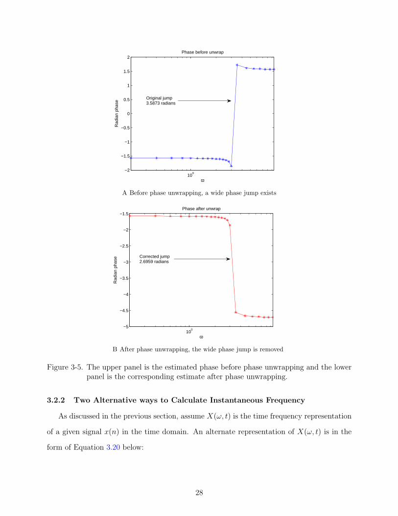
3-5 The upper panel is the estimated phase before phase unwrapping and the lowerpanel is the corresponding estimate after phase unwrapping. . . . . . . . . . . . 28
vii

3-6 The instantaneous frequency estimate of a multi-sinusoid signal using Equations3.6 or 3.15. . . . . . . . . . . . . . . . . . . . . . . . . . . . . . . . . . . . . . . 29
3-7 A general diagram of how instantaneous frequency is calculated by using thedifferentiated window method discussed in Equation 3.29. . . . . . . . . . . . . . 32
3-8 The instantaneous frequency estimation from a multi-sinusoid signal usingcontinuous window derivative methods. . . . . . . . . . . . . . . . . . . . . . . . 33
3-9 Spectrogram of the sum of three frequency-modulated complex tones. . . . . . . 34
3-10 Instantaneous frequencies estimated from corresponding frequency channels froma frequency-modulated complex tones at SNR 0 dB, where the upper and middlesignal are from the same harmonic structure and the lower signal is from anotherirrelevant channel. . . . . . . . . . . . . . . . . . . . . . . . . . . . . . . . . . . 35
4-1 Instantaneous frequency estimates from corresponding frequency channels wherea multi-sinusoid target signal and the single-sinusoid interfering signal have mostof their energy. . . . . . . . . . . . . . . . . . . . . . . . . . . . . . . . . . . . . 41
4-2 Spectrogram of the signal described in Equation 4.3. . . . . . . . . . . . . . . . 42
4-3 Cross-channel correlation of four frequency channels where a multi-sinusoidtarget signal and single-sinusoid interfering signal have most of their energy. . . 43
4-4 Cross-channel correlation of a typical frequency-modulated complex tone at thefundamental frequency of 150 Hz. . . . . . . . . . . . . . . . . . . . . . . . . . . 44
4-5 Cross-channel correlation over all frequency bins for a short voiced segment withfundamental frequency 135.5 Hz. The red and yellow regions represent highcorrelation, while blue and green regions represent low correlation. . . . . . . . . 45
4-6 One-dimensional projection for the same signal used in Figure 4-2. . . . . . . . . 48
4-7 An undirected graph G, which has 9 vertices and should be divided into twopartitions. . . . . . . . . . . . . . . . . . . . . . . . . . . . . . . . . . . . . . . . 52
4-8 Graph-cut method to extract classification information from correlation matrix. 55
4-9 1-D projection method to extract classification information from correlation matrix. 56
5-1 Block diagram of a system that uses pitch detection to determine the dominantspeaker. . . . . . . . . . . . . . . . . . . . . . . . . . . . . . . . . . . . . . . . . 60
5-2 Block diagram of a speech separation system that uses speaker identification todetermine the dominant speaker. . . . . . . . . . . . . . . . . . . . . . . . . . . 62
5-3 A block diagram of the Sphinx-III speech recognition system. . . . . . . . . . . 64
viii

5-4 Experimental results using the RM database that compare the performance of thegraph-cut and 1-D projection methods. The two speakers in these experimentswere of different genders and presented at an SNR of +6 dB. . . . . . . . . . . . 67
5-5 Performance comparison among instantaneous frequency, baseline MFCC, pitchtracking algorithm and instantaneous-amplitude-based algorithm obtained fromthe RM database. . . . . . . . . . . . . . . . . . . . . . . . . . . . . . . . . . . . 69
5-6 Comparison of performance of the instantaneous frequency, baseline MFCC,pitch tracking, and instantaneous-amplitude-based algorithm using data fromthe Grid database. . . . . . . . . . . . . . . . . . . . . . . . . . . . . . . . . . . 70
5-7 Comparison of WER obtained using a reconstruction of masked speech using allcomponents of the dominant speaker (“clean mask”) with a similar reconstructionusing only those components that are identified as undistorted by the instantaneous-frequency-basedmethod (“real mask”). . . . . . . . . . . . . . . . . . . . . . . . . . . . . . . . . 72
5-8 Comparison of WER obtained before and after applying the sieve function. . . . 76
6-1 Block diagram of system that combines instantaneous frequency and instantaneousamplitude to separate simultaneously-presented speech. . . . . . . . . . . . . . . 79
6-2 Block diagram of the system that detects boundaries between voiced and unvoicedsegments. . . . . . . . . . . . . . . . . . . . . . . . . . . . . . . . . . . . . . . . 81
6-3 A comparison between Teager energy and conventional energy operator. In thiscase, the frequency is 200 Hz for the 1 s and changes to 1000 hz in the durationfrom 1 s to 2s, while the amplitude keeps the same. . . . . . . . . . . . . . . . . 83
6-4 Autocorrelation comparison between voiced and unvoiced segments. . . . . . . . 84
6-5 ZCR histogram comparison between unvoiced and voiced segments . . . . . . . 85
6-6 A comparison of histograms of high frequency energy feature from both unvoicedand voiced segments . . . . . . . . . . . . . . . . . . . . . . . . . . . . . . . . . 87
6-7 Recognition accuracy comparison between methods using voiced and unvoiceddetection and without it on Grid database. . . . . . . . . . . . . . . . . . . . . . 88
ix

Abstract of Dissertation Presented to the Graduate Schoolof Carnegie Mellon University in Partial Fulfillment of the
Requirements for the Degree of Doctor of Philosophy
SINGLE-CHANNEL SPEECH SEPARATION BASED ON INSTANTANEOUSFREQUENCY
By
Lingyun Gu
May 2010
Chair: Richard M. SternMajor: Language Technologies Institute
While automatic speech recognition has become useful and convenient in daily life as well
as an important enabler for other modern technologies, speech recognition accuracy is far
from sufficient to guarantee a stable performance. It can be severely degraded when speech
is subjected to additive noises. Though speech may encounter various types of noises, the
work described in this dissertation concerns one of the most difficult problems in robust
speech recognition: corruption by an interfering speech signal with only a single channel of
information. This problem is especially difficult because the acoustical characteristics of the
desired speech signal are easily confused with those of the interfering masking signal, and
because useful information pertaining to the location of the sound sources is not available
with only a single channel.
The goal of this dissertation is to recover the target component of speech mixed with
interfering speech, and to improve the recognition accuracy that is obtained using the
recovered speech signal. While we will accomplish this by combining several types of
temporal features, the major novel approach will be to exploit instantaneous frequency
to reveal the underlying harmonic structures of a complex auditory scene. The proposed
algorithm extracts instantaneous frequency from each narrow-band frequency channel using
short-time Fourier analysis. Pair- wise cross-channel correlations based on instantaneous
frequency are obtained for each time frame, and clusters of frequency components that
are believed to belong to a common source are initially identified on the basis of their
x

mutual cross-correlation. In the dissertation, several methods are discussed in order to
obtain better estimates of instantaneous frequency. Conventional and graph-cut algorithms
are demonstrated to collect efficiently the pattern used to identify the underlying harmonic
structures. As a complementary means to boost the final performance, a computationally
efficient test for voicing is proposed. Speaker identification and pitch detection are also
presented to refine further the final performance.
An estimate of the target signal is ultimately obtained by reconstruction using inverse
short-time Fourier analysis based on selected components of the combined signals. The
recognition accuracy obtained in situations of speech-on-speech masking is assessed and
compared to the corresponding performance of speech recognition systems using previous
approaches.
xi

CHAPTER 1INTRODUCTION
1.1 Motivation
Speech recognition has been the object of extensive research for many decades. While
recognition accuracy in clean environments improved substantially after Hidden Markov
Models (HMMs) were introduced [36], recognition in noisy environments still suffers due
to many reasons such as the mismatch between clean training and noisy testing conditions.
Among many different types of interference (including but not limited to white noise, colored
noise, background music, and speech babble), competing speech has been considered to be
among the most challenging type of interference. The high correlation of temporal structures
between the speech from target and masking speakers is one major reason for poor recognition
accuracy.
Nevertheless, in daily communication among humans, competing speech is among one
of the most commonly-encountered noises. For example, speech by news anchors is sometimes
overshadowed by background speakers and multiple speakers talk simultaneously in teleconferences.
In both examples mentioned above, the target speech is more or less corrupted by interfering
speech. While machines still do a very poor job of recognizing combined speech correctly,
human beings are impressive in their ability to either extract the target speech, suppress
interfering speech sources or both to achieve reasonably good recognition accuracy in communicating
with each other. While the detailed mechanism of exactly how humans separate signals is still
not truly clear, one popular computational model, auditory scene analysis (ASA) proposed
by Bregman in the early 1990s [9, 50] suggests that the one-dimensional speech signal is
projected onto a two-dimensional time-frequency space for further processing. After this
projection, some capabilities that humans use in image detection (e.g. edge detection) can
also be used to separate speech sources from one another. The computational implementation
of this theory is called computational auditory scene analysis (CASA). The major processing
in CASA can be divided into two main steps, segmenting and regrouping. The goal of
1

segmenting is that of placing similar units into different regions of the higher dimensional
space, and regrouping concerns the reorganization of those regions according to the sources
that they are assumed to represent. Detailed discussions about CASA will be presented in
the following chapters.
1.1.1 Speech Separation Systems
Researchers have developed various types of systems to address the problem of minimizing
the negative effects from competing speech, which can be characterized in a number of
different ways. For example, systems with inputs from multiple microphones have the
advantage of being able to take advantage of exploiting spatial information such as interaural
time difference (ITD) and interaural intensity difference (IID). Nevertheless, multiple microphones
are not always available, so there will always be a role for single-channel systems, which
have only the intrinsic information carried by speech itself, in the absence of spatial cues.
Systems can be also characterized as being knowledge-based versus statistically-based. This
is actually a continuum that depends on the extent to which the structure of the system is
developed manually through background knowledge about speech versus statistical learning
from a large database. Knowledge-based systems have the advantage of requiring fewer
constraints and in principle are more easily adapted to unknown speakers. However, due to
the lack of precise fundamental knowledge of how human perceptual processing really works,
imperfect modeling makes this type of system tend not to be able to achieve the same level of
word error rate (WER) that statistically-based systems enjoy. In contrast, statistically-based
systems frequently require significant computational resources as well as a pool of speakers
for training and testing. In many cases, the WER from speech recognition systems becomes
worse due to changes in the testing environment. Speech separation systems can also be
characterized as being directed toward speech enhancement (which refers to improving the
quality of speech for human listeners) versus recognition-based systems, which are designed
to improve automatic speech recognition accuracy.
2

In the context of the above discussion of various types of systems, the system developed
in this dissertation can be classified as a single-channel, knowledge-based system that will
be evaluated in terms of the WER obtained from speech recognition experiments based on
the outputs of the system.
1.1.2 Why is Single-Channel Speech Recognition Important?
In the real world, speech activity is collected by a single microphone or by multiple
microphones and sent to computers for further processing. During the collection procedure,
if conditions permit, multiple microphones are naturally preferred. In this case, spatial
information can be preserved and used as additional cues to separate combined speech.
However, in cocktail-party environments with multiple sound sources, if the target speaker
is not predetermined, microphone arrays may not be used to good advantage. Even worse, an
environment that facilitates multiple microphones is not always available. In many scenarios
using one microphone is the only choice.
One good example of single-channel speech processing is automatic speech recognition
of radio broadcasts. In this case, speech activity is transmitted and collected from radio
channels, and there is no spatial information available. In many speech segments, the news
anchor’s voice is corrupted by background speakers. Directly sending this simultaneous
speech into a speech recognizer results in poor accuracy. Another example is speech recognition
in teleconferences. The presence of more than one interfering speaker presents a very difficult
task for any state-of-the-art recognizer.
The examples above are frequently the first step of some very complex systems. Usually,
these systems apply further processing to the output of the recognition system, such as news
summarization, categorization, question answering, dialogue systems and text-to-speech
systems. All these applications require a good single-channel speech system to achieve
reasonably good speech recognition accuracy, as poor speech recognition accuracy may
lead to a serious accumulation of errors. For these reasons solutions to the problem of
single-channel speech recognition in interfering noise are very important.
3
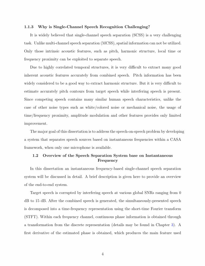
1.1.3 Why is Single-Channel Speech Recognition Challenging?
It is widely believed that single-channel speech separation (SCSS) is a very challenging
task. Unlike multi-channel speech separation (MCSS), spatial information can not be utilized.
Only those intrinsic acoustic features, such as pitch, harmonic structure, local time or
frequency proximity can be exploited to separate speech.
Due to highly correlated temporal structures, it is very difficult to extract many good
inherent acoustic features accurately from combined speech. Pitch information has been
widely considered to be a good way to extract harmonic structure. But it is very difficult to
estimate accurately pitch contours from target speech while interfering speech is present.
Since competing speech contains many similar human speech characteristics, unlike the
case of other noise types such as white/colored noise or mechanical noise, the usage of
time/frequency proximity, amplitude modulation and other features provides only limited
improvement.
The major goal of this dissertation is to address the speech-on-speech problem by developing
a system that separates speech sources based on instantaneous frequencies within a CASA
framework, when only one microphone is available.
1.2 Overview of the Speech Separation System base on InstantaneousFrequency
In this dissertation an instantaneous frequency-based single-channel speech separation
system will be discussed in detail. A brief description is given here to provide an overview
of the end-to-end system.
Target speech is corrupted by interfering speech at various global SNRs ranging from 0
dB to 15 dB. After the combined speech is generated, the simultaneously-presented speech
is decomposed into a time-frequency representation using the short-time Fourier transform
(STFT). Within each frequency channel, continuous phase information is obtained through
a transformation from the discrete representation (details may be found in Chapter 3). A
first derivative of the estimated phase is obtained, which produces the main feature used
4
in the dissertation, instantaneous frequency. Once instantaneous frequency is obtained,
pair-wise cross-channel correlation and mean square difference are both calculated as a way
to identify those frequency channels that are believed to be dominated by the same source.
A voiced/unvoiced segment detection is applied to identify the rough boundaries between
voiced and unvoiced segments. While instantaneous frequency-based features are applied in
voiced segments, amplitude-based features are used in unvoiced segments to group frequency
components from the same source. Speaker identification is applied to each processed time
frame to group the separated clusters according to speaker, so that after processing is
complete ideally only frequency channels dominated by the target speaker are extracted,
while other frequency channels believed to be from the interfering speaker are suppressed.
Finally, the reconstructed speech is sent to a speech recognizer for the final recognition task.
1.3 Dissertation Outline
This section gives a brief review of the organization of this dissertation.
In Chapter 2, some relevant previous research results in single-channel speech separation
area are briefly discussed. Because we exploit the fact that speech components from the same
source tends to vary together in terms of amplitude modulation, instantaneous amplitude
and modulation spectrogram-based methods are discussed first. Another natural way to
think about the source separation problem is that of trying to detect pitch contours from
each individual source. Multi-pitch tracking algorithms are introduced subsequently.
Chapter 3 first discusses a few ways to calculate instantaneous frequency, which is the
most important feature used in this dissertation to group speech components from the same
source. We discuss the calculation of instantaneous frequency in the context of some real
examples based on multiple sine tones, frequency-modulated complex tones, and real speech.
After calculating instantaneous frequency, the development of methods to identify correlated
frequency channels is the next step. In Chapter 4, cross-correlation-based and mean-square-error-based
methods are discussed with the goal of correlating frequency channels from the same source.
5

At the end of this chapter, one dimensional projection and graph-cut methods are proposed
as methods to extract the correlation information.
In chapter 5, two regrouping methods, pitch-based regrouping and regrouping based on
speaker identification, are introduced. Some general principles about mask generation are
discussed here as well. Finally, experimental results are presented and discussed.
While instantaneous frequency is a useful feature for voiced segments, unvoiced segments
from the same source become a little less reliable to group same source frequency components
together. In Chapter 6, both voiced/unvoiced segment detection and threshold-based time-frequency
cell suppression are discussed in detail.
Finally, Chapter 7 summarizes our work and its major conclusions. Potential future work
is also discussed.
6
CHAPTER 2REVIEW OF ALGORITHMS FOR SINGLE-CHANNEL SPEECH SEPARATION
This chapter will review several speech separation algorithms which can be used for
single-channel speech separation in the CASA framework. A general discussion of CASA and
the motivation of using CASA will be given first. Following the CASA discussion, speech
separation based on instantaneous amplitude and multi-pitch tracking will be discussed in
detail in terms of their ability to separate speech.
2.1 CASA Introduction
Computational Auditory Scene Analysis (CASA) has broad application to source separation.
Generally speaking, CASA is a wide collection of various computational implementations of
auditory scene analysis (ASA). Before a more advanced discussion of CASA is provided,
it is necessary to briefly introduce ASA and its major application. Many scientists believe
that audition shares many similarities with vision [24, 33]. The human auditory system
transforms speech into a neural representation which is then presumed to be processed in a
fashion that is similar to image processing. The entire ASA procedure can be separated
into two stages: segregation and regrouping. In the first stage, speech is decomposed
into a higher-dimensional space (such as a spectro-temporal two-dimensional representation)
where similar units (e.g., time-frequency cells in the previous 2D representation example)
are collected together into different regions. In the second stage, these regions are grouped
together into different streams based on the values of various acoustic cues or other information.
Finally, the target speech or interfering speech or both can be reconstructed for different
purposes. These functions will be discussed below in detail.
In general, CASA uses computational methods to generate a machine perception system
which may have similar functionality to that of humans. We consider primarily either one or
two microphones (the two ears of human audition). In this scenario, Wang and Brown [50]
define CASA as “the field of computational study that aims to achieve human performance
in ASA by using one or two microphone recordings of the acoustic scene.”
7

Figure 2-1 below shows a simplified diagram of a typical CASA system, where input
speech is first going through a domain transformation function. Most of the time, this
function transforms the one-dimensional speech signal into the very popular two-dimensional
time-frequency representation, either by standard short time Fourier transformation (STFT)
or a Gammatone filter bank. Following the domain transformation, the next procedure is
speech component segregation. In this part, all time-frequency cells are segmented into
different regions. All cells sitting in the same region are believed to be from the same speech
source. Various feature extraction algorithms are proposed in this stage in order to optimize
the segmentation results. The next step in the figure is described as speech component
regrouping. This stage is processed in an utterance-based format to extract all the segments
believed to be from the same speech source while suppressing all others. The most popular
such method is speaker identification. Finally, all extracted time-frequency cells are used to
reconstruct the resynthesized speech.
2.1.1 Motivation for Exploiting CASA
Speech is challenging because of its high dynamic range in both the time and frequency
domains. When competing speech is presented, the combined speech presents an even more
complicated structures that must be recognized or separated. CASA provides a good angle
to look at this problem by projecting one dimensional speech into higher dimensions. In
the following sections, discussion will be limited to the two dimensional time-frequency
representation. Due to energy sparsity, it is frequently the case that corrupted signals in the
time domain may be separable after transformation into a time-frequency representation.
To further clarify the concept of “energy sparsity”, by looking at any spectrogram of a given
speech, it is easy to discover that not every time-frequency cell plays an equally important
role in representing the information carried by the speech. A large percent of cells carrying
very low energy are much less important compared to a few percent of high-energy cells.
The transformation makes the target speech look less ”ambiguous” than it was before. As a
8
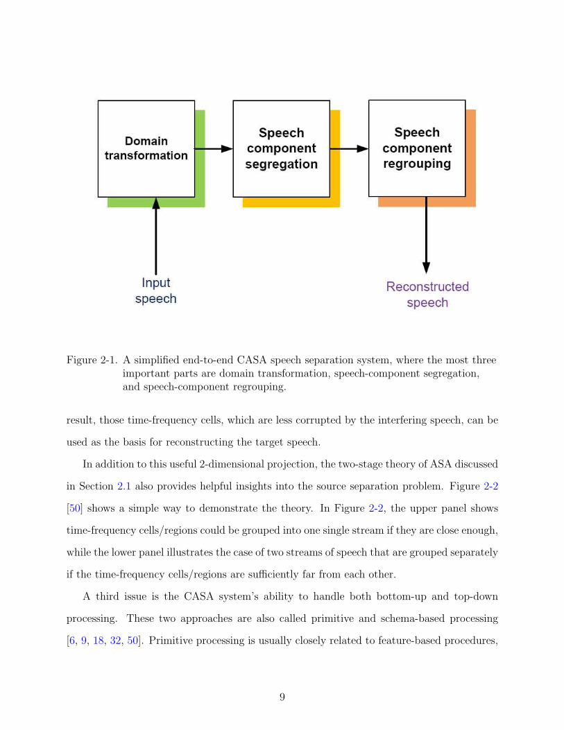
Figure 2-1. A simplified end-to-end CASA speech separation system, where the most threeimportant parts are domain transformation, speech-component segregation,and speech-component regrouping.
result, those time-frequency cells, which are less corrupted by the interfering speech, can be
used as the basis for reconstructing the target speech.
In addition to this useful 2-dimensional projection, the two-stage theory of ASA discussed
in Section 2.1 also provides helpful insights into the source separation problem. Figure 2-2
[50] shows a simple way to demonstrate the theory. In Figure 2-2, the upper panel shows
time-frequency cells/regions could be grouped into one single stream if they are close enough,
while the lower panel illustrates the case of two streams of speech that are grouped separately
if the time-frequency cells/regions are sufficiently far from each other.
A third issue is the CASA system’s ability to handle both bottom-up and top-down
processing. These two approaches are also called primitive and schema-based processing
[6, 9, 18, 32, 50]. Primitive processing is usually closely related to feature-based procedures,
9

Figure 2-2. In CASA, speech can be first projected into time-frequency cells in a 2-Drepresentation. Based on how close each time-frequency region is relative to theothers, the regions can be grouped and reconstructed into streams fromdifferent sources. How to classify each region and use various cues to groupthem into streams provides great flexibility to reconstruct target speech frominterfering sources.
such as time and frequency proximity, onset/offset detection, smoothness of pitch or formant
trajectory, periodicity, etc. Human beings have the ability of accumulating knowledge
gradually after they are first born. The learning procedure generates many patterns, or
prior knowledge. Those stored patterns help to interpret corrupt patterns in many different
scenarios. In source separation, when certain parts of speech in the 2-D representation
become discontinuous due to the presence of competing speech, human beings tend to use a
priori knowledge to fill the gaps in the representation and recover the speech to its maximum
intelligibility.
2.1.2 Examples of CASA Systems and Applications
CASA systems have been widely used in many different applications. Below is a limited
collection of several examples [50].
• Robust automatic speech and speaker recognition
• Hearing prostheses
• Automatic music transcription
• Audio information retrieval
10

• Auditory scene reconstruction
In this dissertation, the discussion of CASA systems will be limited to the application of
monaural speech separation.
Projecting time-domain speech into the time-frequency domain is generally considered
to be the first step towards solving the problem. The short-time Fourier Transform (STFT)
and Gammatone filterbank are both considered to be proper vehicles to implement the
transform. In STFT, the center frequencies of each frequency channel are separated by the
same difference in frequency. For each fixed time frame, the frequency response is the Fourier
transform of that given time frame. While each frequency channel is fixed, the output of each
channel can be considered as a filter output of a specific bandpass filter. In the application
of Gammatone filtering, the spacing of the center frequency of each channel varies with
frequency. This provides better frequency resolution for low frequencies at the expense of
worse spectral resolution for high frequencies.
After the transformation is done, an attempt is made to determine which time-frequency
cells are believed to have similar characteristics. This step is usually done by applying
different intrinsic acoustic cues. The next step is that of regrouping different time-frequency
regions into different streams to reconstruct either target speech, interfering speech or both.
In this stage, the most popular method used is speaker identification based on the training
data, from which each speaker’s acoustic characteristics are learned by the system. In the
reconstruction procedure, the a posteriori probability of each speaker in the training pool is
calculated for each time frame to get the best match. Based on speaker identification results,
further extraction or suppression is performed to generate different speech streams.
2.1.3 CASA Mask Generation and Evaluation
A key part of both the segmentation and regrouping stages of CASA systems is mask
generation. The term mask generation generally refers to the judgement of each individual
time-frequency cell or region whether they are reliable or not. “Reliable” here generally
means the time-frequency cell belongs to the target speaker. A “binary masks” is made about
11

whether each time-frequency cell is reliable or unreliable, while the cells of “continuous”
masks are assigned a probability of reliability. The final construction of either target or
competing speech is performed based on these values.
There are various ways of evaluating the CASA systems. In this section, several popular
assessments are briefly listed.
Word Error Rate (WER): In this method, the reconstructed speech is fed into a speech
recognizer for automatic speech recognition. WER can be used as an objective assessment
to value different separation algorithms, where the best approaches yield the lowest WER
value.
Spectrogram Distance: Another way to assess separation algorithm is spectrogram
distance. In the method, the spectrogram of reconstructed speech is compared with the
original clean speech. The smaller the distance between these spectrograms, the better the
separation algorithm is.
Mean Opinion Score (MOS): The Mean Opinion Score (MOS) is a very popular
subjective evaluation scheme using human subjects. In this method, professional personnel
are asked to score to each reconstructed speech utterance on a scale of 1 to 5, from the worst
to the best.
We will use WER exclusively as the standard of evaluation of the success of the various
separation algorithms considered.
2.2 Amplitude-Modulation Spectral Analysis
In many analyses [1, 4, 7, 8, 39, 41] it is useful to separate speech and music signals into
two parts, a low-frequency modulating signal and a higher-frequency modulated carrier [39,
41]. Equations 2.1 and 2.2 describle a single-component modulation and a multi-component
modulated signal, respectively.
x(t) = m(t)c(t) (2.1)
12
x(t) =N∑
n=1
sn(t) =N∑
n=1
mn(t)cn(t) (2.2)
where x(t) is the single-component or multi-component signal, m(t) or mn(t) are the low-frequency
modulating signals and c(t) or cn(t) are the high-frequency carriers.
Many researchers believe that the modulator of a speech signal is more important than its
own carrier signal in terms of speech perception. When a real modulator signal is replaced
by a constant envelope, speech becomes unintelligible. On the contrary, if the carrier is
replaced by white noise but the modulator signal is untouched, the speech remains very
intelligible. This observation has led many researchers to apply amplitude modulation to
monaural source separation with the hope of making amplitude modulation an important
intrinsic acoustic feature.
A popular implementation of this idea is the decomposition of the original signal into
many narrowband frequency subbands. Within each subband, the signal is further decomposed
into a modulator and a carrier. Then various feature-extraction methods based on this
implementation are used to further group components from the same source together.
2.2.1 Amplitude Modulation based Algorithms
The use of long-term temporal features to improve speech recognition accuracy has been
shown to be successful by a number of research groups (e.g. [25]). For example, Atlas and his
colleagues (among others) have proposed the use of modulation spectral analysis as a tool to
separate mixed speech in higher-dimensional spaces [40] [2]. The time-domain signal is first
transformed into a time-frequency representation by applying Short-time Fourier Transfomr
(STFT). Then, the instantaneous amplitude is calculated for each narrow-band frequency
bin. Conventional coherent demodulation is accomplished through the use of the Hilbert
transform approach. An improved “coherent demodulation” [28], which removes the carrier
frequency (i.e. the center frequency of each bandpass filter) to a high degree, has been shown
to provide better performance in term of extracting the envelope. A second FFT for the
new estimated envelope is calculated within each frequency bin. If the envelope is indeed
13

modulated at a certain frequency, the FFT operation will produce a spike at that frequency,
which is also called the modulation frequency. This process is depicted in Figure 2-3 [40]
Figure 2-3. The speech signal is first decomposed into a time-frequency representation bySTFT. Then within each frequency channel, a second FFT is calculated totransfer to time-frequency representation to a frequency-frequencyrepresentation, where one frequency axis represents physical frequency and theother frequency axis represents modulation frequency.
Modulation-spectral theory assumes that natural speech is modulated at a rate from 2 to
20 Hz. While mixed speech may have a great deal of overlap in the time domain, modulation
frequency analysis provides an additional dimension that can provide a greater degree of
separation among sources. In other words, the original time-frequency representation obtained
from analyses such as STFT can be augmented to a third dimension representing modulation
frequency. Components of signals from a common source are more likely to exhibit the
14
same modulation frequency. By selecting non-overlapped elements according to modulation
frequency and regrouping them together, the target speech can in principle be reconstructed
and used either for speech enhancement or speech recognition.
Nevertheless, this approach has its own issues. Since modulation frequency usually is
low (again on the order of 5 to 20 Hz), a long time window is needed to estimate frequency
components reliably. (For example, a 5-Hz signal typically requires an analysis frame of
more than 200 ms in duration to capture the frequency components of this slowly-varying
signal.) This is a problem because it is well known that instantaneous frequency changes are
important for the final recognition result, and that long temporal windows will cause these
frequency changes to be averaged out. This problem is similar to the tradeoff between time
and frequency resolution in conventional STFT. In addition, the “coherent demodulation”
method described by [28] requires an estimate of the concentrated frequency energy for each
predefined frequency block. An incorrect estimation will lead to the wrong carrier frequency
and will adversely affect the quality of the envelope that is estimated.
2.2.2 Differences between Amplitude and Frequency Modulation Schemes
Although amplitude and frequency modulation schemes are different, it is worthwhile to
compare their mathematical details and make a few comparisons. Equation 2.3 describes a
signal that could have both amplitude and frequency modulation.
y(t) = m1(t) cos(θ(t)) = m1(t) cos(ω0t +
∫ t
0
m2(τ)dτ + θ0) (2.3)
In Equation 2.3, m1(t) represents the amplitude modulation, where m2(t) represents the
frequency modulation. When m2(t) is equal to zero, the signal is completely modulated
by amplitude modulation. While m1(t) is equal to zero, the signal is only modulated by
frequency modulation.
In practice, coherent amplitude modulation is not very easy to obtain. Errors incurred in
the process of amplitude estimation will contribute severe negative effects to the next step
regardless of whether the modulation spectrogram or adjacent correlation patterns are used.
15

While it is not possible to get a perfect estimate of instantaneous frequency, the results in the
following chapters will show that instantaneous frequency can be used directly without very
strict accuracy requirements to obtain better WER that can be obtained from instantaneous
amplitude estimation.
2.3 Multi-Pitch Tracking based Speech Separation
It is very natural to imagine that speech separation can be accomplished by detecting
the pitch of the mixed speech. Generally speaking, pitch estimation can be done using either
temporal, spectral or spectro-temporal methods [3, 10, 20]. Unfortunately, it is very difficult
to obtain perfect pitch estimation due to mutual interference from the harmonic structure of
each speaker, and a reliable algorithm that can detect each of several simultaneously-presented
pitches is critical in this approach. Figure 2-4 [50] shows that determining F0 by looking at
global or local maxima from spectra from pure or complex tones may not be very promising
without further complicated modification. If we could identify the pitch contours of each of
several simultaneous speakers, comb filtering or other techniques could be used to select the
frequency components of the target speaker and suppress other components from competing
speakers.
Because of its straightforward physical meaning and overall appeal, a great deal of effort
has been put into algorithms that accomplish multi-pitch detection (e.g. [51], [21], [15],
[30] and [5]). Weintraub’s system [30] was among the first algorithm in this field that
was applied to speech recognition. Weintraub computed the autocorrelation function of
cochlear outputs, and used dynamic programming (DP) to estimate the dominant pitch
from these results. After removing the components from the dominant speaker, this process
was repeated to retrieve the pitch values from the weaker speaker. This method is simple and
easy to implement, but it does not generally lead to a satisfactory reduction in word error
rate. In addition, a Markov model is used to estimate whether zero, one, or two speakers
are speaking simultaneously, and this classifier must be trained from data from the same
16

Figure 2-4. In this figure, panel (a) shows a pure tone with period T. The correspondingspectra peak is also shown on the right. Panels (b), (c), (d) and (e) share thesame period T of the signal in panel (a) with different waveforms. However, bylooking at the spectral response on the right, it is truly difficult to determinethe fundamental frequency simply by locating the position of the global spectrapeak.
speakers, which may not always be available. Other researchers [15] [14] have proposed
similar recursive cancelation algorithms in which the dominant pitch value is first estimated,
and then removed so that a second pitch value can be calculated. All of these algorithms
are critically dependent on the performance of the first estimation stage, and errors in the
first pass usually lead to errors in all subsequent passes.
Hu and Wang (e.g. [21]) have used a different approach to estimate pitch from simultaneously-presented
speech, and their algorithm has the additional advantage of performing voiced/unvoiced
decisions at the same time. A block diagram of this procedure is shown in Figure 2-5.
They begin by calculating correlograms of the outputs of a model of peripheral auditory
17
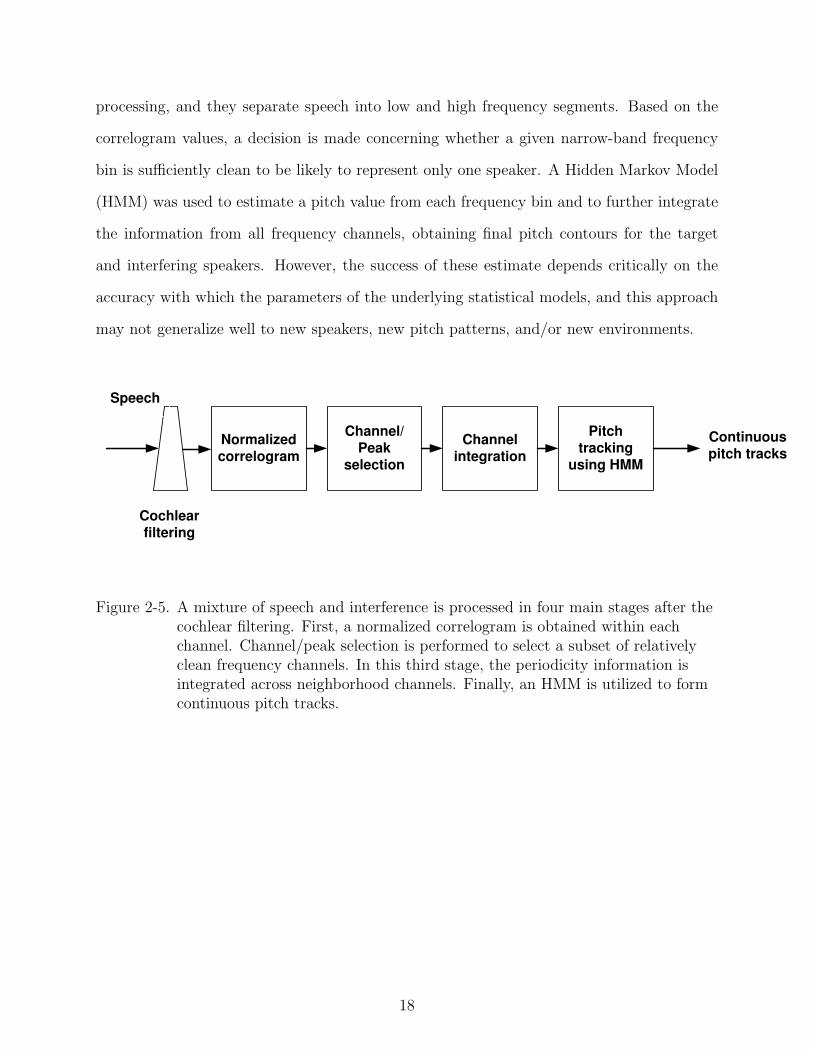
processing, and they separate speech into low and high frequency segments. Based on the
correlogram values, a decision is made concerning whether a given narrow-band frequency
bin is sufficiently clean to be likely to represent only one speaker. A Hidden Markov Model
(HMM) was used to estimate a pitch value from each frequency bin and to further integrate
the information from all frequency channels, obtaining final pitch contours for the target
and interfering speakers. However, the success of these estimate depends critically on the
accuracy with which the parameters of the underlying statistical models, and this approach
may not generalize well to new speakers, new pitch patterns, and/or new environments.
Normalized
correlogram
Channel/
Peak
selection
Channel
integration
Pitch
tracking
using HMM
Continuous
pitch tracks
Speech
Cochlear
filtering
Figure 2-5. A mixture of speech and interference is processed in four main stages after thecochlear filtering. First, a normalized correlogram is obtained within eachchannel. Channel/peak selection is performed to select a subset of relativelyclean frequency channels. In this third stage, the periodicity information isintegrated across neighborhood channels. Finally, an HMM is utilized to formcontinuous pitch tracks.
18

CHAPTER 3ESTIMATION OF INSTANTANEOUS FREQUENCY AND ITS APPLICATION TO
SOURCE SEPARATION
This chapter introduces a new temporal feature based on instantaneous frequency that
is intended to address some of the drawbacks to the approaches that were discussed in the
previous chapter. In the early days of research, the ways in which the human auditory system
interprets basic stimuli have been carefully studied by many researchers [47–49, 52–54]. As
in the case of many other signal processing concepts, instantaneous frequency was originally
considered in the context of frequency modulation (FM) theory that has been used in many
types of communications systems. One of the most important concepts is the observation
that the spectral characteristics of many real signals are not constant over time [7, 8]. Signal
containing these characteristics are considered to be non-stationary. A simple example is the
chirp signal, where the instantaneous frequency is a linear function of time as in Figure 3-1.
For speech signals, instantaneous frequency is also an important characteristic. It is a
time-varying parameter which defines the location of the signal’s spectral peak as it varies
with time. Theoretically speaking, it can be interpreted as the frequency of the best fit
to the signal under analysis [7, 8]. This analysis assumes that the signal contains only a
single frequency in the analysis band. Multi-component signals must first be decomposed
into many narrow-band ranges for further processing.
Many research results [9] have shown that the frequency components of human speech
tend to be modulated in the frequency range of 2 Hz to 20 Hz. The carrier frequencies of
voiced speech segments are usually harmonically related, and modulated by a modulation
frequency in the range discussed above. This implies that the frequency deviation, which
refers to the amplitude of the instantaneous frequency, is proportional to the harmonic
number.
3.1 Modulation Frequency and Its application to Speech Separation
There are many different types of inherent information contained in speech, such as
pitch, onset/offset, time/frequency continuity, etc, as noted in Chapter 2. Among all the
19

Time
Fre
quen
cyChirp signal
0 0.1 0.2 0.3 0.4 0.5 0.6 0.7 0.8 0.90
1000
2000
3000
4000
5000
6000
7000
8000
Figure 3-1. Spectrogram of a chirp signal whose frequency increases linearly with time.
various features, long-term temporal features are worthy of great attention. Among these
long-term temporal features, in addition to instantaneous frequency, the similar concept
of modulation frequency has also been the subject of much attention and have been used
to detect pitch, separate speech, and modify speech. While instantaneous frequency and
modulation frequency are related, they are not exactly the same. Modulation frequency
is independent of both frequency modulation or amplitude modulation, and simply refers
to the reciprocal of an entire period of a slow time-varying modulating signal. Figure
3-2 demonstrates the concepts of modulation frequency and instantaneous frequency. As
discussed above, the instantaneous frequency is the entire waveform shown in Figure 3-2,
while the reciprocal of the period of a given instantaneous frequency is the modulation
frequency.
20

0 0.2 0.4 0.6 0.8 11980
1985
1990
1995
2000
2005
2010
2015
2020
Time
Phy
sica
l fre
quen
cyInstantaneous frequency
modulationperiod
frequencydeviation
Figure 3-2. A simple example compares the concepts of modulation frequency, deviationfrequency, and instantaneous frequency. In the figure, the modulationfrequency is 5 Hz, the deviation frequency is 20 Hz. The modulation period is200 ms, the reciprocal of the modulation frequency of 5 Hz.
Many studies have focused on modulation frequency in the fields of psychoacoustics
and speech production, and it is now beginning to be exploited for speech processing and
recognition. For example, the impact of modulation frequency on speech recognition was
discussed in [46]. Filter design based on modulation frequency has also been proposed for
preprocessing to mitigate the effects of reverberation [26]. Modulation frequency can also be
combined with nonnegative matrix factorization to estimate pitch explicitly [42].
The potential exploitation of modulation frequency can contribute greatly to improved
source separation. Traditional signal processing techniques such as short-time Fourier transform
(STFT) separate signals according to time and frequency. If modulation frequency can be
21
consistently extracted, it provides a potential third orthogonal dimension along which signal
components can be separated and clustered. The target speech signal can potentially be
reconstructed by selecting those localized time-frequency regions that exhibit a particular
common modulation frequency [40]. Nevertheless, accurate estimation of modulation frequency
can be quite difficult for natural signals as discussed in Chapter 2.
In this chapter instantaneous frequency will be the main focus of discussion.
3.2 Instantaneous Frequency and Its Calculation
A narrowband signal can be represented by a higher-frequency carrier modulated in
amplitude and phase at lower frequencies. While there are many different ways to calculate
the instantaneous frequency, the primary way is to take the first derivative of the phase
information. In this section, several different methods of calculating instantaneous frequency
will be discussed.
3.2.1 Instantaneous Frequency Calculation
Consider, for example, the continuous-time representation of a sinusoid with time-varying
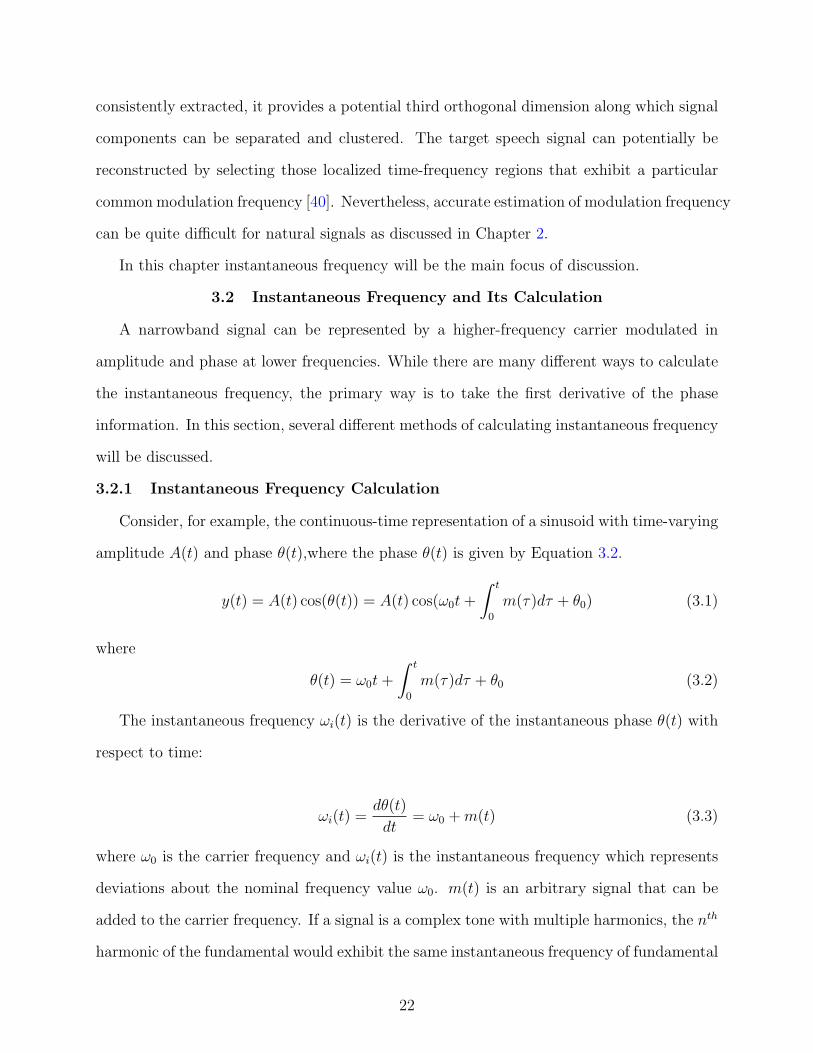
amplitude A(t) and phase θ(t),where the phase θ(t) is given by Equation 3.2.
y(t) = A(t) cos(θ(t)) = A(t) cos(ω0t +
∫ t
0
m(τ)dτ + θ0) (3.1)
where
θ(t) = ω0t +
∫ t
0
m(τ)dτ + θ0 (3.2)
The instantaneous frequency ωi(t) is the derivative of the instantaneous phase θ(t) with
respect to time:
ωi(t) =dθ(t)
dt= ω0 + m(t) (3.3)
where ω0 is the carrier frequency and ωi(t) is the instantaneous frequency which represents
deviations about the nominal frequency value ω0. m(t) is an arbitrary signal that can be
added to the carrier frequency. If a signal is a complex tone with multiple harmonics, the nth
harmonic of the fundamental would exhibit the same instantaneous frequency of fundamental
22

frequency multiplied by n:
ωn(t) = nω0 + nm(t) (3.4)
Because instantaneous frequency is a concept that is meaningful only for narrowband
signals as discussed above, an incoming speech signal must be passed through a bank
of bandpass filters to provide parallel narrowband components from which instantaneous
frequency may be estimated. In addition, this processing normally must take place in discrete
time. The short-time Fourier transform (STFT) provides a convenient way to obtain this
bandpass filtering implicitly [16, 19, 34, 37]. The combined speech x[n] is decomposed into
the two-dimensional time-frequency representation X[n, k] where n is the time frame index
and k is the index of frequency bins. Each frequency bin can be considered to be the output
obtained by passing the original input through a narrow bandpass filter. The instantaneous
amplitude and phase of the filter outputs for each frequency bin will be slowly time varying.
The phase information θ[n, k] is obtained easily from the inverse tangent of the quotient of
the imaginary and real parts of the filter output X[n, k]:
θ[n, k] = arctan(=(X[n, k])
<(X[n, k])) (3.5)
The instantaneous frequency ω[n, k] is estimated by taking the first difference of the instantaneous
phase, with care taken to deal appropriately with the effects of phase wrapping.
ω[n, k] = θ[n, k]− θ[n− 1, k] (3.6)
In [19, 37], an alternative calculation was proposed as follows. Suppose X(ωn, t) is the
time frequency representation of a given signal x(n) obtained by applying Short-Time Fourier
Transform (STFT). X(ωn, t) can then be represented in Equation 3.7, where a and b are the
corresponding real and imaginary parts of the complex spectrum.
X(ωn, t) = a(ωn, t)− jb(ωn, t) (3.7)
23

where
a(ωn, t) =
∫ t
−∞x(τ)h(t− τ) cos(ωnτ)dτ (3.8)
and
b(ωn, t) =
∫ t
−∞x(τ)h(t− τ) sin(ωnτ)dτ (3.9)
From these equations the instantaneous frequency can be calculated as follows:
d(θ(ωn, t))
dt=
(da/dt)b− (db/dt)a
a2 + b2(3.10)
In the actual calculation of instantaneous frequency, all the work must be done in the
discrete domain. Equation 3.8 and 3.9 can be represented in their discrete form as in
Equation 3.11 and 3.12
a[ωn,m] = Σml=0x[l] cos[ωnl]h[m− l] (3.11)
b[ωn,m] = Σml=0x[l] sin[ωnl]h[m− l] (3.12)
Again, m is the frame index along the time axis. Simply by taking the first-order difference
of Equation 3.11 and 3.12, ∆a and ∆b can be calculated:
∆a = a[ωn, (m + 1)]− a[ωn,m] (3.13)
∆b = b[ωn, (m + 1)]− b[ωn,m] (3.14)
Finally, the discrete form of instantaneous frequency can be calculated in Equation 3.15:
∆ϕ
T[ωn,mT ] =
1
T
b∆a− a∆b
a2 + b2(3.15)
where T is the sampling period to collect the signal. Before other alternative ways to calculate
instantaneous frequency introduced in the following section, Figure 3-3 is a block diagram
24

that describes how to obtain instantaneous frequency in the original way as discussed above.
Figure 3-3. A block diagram that describes how instantaneous frequency is calculated bythe method discussed in Equation 3.6.
Although the schemes shown in Figures 3-3 and 3-4 are perfect for continuous signals,
some practical issues arise when discrete signals are involved. Equation 3.16 shows a discrete
Short-Time Fourier Transform:
X[n, k] =∞∑
m=−∞x[m]w[n−m]e
−j2πmkN (3.16)
where n is the frame index and k is the frequency index. Therefore, the phase information
and thus the corresponding instantaneous frequency calculated from Equation 3.6 and 3.15
are all functions of n and k. Every instantaneous phase calculated here is the difference
between an average version of all samples included in the current frame and its neighbor.
More specifically, the instantaneous phase calculated in the discrete case is dependent on
25

Figure 3-4. A block diagram that describes how instantaneous frequency is calculated byusing the method discussed in Equation 3.15.
26

three factors. The first is the length of the analysis window. The second is the shape of the
analysis window. And the third is the overlap between adjacent windows. The last factor
gives us a hint that the calculated instantaneous phase may result in an unnecessary phase
discontinuity. In other words, the adjacent phase difference can jump out of the range of π.
In this case, phase unwrapping is often done by adding multiples of ±2π to limit the change
of phase over successive frames. Figure 3.2.1 demonstrates how phase unwrapping works.
[FIX FIG REF]
However, phase unwrapping only partially solves the problem. The following example
shows that the calculations based on both Equations 3.6 and 3.15 give the wrong phase of
the estimated instantaneous frequency.
x(t) = Acos(θ(t)) (3.17)
θ(t) = 2πfct +20
fm
sin(2πfmt) (3.18)
ω(t) = 2πfc + 2π20 cos(2πfmt) (3.19)
Equation 3.18 and 3.17 illustrate an expression of a testing signal, in which the instantaneous
frequency is given in Equation 3.19. However, Figure 3-6 shows that the instantaneous
frequency from all three channels in the harmonic structure contains instantaneous frequency
in the form of a sine wave rather than a cosine, even though the frequency deviation and
modulation frequency value are correct in this example.
In the following section, two “continuous” forms of instantaneous frequency calculation
will be presented in order to solve this problem, where “continuous” refers to avoiding using
the phase difference between adjacent windows in the discrete case.
27
100
−2
−1.5
−1
−0.5
0
0.5
1
1.5
2
ω
Rad
ian
phas
e
Phase before unwrap
Original jump3.5873 radians
A Before phase unwrapping, a wide phase jump exists
100
−5
−4.5
−4
−3.5
−3
−2.5
−2
−1.5
ω
Rad
ian
phas
e
Phase after unwrap
Corrected jump2.6959 radians
B After phase unwrapping, the wide phase jump is removed
Figure 3-5. The upper panel is the estimated phase before phase unwrapping and the lowerpanel is the corresponding estimate after phase unwrapping.
3.2.2 Two Alternative ways to Calculate Instantaneous Frequency
As discussed in the previous section, assume X(ω, t) is the time frequency representation
of a given signal x(n) in the time domain. An alternate representation of X(ω, t) is in the
form of Equation 3.20 below:
28

0 0.2 0.4 0.6 0.8 11980
2000
2020Instantaneous frequency for three harmonic related channels
0 0.2 0.4 0.6 0.8 13950
4000
4050
Fre
quen
cy
0 0.2 0.4 0.6 0.8 15900
6000
6100
Time
Figure 3-6. The instantaneous frequency estimate of a multi-sinusoid signal usingEquations 3.6 or 3.15.
X(ω, t) = A(ω, t)ejθ(ω,t) (3.20)
where A(ω, t) is the instantaneous amplitude and θ(ω, t) is the instantaneous phase information.
Since instantaneous frequency is related only to its instantaneous phase, the phase can be
calculated as in Equation 3.22 [27]:
θ(ω, t) = ∠X(ω, t) = =log[X(ω, t)] (3.21)
where ∠x and =x denote the angle and the imaginary part of the complex number x,
respectively.
29
∂θ(ω, t)
∂t=
∂=(log[X(ω, t)])
∂t
= =(∂ log[X(ω, t)]
∂t)
= =(∂X(ω, t)/∂t
X(ω, t))
= =(∂∂t
∫∞−∞ x(τ)w(τ − t)e−jωτdτ
X(ω, t))
= =(
∫∞−∞ x(τ)∂w(τ−t)
∂te−jωτdτ
X(ω, t))
= =(X1(ω, t)
X(ω, t)) (3.22)
where X(ω, t) is the Short-Time Fourier Transform (STFT) of the time domain signal x(n)
and X1(ω, t) is the STFT of the same signal x(n) but using the derivative of the original
window w(t) as the new window signal. Equation 3.23 and 3.24 show details below:
X(ω, t) =
∫ ∞
−∞x(τ)w(τ − t)e−jωτdτ (3.23)
X1(ω, t) =
∫ ∞
−∞x(τ)
∂w(τ − t)
∂te−jωτdτ (3.24)
Equation 3.22 does not calculate instantaneous frequency through each windowed frame.
Instead, it takes the derivative of the window signal itself and calculates instantaneous
frequency in a “continuous” way while remaining in discrete form. By using this method,
there is no first-order discrete difference operation needed to calculate instantaneous frequency.
All calculations are based on the same operation of the STFT with a different type of window
signal.
Given the time-frequency representation of signal x(n) in Equation 3.23, the filter bank
can be expressed in Equation 3.25:
F (ω, t) = ejωtX(ω, t) (3.25)
30
As a result, the instantaneous frequency can be represented by Equation 3.26 :
∂θ(ω, t)
∂t=
∂
∂targ[F (ω, t)] (3.26)
If F (ω, t) is also represented as:
F (ω, t) = a− jb (3.27)
Inspired by Equation 3.10,
∂θ(ω, t)
∂t=
(∂a/∂t)b− (∂b/∂t)a
a2 + b2(3.28)
To solve ∂a/∂t and ∂b/∂t in a “continuous” way, we perform the operation
∂
∂tF (ω, t) =
∂a
∂t− j
∂b
∂t
=
∫ ∞
−∞(−∂w(τ − t)
∂t+ jωw(τ − t))e−jw(τ−t)x(τ)dτ (3.29)
In Equation 3.29, it is easy to see the equation is nothing but a STFT of the same
signal x(n). Again, the only difference is the window signal w(τ − t) is replaced by a new
window −∂w(τ−t)∂t
+jωw(τ−t). By doing this transformation, all parameters in Equation 3.28
can be calculated in “continuous” form and thus achieve the best possible results. Figure
3-8 illustrates the estimate of instantaneous frequency obtained by using the instantaneous
phase represented by Equation 3.18. By contrasting it to Figure 3-6, it is easy to see that this
estimate has the correct cosine form with the correct deviation and modulation frequencies.
3.3 Instantaneous Frequency Estimation for Frequency-modulated ComplexTone
In the previous sections we discussed methods for estimating instantaneous frequency
in both continuous and discrete form. We now discuss some actual examples using a
multi-sinusoidal signal, along with the estimation of instantaneous frequency for frequency-modulated
complex tones.
31

speech
Re(k, n) Re(k, n)
Im(k, n) Im(k, n)
(Re(k, n))
(Im(k, n))
/-
+
×
×
×
×
Re(k, n) Re(k, n)
Im(k, n) Im(k, n)
(Re(k, n))
(Im(k, n))
/-
+
×
×
×
×
Differentiat
ed window
Channel 1
Channel N
IF calculation
Instantane
ous
frequency
window
STFT
STFT
(Re(k, n))
(Im(k, n))
Re(k, n),
Im(k, n)
Figure 3-7. A general diagram of how instantaneous frequency is calculated by using thedifferentiated window method discussed in Equation 3.29.
3.3.1 Frequency-modulated Complex Tones
John Chowning is a pioneer in electronic music who is perhaps best known as the father of
FM synthesis. Around 1982, Chowning demonstrated the importance of micro-modulation
in perceptual grouping of complex tones. Figure 3-9 shows the waveform we refer to as the
sum of three frequency-modulated complex tones, where each tone has its own fundamental
frequency with its own corresponding instantaneous frequency. In the figure, from left
to right, the number of complex tones increased gradually from one to three, and the
fundamental frequencies of each of the three complex tones undergo separate micro-modulations
32

0 0.2 0.4 0.6 0.8 11980
2000
2020Instantaneous frequency for three harmonic related channels
0 0.2 0.4 0.6 0.8 13950
4000
4050
Fre
quen
cy
0 0.2 0.4 0.6 0.8 15900
6000
6100
Time
Figure 3-8. The instantaneous frequency estimation from a multi-sinusoid signal usingcontinuous window derivative methods.
in frequency.
3.3.2 Extracting Instantaneous Frequency from Frequency-modulated ComplexTones
Figure 3-10 illustrates a simple example of the estimation of instantaneous frequency
from a frequency-modulated complex tone. In this example, the signal consists of two
complex tones at 0 dB, where the target tone has a fundamental frequency at 300 Hz with
5-Hz modulation frequency and 10-Hz frequency deviation, while the interfering tone has
a fundamental frequency at 400 Hz with 3-Hz modulation frequency and 15-Hz frequency
deviation. The figure shows the instantaneous frequency estimated from frequency channels
corresponding to the first and second harmonics and a third irrelevant channel, respectively.
33

Time
Fre
quen
cyChowning signal with three complex tones
0 1 2 3 4 5 6 70
1000
2000
3000
4000
5000
6000
7000
8000
Figure 3-9. Spectrogram of the sum of three frequency-modulated complex tones.
It is clear that the instantaneous frequencies from these correlated channels behave in a
similar fashion, while harmonic members’ behavior are quite different from non-harmonic
member’s. While the estimation is not perfect compared with ground truth (which would
be a perfect sinusoid), the correlation of those related channels would still be identified
using traditional cross-channel correlation methods, as discussed in the following chapters.
Without too much discussion on the cross-channel correlation methods itself, Table 3-1
shows the experimental results of comparisons among harmonic members as well as the ones
between harmonic members and non-harmonic member. In this experiment, instantaneous
frequencies are estimated from three channels at various SNRs. Two of these three channels
correspond to harmonic members, while the other is from the pool of non-harmonic channels.
The second column in the table shows the correlation value among the two harmonic members.
34
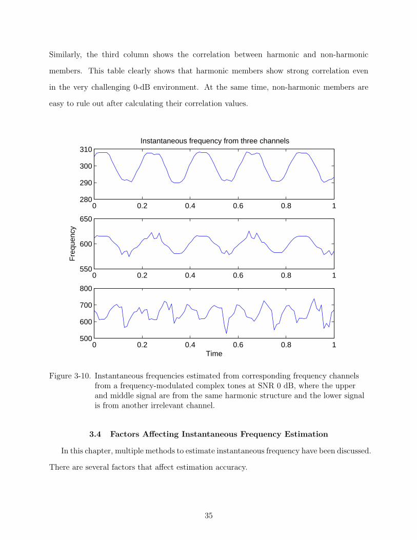
Similarly, the third column shows the correlation between harmonic and non-harmonic
members. This table clearly shows that harmonic members show strong correlation even
in the very challenging 0-dB environment. At the same time, non-harmonic members are
easy to rule out after calculating their correlation values.
0 0.2 0.4 0.6 0.8 1280
290
300
310Instantaneous frequency from three channels
0 0.2 0.4 0.6 0.8 1550
600
650
Fre
quen
cy
0 0.2 0.4 0.6 0.8 1500
600
700
800
Time
Figure 3-10. Instantaneous frequencies estimated from corresponding frequency channelsfrom a frequency-modulated complex tones at SNR 0 dB, where the upperand middle signal are from the same harmonic structure and the lower signalis from another irrelevant channel.
3.4 Factors Affecting Instantaneous Frequency Estimation
In this chapter, multiple methods to estimate instantaneous frequency have been discussed.
There are several factors that affect estimation accuracy.
35

SNR correlation between harmonics correlation with non-harmonicClean 0.9999 0.101120 dB 0.9996 0.099415 dB 0.9991 0.098110 dB 0.9976 0.09545 dB 0.9928 0.09040 dB 0.9776 0.0823
Table 3-1. Correlation comparison among harmonic members and between harmonic andnon-harmonic members.
The STFT is a popular method to project the one-dimensional time signal into a two-dimensional
time-frequency representation. In this representation, the center of each frequency channel
is linearly spaced across the whole frequency range with bandwidth overlapping depending
on how many frequency channels are used in the application. Several issues may cause
inaccuracy of estimating the final instantaneous frequency. As discussed above, as the order
of harmonics increases, the corresponding frequency deviation also increases proportionally.
This is not an issue when harmonics are in the low frequency range. Unfortunately, this
becomes a serious problem when frequency becomes greater. Since the bandwidth of each
frequency channel is only determined by the number of samples contained in each frame
used to do the Fourier transform, bandwidth is not a function of the order of harmonics.
Therefore, when the frequency deviation becomes larger than the bandwidth of the frequency
channel in the high-frequency range, the estimation of instantaneous frequency is no longer as
accurate as in the low frequency range. Fortunately, the experiments shown in the following
chapters will demonstrate that it is possible to obtain reasonable results by dealing only with
frequency components up to 4000 Hz.
The second issue of estimation comes from corruption by frequency components from
other sources. When more than one source is involved in the same mixed signal, instantaneous
frequency estimation cannot be perfect due to either noisy components sitting in the same
frequency channel or due to smearing from adjacent frequency channels. Nevertheless, Table
3-1 indicates that imperfect estimation of instantaneous frequency can still yield reasonably
good classification results.
36

In general, our proposed method is valid when the target signal does not fall below
0 dB compared to interfering speech, when the fundamental frequencies of the target and
interfering speakers are not too close to one another, limiting processing to frequencies below
4000 Hz. Fortunately, in practice, all these conditions are not too difficult to meet.
37
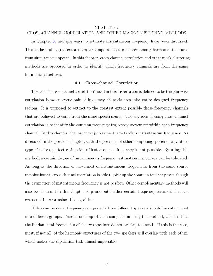
CHAPTER 4CROSS-CHANNEL CORRELATION AND OTHER MASK-CLUSTERING METHODS
In Chapter 3, multiple ways to estimate instantaneous frequency have been discussed.
This is the first step to extract similar temporal features shared among harmonic structures
from simultaneous speech. In this chapter, cross-channel correlation and other mask-clustering
methods are proposed in order to identify which frequency channels are from the same
harmonic structures.
4.1 Cross-channel Correlation
The term “cross-channel correlation” used in this dissertation is defined to be the pair-wise
correlation between every pair of frequency channels cross the entire designed frequency
regions. It is proposed to extract to the greatest extent possible those frequency channels
that are believed to come from the same speech source. The key idea of using cross-channel
correlation is to identify the common frequency trajectory movement within each frequency
channel. In this chapter, the major trajectory we try to track is instantaneous frequency. As
discussed in the previous chapter, with the presence of other competing speech or any other
type of noises, perfect estimation of instantaneous frequency is not possible. By using this
method, a certain degree of instantaneous frequency estimation inaccuracy can be tolerated.
As long as the direction of movement of instantaneous frequencies from the same source
remains intact, cross-channel correlation is able to pick up the common tendency even though
the estimation of instantaneous frequency is not perfect. Other complementary methods will
also be discussed in this chapter to prune out further certain frequency channels that are
extracted in error using this algorithm.
If this can be done, frequency components from different speakers should be categorized
into different groups. There is one important assumption in using this method, which is that
the fundamental frequencies of the two speakers do not overlap too much. If this is the case,
most, if not all, of the harmonic structures of the two speakers will overlap with each other,
which makes the separation task almost impossible.
38
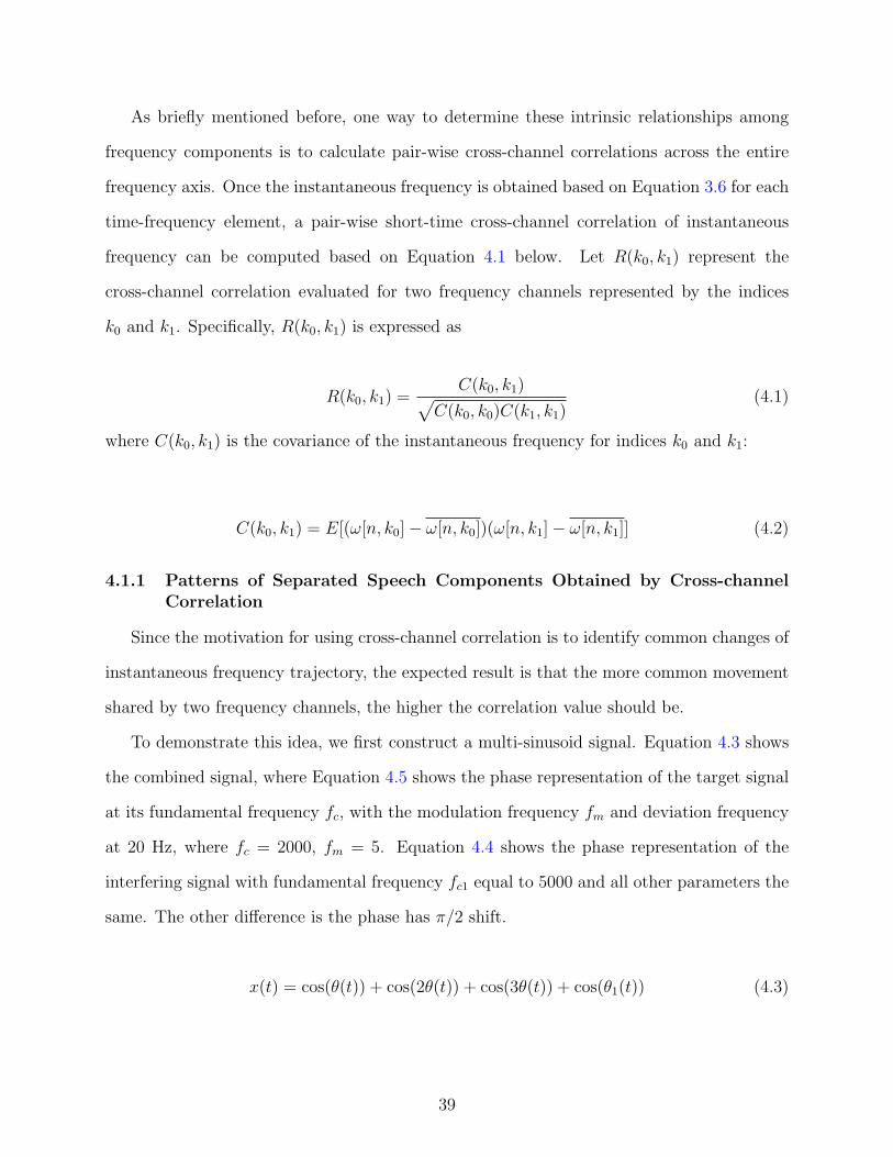
As briefly mentioned before, one way to determine these intrinsic relationships among
frequency components is to calculate pair-wise cross-channel correlations across the entire
frequency axis. Once the instantaneous frequency is obtained based on Equation 3.6 for each
time-frequency element, a pair-wise short-time cross-channel correlation of instantaneous
frequency can be computed based on Equation 4.1 below. Let R(k0, k1) represent the
cross-channel correlation evaluated for two frequency channels represented by the indices
k0 and k1. Specifically, R(k0, k1) is expressed as
R(k0, k1) =C(k0, k1)√
C(k0, k0)C(k1, k1)(4.1)
where C(k0, k1) is the covariance of the instantaneous frequency for indices k0 and k1:
C(k0, k1) = E[(ω[n, k0]− ω[n, k0])(ω[n, k1]− ω[n, k1]] (4.2)
4.1.1 Patterns of Separated Speech Components Obtained by Cross-channelCorrelation
Since the motivation for using cross-channel correlation is to identify common changes of
instantaneous frequency trajectory, the expected result is that the more common movement
shared by two frequency channels, the higher the correlation value should be.
To demonstrate this idea, we first construct a multi-sinusoid signal. Equation 4.3 shows
the combined signal, where Equation 4.5 shows the phase representation of the target signal
at its fundamental frequency fc, with the modulation frequency fm and deviation frequency
at 20 Hz, where fc = 2000, fm = 5. Equation 4.4 shows the phase representation of the
interfering signal with fundamental frequency fc1 equal to 5000 and all other parameters the
same. The other difference is the phase has π/2 shift.
x(t) = cos(θ(t)) + cos(2θ(t)) + cos(3θ(t)) + cos(θ1(t)) (4.3)
39

θ1(t) = 2πfc1t +20
fm
sin(2πfmt + π/2) (4.4)
θ(t) = 2πfct +20
fm
sin(2πfmt) (4.5)
In the experiment based on the above equations, a complex signal with fundamental
frequency 2000 Hz has two harmonics at 4000 Hz and 6000 Hz, respectively. The modulation
frequency added to this harmonic structure is 5 Hz, while the deviation frequency is 20
Hz. Meanwhile, an interfering sinusoid signal is added with fundamental frequency 5000
Hz, with same modulation frequency but with π/2 phase difference. Figure 4-1 shows
the instantaneous frequency output from the four corresponding frequency channels, where
sub-figures 1, 2 and 4 show the harmonic structure from the desired multi-sinusoid signal
at frequency 2000 Hz, 4000 Hz and 6000 Hz, respectively, while sub-figure 3 shows the
interfering signal at frequency 5000 Hz. From the sub-figures corresponding to the desired
signal, the instantaneous frequencies tend to change in a similar fashion as they share the
same modulation frequency. Meanwhile, the deviation frequency is steadily increasing from
20 Hz for the fundamental frequency to 60 Hz for the third harmonic.
Figure 4-2 demonstrates the details of these frequency changes in its spectrogram. The
red parts indicates high concentrations of energy while low energy is represented by blue.
Again, the frequency channels at 2000, 4000, 5000 and 6000 Hz contain most of the energy
of the signal. As the harmonic order increases, the deviation frequency or the change of
frequency as a function of time, becomes greater and greater.
Figure 4-3 illustrates the two-dimensional cross-channel instantaneous frequency correlation
representation, where each pair-wise correlation between frequency channels is calculated and
illustrated in the figure. In this case, instantaneous frequencies from four different frequency
channels are used to calculate the correlation. As shown above, the instantaneous frequencies
from frequency channels centered at 2000, 4000 and 6000 Hz should be highly correlated, or
in other words, should be represented as red boxes in the figure, while the channel centered at
40
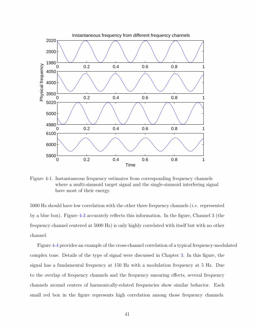
0 0.2 0.4 0.6 0.8 11980
2000
2020Instantaneous frequency from different frequency channels
0 0.2 0.4 0.6 0.8 13950
4000
4050
Phy
sica
l fre
quen
cy
0 0.2 0.4 0.6 0.8 14980
5000
5020
0 0.2 0.4 0.6 0.8 15900
6000
6100
Time
Figure 4-1. Instantaneous frequency estimates from corresponding frequency channelswhere a multi-sinusoid target signal and the single-sinusoid interfering signalhave most of their energy.
5000 Hz should have low correlation with the other three frequency channels (i.e. represented
by a blue box). Figure 4-3 accurately reflects this information. In the figure, Channel 3 (the
frequency channel centered at 5000 Hz) is only highly correlated with itself but with no other
channel.
Figure 4-4 provides an example of the cross-channel correlation of a typical frequency-modulated
complex tone. Details of the type of signal were discussed in Chapter 3. In this figure, the
signal has a fundamental frequency at 150 Hz with a modulation frequency at 5 Hz. Due
to the overlap of frequency channels and the frequency smearing effects, several frequency
channels around centers of harmonically-related frequencies show similar behavior. Each
small red box in the figure represents high correlation among those frequency channels.
41

Time
Fre
quen
cySpectrogram of the combined signal
0 0.1 0.2 0.3 0.4 0.5 0.6 0.7 0.8 0.90
1000
2000
3000
4000
5000
6000
7000
8000
Figure 4-2. Spectrogram of the signal described in Equation 4.3.
Figure 4-4 clearly shows that all the red boxes (“pixels”) are concentrated at frequencies
which are multiple integers of the fundamental frequency of 150 Hz. In the figure the first
and second blue lines represent the first and second harmonics at 150 Hz and 300 Hz,
respectively.
Figure 4-5 shows the two-dimensional symmetric correlation matrix R from a real speech
segment where the dominant fundamental frequency is around 135.5 Hz. For any particular
frequency index k in a given correlation matrix R, a row vector (or equivalently a column
vector due to symmetry) represents every correlation values of this particular frequency bin
K with respect to the other frequency bins. It is reasonable to assume that those frequency
bins with harmonic structure should be highly correlated with each other, thus providing a
42

Frequency
Fre
quen
cyCross−channel correlation of tested signal
0 1000 2000 5000 60000
1000
2000
5000
6000
Figure 4-3. Cross-channel correlation of four frequency channels where a multi-sinusoidtarget signal and single-sinusoid interfering signal have most of their energy.
relatively high average value if all correlation values for a given k are averaged. Equation
4.6 below describes how to calculate the average correlation value for each frequency bin.
RM(k) =1
K
K∑m=1
R(k,m) (4.6)
where, k and m are frequency bin indices, K is the total number of frequency bins, which are
typically the positive frequencies of the FFT that is evaluated in the STFT computation.
Once the average correlation is obtained, an empirically-derived threshold can be applied
to determine which frequency bins have an average correlation value that exceeds the threshold
and thus can be assumed to be correlated. We have observed empirically that a weak
43

Frequency
Fre
quen
cyCross−channel correlation of a Chowning signal at fundamental frequency of 150 Hz
200 400 600 800 1000 1200 1400 1600 1800 2000
200
400
600
800
1000
1200
1400
1600
1800
2000
150 Hz 300 Hz
Figure 4-4. Cross-channel correlation of a typical frequency-modulated complex tone at thefundamental frequency of 150 Hz.
speaker’s harmonic correlations do not have any impact as long as the local SNR is not too
close to zero (which is usually satisfied).
4.1.2 Mean Square Difference Mask Generation
Cross-channel correlation has already been demonstrated to be able to identify correlated
frequency components with common instantaneous frequency changes. Nevertheless, there
is an issue which may cause possible errors in grouping the frequency components. From the
theory discussed in Chapter 3, it is known that while the modulation frequency value itself
remains the same within a given harmonic structure with the same fundamental frequency,
the frequency deviation value is proportional to the order of the harmonics. In other
words, with a larger harmonic number, a larger frequency deviation will be observed. If
44

Frequency
Fre
quen
cyCross−channel correlation for a short voiced segment
500 1000 1500 2000 2500 3000 3500 4000
500
1000
1500
2000
2500
3000
3500
4000
Figure 4-5. Cross-channel correlation over all frequency bins for a short voiced segmentwith fundamental frequency 135.5 Hz. The red and yellow regions representhigh correlation, while blue and green regions represent low correlation.
different harmonics reflect the same modulation, then their actual frequency deviation will
be proportional to their harmonic numbers, so they will correlate with one another, but not
be equal. The problem with correlation is that it can lead to spurious matches between
components whose changes are proportional, but not in the appropriate scale (e.g. a high
frequency with a slightly positive trend in instantaneous frequency can correlate strongly
with a lower frequency with a much larger instantaneous frequency trend that happens to
be linear and positive as well).
In addition to applying correlation, other methods such as mean-squared difference
(MSD) can be used to provide further pruning of those frequency channels which are picked
up mistakenly. This combined method will be more reliable.
45

We make use of the signal described in Equations 4.5 and 4.3 to demonstrate this case,
but with a different interfering signal. Specifically, the frequency deviation is changed to 10
Hz as in Equation 4.7 to test whether MSD can detect and further prune it out from the
selection of cross-channel correlation.
θ1(t) = 2πfc1t +10
fm
sin(2πfmt) (4.7)
Table 4-1 shows the correlation values obtained using the cross-correlation method, where
the ground truth is that frequency channel 3 should not be included in the final selection.
As it is, frequency channel 3 demonstrates as a high correlation value in Table 4-1, as
do all other frequency channels, which results in a failure to exclude Channel 3 from the
frequency-component grouping. The reason is simply because the correlation calculation
rules out consideration of a proportional increase of deviation frequency as discussed above.
freq1 freq2 freq3 freq4freq1 1 1 1 0.997freq2 1 1 1 0.998freq3 1 1 1 0.997freq4 0.997 0.998 0.997 1
Table 4-1. Correlation using the cross-channel correlation method.
To solve this problem, Equation 4.8 is used to calculate the Mean Square Difference
(MSD). Using this method, the distance between frequency channels from the same harmonic
structures should have smaller values than those between the other channels.
MSD(k0, k1) =1
M
M∑m=1
(ω(m, k0)− ω(m, k0)
ω(m, k0)− ω(m, k1 − ω(m, k1)
ω(m, k1))2 (4.8)
where ω(m, k0) and ω(m, k1) represent the instantaneous frequencies from channel k0 and k1
at time index m and M is the total number of frames included in the calculation.
Table 4-2 illustrates results calculated using the MSD method and applied to the same
signal, where the difference between channel 1 and channel 3 is abnormally high. Table 4-1
first provides a set of frequency channels that are believed to come from the same source.
46

Table 4-2 is used to further remove the spurious channels. Combining Table 4-2 with Table
4-1, the desired final result can be achieved.
freq1 freq2 freq3 freq4freq1 0 0 0.3103 0.0003freq2 0 0 0.3120 0.0002freq3 0.3103 0.3120 0 0.3154freq4 0.0003 0.0002 0.3154 0
Table 4-2. Instantaneous frequency distance using the mean square difference method.
4.2 One-Dimensional Projection Solution
Both cross-channel correlation and mean square difference provide a two-dimensional
representation of the relationships among all frequency channels. Nevertheless, the best way
to project this two-dimensional information into one dimension and obtain the corresponding
frequency index remains unclear. There are many ways to extract this information. One
straightforward idea is to take the sum or average across each frequency index (e.g. across
each row or column in Figure 4-3, 4-4). Since the correlation matrix is symmetric, the sum
or average could be calculated across either the rows or columns.
Equation 4.6 shows how the one-dimensional projection is calculated. By averaging over
the columns of R(k,m) we obtain the average correlation for each row or column.
The frequency channels, which are members of the harmonic structure corresponding
to the fundamental frequency, usually have high correlation values with other frequency
channels also belong to the same harmonic structure. If one channel does not share a
common modulation frequency with the others, it is rare to observe high correlation values
with other frequency channels. Therefore, for the final one-dimensional average across the
frequency index, it is reasonable to see that the members of the harmonic structure generally
have high average correlation values, while other frequencies have relatively low values.
Figure 4-6 demonstrates the simplest case of the application of one-dimensional projection
where the signal described in Equation 4.3 is used. In this case, it is already known from
ground truth that the third frequency channel analyzed does not come from the same
47
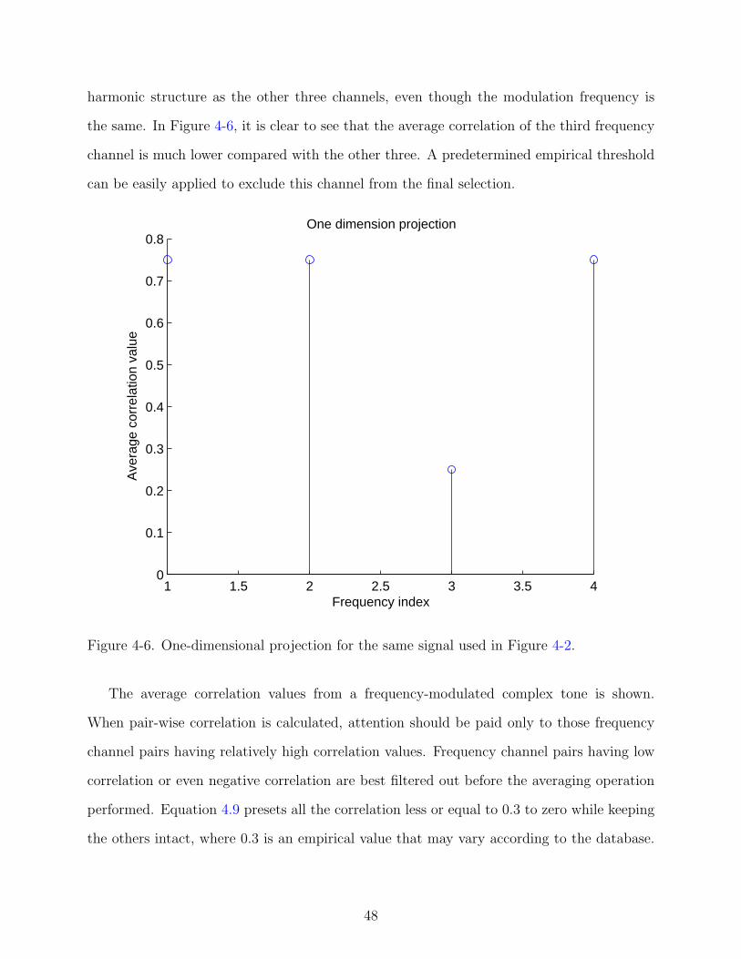
harmonic structure as the other three channels, even though the modulation frequency is
the same. In Figure 4-6, it is clear to see that the average correlation of the third frequency
channel is much lower compared with the other three. A predetermined empirical threshold
can be easily applied to exclude this channel from the final selection.
1 1.5 2 2.5 3 3.5 40
0.1
0.2
0.3
0.4
0.5
0.6
0.7
0.8
Frequency index
Ave
rage
cor
rela
tion
valu
e
One dimension projection
Figure 4-6. One-dimensional projection for the same signal used in Figure 4-2.
The average correlation values from a frequency-modulated complex tone is shown.
When pair-wise correlation is calculated, attention should be paid only to those frequency
channel pairs having relatively high correlation values. Frequency channel pairs having low
correlation or even negative correlation are best filtered out before the averaging operation
performed. Equation 4.9 presets all the correlation less or equal to 0.3 to zero while keeping
the others intact, where 0.3 is an empirical value that may vary according to the database.
48
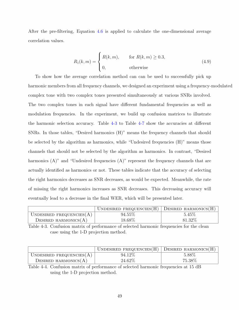
After the pre-filtering, Equation 4.6 is applied to calculate the one-dimensional average
correlation values.
R1(k, m) =
R(k,m), for R(k, m) ≥ 0.3,
0, otherwise
(4.9)
To show how the average correlation method can can be used to successfully pick up
harmonic members from all frequency channels, we designed an experiment using a frequency-modulated
complex tone with two complex tones presented simultaneously at various SNRs involved.
The two complex tones in each signal have different fundamental frequencies as well as
modulation frequencies. In the experiment, we build up confusion matrices to illustrate
the harmonic selection accuracy. Table 4-3 to Table 4-7 show the accuracies at different
SNRs. In those tables, “Desired harmonics (H)” means the frequency channels that should
be selected by the algorithm as harmonics, while “Undesired frequencies (H)” means those
channels that should not be selected by the algorithm as harmonics. In contrast, “Desired
harmonics (A)” and “Undesired frequencies (A)” represent the frequency channels that are
actually identified as harmonics or not. These tables indicate that the accuracy of selecting
the right harmonics decreases as SNR decreases, as would be expected. Meanwhile, the rate
of missing the right harmonics increases as SNR decreases. This decreasing accuracy will
eventually lead to a decrease in the final WER, which will be presented later.
Undesired frequencies(H) Desired harmonics(H)Undesired frequencies(A) 94.55% 5.45%
Desired harmonics(A) 18.68% 81.32%
Table 4-3. Confusion matrix of performance of selected harmonic frequencies for the cleancase using the 1-D projection method.
Undesired frequencies(H) Desired harmonics(H)Undesired frequencies(A) 94.12% 5.88%
Desired harmonics(A) 24.62% 75.38%
Table 4-4. Confusion matrix of performance of selected harmonic frequencies at 15 dBusing the 1-D projection method.
49

Undesired frequencies(H) Desired harmonics(H)Undesired frequencies(A) 97.06% 2.94%
Desired harmonics(A) 26.15% 73.85%
Table 4-5. Confusion matrix of performance of selected harmonic frequencies at 10 dBusing the 1-D projection method.
Undesired frequencies(H) Desired harmonics(H)Undesired frequencies(A) 97.06% 2.94%
Desired harmonics(A) 38.46% 61.54%
Table 4-6. Confusion matrix of performance of selected harmonic frequencies at 5 dB usingthe 1-D projection method.
4.3 Graph-Cut Solution
Currently simple average correlation approach discussed in the previous section has been
used to find highly-correlated frequency bins, by simple averaging along one dimension to
reduce the two-dimensional correlation matrix to one dimension with modest computation.
While this approach is attractive because of its low computation load, straightforward
physical meaning, and relatively easy implementation, it does not exploit the structure of the
correlation matrix itself. Image segmentation and grouping have provided many promising
directions toward better solutions of this problem. The idea in image segmentation is to
minimize the distance between members from the same group while maximizing the distance
between members from different groups, which is quite similar to linear discriminant analysis
(LDA) [17]. Among several graph-cut algorithms, Shi and Malik’s work [43] provides a good
entry point to explore the correlation and improve the final performance.
Rather than focusing on local features and their consistencies in the two-dimensional
correlation representation, the graph-cut approach aims at extracting the global impression
of the 2D image. Image segmentation is treated as a graph partitioning problem. The
Undesired frequencies(H) Desired harmonics(H)Undesired frequencies(A) 77.94% 22.06%
Desired harmonics(A) 33.85% 66.15%
Table 4-7. Confusion matrix of performance of selected harmonic frequencies at 0 dB usingthe 1-D projection method.
50

graph-cut criterion measures both the total dissimilarity between the different groups as well
as the total similarity within the groups. In this way, the problem of how to efficiently extract
the pattern contained in the 2D correlation matrix can be transferred into an eigenvalue and
eigenvector problem, where the correlation can be the target matrix to be solved.
This approach is most related to the graph theoretic formulation of grouping. The set of
points in an arbitrary feature space is represented as a weighted undirected graph G = (V, E),
where the nodes of the graph are the points in the feature space (a set V ), and an edge is
formed between every pair of nodes (a set E). The weight on each edge, w(i, j), is a function
of the similarity between nodes i and j.
In grouping, the goal is to seek to partition the set of vertices into disjoint sets V1; V2;
· · · ; Vm, where by some measure the similarity among the vertices in a set Vi is high and,
across different sets Vi, Vj is low.
Figure 4-7 shows an undirected graph G, which has 9 nodes. The index of each node
is marked in red and the correlation between each node is represented in black. From the
figure, it is easy to see that the entire graph can be divided into two sub-graphs, where
Nodes 1, 2, 3 and 4 fall into one sub-graph and Nodes 5 to 9 belong to the other graph.
All the nodes can be considered as an n-dimensional feature vector. The undirected graph
is sitting in the same n-dimensional space. There are multiple ways to calculate the values
between each node. Euclidean distance and other distance measures can be used, where the
closer two nodes are, the smaller values are. In Figure 4-7, all values shown in the figure are
correlation, where the closer two nodes are, the larger values are.
Equation 4.10 below is a matrix representation of the graph shown in Figure 4-7. The
matrix is also called affinity matrix, which will be discussed in detail. Suppose there is
a binary weight vector w (which is also called an indicator vector) with length equal to
the number of nodes in the entire graph G, where each of its component is 1 when the
corresponding node is sitting in a desired sub-graph C, as in Equation 4.11. Equation 4.12
can be used to calculate the average association between all nodes in the same sub-graph
51
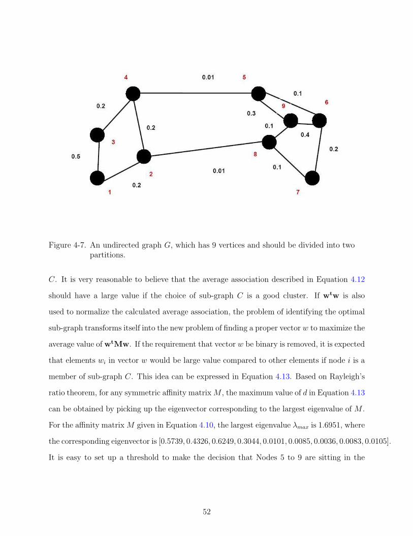
Figure 4-7. An undirected graph G, which has 9 vertices and should be divided into twopartitions.
C. It is very reasonable to believe that the average association described in Equation 4.12
should have a large value if the choice of sub-graph C is a good cluster. If wtw is also
used to normalize the calculated average association, the problem of identifying the optimal
sub-graph transforms itself into the new problem of finding a proper vector w to maximize the
average value of wtMw. If the requirement that vector w be binary is removed, it is expected
that elements wi in vector w would be large value compared to other elements if node i is a
member of sub-graph C. This idea can be expressed in Equation 4.13. Based on Rayleigh’s
ratio theorem, for any symmetric affinity matrix M , the maximum value of d in Equation 4.13
can be obtained by picking up the eigenvector corresponding to the largest eigenvalue of M .
For the affinity matrix M given in Equation 4.10, the largest eigenvalue λmax is 1.6951, where
the corresponding eigenvector is [0.5739, 0.4326, 0.6249, 0.3044, 0.0101, 0.0085, 0.0036, 0.0083, 0.0105].
It is easy to set up a threshold to make the decision that Nodes 5 to 9 are sitting in the
52

sub-graph C, which also automatically places Nodes 1 to 4 in the other sub-graph if the
assumption is that there are only two sub-graphs.
R =
1 0.2 0.5 0 0 0 0 0 0
0.2 1 0.2 0.2 0 0 0 0.01 0
0.5 0.2 1 0.2 0 0 0 0 0
0 0.2 0.2 1 0.01 0 0 0 0
0 0 0 0.01 1 0.1 0 0 0.3
0 0 0 0 0.1 1 0.2 0 0.4
0 0 0 0 0 0.2 1 0.1 0
0 0.1 0 0 0 0 0.1 1 0.1
0 0 0 0 0.3 0.4 0 0.1 1
(4.10)
wi =
1, if i ∈ C,
0, otherwise
(4.11)
wtRw =∑i,j∈C
mij (4.12)
d = MaxwtRw
wtw(4.13)
Undesired frequencies(H) Desired harmonics(H)Undesired frequencies(A) 95.28% 4.72%
Desired harmonics(A) 13.14% 87.86%
Table 4-8. Confusion matrix of performance of selected harmonic frequencies for the cleancase by using the graph-cut method.
Undesired frequencies(H) Desired harmonics(H)Undesired frequencies(A) 94.97% 5.03%
Desired harmonics(A) 19.77% 80.23%
Table 4-9. Confusion matrix of performance of selected harmonic frequencies at 15 dB byusing the graph-cut method.
53

Though both one-dimensional projection and the graph-cut approach provide good ability
to identify a correlation pattern from its 2-D representation in theory, the later demonstrates
superior performance compared to the former. In Equation 4.13, the vector w is able to
iterate all possibilities of cutting the 2-D correlation into different sub-graphs by changing
each individual element inside w. The best existing vector w is the eigenvector corresponding
to the largest eigenvalue of the correlation matrix R.
Undesired frequencies(H) Desired harmonics(H)Undesired frequencies(A) 97.79% 2.21%
Desired harmonics(A) 20.28% 79.72%
Table 4-10. Confusion matrix of performance of selected harmonic frequencies at 10 dB byusing the graph-cut method.
Figure 4-8 and Figure 4-9 illustrate the superiority of using the graph-cut method compared
to one-dimensional projection by plotting the selection results using the two methods.
Table 4-8 to Table 4-12 show the performance with confusion matrices by applying the
graph-cut method to the same signals described above. The results reconfirm that the
graph-cut method is more reliable than one-dimension projection with a penalty of a greater
computational load in calculating eigenvalues and eigenvectors for each correlation matrix.
We will compare these two methods in terms of their impact on speech recognition accuracy
in the following chapter.
Undesired frequencies(H) Desired harmonics(H)Undesired frequencies(A) 96.36% 3.64%
Desired harmonics(A) 30.77% 69.23%
Table 4-11. Confusion matrix of performance of selected harmonic frequencies at 5 dB byusing graph-cut method.
Undesired frequencies(H) Desired harmonics(H)Undesired frequencies(A) 76.47% 23.53%
Desired harmonics(A) 32.31% 67.69%
Table 4-12. Confusion matrix of performance of selected harmonic frequencies at 0 dB byusing graph-cut method.
54
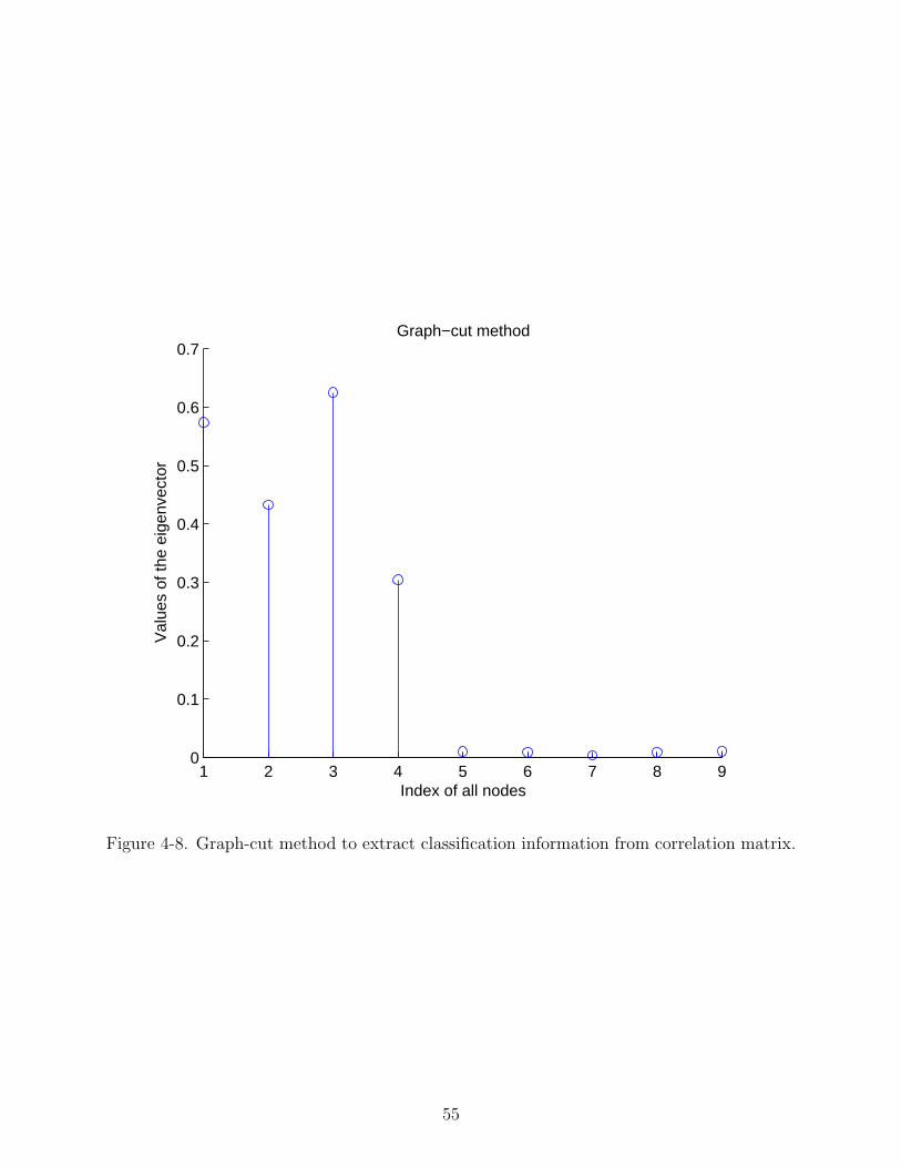
1 2 3 4 5 6 7 8 90
0.1
0.2
0.3
0.4
0.5
0.6
0.7
Index of all nodes
Val
ues
of th
e ei
genv
ecto
r
Graph−cut method
Figure 4-8. Graph-cut method to extract classification information from correlation matrix.
55

1 2 3 4 5 6 7 8 90
0.05
0.1
0.15
0.2
0.25
Index of all nodes
Ave
rage
d va
lues
from
the
corr
elat
ion
mat
rix
One−dimension projection method
Figure 4-9. 1-D projection method to extract classification information from correlationmatrix.
56
CHAPTER 5GROUPING SCHEMES AND EXPERIMENTAL DESIGN
In the previous chapters we have discussed the estimation of instantaneous frequency, the
application of cross-channel correlation and the utilization of graph-cut theory to identify
frequency channels from the same speech source.
In this chapter, the solution of how to regroup frequency components identified from
the same source will be discussed, which includes pitch detection and traditional speaker
identification. In addition, a sieve function will be introduced to refine further the selected
harmonic structure obtained from the cross-channel correlation function based on instantaneous
frequency. A general discussion about the generation of binary masks will follow. Finally,
experimental results will be presented that compare our proposed algorithm with several
others, including baseline Mel-Frequency Cepstral Coefficients (MFCC), a multi-pitch tracking
algorithm and an instantaneous-amplitude-based algorithm.
5.1 Grouping Schemes
As mentioned above, there are two major stages in speech separation, segregation and
regrouping. Chapters 3 and 4 include a detailed discussion of how to use instantaneous-
frequency-based cross-channel correlation to achieve segregation. In real experiments, this
stage simply makes a decision about how many frequency channels are believed to have the
same harmonic structure in each processed frame.
Nevertheless, this is not the end of the story. In order to reconstruct the entire utterance,
we usually must determine whether the clustered frequency channels from the first stage
in each individual frame are from the target speaker or from a competing speaker. This
challenge introduces the second important stage in speech separation, regrouping.
In general, the evaluation of systems that separate two speakers is typically divided into
two categories: the same-gender and different-gender cases. In this chapter we will describe
two different schemes that address this problem, which are based on pitch detection for the
different-gender case and speaker identification for the same-gender and the general cases.
57

5.1.1 Pitch Detection for Dominant Speakers for the Different-Gender Case
Pitch detection for grouping of speakers can be used for the different-gender case only,
when it is known a priori that the target and masking speakers are of the opposite gender.
The speech of speakers of different genders have fundamental frequencies that seldom overlap
and that frequently are quite far from one another. The harmonic structures from the target
speaker and interfering speaker are not very likely to overlap as well.
When the SNR is greater than zero, even though the interfering speaker might be the
dominant speaker in some frames, the majority of the frames are likely to represent the
pitch contour of the target speaker. After a simple pitch estimation, it is relatively easy
to determine the pitch range of the target speaker, as a single pitch contour most likely
represents the pitch from the dominant speaker from each individual frame. If the majority
of the pitch contours is below approximately 160 Hz, there is a high chance that the dominant
speaker of the entire utterance is a male speaker. Based on similar logic, a female dominant
speaker is easy to detect if the majority of the pitch frames is above 160 Hz.
After applying the instantaneous-frequency-based cross-channel correlation for each individual
frame, all frequency channels are classified into two groups, one associated with the dominant
speaker and the other with the interfering speaker. Frames are sorted according to whether
the dominant speaker is assumed to be the target or interfering speaker based on this pitch
information.
Two comments are worth noting here. First, the pitch estimation described here is
not the multi-pitch algorithm mentioned in previous chapters that provides separate pitch
contours for the target and interfering speakers. This pitch extraction is nothing more than
a very simple conventional pitch estimator that attempts to determine only the pitch of
the dominant speaker in each frame, which may not be the target speaker. In addition,
the resolution requirement for pitch estimation is very loose, as it is only necessary that
the system be able to discriminate between the target and interfering speaker. The task
58

of determining which frequency channel belongs to target and interferor is handled by the
instantaneous-frequency-based cross-channel correlation.
We remind the reader that the pitch-detection approach can work only for the different-gender
scenario, as noted above. On the other hand, the pitch-detection method does not require
any historical data or a priori information, which is needed for the speaker-identification
method introduced below.
Figure 5-1 is a block diagram of a speech separation system that uses pitch detection to
regroup cluster frequency components from each individual frame to reconstruct the speech.
In the diagram, the simultaneous speech is first processed by two parallel processes. The
upper panel implements the STFT, performs instantaneous frequency estimation, cross-channel
correlation algorithm to cluster frequency components believed to be from the dominant
speaker. In the lower panel, pitch estimation is performed in the time domain to obtain a
rough estimate of whether the current processed frame is from the target or the interfering
speaker. If a processed frame is believed from the target speaker, the clustered frequency
components from that frame are selected to contribute to the final output speech. If a frame
is from the interfering speaker, on the other hand, the frequency channels associated with it
are suppressed instead.
5.1.2 Speaker Identification for the Same-Gender Case
Speaker identification is widely used as another way to detect the dominant speaker and
use that information to accomplish further regrouping. The key idea here is each speaker has
his or her own characteristics that can be identified using conventional speaker identification
(SID) technology. These results are used as the basis to identify the dominant speakers
associated with each input frame, assuming that the speakers to be separated are one of a
number contained in the training data.
In a typical SID system, there is a certain amount of training data provided for each
speaker. MFCC coefficients are typically used as the features and Gaussian mixture model
59

Figure 5-1. Block diagram of a system that uses pitch detection to determine the dominantspeaker.
(GMMs) are used to characterize each speaker. A the parameter set λ that characterizes
each speaker consists of p, ~µ and Σ:
λ = {pi, ~µi, Σi}, i = 1, 2, . . . , M (5.1)
where p is the a prioi probability of each Gaussian mixture, ~µ is the MFCC mean vector, Σ is
the covariance for each Gaussian component and M is the number of Gaussian components
used. These three parameters can be estimated by maximum likelihood estimation [38].
The probablity density for each component is a multi-variate Gaussian:
bi(~x) =1
(2π)D/2|∑i |1/2exp{−1
2(~x− ~µi)
T Σ−1i (~x− ~µi)} (5.2)
The final Gaussian mixture density is easily obtained according to the equation:
p(~x|λ) =M∑i=1
pibi(~x) (5.3)
Using the formulation above, the SID system calculates a posteriori probability for each
speaker according to the equation:
60
p(k|~x, λk) =gkbk(~x)∑Kk=1 gkbk(~x)
(5.4)
If there is a total K speakers and the priori for each speaker is gk, the dominant speaker is
dominant is determined to be the speaker with vector or observation sequence which contains
the largest p(k|~x, λk).
For simultaneously-presented speech, the dominant speaker is identified on a frame-by-frame
basis, and either of the methods described in the previous chapter is used to determine which
frequency bins in that frame belong to that speaker, as in the previous section.
While this method can be used for both same-gender and different-gender scenarios, it
does require a priori information for each speaker. It will not work properly for speakers
that are not known previously to the system.
Figure 5-2 is a block diagram of a system that use speakers identification to identify
the dominant speaker and further regroup speech stream. The only difference between this
figure and Figure 5-1 is the bottom branch, in which the identity of the dominant speaker
for the current frame is determined based on previously-compiled statistical information.
5.2 Mask Generation
In Section 4, we discussed how to obtain a binary mask based on the spectrogram for
every utterance processed. The general idea is to use cross-channel correlation classification
based on instantaneous frequency to select frequency channels that are highly correlated with
the same harmonic structure. While constructing the binary mask, those time-frequency
cells that are believed to belong to the same harmonic structure as the dominant speaker
are assigned a value of 1. All other cells are assigned a value of 0. The target speech is
reconstructed using only those cells with a value of 1 are used, while the other cells with a
mask value of 0 are suppressed.
In order to utilize the advantages of the short-time Fourier transform to track the
changes in instantaneous frequency, while still analyzing features over a longer time period
for separation purposes, each utterance is divided into multiple frames of duration 75 ms.
61

Figure 5-2. Block diagram of a speech separation system that uses speaker identification todetermine the dominant speaker.
Each of these frames are overlapped by 25 or 50 percent of the frame length, depending on
the application. The cross-channel correlation classification is applied within each frame to
generate the binary mask.
One issue with this procedure is that multiple computations of the binary mask in each
frame are obtained because of the overlap of analysis frames. This is addressed by averaging
the values of the binary mask for a given frame over all of the analysis frames that include
that frame. The components of this averaged mask are then compared to a pre-determined
threshold:
M1(n, k) =1
n1 − n0 + 1
n1∑n=n0
M(n, k) (5.5)
62

M2(n, k) =
1, if M1(n, k) ≥ thresh,
0, otherwise
(5.6)
where M(n, k) is the original binary mask, n and k are the frame and frequency bin index,
respectively. Alternatively, in many applications the averaged M1(n, k) can also be used
directly and conversion into the binary mask M2(n, k) is not necessary.
5.3 Experimental Procedures and Databases
5.3.1 Sphinx-III Recognition Platform
We use the Sphinx open-source automatic speech recognizer developed at Carnegie Mellon
University, one of the first systems to demonstrate speaker-independent, large vocabulary
continuous speech recognition (LVCSR). The original Sphinx-I system was developed by
Kai-Fu Lee in 1988, and Sphinx was extended by many individuals in later versions. Current
versions of Sphinx are implemented in C and in Java, and there is also a version of the code
that is optimized for embedded systems with a small footprint.
We make use of Sphinx-III in our work as it provides flexibility in modeling and feature
development for speech recognition. As in the case of most other large vocabulary continuous
speech recognition (LVCSR) systems, Sphinx-III is a phoneme-based system, with each
phoneme modeled by an HMM. Word-level HMMs are obtained by concatenating associated
phonemes together using triphone context-dependent acoustic models. HMMs states are
modeled in the usual left-to-right fashion. Due to the large number of model parameters, the
parameters of the Gaussian distribution characterizing each state can be shared by different
states. In addition, states can be pruned or combined to reduce the number of parameters.
Figure 5-3 [31] is a block diagram of the Sphinx-III recognition system.
5.3.2 The Resource Management and Grid Corpora
Two standard speech corpora were used to evaluate the various source separation algorithms
considered: the Grid database which had been used in the Speech Separation Challenge of
2006 [11, 12] and the familiar DARPA Resource Management (RM) database [35]. The Grid
63

Figure 5-3. A block diagram of the Sphinx-III speech recognition system.
database is a large multitalker audiovisual sentence corpus to support behavioral studies
in speech perception. In brief, the corpus consists of high-quality audio and video (facial)
recordings of 1000 sentences spoken by each of 34 talkers (18 male, 16 female). All speech
files are single-channel “wav” data sampled at 25 kHz and all material is endpointed. The
corpus, together with transcriptions, is freely available for research use [11]. The Grid
training corpus includes 34 speakers, each providing 500 clean utterances, for a total of
64

17,000 clean training utterances. The testing utterances are degraded at various SNRs, and
each condition contains 600 sentences. All utterances in the Grid database have a fixed
format as specified in Table 5-1. Specifically, each sentence contains six words, starting with
a command, following by a color, a preposition, a letter, a number and finally an adverb.
The database contains 4 command words, 4 colors, 4 prepositions, 25 letters, 10 numbers,
and 4 adverbs [13]. For example, a typical sentence could be “Bin white at D 1 again”. We
used only the speech with an SNR of +6 dB in the present work.
The DARPA Resource Management Continuous Speech Corpora (RM) [35] consists of
digitized and transcribed speech for use in designing and evaluating continuous speech
recognition systems. All RM material consists of read sentences modeled after a Naval
resource management task. The complete corpus contains over 25,000 utterances from
more than 160 speakers representing a variety of American dialects. The material was
recorded at 16 kHz, with 16-bit resolution, using a Sennheiser HMD-414 headset microphone.
Speaker-Independent training and testing data are used for this dissertation. This part of
the DARPA RM database consists of 1600 training utterances and 600 testing utterances.
The vocabulary size of RM database is nominally 1000 words and was purposefully made to
be phonetically balanced.
verb color preposition letter digit adverbbin blue at A–Z 1-9 againlay green by (no ‘W’) and zero now
place red on pleaseset white with soon
Table 5-1. Structure of the sentences in the Grid database.
The evaluation methods used for the two corpora are quite different. As noted above,
sentences in the Grid database all consist of a verb followed by a color, a preposition, a
letter, a digit, and an adverb in precisely that sequence. The task is to recognize the digit
and letter in the sentence which contains the color “white”. The only errors tabulated are
substitutions for the digits and letters in the speech data due to their fixed positions. The
task remains a difficult one, as digits and letters are frequently confused even by human
65
listeners when competing speakers are present. We used the scoring tool prepared by the
University of Sheffield to score recognition results for the Grid database. As discussed in the
previous section, speaker identification is used to regroup speech streams in the same-gender
and general cases. In contrast, the task in Resource Management database is simply to
recognize each testing sentence and the word error rate (WER) is tabulated. The WER is
by definition the number of substitution, insertion, and deletion errors divided by the total
number of words presented. Pitch detection is generally used to group the components of
the final reconstructed speech stream.
5.4 Experimental Results and Discussion
This section describes various experimental results obtained for the algorithms described
above using data from the RM and Grid databases.
In Chapter 4, we argued that the graph-cut approach is a good way to cluster the
frequency components that are obtained from clustering information from the correlation
matrix. Figure 5-4 below demonstrates that the graph-cut method is more effective in
extracting correlation information than the 1-D projection method, and thus results in better
recognition accuracy. These results were obtained using the RM database. We used the NIST
tool sc stats to test statistical significance between different algorithms. The differences
between the two methods are all statistically significant at the level of p < .05 except for the
clean case. The system shown in Figure 5-1 was used to extract features and reconstruct
speech. The results are tested on the RM database for the different gender-case.
We also compared the performance of the cross-channel correlation algorithm based on
instantaneous frequency that was developed in this thesis to other well known approaches.
Figure 5-1 compares results using our approach to similar results obtained using baseline
Mel-Frequency Cepstral Coefficients (MFCC), the multi-pitch tracking algorithm developed
by de Cheveigne, and an algorithm based on instantaneous amplitude estimation.
The fundamental idea of the multi-pitch tracking algorithm is to estimate different
fundamental frequencies one by one. The fundamental frequency from the dominant speaker
66
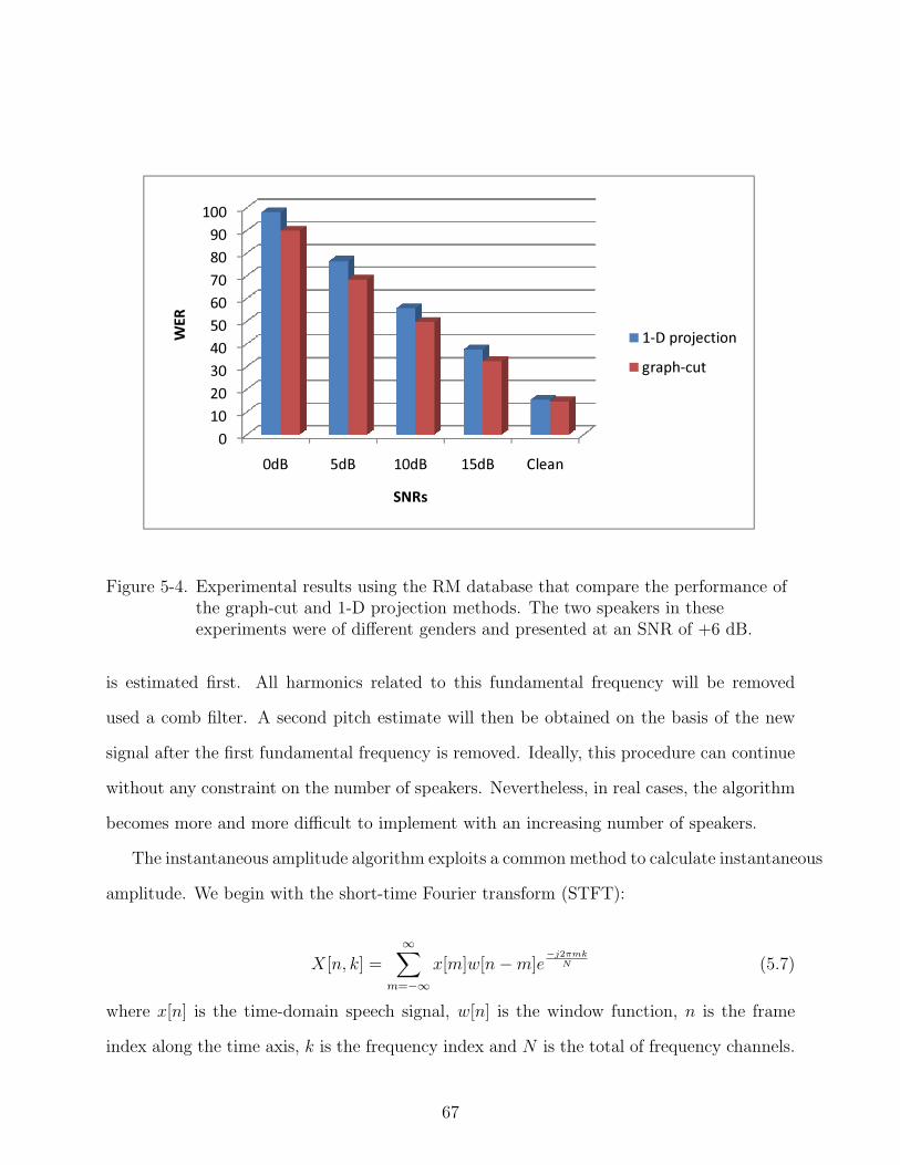
��������������������
��� ��� ���� ���� ����
���
����
�����������������������
Figure 5-4. Experimental results using the RM database that compare the performance ofthe graph-cut and 1-D projection methods. The two speakers in theseexperiments were of different genders and presented at an SNR of +6 dB.
is estimated first. All harmonics related to this fundamental frequency will be removed
used a comb filter. A second pitch estimate will then be obtained on the basis of the new
signal after the first fundamental frequency is removed. Ideally, this procedure can continue
without any constraint on the number of speakers. Nevertheless, in real cases, the algorithm
becomes more and more difficult to implement with an increasing number of speakers.
The instantaneous amplitude algorithm exploits a common method to calculate instantaneous
amplitude. We begin with the short-time Fourier transform (STFT):
X[n, k] =∞∑
m=−∞x[m]w[n−m]e
−j2πmkN (5.7)
where x[n] is the time-domain speech signal, w[n] is the window function, n is the frame
index along the time axis, k is the frequency index and N is the total of frequency channels.
67
The square of the instantaneous amplitude is typically obtained from the sum of the
squares of the real and imaginary parts of X[n, k]:
E[n, k] = (<X[n, k])2 + (=X[n, k])2 (5.8)
where <(X[n, k]) is the real part of X[n, k] and =(X[n, k]) is the imaginary part of X[n, k].
Figure 5-5 compares the recognition accuracy obtained with the four procedures and
demonstrates that the instantaneous-frequency-based algorithm provides the best performance
of the four algorithms considered. Since the RM database tested here is for the different-gender
case, the regrouping scheme used here is based on pitch detection, as described in Figure
5-1.
While the multi-pitch tracking algorithm is helpful in our experiment, it does not provide
a large improvement in performance. The reasons is that the final extraction and suppression
of harmonic structure is highly dependent on the accuracy of pitch estimation. Any error
made in pitch estimation will adversely affect the final results. In fact estimating simultaneous
pitches of multiple signals is very challenging in and of itself.
Besides the instantaneous-frequency-based method, the instantaneous amplitude-based
method also shows good improvement. In contrast to the instantaneous-frequency-based
method, the change of instantaneous-amplitude movement is not very selective, which results
some frequency channels becoming mistakenly accepted due to false high correlation values.
In addition to that, “coherent demodulation” is also very important for the instantaneous-amplitude-based
method. Knowing exactly the carrier frequency of the test signal will greatly increase the
accuracy of “coherent demodulation”. However, this is also a challenging topic by itself.
Compared to the multi-pitch and instantaneous-amplitude-based algorithms, our instantaneous-frequency-based
algorithm does not require that the instantaneous frequency be estimated with high accuracy.
Even with interfering components present, the cross-channel correlation is still able to pick
up those frequency channels that are less affected by the interference. All these factors
68
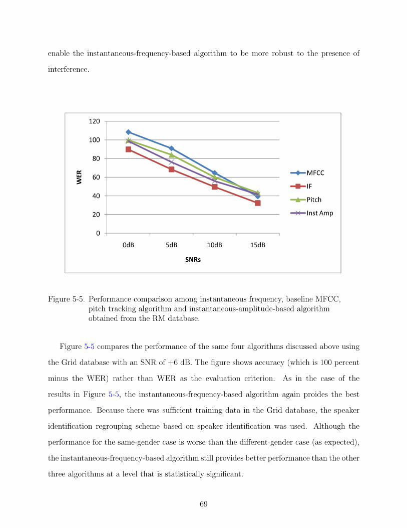
enable the instantaneous-frequency-based algorithm to be more robust to the presence of
interference.
�
��
��
��
��
���
���
��� �� ���� ���
���
����
��� ������ �������
Figure 5-5. Performance comparison among instantaneous frequency, baseline MFCC,pitch tracking algorithm and instantaneous-amplitude-based algorithmobtained from the RM database.
Figure 5-5 compares the performance of the same four algorithms discussed above using
the Grid database with an SNR of +6 dB. The figure shows accuracy (which is 100 percent
minus the WER) rather than WER as the evaluation criterion. As in the case of the
results in Figure 5-5, the instantaneous-frequency-based algorithm again proides the best
performance. Because there was sufficient training data in the Grid database, the speaker
identification regrouping scheme based on speaker identification was used. Although the
performance for the same-gender case is worse than the different-gender case (as expected),
the instantaneous-frequency-based algorithm still provides better performance than the other
three algorithms at a level that is statistically significant.
69

�
��
��
��
��
��
��
��� ����� ���������� ����� ������
��������
�����������������
Figure 5-6. Comparison of performance of the instantaneous frequency, baseline MFCC,pitch tracking, and instantaneous-amplitude-based algorithm using data fromthe Grid database.
One advantage of using the instantaneous-frequency-based cross-channel correlation algorithm
to separate speech is that it has the ability to filter out the parts of the harmonic structure
from the target speech that are affected by the interfering speaker. For example, if the
fundamental frequency of the target speaker is 150 Hz while the interfering speaker has a
fundamental frequency of 200 Hz, the fourth harmonic of the target speaker is identical
to the third harmonic of the interfering speaker, 600 Hz. In this case the instantaneous
frequency estimated at 600 Hz would be severely affected by the interfering speaker, the
instantaneous frequency estimated from this channel is unlikely to have a high correlation
with other components of the target speaker that are less affected by the components of the
interfering speaker. Thus this channel would be excluded from the final reconstruction.
70

Figure 5-7 shows the results of an experiment that was designed to illustrate this point
on RM database. First, we estimated the fundamental frequency and all related harmonics
for clean speech from a given speaker. Next we added interfering speech at various SNRs.
The target speech was reconstructed in two ways using the instantaneous-frequency-based
method: using a mask derived from the clean speech, which presumably contains all components
of the signal, and using a mask that was obtained automatically from the noisy speech,
which presumably excludes the components that were adversely affected by the presence of
the masker. The results in Figure 5-7 clearly show that the reconstructed speech obtained
from harmonics estimated from clean speech leads to worse recognition accuracy because
of the inclusion of frequency channels that are degraded by the presence of the masker. In
contrast, reconstructed speech from harmonics obtained directly from noisy speech yields
substantially better WER.
5.5 A Sieve Function for Selecting Relevant Frequency Components fromPartial Harmonic Structure
In previous chapters, frequency components believed to be from the same source were
identified and grouped together based on the proposed temporal features of instantaneous
frequency and the classification method used was that of cross-channel correlation. However,
due to the presence of competing speech, there are inevitable estimation errors from both
the procedure of estimating instantaneous frequency and of using the graph-cut algorithm to
group similar frequency components. These estimation errors adversely impact on the final
harmonic structure used to reconstruct speech, which eventually will limit the improvement
of the final WER.
5.5.1 Harmonic Pattern Recognition
In this section, a sieve function scheme is proposed to compensate for this problem
[44, 45]. This approach is based on the assumption that the components to be included are
all harmonically related to one another. A harmonic “sieve” is applied with a fundamental
frequency that is chosen to maximize the value of an objective cost function based on the
71

�
��
��
��
��
���
���
��� �� ���� ���
���
����
�� ��������������
�� �������������
Figure 5-7. Comparison of WER obtained using a reconstruction of masked speech usingall components of the dominant speaker (“clean mask”) with a similarreconstruction using only those components that are identified as undistortedby the instantaneous-frequency-based method (“real mask”).
input spectrum that is described below. Once the fundamental frequency is chosen in this
fashion, the new estimated fundamental frequency and its associated harmonic structure
will be used to further filter out those “noisy” frequency channels mistakenly selected in the
original frequency-selection procedure used.
Assume that there is a superset F containing a set of fundamental frequencies f ranging
from 80 Hz to 350 Hz. This frequency range includes most of the reasonable fundamental
frequencies without regard to gender or age. Within this range we define a set of potential
fundamental frequencies f that each have their own harmonic structure. These frequencies
f are generally linearly spaced in F , although they do not need to be.
72

Given a specific fundamental frequency of f , all harmonic members related to this
fundamental frequency can be represented as f = [f1 ± σ, 2f1 ± σ, · · · , nf1 ± σ], where
n is the total number of elements in the harmonic structure, σ is a small tolerance range
around each harmonic in the set.
It is easy to see that the superset of F is fixed given a fixed number of fundamental
frequencies f and small tolerance σ. If the fundamental frequency is time varying, the
superset F is a function of f .
In this and the previous chapters we discussed a system that attempts to extract the
important harmonic components of masked speech based on cross-channel correlation and
graph-cut grouping. We refer to the harmonic structure estimated by the system described
in this and the previous chapter as S, and this structure is estimated for real simultaneously
presented speech. The set S can be given as S = [s1, s2, · · · , sm], where m is the total
number of elements in the set S. It is worthwhile to point out that the length of each subset
f inside F is not necessarily the same as the length of set S.
The harmonic pattern recognition goal is to compare each set of f belonging to the
superset of F with the estimated harmonic structure set S. The final selection of f values
that are assumed to be relevant is based on a pre-designed objective cost function to select
the final winner f in the set of F based on the maximum or minimum in order to determine
the final fundamental frequency.
5.5.2 The Harmonic Sieve
In the previous section, the basic idea of harmonic pattern recognition was discussed.
In this section details about the harmonic sieve will be provided in order to complete the
picture of how to filter out harmonic outliers.
Returning to the set F and S given above, set F is nothing but a superset dependent on
each different fundamental frequency and its corresponding mesh. Every set of fundamental
frequency and its mesh comprises one harmonic sieve. Let us consider a set of F harmonic
sieves, in which the f th sieve (f = 0, 1, 2, . . . , F − 1) has a fundamental frequency S[y] and
73
L meshes at harmonic frequencies f [y, h] = hS[y], h = 1, 2,. . . , L, where h is the number
of harmonics. The range of S[y] should be able to cover a reasonable range that contains
most of the possible fundamental frequencies. In this dissertation, we use the range from
80 Hz to 350 Hz. For the meshes introduced above, instead of setting a fixed mesh for each
harmonic frequency, we use a variable mesh, where each harmonic frequency f [y, h] has a
relative bandwidth of 2b. For instance, for a given harmonic f [y, h], the mesh begins from
the most left of (1− b)f [y, h] and extends itself to the most right of (1+ b)f [y, h]. The value
b is not necessarily a fixed value. In the experiments, we chose the value b from 10 to 15.
Now in reality, we have two different sets of frequencies. One is set F , which contains each
mesh set f [y, h] depending on the specific fundamental frequency y and order of harmonics
h. The other is set S, which is obtained from the cross-channel correlation identification.
Our goal is to use set F to further smooth set S and remove those outliers contained in
set S. By shifting or changing the values of f [y, h] while fixing the bandwidth b, only a
certain number of elements in set S can remain. The others, which do not fall into any of
the predesigned meshes, will be removed from the set.
5.5.3 Objective Function
An objective function is needed to compare among all possible sieve sets and determine
the final optimal pitch and its harmonics.
The first step is to assign a proper value to a certain mesh if there is at least one value
from set S falling into it. Let’s assume each element in set S is represented as s[i]. The
following equation shows how to label each mesh:
r[y, i] =
h, if (1− b)f [y, h] < x[i] < (1 + b)f [y, h],
0, otherwise
(5.9)
When moving all different harmonic sieves successively to compare with set S, in our
experiments, we can obtain F sets of harmonic numbers r[yn, i], where n = 0, 1, 2,. . . , F − 1.
Finally, we need to obtain an estimator to get the optimal r[yn, i].
74
In order to get the optimal pitch value, we design the error function in the equation below
as follows. By miminizing function 5.10, the pitch value can be automatically achieved.
E =N∑
i=1]
(x[i]− p× r[ym, i])2 (5.10)
By using maximum likelihood estimation, Equation 5.11 can be obtained.
∂E
∂p=
∂
∂p
N∑i=1
((x[i])2 + p2 × (r[ym, i])2 − 2p× r[ym, i]× x[i])
=N∑
i=1
(2p× (r[ym, i])2 − 2x[i]× r[ym, i])
= 0 (5.11)
Continuing from Equation 5.11, Equation 5.12 and 5.13 can be used to obtain the final
optimal value p.
p
N∑i=1
(r[ym, i])2 =N∑
i=1
x[i]× r[ym, i] (5.12)
p =
∑Ni=1 x[i]× r[ym, i]∑N
i=1(r[ym, i])2(5.13)
Consider the two examples below concerning the sieve function described above.
• Example 1: Incoming harmonic1 [110 220 330 390 550 610 660 880]Filtered harmonic [110 220 330 550 660 880]
• Example 2: Incoming harmonic2 [105 215 330 390 540 610 675 880]Filtered harmonic [110 215 330 540 675 880]
From the examples above, it is easy to see the harmonic sieve method can robustly remove
many outliers while still leaving reasonable tolerance to those elements, which are not exactly
multiple integers of the fundamental frequency but sufficiently close.
Figure 5-8 below shows the experimental results obtained from the RM database before
and after applying the harmonic sieve function. Improvement is observed at high SNRs, but
75

recognition accuracy worsens for SNRs below 5 dB. The primary reason for this observation
is that the mask information is needed to perform the sieve operation, and too many outliers
are accepted at lower SNRs, contains too many outliers which deteriorate the final estimation
of the right harmonic structure. Using the maximum likelihood estimation above, the correct
pitch value will be very difficult to estimate.
��������������������
��� ��� ���� ����
���
����
��������������
�������������
Figure 5-8. Comparison of WER obtained before and after applying the sieve function.
76
CHAPTER 6INSTANTANEOUS-AMPLITUDE-BASED SEGREGATION FOR UNVOICED
SEGMENTS
The results in the previous chapters have demonstrated that the use of instantaneous
frequency to group correlated frequency components from the same source can improve
speech recognition accuracy, as frequency components from the same speaker in a voiced
segment tends to behave in a similar way with regard to modulation frequency. By applying
the proposed method and testing on different databases, improvement on Word Error Rate
(WER) is obtained. Unfortunately, the use of instantaneous frequency to group similar
frequency components can only be exploited during voiced segments, and it is unclear
how useful this method would be when there is no fundamental frequency present.When
the processed segment is not voiced, the methods discussed previously cannot identify
fundamental frequency and its harmonics.
Fortunately, even though there is no harmonic structure within unvoiced segments, the
envelopes of energy associated with frequency channels that arise from the same source tend
to increase or decrease in a similar fashion. If common energy that is increasing or decreasing
from different frequency channels can be accurately identified, we can easily group these
frequency channels together using the same means we had exploited for changes in frequency
in the previous chapters.
A convenient way to locate common increases or decreases in energy is to take the first
derivative of a given signal with respect to time. Next, a peak detection or valley detection
is conducted to mark an energy burst if a peak is found, or an energy cessation if a valley is
identified. However, the task of locating peaks and valleys itself is a very challenging problem.
A certain number of peaks and valleys are not necessarily corresponding to dramatic energy
change.
For our work on grouping in unvoiced segments we will apply cross-channel correlation
just as we did in Chapter 4, with the only difference being that features used to calculate
cross-channel correlation will be based on the first derivative of their instantaneous amplitudes
77
rather than instantaneous frequency. This method can tolerate a certain amount of false
peaks or valleys because these false detections will lower the correlation value only if they
occur simultaneously across different channels, which rarely happens. Hence, we will continue
to use the cross-channel correlation and graph-cut based architecture that had been employed
previously for voiced segments.
The final piece of the system is a module that searches for the boundaries between voiced
and unvoiced segments. When a processed segment or frame is identified as voiced the
instantaneous-frequency-based grouping scheme will be employed, or instantaneous-amplitude-based
features will be used for the unvoiced segments.
The rest of this chapter will be organized as follows: we will begin with a description of
the amplitude-based features. Next, we will discuss the formulation of the voiced/unvoiced
segment detection system. Finally, we will describe and discuss our experimental results
using the amplitude-based features in unvoiced-segments.
6.1 Feature Extraction Based on Instantaneous Amplitude
Figure 6-1 is a block diagram of the system that combines processing of instantaneous
frequency for voiced segments with instantaneous amplitude for unvoiced segments. We note
that V/UV discrimination is invoked after an initial frequency analysis, and the voiced and
unvoiced frames are subsequently processed in parallel. Our focus in this section is on the
processing for the unvoiced frames, as depicted in the lower branch of Fig. 6-1.
Equation 6.1 shows a discrete form of Short-Time Fourier Transform.
X[n, k] =∞∑
m=−∞x[m]w[n−m]e
−j2πmkN (6.1)
where x[n] is the speech time domain signal, w[n] is the window signal, n is the frame
index in the time axis, k is the frequency index in the frequency axis and N is the total
frequency channels in the transform. From Equation 6.1, it is that each time-frequency cell
is deterministic with a given fixed time index and frequency bin index. The energy of each
time frequency cell is determined by the following equation:
78

Simultaneousspeech
V/UV
Instantaneous FrequencySegregation
STFT
Cross-channel
correlation
Reconstructedspeech
Instantaneou
s AmplitudeSegregation
Cross-
channelcorrelation
Harmonicselection
EnergyChange
Detection
ExtractionSuppression ISTFT
Voiced
Unvoiced
Figure 6-1. Block diagram of system that combines instantaneous frequency andinstantaneous amplitude to separate simultaneously-presented speech.
E[n, k] = (<X[n, k])2 + (=X[n, k])2 (6.2)
where <(X[n, k]) is the real part of X[n, k] and =(X[n, k]) is the imaginary part of X[n, k].
In our work in unvoiced segments, the instantaneous amplitude E[n, k] is calculated from
each frequency bin after the STFT based on Equation 6.2. Then a first-order difference is
taken to highlight onsets and offsets of energy, as represented in Equation 6.3 below.
E2[n, k] = E[n, k]− E[n− 1, k] (6.3)
where k is the index of frequency channels while n is the index of frame in time.
After calculating the first-order difference, the similar cross-channel correlation is calculated
based on the new feature of energy difference based on the following Equations 6.4 and 6.5.
R(k0, k1) =C(k0, k1)√
C(k0, k0)C(k1, k1)(6.4)
where C(k0, k1) is the covariance of the first-order difference between instantaneous amplitude
for indices k0 and k1:
79

C(k0, k1) = E[(E2[n, k0]− E2[n, k0])(E2[n, k1]− E2[n, k1]] (6.5)
Following the cross-channel correlation, the graph-cut algorithm described in Chapter 4
can be directly utilized here to extract correlated information from the correlation matrix.
The entire system design is illustrated in Figure 6-1 above. To summarize, after applying
voiced and unvoiced detection, the previously-developed structure of calculation of the
cross-channel correlation and segregation using graph-cut analysis is used for both instantaneous
frequency feature or instantaneous amplitude feature. Following these steps, harmonic
selection is conducted for voiced segments based on frequency and for unvoiced segments
based on energy change detection. Finally, the frequency components that are grouped are
assigned to the target or interfering speaker based on the results of the speaker identification
analysis.
6.2 Detection of Boundaries Between Voiced and Unvoiced Segments
The goal of detecting unvoiced segments and processing them in a different fashion is
ultimately to improve recognition accuracy in those unvoiced segments by using instantaneous
amplitude instead of instantaneous frequency. If some unvoiced segments are occasionally
mis-identified as voiced segments, performance will not be greatly degraded, as previously all
segments were processed as if they were voiced. In contrast, the mis-identification of a voiced
frame as an unvoiced frame would be worse because the amplitude-based information is not
as reliable as the frequency-based information. For these reasons, our goal is to develop an
algorithm which can generate good accuracy and a minimum number of mis-identifications
of voiced segments as unvoiced segments. For this reason the classifier will be somewhat
biased to favor classification of ambiguous segments as voiced.
Figure 6-2 is a block diagram that describes the implementation of the voiced-unvoiced
segregation for this work. While the features and the ways in which they are combined are
somewhat ad hoc we will argue that they are effective for the present task. After windowing
80

Figure 6-2. Block diagram of the system that detects boundaries between voiced andunvoiced segments.
the speech signal, a preliminary assessment of voicing is made based on analysis by the
Teager Energy Operator (TEO), short-time energy, and the autocorrelation function of the
short-time input. Frames are determined in a preliminary fashion to be unvoiced if the
TEO output is high, the energy is low, or the autocorrelation is low. The number of
putative unvoiced frames is reduced in a second assessment using zero crossings (ZCR),
energy thresholding, and a comparison of the relative energy in high and low frequencies
(“frequency ratio”). As we noted above, the disadvantage of claiming voiced as unvoiced is
more severe than the other way around. Therefore, we only mark those frames both whose
ZCR and frequency ratio are above certain thresholds in order to reduce the chance that
voiced segments are classified as unvoiced.
We briefly summarize these features below.
81

6.2.1 The Teager Energy Operator
The Teager energy operator (TEO) is mainly used to compute the energy from a signal
in a nonlinear manner. The TEO not only measures the energy itself, but also the frequency
components the signal carries. This method has been proposed and used in various applications
[22, 23, 29] to track the rough frequency changes from the signal. The TEO can be calculated
in discrete time as
T [n] = x[n]2 − x[n + 1]x[n− 1] (6.6)
To illustrate the usage of the TEO, we design a signal which contains a pure sinusoid
tone with frequency at 200 Hz from 0 to 1 s and another pure sinusoid with frequency at
1000 Hz from 1 to 2 s. The amplitude remains the same during the entire duration. Figure
6-3 shows that Teager energy can accurately identify where frequency starts to change, while
a conventional energy operator fails to do the same job.
6.2.2 Autocorrelation
Autocorrelation is widely used in pitch-detection applications because the time lag representing
the first major peak away from zero is at the reciprocal of the fundamental frequency.
The height of that peak is a measure of the extent to which a signal is periodic. While
voiced speech segments are not perfectly periodic, the autocorrelation value at this peak is
usually much higher for voiced segments than for unvoiced segments. In this dissertation,
the normalized autocorrelation is calculated for each frame. Only for those frames whose
autocorrelation value of the peak is higher than a pre-determined threshold and for which
that peak lies between 80 Hz to 350 Hz, will be considered to be voiced, and the others will
be considered to be unvoiced. Figure 6.2.2 shows sample normalized autocorrelation pattern
for voiced and unvoiced segments. It clearly shows that the autocorrelation pattern from
the voiced segment look quasi-periodic and that they have high values at the first peak. In
contrast, unvoiced segment contains very low autocorrelation values and the autocorrelation
function looks more like a delta function.
82

0 0.5 1 1.5 20
5
10
15
20
25E
nerg
y1
Comparison between Teager and convertional energy
0 0.5 1 1.5 20
200
400
600
800
1000
Time
Ene
rgy2
Figure 6-3. A comparison between Teager energy and conventional energy operator. In thiscase, the frequency is 200 Hz for the 1 s and changes to 1000 hz in the durationfrom 1 s to 2s, while the amplitude keeps the same.
6.2.3 Energy Detection
Besides the TEO and autocorrelation features mentioned above, a conventional energy
operator is also applied in a frame-based manner. To search for unvoiced segments, we
look for those frames containing either a high TEO value, low autocorrelation, or low frame
energy. All other frames will be labeled as voiced segments in this stage. The final unvoiced
segments will be a subset of the segments labeled as unvoiced after this screen process.
6.2.4 Zero Crossing Rate (ZCR)
The zero-crossing rate (ZCR) has been known for decades to be a robust feature with
very low computation load. The ZCR is mainly obtained in the time domain according to
the equation
83

0 200 400 600 800 1000 1200 1400−0.6
−0.4
−0.2
0
0.2
0.4
0.6
0.8
1
Correlation index
Cor
rela
tion
Autocorrelation for a voiced segment
A An autocorrelation for a typical voiced segment.
0 200 400 600 800 1000 1200 1400−0.4
−0.2
0
0.2
0.4
0.6
0.8
1
Correlation index
Cor
rela
tion
Autocorrelation for an unvoiced segment
B An autocorrelation for a typical unvoiced segment.
Figure 6-4. Autocorrelation comparison between voiced and unvoiced segments.
ZCR =1
N
N∑n=1
|sgn(x[n])− sgn(x[n + 1])|2
(6.7)
where x[n] is the speech sample in the time domain, N is the total number of speech samples
in a given frame, and sgn is the signum function. As seen in Figure 6.2.4, the ZCR tends to
have a higher valued during unvoiced segments, although there is a lot of overlap between
the distributions.
84

0 50 100 150 200 250 300 350 4000
0.5
1
1.5
2
2.5
3
3.5
4x 10
4
ZCR
Fre
quen
cy
Histogram
A ZCR histogram for unvoiced segments.
0 50 100 150 200 250 300 3500
1
2
3
4
5
6x 10
4
ZCR
Fre
quen
cy
Histogram
B ZCR histogram for voiced segments.
Figure 6-5. ZCR histogram comparison between unvoiced and voiced segments
6.2.5 Ratio of Energy in High and Low Frequency Bands
Besides the ZCR, we also consider at this stage the ratio of the energy from high-frequency
channels and from low frequency channels, calculated as in Equation 6.8. We use the
threshold frequency of 4 kHz, half the Nyquist frequency, to distinguish between what are
considered to be the high and low-frequency regions for the purpose of this feature.
Ratio1(n) =
∑Kk=K
2+1 E[n, k]
∑K=K2
k=1 E[n, k](6.8)
85

Figure 6.2.5 depicts histograms of the ratio-of-energy feature for typical voiced and
unvoiced segments. We note that there is a clear separation of the densities. We typically
use an amplitude threshold of that selects only 20 percent of the bins in the time-frequency
display and discards the other.
Due to the high selective of the feature of high frequency energy derived from energy
filtering, it can be considered as a robust feature to classify voiced and unvoiced segments.
One good way to verify it is to observe the extent that histograms or distributions from
voiced and unvoiced categories overlap. Figure 6.2.5 demonstrates the histograms’ overlap
is very limited.
6.3 Experimental Results using Instantaneous Amplitude-based Segregation
In this section we briefly describe two sets of experimental results. The first concerns
the accuracy of classifying the voiced and unvoiced segments using the system shown in Fig.
6-2. The second concerns the improvement in WER that is provided through the use of
amplitude-based features, using the entire system depicted in Fig. 6-1.
6.3.1 Evaluation of V/UV Decisions
UV(tested) V(tested)UV(truth) 81% 19%V(truth) 17% 83%
Table 6-1. Confusion matrix of voiced and unvoiced detection using pitch detectiondeveloped by de Cheveigne.
Table 6-1 is obtained by running the pitch detection algorithm introduced in Chapter 5
developed by de Cheveigne [14, 15]. Those frames with reasonable pitch values are classified
as voiced while all others are identified as unvoiced. Table 6-2 shows the results by using our
algorithm introduced in this chapter. It is easily to see that the error rate of mis-identifying
voiced segments as unvoiced segments has been significantly reduced, while the accuracy of
identifying unvoiced segment remains similar with the method of de Cheveigne.
86
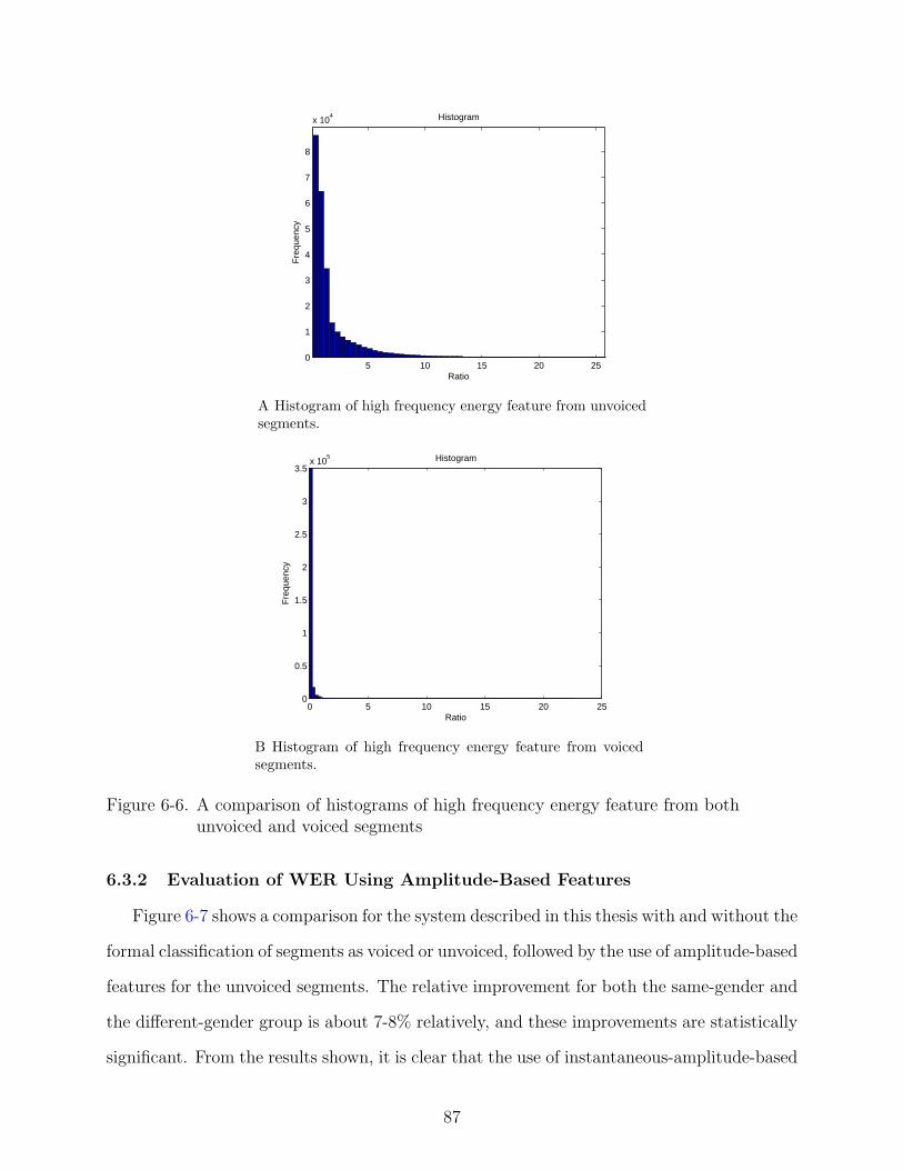
5 10 15 20 250
1
2
3
4
5
6
7
8
x 104
Ratio
Fre
quen
cy
Histogram
A Histogram of high frequency energy feature from unvoicedsegments.
0 5 10 15 20 250
0.5
1
1.5
2
2.5
3
3.5x 10
5
Ratio
Fre
quen
cy
Histogram
B Histogram of high frequency energy feature from voicedsegments.
Figure 6-6. A comparison of histograms of high frequency energy feature from bothunvoiced and voiced segments
6.3.2 Evaluation of WER Using Amplitude-Based Features
Figure 6-7 shows a comparison for the system described in this thesis with and without the
formal classification of segments as voiced or unvoiced, followed by the use of amplitude-based
features for the unvoiced segments. The relative improvement for both the same-gender and
the different-gender group is about 7-8% relatively, and these improvements are statistically
significant. From the results shown, it is clear that the use of instantaneous-amplitude-based
87
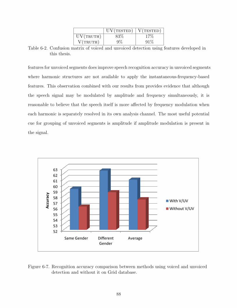
UV(tested) V(tested)UV(truth) 83% 17%V(truth) 9% 91%
Table 6-2. Confusion matrix of voiced and unvoiced detection using features developed inthis thesis.
features for unvoiced segments does improve speech recognition accuracy in unvoiced segments
where harmonic structures are not available to apply the instantaneous-frequency-based
features. This observation combined with our results from provides evidence that although
the speech signal may be modulated by amplitude and frequency simultaneously, it is
reasonable to believe that the speech itself is more affected by frequency modulation when
each harmonic is separately resolved in its own analysis channel. The most useful potential
cue for grouping of unvoiced segments is amplitude if amplitude modulation is present in
the signal.
����������������������
�� �������� ����������������
�������
��������
������������� !������
Figure 6-7. Recognition accuracy comparison between methods using voiced and unvoiceddetection and without it on Grid database.
88

CHAPTER 7SUMMARY AND CONCLUSIONS
In this dissertation, we have discussed an algorithm for instantaneous-frequency-based
cross-channel correlation to deal with the very challenging task of speech separation when
only one microphone is available.
Various instantaneous frequency estimation methods are covered in situations where the
clean speech signal is not available and is mixed with an interfering speaker. Following
the discussion about the estimation of instantaneous frequency, a discussion of how to use
cross-channel correlation to select frequency channels from the same harmonic structure is
presented, where simple averaging and the graph-cut method are discussed. In order to
improve the separation results, the use of amplitude-based features is considered for the
unvoiced segments, based on a detection of the voiced-unvoiced boundaries. Finally, the use
of a sieve function and other techniques are also introduced to maximize the final performance
of the separation system.
7.1 Major Findings and Contributions
The primary contribution of this dissertation is the development of a speech separation
algorithm that uses instantaneous-frequency-based temporal features to reconstruct a desired
speech signal that is presented in the presence of an interfering signal. THe system is based
on the CASA architecture. A detailed list of all contributions are given below.
• Introduction of a new approach to separate simultaneous speech using instantaneousfrequency.
• Use of pair-wise correlation based on estimated instantaneous frequency to find harmonicstructures and efficiently segregate frequency components.
• se of the mean square difference, harmonic sieve and other methods as complementarytools to improve the noisy information contained in the correlation patterns.
• Utilization of graph cuts as an optimal solution to extract information from the pair-wisecorrelation results.
• Attainment of better performance in terms of WER by implementing a bottom-upinstantaneous-frequency-based system.
89
7.2 Directions of Possible Future Research
Even with the performance improvements presented in this dissertation, single channel
speech separation solutions are still far from perfect. Using instantaneous-frequency-based
methods, there are several issues that could be improved in future research.
7.2.1 Combine long term and short term cross-channel correlation
Accurately estimating instantaneous frequency in noisy environments is remains challenging,
and certainly more work in this area is possible. One possible approach would be to
combine correlation estimates spanning very long durations with the present short-duration
correlations. Long-duration correlations (e.g. across the entire utterance) could be used
to identify several frequency channels which are highly correlated with each other globally.
This information can give the system a rough idea how to limit the detailed local search
to certain frequency regions, where short duration correlation would be applied to further
refine the final correlation results.
7.2.2 Combine instantaneous frequency and amplitude
While instantaneous frequency is shown in this study to be useful for speech separation,
other work in the literature has demonstrated the possibility of using instantaneous amplitude
as another important cue. One possible solution is first to estimate the instantaneous
amplitude and frequency as two independent features for each time-frequency cell and later
combine these two features in the feature space to construct a two-dimensional distribution
given certain amount of training data. With the known SNRs for the training data, a
proper model have two distributions for reliable and unreliable time-frequency cells can be
constructed. Finally, in evaluating simultaneous speech, the a posteriori probabilities can
be computed to determine the extent to which a processed cell is reliable.
7.2.3 Introduce image processing algorithms for mask generation
Generating an accurate binary mask for unvoiced segments can greatly boost the final
performance. In contrast to voiced segments, unvoiced segments lack of a clean and regular
harmonic structure. In order to segregate time-frequency cells into proper regions, image
90
processing algorithms can be imported here, especially for some image erosion, fill, and edge
detection algorithms. By using the eroding algorithms, many noisy time-frequency cells can
be ignored and integrated into the final process without too much distraction. Fill and
edge detection algorithms can also efficiently define where each time-frequency cell will be
assigned for the purpose of regrouping procedure.
7.3 Summary and Conclusions
In this dissertation, a new single-channel speech-separation approach based on instantaneous
frequency detection and cross-channel correlation is presented and evaluated. Using two
different databases, we demonstrated that separation using instantaneous frequency provides
better recognition accuracy than separation based on fundamental frequency alone, separation
based on instantaneous amplitude information, and baseline processing using MFCC features.
91

REFERENCES
[1] T. Abe, T. Kobayashi, and S. Imai, Robust pitch estimation with harmonics enhance-ment in noisy environments based on instantaneous frequency, Proceedings of ICSLP1996, 1996, pp. 1292–1300.
[2] L. Atlas and C. Janssen, Coherent modulation spectral filtering for single-channel musicsource separation, Proceedings of ICASSP 2005, 2005, pp. IV461–IV464.
[3] F. Bach and M. Jordan, Discriminative training of hidden markov models for multiplepitch tracking, Proceedings of ICASSP 2005, 2005, pp. V489–V492.
[4] S.P. Bacon and D.W. Grantham, Modulation masking: Effects of modulation frequency,depth and phase, Journal of Acoustic Society of America 85 (1989), 2575–2580.
[5] J. Barker, A. Coy, N. Ma, and M. Cooke, Recent advances in speech fragment decodingtechniques, Proceedings of Interspeech 2006, 2006, pp. 85–88.
[6] C. Bey and S. McAdams, Schema-based processing in auditory scene analysis, vol. 64,2002.
[7] B. Boashash, Estimating and interpreting the instantaneous frequency of a signal – part1: fundamentals, Proceedings of the IEEE 80 (1992), 520–538.
[8] , Estimating and interpreting the instantaneous frequency of a signal – part 2:algorithms and applications, Proceedings of the IEEE 80 (1992), 540–568.
[9] A.S. Bregman, Auditory scene analysis, MIT Press, Cambridge, MA, 1990.
[10] F.J. Charpentier, Pitch detection using the short-term phase spectrum, Proceedings ofICASSP 1986, 1986, pp. 113–116.
[11] M. Cooke, Grid corpus, Website, http://www.dcs.shef.ac.uk/spandh/gridcorpus/.
[12] , Interspeech 2006 speech separation challenge, Website, 2006, http://www.dcs.shef.ac.uk/~martin/SpeechSeparationChallenge.htm.
[13] M. Cooke, Jon Barker, Stuart Cunningham, and Xu Shao, An audio-visual corpusfor speech perception and automatic speech recognition, The Journal of the AcousticalSociety of America 120 (2006), 2421–2424.
[14] A. de Cheveigne and H. Kawahara, Multiple period estimation and pitch perceptionmodel, speech communication 27 (1999), 175–185.
[15] , Yin, a fundamental frequency estimator for speech and music, Journal ofAcoustic Society of America 111 (2002), 1917–1930.
[16] M. Dolson, The phase vocoder: A tutorial, Computer Music Journal 10 (1986), 14–27.
92

[17] Richard Duda, Peter Hart, and David Stork, Pattern classification, Wiley, John andSons, New York, 2000.
[18] G. Edelman, W. Gall, and W. Cowan, Auditory function: Neurobiological bases ofhearing, Wiley and Sons Press, New York, 1988.
[19] J. L. Flanagan and R. M. Golden, Phase vocoder, Bell System Technical Journal (1966),1493–1509.
[20] D.J. Hermes, Measurement of pitch by subharmonic summation, The Journal of theAcoustical Society of America 83 (1988), 257–264.
[21] G. Hu and D.L. Wang, Monaural speech segregation based on pitch tracking and ampli-tude modulation, IEEE Transactions on Neural Networks 15 (2004), 1135–1150.
[22] J. F. Kaiser, On a simple algorithm to calculate the energy of a signal, Proceedings ofICASSP 1990, 1990, pp. 381–384.
[23] , On teager’s energy algorithm and its generalization to continuous signals,Proceedings of 4th IEEE Digital Signal Processing Workshop, 1990, pp. 127–130.
[24] E. Kandel, J. Schwartz, and T. Jessell, Principles of neural science, Elsevier, New York,1991.
[25] B.E.D. Kingsbury, N. Morgan, and S. Greenberg, Robust speech recognition using themodulation spectrogram, speech communication 25 (1998), 117–132.
[26] A. Kusumoto, T. Arai, T. Kitamura, M. Takahashi, and Y. Murahara, Modulationenhancement of speech as a preprocessing for reverberant chambers with the hearing-impaired, Proceedings of ICASSP 2000, 2000, pp. 853–856.
[27] M. Lagrange and S. Marchand, Estimating the instantaneous frquency of sinusoidalcomponents using phase-based methods, Journal of the Audio Engineering Society 55(2007), 385–399.
[28] Q. Li and L.E. Atlas, Coherent modulation filtering for speech, Proceedings of ICASSP2008, 2008, pp. 4481–4484.
[29] P. Margos, J. F. Kaiser, and T. F. Quatieri, Energy separation in signal modulations withapplications to speech analysis, IEEE Trans. Signal Processing 41 (1993), 3024–3051.
[30] M.Weintraub, A computational model for separating two simultaneous talkers,Proceedings of ICASSP 1986, 1986, pp. 81–84.
[31] Jon Nedel, Duration normolization for robust recognition of spontaneous speech via miss-ing feature methods, Ph.D. thesis, Carnegie Mellon University, 2004.
[32] S. Palmer, Vision science, MIT Press, Cambridge, MA, 1999.
[33] J. Pickles, An introduction to the physiology of hearing, Academic Press, London, 1988.
93

[34] M. R. Portnoff, Implementation of the digital phase vocoder using the fast fourier trans-form, IEEE Trans. Acoustic., Speech, Signal. Processing 24 (1976), 243–248.
[35] P. J. Price, W. M. Fishe, J. Bernstein, and D. S. Pallett, The darpa 1000-word resourcemanagement database for continuous speech recognition, Proceedings of ICASSP 1988,1988, pp. 651–654.
[36] L. Rabiner, A tutorial on hidden markov models and selected application in speech recog-nition, Proceedings of the IEEE 77 (1989), 257–286.
[37] L. R. Rabiner and R. W. Schafer, Digital processing of speech signals, Prentice-Hall,Englewood Cliffs, NJ, 1978.
[38] D.A. Reynolds and R.C. Rose, Robust text-independent speaker identificiation usinggaussian mixture speaker models, IEEE Transactions on Speech and Audio Processing3 (1995), 72–83.
[39] S.M. Schimmel and L.E. Atlas, Coherent envelope detection for modulation filtering ofspeech, Proceedings of ICASSP 2005, 2005, pp. I221–I224.
[40] S.M. Schimmel, L.E. Atlas, and K. Nie, Feasibility of single channel speaker sepa-ration based on modulation frequency analysis, Proceedings of ICASSP 2007, 2007,pp. IV605–IV608.
[41] Steven M. Schimmel, Theory of modulation frequency analysis and modulation filtering,with application to hearing devices, Ph.D. thesis, University of Washington, 2007.
[42] F. Sha and L.K. Saul, Real-time pitch determination of one or more voices by nonneg-ative matrix factorization, Proceedings of Advances in Neural Information ProcessingSystem 17, 2005, pp. 1233–1240.
[43] J. Shi and J. Malik, Normalized cuts and image segmentation, IEEE Transactions onPattern Analysis and Machine Intelligence 22 (2000), 888–905.
[44] R. Sluyter, H. Kotmans, and T. Claasen, Improvements of the harmonic-sieve pitchextraction scheme and an appropriate method for voiced-unvoiced detection, Proceedingsof ICASSP 1982, 1982, pp. VII188–VII191.
[45] R. Sluyter, H. Kotmans, and A. Leeuwaarden, A novel method for pitch extraction fromspeech and a hardware model applicable to vocoder systems, Proceedings of ICASSP1980, 1980, pp. V45–V48.
[46] A. Takayuki, T. Mahoro, K. Noboru, T. Yukiko, and M. Yuji, On the important modula-tion frequency bands of speech for human speaker recognition, Proceedings of Interspeech2000, 2000, pp. III774–III777.
[47] N. Viemeister, Temporal modulation transfer functions for audition, The Journal of theAcoustical Society of America 53 (1973), 312–312.
94
[48] , Modulation thresholds and temporal modulation transfer functions, The Journalof the Acoustical Society of America 60 (1976), S117–S117.
[49] , Temporal modulation transfer functions based upon modulation thresholds, TheJournal of the Acoustical Society of America 66 (1979), 1364–1380.
[50] D. Wang and G. Brown, Computational auditory scene analysis: Principles, algorithmsand applications, Wiley-IEEE Press, New York, 2006.
[51] M. Wu, D.L. Wang, and G.J. Brown, A multipitch tracking algorithm for noisy speech,IEEE Transactions on Speech and Audio Processing 11 (2003), 229–241.
[52] W. Yost and S. Sheft, Across-critical-band processing of amplitude-modulated tones, TheJournal of the Acoustical Society of America 85 (1989), 848–857.
[53] , A comparison among three measures of cross-spectral processing of amplitudemodulation with tonal signal, The Journal of the Acoustical Society of America 87(1990), 897–900.
[54] W. Yost, S. Sheft, and J. Opie, Modulation interference in detection and discriminationof amplitude modulation, The Journal of the Acoustical Society of America 86 (1989),2138–2147.
95
BIOGRAPHICAL SKETCH
Lingyun Gu was born in Nanjing, Jiangsu, P.R. China. He received his B.S. in Electrical
Engineering from University of Electronic Science and Technology of China, Chengdu, Sichuan,
P.R. China in 1998 and M.S. in Electrical and Computer Engineering from Old Dominion
University, Norfolk, VA in 2002, respectively. Now he is a PhD student in Language
Technologies Institute, School of Computer Science at Carnegie Mellon University, Pittsburgh,
PA.
96