BLIND SOURCE SEPARATION OF SPEECH SIGNALS

USING FILTER BANKS

by

ANDREW J. PATTERSON, B.S.E.E., B,S,

A THESIS

IN

ELECTRICAL ENGINEERING

Submitted to the Graduate Faculty

of Texas Tech University in Partial Fulfillment of the Requirements for

the Degree of

MASTER OF SCIENCE

IN

ELECTRICAL ENGINEERING

Approved

August, 2002

ACKNOWLEDGMENTS

I would like to thank my advisor, Dr. Tanja Karp, for her patience and guidance

throughout this research. Her willingness to answer my "five minute questions" saved

me many hours of tedious labor. In addition, I would like to thank Dr. Sunandra

Mitra for providing the financial support that allowed me to concentrate on my thesis

and research and not where my next meal would be coming from. I am also thankful

for the guys, Cary, Cody, Jono, Mike, and Ryan for helping me remember that there is

more to life than work and school, most notably, cards, softball, and Josie's burritos!

I am very thankful for my wonderful parents whose unwavering love and support

is appreciated more than they could ever know. Thank you for teaching me diligence

and the value of a job well done.

Most of all I thank my loving wife for her support and understanding during

my late hours completing this thesis. Her love and encouragement kept me sane

throughout this paper.

11

CONTENTS

ACKNOWLEDGMENTS ii

ABSTRACT v

LIST OF TABLES vi

LIST OF FIGURES vii

I. GENERAL INTRODUCTION 1

1.1 Psychoacoustics 3

II. FILTER BANKS 6

2.1 Introduction 6

2.2 Delay 8

2.3 Examples 10

2.4 Gain Effects on Signal Reconstruction 12

III. BLIND SOURCE SEPARATION 14

3.1 Introduction 14

3.2 Literature Review 15

3.3 Higher-Order Statistics Overview 15

3.4 Higher-Order Statistics Approaches 16

3.4.1 Second-Order Information 16

3.4.2 Higher-Order Approximations 17

3.5 Whitening 18

3.6 JADE 21

3.7 Example 21

IV. IMPLEMENTATION 23

4.1 Introduction and Results 23

4.2 Testing Setup 24

4.3 Results 24

4.3.1 Results With No Psychoacoustic Model 24

4.3.2 Subband Power Correction 30

m

V. SUMMARY AND CONCLUSION 35

5.1 Future Work 35

BIBLIOGRAPHY 37

IV

ABSTRACT

The aim of this thesis is to improve the perceived quality of digital hearing aids

1 hrough the introduction of source segregation algorithms that attenuate undesired

speech and noise into the psychoacoustic model of the human ear. It proposes the

use of low-delay modulated filter banks to mimic the critical bands of the human ear

to accomplish blind source separation. This thesis will cover theory and results for

modulated filter banks and blind source separation.

LIST OF TABLES

4.1 Magnitude Square Error of Separated Signals for Figures 4.2 and 4.5 26

4.2 Magnitude Square Error of Separated Signals for Figures 4.4 and 4.5 28

VI

LIST OF FIGURES

1.1 Threshold in Quiet 4

1.2 Critical Bandwidth versus Frequency 5

2.1 Block Diagram of a /C-Decimated Filter Bank 6

2.2 Prototype Design with Linear Phase 9

2.3 Prototype Design with Raised (Dosine 10

2.4 Raised-Cosine: M=4, N=16, D=7 11

2.5 Raised-Cosine: M=4, N=24, D=7 11

2.6 Raised-Cosine: M=4, N=24, D=15 11

2.7 Linear Phase: M=4, N=24, D=15 11

2.8 Analysis Filters from Prototype in Figure 2.4 12

2.9 Synthesis Filters from Prototype in Figure 2.4 12

3.1 Joint Distribution of Unmixed Signals sx, S2 19

3.2 Joint Distribution of Observed Mixed Signals xi, a;2 20

3.3 Joint Distribution after Whitening the Mixtures 20

3.4 Example of BSS using JADE 22

4.1 Flow Diagram of the BSS Filter Bank Method 23

4.2 Separated Signal 1 using a 4-Channel Filter Bank with K = I . . . . 25

4.3 Separated Signal 2 using a 4-Channel Filter Bank with K = 1 . . . . 26

4.4 Separated Signal 1 using a 4-Channel Filter Bank with K — 2 . . . . 27

4.5 Separated Signal 2 using a 4-Channel Filter Bank with K = 2 . . . . 27

4.6 Separated Signal 1 using a 64-Channel Filter Bank with K = 32 . . . 29

4.7 Separated Signal 2 using a 64-Channel Filter Bank with i^ = 32 . . . 29

4.8 Separated Signal 1 using a 64-Channel Filter Bank with K = 32 and subband Power Correction 31

vu

4.9 Separated Signal 2 using a 64-Channel Filter Bank with K = 32 and subband Power Correction 31

•1.10 Analysis Filters for a Psychoacoustic Model of the Critical Band . . . 32

1.11 Synthesis Filters for a Psychoacoustic Model of the Critical Band . . 33

4.12 Separated Signal 1 using a Critical Band Approximation Filter Bank with K = 4 and subband Power Correction 34

4.13 Separated Signal 2 using a Critical Band Approximation Filter Bank with K = A and subband Power Correction 34

Vlll

CHAPTER I

GENERAL INTRODUCTION

Hearing impairment affects approximately 28 million people in the United States

and approximately ten percent of the total world population [1]. Hearing loss severity

can range from mild to so severe that communication is impossible without the use of

a hearing instrument. Despite the severity of the impairment, most hearing impaired

persons have trouble understanding a single speaker in the presence of background

noise or a mixture of speech segments- the so-called cocktail party effect. This is due

to damage in the cochlea of the ear, which results in a broader frequency selectivity

and a reduced dynamic range of the ear. This damage causes a rapid increase in

the sensation of loudness and a lass effective rejection of background noLse. The aim

of this thesis is to improve the perceived quaUty of digital hearing aids through the

introduction of source segregation algorithms that attenuate undesired speech and

noise into the psychoacoustic model of the human ear.

Since concurrent speech segments from different speakers have similar spectral

properties, it is impossible to remove the undesired parts from the desired one through

spectral filtering. Thus more elaborate methods need to be used. Blind source sep­

aration [5] is emerging as a technique that allows one to nearly perfectly segregate

different sources without any need of a priori knowledge on the statistical distribu­

tions of the sources or the nature of the process by which the source signals were

combined. Instead, it is generally assumed that the sources are statistically indepen­

dent and that the mixing model is finear. Based on these assumptions, the separation

algorithm attempts to invert the mixing process.

The drawbacks of current source separation algorithms are the slow speed of con­

vergence, the high computational complexity, and the number of microphones needed

(at least as many microphones as speakers). In the case of modem digital hearing aids,

(e.g., Phonak Claro), two microphones are available to perform beam-forming. Using

the above approach, it is thus possible to segregate two sources. This is sufficient to

1

our application if all undesired/background speakers can be combined to one noise

source. However, instead of applying source separation directly to the broadband

signals captured from the microphones, this thesis proposes to incorporate the source

separation with a filter bank that mimics the psychoacoustic model of the human ear.

Experiments have revealed that the peripheral auditory system behaves as a bank of

filters with increasing bandwidth towards high frequencies [18]. Its time-frequency

behavior has been successfully modelled through a wavelet filter bank [6, 16]. The

advantages of source separation in the subband domain compared to algorithms based

on broadband speech signals are as given:

• The frequency decomposition allows for treating frequency bands with different

hearing loss and different time-frequency sensitivity of the ear differently.

• Using a filter bank, the original computationally complex problem of separating

broadband speech signals can be split into a set of smaller parallel problems with

faster speed of convergence.

• Inherent speech statistical properties, such as different fimdamental frequen­

cies of different speakers, can be easily described in the frequency domain and

applied to the subband approach.

• An amplification of each subband depending on the hearing loss, which is de­

rived from an audiogram, can easily be introduced. This is aheady done in

commercial digital hearing aids.

This chapter presents a brief overview of psychoacoustic principles needed to fulfill

the project. The most important idea will be the concept of the critical band. Chapter

II will cover theory and implementation of low delay filter banks that will be used to

mimic the critical bands of the ear. Chapter III will introduce algorithms used for

blind source separation. Chapter IV will explain the method and implementation of

blind source separation using filter banks. Chapter IV will also present the results of

filter banks used in blind source separation and the psychoacoustic model. Finally,

Chapter V will give a conclusion of the work along with future work to be done in

this area.

1.1 Psychoacoustics

Psychoacoustics is the study of the psychological responses to acoustical stimuli.

In other words, psychoacoustics is the study of how the human brain perceives sound.

It takes into account what makes a sound loud, what determines pitch, etc. Human

hearing ranges from about 20Hz to 20kH2 [18]. Although hearing ranges up to 20kHz,

most of the energy of speech lies in the lower frequency band. In fact, intelligible

speech can be transmitted with a bandwidth of less than 5kHz.

Audibility of sounds is an important feature when performing speech processing

for hearing loss. The sound pressure needed for a tone to be just audible is not con­

stant across all firequencies. This threshold, called the threshold in quiet or absolute

threshold, is a function of frequency and is shown in Figure 1.1. This figure shows

how hearing loss caimot be overcome by simply amplifying the signal. Since each

frequency has a different absolute threshold, ampHfying the entire signal may make

some frequencies audible, but could also make other frequencies too loud and become

annoying or even painful to the patient. Hearing loss also affects different people

for different frequencies. Furthermore masking begins to occur. Masking refers to

the amount, or process, by which the absolute threshold is raised by the presence

of another sound (masker). Masking is what gives rise to the cocktail party effect.

Background noise and speech effectively mask out the desired speaker. Masking also

liO dB 120

I I I

^ " threshold of pain 10) dB 120

-100

80 gl .S

60 ^ (n g

iO c

20

Q02 a05 0,1 02 OS 1 2kHz 5 10 20 frequency

Figure 1.1: Threshold in Quiet. This figure is taken from [18, p. 15].

brings up another important topic in psychoacoustics: the critical bandwidth(critical

band). The critical bandwidth concept, introduced by Fletcher in 1940, states that

only a narrow band of frequencies surrounding a desired tone contribute to the mask­

ing of that tone [13]. In order for the tone to be masked, the power of the masker

inside the critical band must equal the power of the tone. All frequencies outside the

critical band do not contribute to masking. Figure 1.2 shows the critical bandwidth

versus frequency. In general, the critical bandwidth is about WOHz for / < 500Hz

and is about . 2 / for / > 500Hz. This works well since most of the information in

speech is located at lower frequencies. The ear provides better resolution at these

lower frequencies since the critical bandwidth is smaller for lower frequencies.

The critical band concept can be summed up with the following. An incoming

tone of frequency fc is mcident upon the ear. The ear then acts as a bandpass filter

with center frequency fc and bandwidth equal to the critical bandwidth at fc. Using

this concept it is possible to design a filter bank that imitates the critical bandwidths

of the ear.

5K lOK eoK

The critical bandwidth as a function of frequency at the center of the band.

20 90 100 200 500 IK ZK FREQUENCY (Hi>

Figure 1.2: Critical Bandwidth vs. Frequency. This figure is taken from [7, p. 235].

xtnl

H.(z) - i K

H,(2) * iK

H,(z) * i K

^ H,,W * iK

I

CHAPTER II

FILTER BANKS

2.1 Introduction

TK- F„(2)

! K - F,(2)

TK^ F,(2) ^

IHoti")!

I K - F„.,(2) J M-Channei liller bsnk decimeled by K

IH,(el«)l IH^,(>*OI

q d\ -I JS M M

typical idea] responses

Figure 2.1: Block Diagram of a /VT-Decimated Filter Bank

The first step in the method proposed in this thesis will be incorporating filter

banks in the blind source separation scheme in order to possibly achieve better pro­

cessing time. This section introduces filter bank theory necessary to understand the

overall method.

Filter banks are used in many applications such as subband coding for speech and

audio as well as for image coding. A filter bank simply divides a signal into subbands,

processes each subband, and reconstructs the signal. The analysis bank, Hk{z), sep­

arates the signal, and the synthesis bank, Fk{z) recombines it. The most simple filter

bank divides the signal into low frequency and high frequency channels(M = 2). This

of course can be expanded into any integer number. These are called M-channel filter

banks. A typical M-channel /C-decimated filter bank is shown in Figure 2.1. One

of the most popular filter bank is the cosine-modulated filter bank. For low-delay,

cosine-modulated filter banks, the analysis and synthesis filters are cosine-modulated

versions of a single prototype filter, i.e..

hk[n] = 2 . p[n] . cos [ ^ . (fc + 1) . (n - | ) -f {-1)'^] (2.1)

/4n] = 2 • p[n] • cos [ ^ • (fc + 1 ) . (n - | ) - (-!)*= J (2.2)

where M is the number of channels, N is the length of the prototype filter p[n],

and D is the desired overall delay [8]. Another popular filter bank is the complex-

modulated filter bank. This is similar to the cosine-modulated filter bank, except

the analysis and synthesis filters are calculated by modulating the prototype by a

complex exponential, i.e.,

hk[n] - V2 • p[n] • e^'^^"-^) (2.3)

fk[n] = V2 • q[n] • e^''^("-f) (2.4)

In many cases, p[n] = q[n\. Prototypes designed for an M channel cosine-modulated

filter bank are the same for a 2M channel complex-modulated filter bank [17]. The

objective is to design the prototype filter to meet the desired specifications. In many

audio applications, it is desired to have the stopband attenuation on the order of

30 dB. For perfect-reconstruction filter banks, these specifications can be hard to

satisfy. It may be sufficient to allow a small reconstruction error. By allowing some

reconstruction error, a higher stopband attenuation may possibly be achieved by

using near-perfect-reconstruction (NPR) filter banks. NPR filter banks allow a small

aliasing component in the reconstruction of the signal. In most appUcations, the

added aliasing is considered negligible because the ear is not able to discriminate this

error. However, tolerating this aliasing component may allow us to achieve a higher

stopband attenuation.

This thesis uses an algorithm proposed by Nguyen to design prototype filters

suitable for a low-delay modulated filter banks [14]. This algorithm designs prototype

filters that minimize the power in the stopband. In other words, it finds h[n] that

minimizes /»7r

/ \H{e''^)f duj Ws is the stopband frequency. (2.5)

Eq. 2.5 written in quadratic form gives,

h*Ph - min (2.6)

7

where

n.i = 2 X ] A / " cos a;(fc - /) du. (2.7)

Here, 5 is the number of stopbands of H{e^'^), Pi are there relative weights, and uJij

and cjj 2 are the bandedges of the stopbands. The minimization is subject to the

constraint that h[n] is a 2M*'' band filter. This means that shifted versions of H{z)

sum up to a constant value in the frequency domain. This ensures that no amplitude

distortion occurs after reconstniction of the input signal.

2.2 Delay

Another important feature of a filter bank is the overall system delay. For hearing

aid appfications, if the delay becomes longer than 10ms, many annoying side effects

occur, such as echoing. In the case of linear phase filters, the delay of a system

depends upon the length of the filters used. If we design a linear phase prototype,

the overall delay of the system is A'' — 1, since both the analysis and synthesis filters

both introduce a delay of {N — l) /2 . If we are not constrained to linear phase filters,

we can possibly achieve a higher stopband attenuation by increasing the length of

the filter, but not the delay. In other words, we can begin with a Unear phase filter

with a length equal to the delay and then pad the "tail" with zeros, as shown in

Figure 2.2. We then use the Nguyen algorithm mentioned above to optunize the

filter. We can also use a raised-cosine window as our beginning filter, as shown

in Figure 2.3. By padding the "tail" of our prototype filter, we can increase the

stopband attenuation without effectively increasing the delay. There is, however, a

limit to the advantage gained by this technique since the coefficients of the optimized

filter approach zero as the length approaches infinity. These smaller filter coefficients

will contribute negfigible stopband attenuation. Prototypes designed with a raised-

cosine starting point generally produce better optimized filters. This is because the

algorithm proposed by Nguyen does not produce a global solution. Hence better

starting points produce a better optimized filter.

-e—«——e—«—8—*—e—e 10 12 14 16

Figure 2.2: Prototype Design with Linear Phase

The basic steps of the algorithm proposed by [14] are as follows:

1. Compute the stopband power matrix P, where the (fc — /)*'' element is

[PI t^i = 2 Y j Pi I cos a;(fc — I) do;.

2. Unless a starting point is given, design an initial starting point, usually a raised-

cosine filter is used as the starting point.

3. Compute the quadratic conditions, h*Snh. Here, 5„ is a matrix ensuring that

h[n] is a spectral factor of a 2M*'' band filter.

4. Compute the stopband error, h'^Ph.

5. Solve the quadratic-constrained minimization problem,/i*Fi'i = min, subject to

h'Snh = 0.

6. Use the optimized prototype filter to calculate the analysis, /i^, and synthesis

filters,/fc.

<

1

1

(

p

<

1

1 ( J

1

r

1

( 1

< )

(

—o

- G

e— LA

.

1 1

1 1

1 1

Figure 2.3: Prototype Design with Raised Cosine

7. The overall filter bank response is then calculated by convolving hk with fk and

summing the result.

2.3 Examples

To illustrate this method of prototype filter design, examples will be presented in

this section. We will show how increasing the length of a filter without increasing

the delay can provide higher stopband attenuation. Figure 2.4 shows the initial and

optimized prototype filters for M = 4, N = 16, and D = 7 with a raised-cosine filter

as the starting point. We can see that the stopband attenuation of the optimized

filter is about 30dB. Figure 2.5 shows the initial and optimized filters for M = 4,

N = 24, and D — 7. For this filter, the stopband attenuation of the optimized filter

is about 32dB. We have increased the attenuation by 2dB without increasing the

system delay. Figure 2.6 shows the filter responses with M = 4, iV = 24, and D = 15.

It is obvious that increasmg the delay also hicreases the attenuation of the filter, but

as mentioned before, this may be unacceptable for speech processing applications.

Figure 2.7 shows the prototype response for M = 4, A = 24, and Z) = 15 with a

10

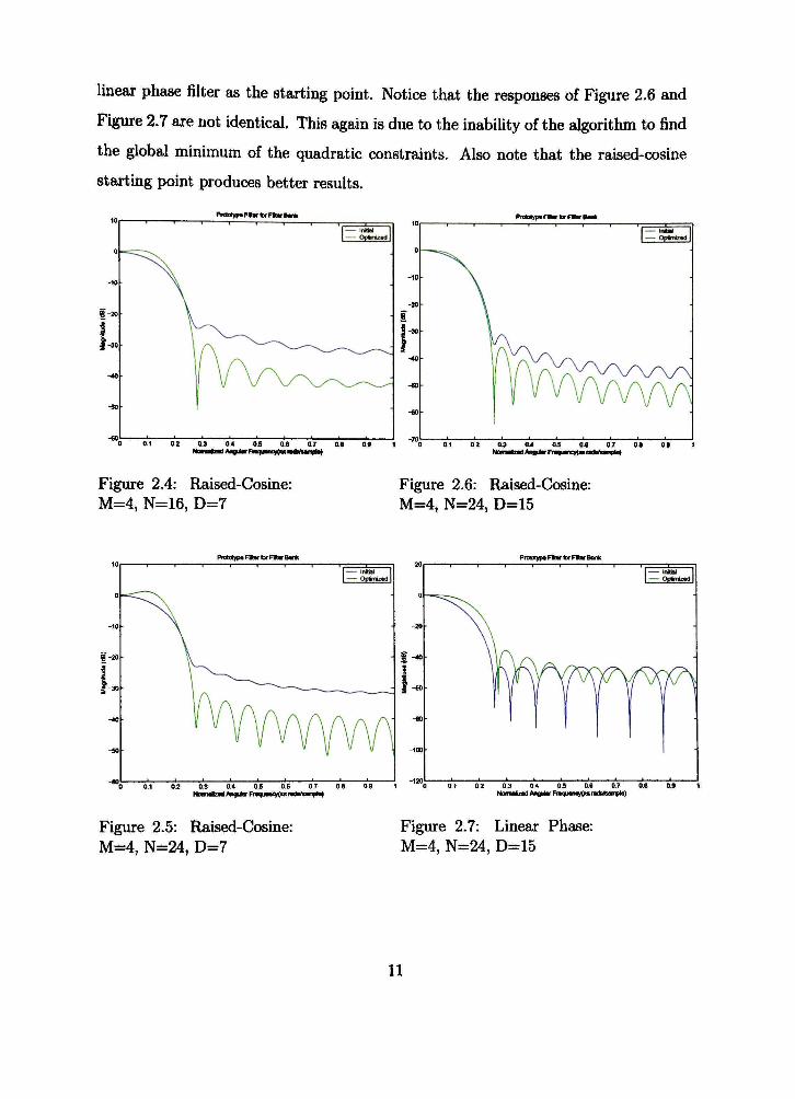
linear phase filter as the starting point. Notice that the responses of Figure 2.6 and

Figure 2.7 are not identical. This again is due to the inability of the algorithm to find

the global minimum of the quadratic constraints. Also note that the raised-cosine

starting point produces better results.

0

-10

§-20

1 jf-30

-40

-50

ProMyp* FHr ttr FIMr Bank

-

•

•

~\_----^-^

Prototype Filar fv Fllv eerti

0 0.1 0.2 0.3 _ 0.4 0.5 0.6 0.7 0.8 0.0 1 0 0.1 02 0.3 04 0.5 0.6 0.7 0.6 0.9 1 le) HoimMtalAiigdarFta«an(y(i«ra<hta>i«la)

Figure 2.4: Raised-Cosine: M=4, N=16, D=7

Figure 2.6: Raised-Cosine: M=4, N=24, D=15

10

0

-10

f-20

f

5-30

-40

-50

Prototype ntar far F H V Bank a I • 1 I . I

1 — Initial 1 1 — OpHmizrt 1

•

•

.

A A A"

' '

S

1 1

20

0

-20

-40

-60

-80

-100

PraUlypt FIMr far Fltir Bank

1 — inttH I 1 — Optntzedi

•

•

,

•

02 0.3 0.4 0.5 0.6 0.7 0.8 0.9 0.1 0.2 0.3 0.4 0.5 0.6 0.7 Nonnaizad Angular FnqMan fxx raiWMnTpta)

Figure 2.5: Raised-Cosine: M=4, N=24, D=7

Figure 2.7: Linear Phase: M=4, N=24, D=15

11

Figure 2.8 and Figure 2.9 show the analysis and synthesis filters of the prototype

design from Figure 2.4.

Figirre 2.8: Analysis Filters from Prototype in Figure 2.4.

i . L - I — . 1 -

0 0 1 0 2 0 3 0.4 0 5 0 6 0.7 0.8 OS 1 Normalized Angular Frsquencytm radsAarrpIs)

Figure 2.9: Synthesis Filters from Prototype in Figure 2.4.

2.4 Gain Effects on Signal Reconstruction

Processing a signal in the subband domain limits the ability of the filter bank

to reconstruct the signal. Once a gain is added to a subband it is impossible to

12

achieve perfect reconstruction, even if PR filter banks are used. Amplifying a subband

can contribute audible aliasing in the reconstnicted signal. This fact becomes a

problem when performing blind source separation in the subband domain. This will

be discussed in Chapter IV.

13

CHAPTER III

BLIND SOURCE SEPARATION

3.1 Introduction

Recovering sources from a mixture of several others is an important topic in signal

processing today. An example of when this is necessary is the so called cocktail party

problem. This problem occurs when two people are trying to communicate while in

a situation with loud background noise. In this example, the voice of one person is

mixed with many other sounds of the party. A good human ear can easily extract

the wanted voice, but it is much more difficult for machines or persons with a hearing

impairment. Independent component analysis and, more importantly, bfind source

separation are techniques to allow us to segregate different sources.

Bfind source separation (BSS) attempts to recover unobserved signals or "sources"

from several observed mixtures. For speech processing, these observations are the

measurements at the output of different microphones. Each microphone receives

a different combination of the sources. "Blind" in this context stresses that the

sources are not observed and information about the mixture (i.e., channel) is not

known. Instead we assume that the source entries are independent and some a priori

information about the distribution of the sources might be available.

The simplest BSS model assumes n source signals Si(t),52(t),... ,s„(t) and the

measured observations of m mixtures xi{t),X2{t), ...,Xm{f)- We must have at least

as many observations (microphones) as we do sources, i.e., m > n [5]. Throughout

this paper it is assumed that m = n. These mixtures are assumed to be linear and

instantaneous ^ In other words

Xi{t) = ^aij •Sj{t)

i = l

for each i = 1 . . . n. This process can be represented in matrix form by the equation,

x{t) = A - s{t) (3.1)

^Convolutive mixtures are also addressed [i.e., [11], [15]], but are not the scope of this paper

14

where s{t) = [si{t), .93(i),..,, .s„(<)] is an n x 1 column vector of the source signals

and x{t) = [xi{t),X2{t),...,Xn{t)] are the n observed signals, and A is the mixing

matrix of dimension n x n. The BSS problem is recovering the source vector s{t)

using only the observed signals x{t) and possibly some a priori information about

the distribution of the inputs. So we wish to find a matrix B that separates the input

s{t) such that the output

y{t) - B • x{t) (3.2)

is an estimate of the source signals s{t).

3.2 Literature Review

The foundations of BSS were laid out by Comon, Herault, and Jutten [10]. Comon

extended principal component analysis to help solve this problem. Independent com­

ponent analysis was developed following his work.

Herault and Jutten approached the BSS problem using neural networks. They

used a gradient descent algorithm to estimate the mixing matrix A, thus allowing

them to separate the sources.

The groimdwork laid by these works lead to the development of new algorithms,

many of which are based on higher-order statistics. An approach developed by Car­

doso [3], called JADE, wiU be the main the topic of this paper.

3.3 Higher-Order Statistics Overview

The information in this section comes directly from [12]. Higher-order statistics

are used when dealing with non-Gaussian random processes. Since many real world

signals are non-Gaussian, higher-order statistic approaches are needed and can be

used to measure a signal's distance from being Gaussian. An advantage that higher-

order statistics has over second-order statistics is that they are able to provide phase

information. Higher-order statistics are also bUnd to Gaussian random processes since

their cumulants past second-order are zero. Thus cumulant based signal processing

techniques boost signal-to-noise ratio when signals are corrupted by Gaussian noise.

15

For most blind source separation algorithms, second-order and fourth-order cu­

mulants are used. For zero mean processes, which are assumed for BSS, second-order

cumulants are identical to second-order moments,

Cum[a,b]^E[ab]. (3.3)

Fourth-order cumulants are given by

Cum[a, b, c, d] = E[abcd\ - E[ab]E[cd] - E[ac]E[bd] - E[ad]E[bc]. (3.4)

These equations will be used in a later section to develop contrast functions for

achieving blind source separation.

One question that may surface is "Why do we need fourth-order cumulants in­

stead of just third-order cumulants?" For S3Tnmetrically distributed random process

the third-order cumulants are zero; thus fourth-order cumulants are needed. Another

question that needs to be answered is why we only use fourth-order cumulants in­

stead of higher-order moments. This is because the fourth-order cumulant of two

statisticaUy independent processes equals the sum of the cumulants of the individual

process. This however is not true for higher-order moments. This should provide

enough information in order to proceed to the blind source separation theory.

3.4 Higher-Order Statistics Approaches

3.4.1 Second-Order Information

Many researchers have worked on solutions to BSS based on second-order and

higher-order statistics. First we will cover the second-order approach. We begin by

re-writing the observation, x{t) — A • s{t) = z{t). Assuming independent sources we

can then formulate the sources by their covariance matrix [10],

Rs{r) = E[s{t-\-r)-s*{t)] =

^E[s,{t + T)-sl{t)] ••• 0 ^

\ 0 ••• E[sy{t + T)-sl{t)]J

16

(3.5)

Now the covariance matrix of the observations is given by

R^{t) = A • R,{T) • A". (3.6)

Remember that the goal of BSS is finding a matrix approximately equal to A. To

accomplish this we whiten the observed signal z{t) with a matrix W such that

W • R,{0) W" = W-A-A" -W" = r (3.7)

where / is the identity matrix. We also note that since Wis & whitening matrix, then

U = WA is an unitary matrix. It is the goal then to find the matrices W and U that

give an approximation of the mixing matrix A by

A = W-^U. (3.8)

Once the matrices W and U axe found , we can estimate the sources by

s{t) = U^ -W- x{t) = B • x{t). (3.9)

An algorithm to find the matrix W and U based on second-order statistics was pre­

sented by Belouchrani, et al [2].

3.4.2 Higher-Order Approximations

Second-order approaches work well when we are dealing with stochastic Gaussian

processes, since a Gaussian process can be completely characterized by its second-

order statistics, i.e., mean and variance. However, when the signals are not Gaussian

we must extend our concept to higher-order statistics, i.e., aimulants. Without the

use of these higher-order statistics, it is impossible to separate non-Gaussian signals.

Cardoso developed an algorithm called JADE that used higher-order statistics instead

of the second-order covariance matrix of z{t) [3]. He used the sample fourth-order

cumulants of the whitened process z{t) = W • x{t).

Using the knowledge from Eqs. (3.3) and (3.4), the cumulants of the output vector

y in Eq. (3.2) are

Cij[y] = Cum[yi, yj] and Cijki[y] = Cum[yi, yj, yk, yi]. (3.10)

17

Knowing that the source vector has independent entries, its cross-cumulants vanish,

giving us the equations

CiM = ^i^ij and djki = kiSijki (3.11)

where 6 is the Kronecker delta function and a? is the variance. The kurtosis k is

given as

h = E[st]-3E[s^]^ (3.12)

Using these equations we can measure the mismatch between the input source distri­

bution and the unmixed output distribution [10]. Measures in the quadratic mismatch

between cumulants are given by:

Hy] = J2(^^M-CiAs]r (3.13) ij

My] = Yl ( ^ - 'ty] - Qjkiis])^. (3.i4) ijkl

(j)2 is a contrast fimction using only second-order statistics whereas, (p^ is a fourth-

order cumulant contrast function. Cardoso has shown in [5] that under the whiteness

constraint </»2 = 0. Thus (j)4 is a sufficient contrast function if all the sources are known

to be non-Gaussian (i.e., non-zero kurtosis). Using 04 as the objective function, we

can minimize the mismatch between the two vectors, thus separating the sources.

This leads us to the JADE algorithm which wiU be described later.

3.5 Whitening

As mentioned in the introduction, in order to achieve source separation we assume

that the sources are independent and are zero mean. However, after the signals

become mixed by the matrix A, independence may no longer hold [9]. This is shown

by a simple example, based on [9], as shown in Figure 3.1 and Figure 3.2. We can

see from Figure 3.1 that si and S2 are completely independent, since for any given

value of si we cannot determine the value for S2- Figure 3.2 on the other hand

shows that observed signals xi and x^ are no longer independent. This is easy to

18

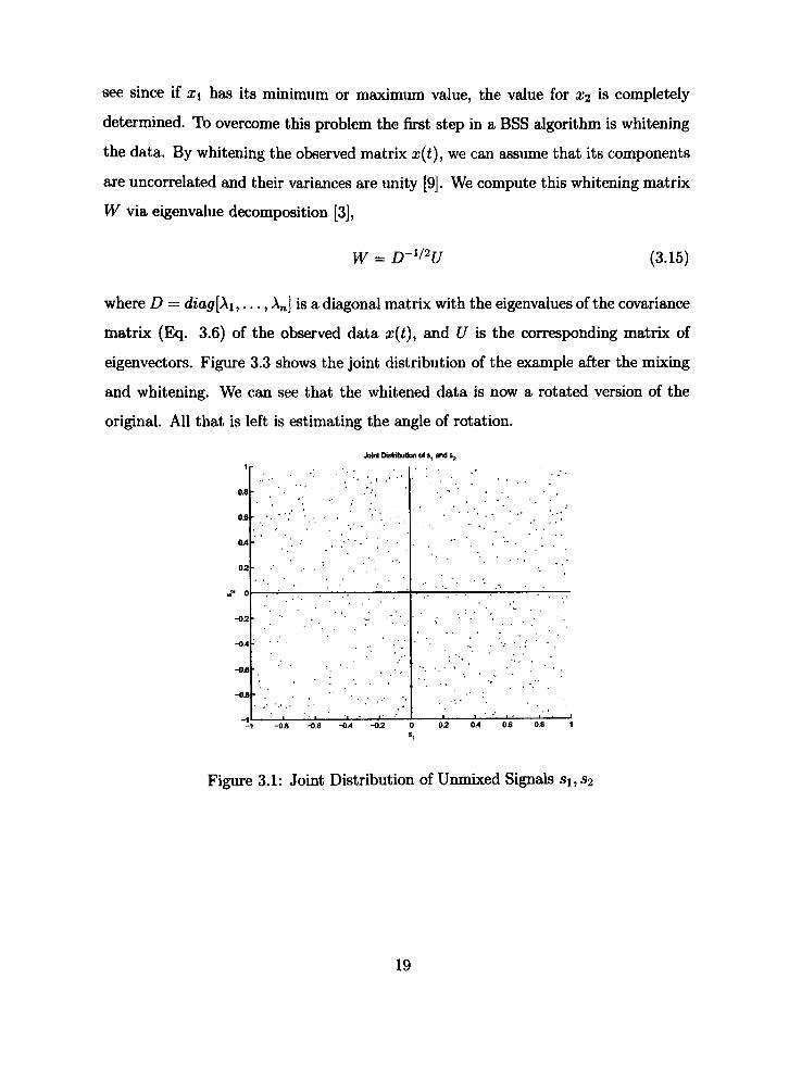
see since if xi has its minimum or maximum value, the value for X2 is completely

determined. To overcome this problem the first step in a BSS algorithm is whitenmg

the data. By whitening the observed matrix x{t), we can assume that its components

are uncorrelated and their variances are unity [9]. We compute this whitening matrix

W via eigenvalue decomposition [3],

W = D-^/^U (3.15)

where D = diag[Xi,..., An] is a diagonal matrix with the eigenvalues of the covariance

matrix (EJq. 3.6) of the observed data x{t), and U is the corresponding matrix of

eigenvectors. Figure 3.3 shows the joint distribution of the example after the mbcing

and whitening. We can see that the whitened data is now a rotated version of the

original. AH that is left is estimating the angle of rotation.

Joint DtsHbuHon of s, and s.

Figure 3.1: Joint Distribution of Unmixed Signals si, S2

19

A

3

2

J " 0

-1

-2

-3

Jdnt DbMullan o) ObMTVOd Mbibim x, and x^ Mxed

•

-

. • • . ' ; •

• ' • • • ^ - ' • ; , • '•:

- ' / • • . : : '

, . '•'" . * • ••. • • ' • . . • / ' ' •

. . " . • • • • • . ' • , ' • < • • •••••••

; • • ; ; ' •'••;'• : '•:• ' " : • • '

• ; • : . ' • • • '• . '• .• •

f- • •' ' . , '.

• ' " . • ••

• ^ .

' ,'

Figure 3.2: Joint Distribution of Observed Mixed Signals xi, X2

2.5

2

1.5

1

0.5

0

-0.5

- 1

-1.5

- 2

Jdnt Distribution after Whitening the Mixtures

• . . ' • ' ;

• ' . ' . • ' ' •

, . ' - * ' • ^ . . ' . .

» • . . . . • • ' " . • . " • . . ; . - " • . ; '

• • ' • ' . • ' • • . • ' . ' . . ^ '••._ : • : • • . • N ' ; ' • • • •

• ' • • • ; . ' . • • ' • • • ' • • • • ' ' . • : '

• • ' ' ' • '

* * . ". .

' -

1 1

-2.5 -2 -1.5 -1 -0.5 0.S 1 1.5 2 2.5

Figure 3.3: Joint Distribution after Whitening the Mixtures

20

3.6 JADE

Joint Approximate Diagonalization of Eigen-Matrices (JADE) is one algorithm to

achieve blind source separation [4] which uses higher-order statistics. The steps of

the JADE algorithm are as given:

1. Form the sample covariance matrix Rx of the observed signals and compute the

whitening matrix W as described in the previous section.

2. Estimate the fourth-order cumulants of the whitened process, z{t) = Wx{t).

Compute the n most significant pairs.

3. Jointly diagonalize the set by a unitary matrix U. For more details on joint

diagonaUzation, see [3].

4. The estimate of yl is ^ = W*U, where * denotes pseudo inverse((W^W^)~^l^^).

The separating matrix B is now given as B = U^W and the separated sources

are s{t) = Bx{t).

It is important to note that JADE returns the separated sources in order of highest

energy. This knowledge becomes important when incorporating BSS in the subband

domain. This will be discussed in Chapter IV.

3.7 Example

This is a simple example in which two sources, a sine wave and a square wave,

are mixed by a random mixing matrix. The JADE algorithm is used to separate

the signals. We use two sensors for this example. Figure 3.4 has the results of this

simulation. The first row shows the original sources. The second row shows the

two observed signals after they were instantaneously mixed. The final row shows

the separated sources. We can see by comparing rows 1 and 3 that the algorithm

successfuUy separated the mbced sources. We also note how the order has been

reversed implying that the square wave has higher energy.

21

200 200

\ N j r\

K & ^ J t-^ I I 200 200

200 200

Figure 3.4: Example of BSS using JADE

22

CHAPTER IV

IMPLEMENTATION

4.1 Introduction and Results

s, O- *y^ Analysis Filter Bank

SN O - •o^ Analysis Filter Bank

BSS yii

BSS

Synthesis Filter Bank

yioi

Synthesis Filter Bank

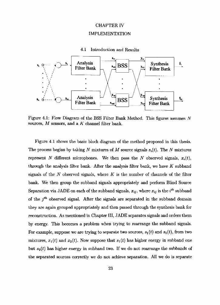
Figiu-e 4.1: Flow Diagram of the BSS Filter Bank Method. This figures assumes N sources, M sensors, and a K channel filter bank.

Figure 4.1 shows the basic block diagram of the method proposed in this thesis.

The process begins by taking N mixtures of M source signals Sj(f). The N mixtures

represent TV different microphones. We then pass the N observed signals, Xi{t),

through the analysis filter bank. After the analysis filter bank, we have K subband

signals of the N observed signals, where K is the number of channels of the filter

bank. We then group the subband signals appropriately and perform Blind Source

Separation via JADE on each of the subband signals, Xy, where Xij is the i*'* subband

of the J*'' observed signal. After the signals are separated in the subband domain

they are again grouped appropriately and then passed through the synthesis bank for

reconstniction. As mentioned in Chapter III, JADE separates signals and orders them

by energy. This becomes a problem when trying to rearrange the subband signals.

For example, suppose we are trying to separate two sources, Si{t) and S2{t), from two

mixtures, xi{t) and X2{t). Now suppose that si{t) has higher energy in subband one

but S2{t) has higher energy in subband two. If we do not rearrange the subbands of

the separated sources correctly we do not achieve separation. All we do is separate

23

the sources and then remix them in the subband domain. We must somehow be able

to estimate the source subband powers in order to be able to successfully achieve

separation.

4.2 Testing Setup

Matlab programs were written to implement the structure shown in Figure 4.1.

Speech signals in .wav format sampled at 1 IkHz were used for aU simulations. Results

for different setups will be given in this section. The problem of correctly rearrang­

ing the separated sources in the subband domain is overcome by usmg the original

source signals for comparison. Although this situation would not occur in practice,

since if we already knew the soiuces we would not bother estimating them from the

mixtures, it is good for baselining the method proposed by this thesis. For practical

implementations, estimates would have to be done, perhaps using the fundamental

frequency of the separated signals. Since separation for speech is not best quantified

by figures, a comment on the audible reconstruction quaUty will also be given. This

is a subjective measure of how weU the separated sources sounded when compared

to the originals. Separation is also carried out without the filter bank in order to

compare the filter bank's performance to the standard JADE algorithm.

4.3 Results

4.3.1 Results With No Psychoacoustic Model

This section presjents the results for the general case of Figure 4.1. This case uses

a uniform modulated filter bank. It has no psychoacoustic model.

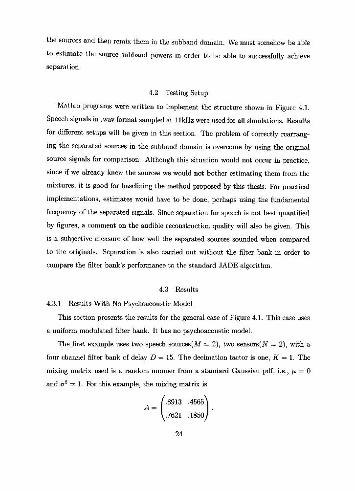
The first example uses two speech sources(M = 2), two sensors(A^ = 2), with a

four channel filter bank of delay D = 15. The decimation factor is one, K = \. The

mixing matrix used is a random number from a standard Gaussian pdf, i.e., // = 0

and cr = 1. For this example, the mixing matrix is

/.8913 .4565^ A ^ \

\^.7621 .1850 i

24

The results are shown in Figure 4.2. The first, second, and third rows are the original

signal, separated signal using the filter bank and the separated signal without the filter

bank, respectively. Disregarding any scaling, we can see from Figure 4.2 and Figure

4.3 that the separation seems to be good, especially for low frequencies. At higher

frequencies however, we see that the separation is trying to flatten the spectrmn out.

In other words the separation seems to be attempting to place the same power in all

subbands. We of course know that is not correct, especially for speech. This increase

in the higher subbands also contributes to what sounds like aliasing. Listening to

the separated signals and comparing them to the originals solidifies this statement.

Minor afiasing is heard in this example. When can also see from Table 4.1 that the

magnitude of the squared error also increases with frequency. In the table, wideband

is the error when no filter bank is used.

Original Signal «1(bigtip5_11.W3V)

« 20

2

I 0 z

-20

-lf%m 0 0.5

%[im^^^^ 1 1.5 2

Separated wllh K==1

i r v k ^ 25

Wp 3

•jf^k^^H^^

0 0.5

-^f%n 1 15 2

Separated wrthout the Filter Bank

V^*'**'\*ftW

2.5

( A * ^

3

^

Figure 4.2: Separated Signal 1 using a 4-Channel Filter Bank with K = 1

25

Original Signal *2(pathQkiglcaL11 wav)

(

60

I « 1 20

^ 0

-20

0.5 1 1.5 2 Separated wllhout the Hter Bank

f\ . / I , A k ^ J W V W v i A . / L *,L iil^u W " ^ « ^^¥%ffiim^f^ ' 1 1„.,.. 1 1

25

1 ' '

f*fW^

3

,

ffMf^

Figure 4.3: Separated Signal 2 using a 4-Channel Filter Bank with K = 1

Table 4.1: Magnitude Square Error of Separated Signals for Figures 4.2 and 4.5

subband # 1

subband # 2

subband # 3

subband # 4

Wideband

Signal 1

3.185641e-008

1.514488e-009

1.483576e-007

5.439991e-007

1.372496e-007

Signal 2

1.130017e-014

7.759092e-011

1.180485e-008

1.723980e-009

9.323691e-013

The next simulation was similar to the first except the decimation factor is two

{K = 2). The results are shown in Figures 4.4 and 4.5

26

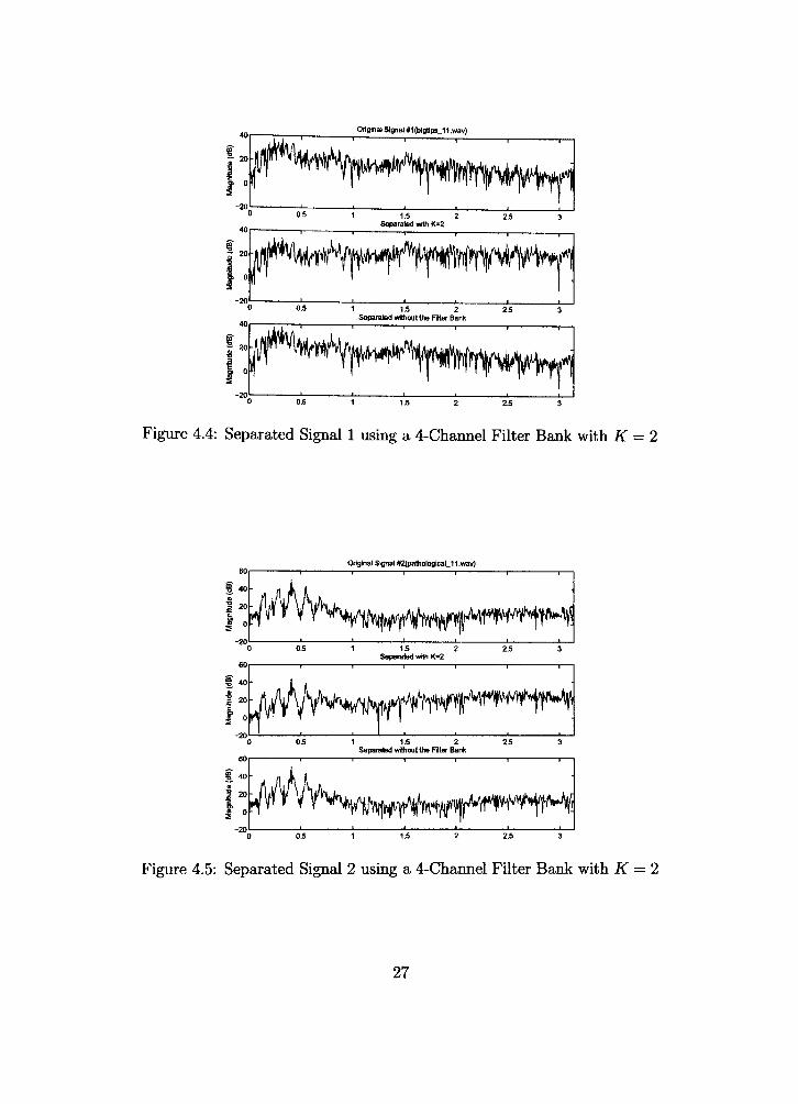
Original Slgnai#1(bigtips_11.wav)

Figure 4.4: Separated Signal 1 using a 4-Channel Filter Bank with K = 2

Original Signal #2(pathological_11.wav)

0 0.5

40

20

0 •ii/AV^ JVi» f '

1 15 2 Separated avnh K=2

imhM^iW^ wmfp w II

2.5

rfiW4v^*

3

W^

0 OS

20

0

„ i 1

•Mfh Pi V " T 1

1 15 2 Separated without the Filer Bank

"^ ^m0WW^0f*^

25

tMlM^ pifn^"

3

iWmhfi miw"m

Figure 4.5: Separated Signal 2 using a 4-Channel Filter Bank with K = 2

27

The decimation factor did not seem to play a significant role in the quaUty of

separation and the subband errors are comparable. The error is shown in Table 4.2.

We will assume for here forward that decimation does not affect the ability to separate

the signals as long as it is not critically decimated, i.e., decimated by the nmnber of

channels of the filter bank.

Table 4.2: Magnitude Square Error of Separated Signals for Figures 4.4 and 4.5

subband # 1

subband # 2

subband # 3

subband # 4

Wideband

Signal 1

2.615838e-008

3.172436e-009

2.842648e-007

2.283053e-006

1.372496e-007

Signal 2

2.49901 le-014

7.741295e-009

1.559634e-008

6.735304e-010

9.323691e-013

In order to determine the effects of small bandwidth filters, the next example uses

a filter bank with 64 chaimels with K = 32. Just as in the case for a four-channel filter

bank. Figures 4.6 and 4.7 show how each subband power tends to flatten out. This

causes poor results when the separated signals are compared to the originals. The

aliasing in this case is very noticeable and begins to become annoying. As mentioned

in Chapter II, the aliasing is most likely because of the gain that occurs during the

separation process. We know that adding a gain in a subband prohibits perfect

reconstruction and leads to afiasing. This gain must be overcome in order to achieve

a good estimation of the original sources. This is addressed in the next section.

28

Original Signal ^(b lg l lpa. l 1 .wav)

I »

-^fhm 0 0.5

^iprn^

0 0.5

r — 1 1 —

1 15 2 Separated with K°32

kMm^nm^

1 15 2 Separated without the Piter Bank

» ^

25

pif 25

^

3

wj 3

-f'^*'''*^^^ Figure 4.6: Separated Signal 1 using a 64-Channel Filter Bank with K = 32

Original Signal #2(pathotogical_11 .wav)

Figure 4.7: Separated Signal 2 using a 64-Channel Filter Bank with K = 32

29

4.3.2 Subband Power Correction

If Sn,k is a column vector denoting the fc"* subband of the n"* original signal and

T denotes the length of the vector, then the signal power in that subband is given as

Ps„,k = ^ \ /< fe -Vfc - (4.1)

Once we have the separated signal yfn,k we can calculate the power given by Eq. 4.1

as

Py'n,k = j;y/yflk-y'n,k. (4.2)

In order to try and compensate for the gain that may have been introduced in that

subband, we multiply the separated signal by the ratio of the powers given in Eqs.

4.1 and 4.2, Ps ,

yn,k = - ~ - • y'n,k- (4.3)

Hopefully this wiU minimize the effect of the introduced gain, and thus help minimize

the aliasing. Obviously this approach cannot be used in practical applications because

the original sources are not known. It does, however, provide information on whether

correcting the subband power is a topic to be further investigated.

Using the same filter bank that was used in the previous simulation we can verify

that correcting the power in each subband helps with the afiasing. For redundancy,

our filter bank has 64 channels and a decimation factor of 32.

These figures show how the subband power correction helps overcome the problem

of the algorithm attempting to make each subband power equal. The audibiUty

aliasing has also all but disappeared using the subband power correction approach.

The results in Figure 4.8 and Figure 4.9 confirm our hypothesis that the aliasing was

emerging from the subband power amplification. Thus it is necessary to somehow

correct the subband power to minimize the effects of afiasing.

30

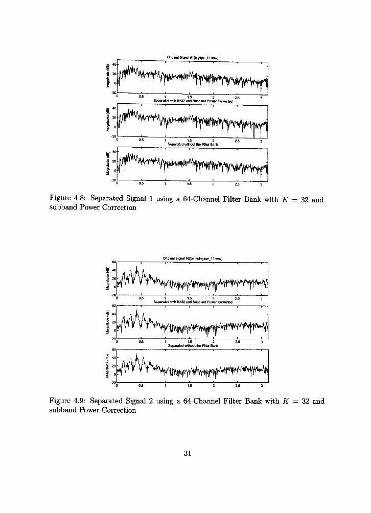
Original Signal «1(bigljps_11 .wav)

Figure 4.8: Separated Signal 1 using a 64-Channel Filter Bank with K subband Power Correction

32 and

Original Signal #2(pathokigical_11 .wav)

0 05

40

20

0

in l\ k k ,

JWVm PI V ' • 1 ^

1 15 2 Separated without the FBter Bank

Wn^ffirftt^^

25

MIM^

3

\MnM mwN(i||

Figure 4.9: Separated Signal 2 using a 64-Channel Filter Bank with K subband Power Correction

32 and

31

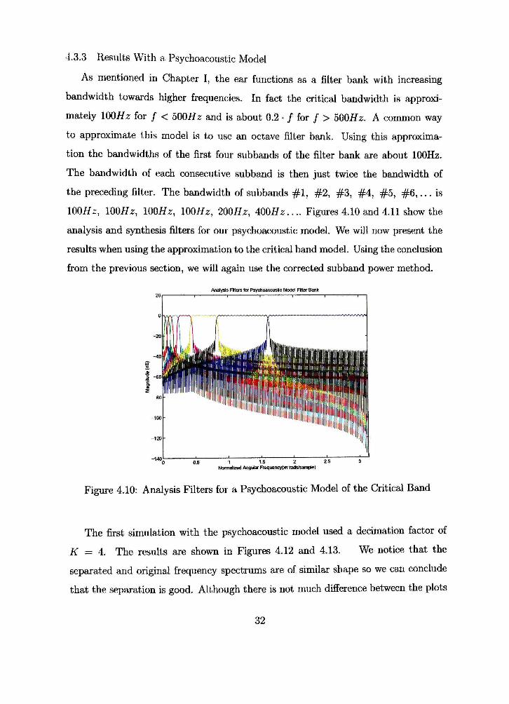
4.3.3 Results With a Psychoacoustic Model

As mentioned in Chapter I, the ear functions as a filter bank with increasing

bandwidth towards higher frequencies. In fact the critical bandwidth is approxi­

mately lOOHz for / < 500Hz and is about 0.2 • / for / > 500Hz. A common way

to approximate this model is to use an octave filter bank. Using this approxima­

tion the bandwidths of the first four subbands of the filter bank are about lOOHz.

The bandwidth of each consecutive subband is then just twice the bandwidth of

the preceding filter. The bandwidth of subbands # 1 , #2 , # 3 , #4 , # 5 , # 6 , . . . is

\OOHz, lOOHz, lOOHz, lOGHz, 200Hz, 400Hz.... Figiu-es 4.10 and 4.11 show the

analysis and synthesis filters for our psychoacoustic model. We will now present the

results when using the approximation to the critical band model. Using the conclusion

from the previous section, we will again use the corrected subband power method.

Analysis FiHe|.s for Psychoacoustic Model RIter Bank

1 15 2 25 Normalized /Vrgular Freqijenf;y<xii rads/sample)

Figure 4.10: Analysis Filters for a Psychoacoustic Model of the Critical Band

The first simulation with the psychoacoustic model used a decimation factor of

K = 4. The results are shown in Figures 4.12 and 4.13. We notice that the

separated and original frequency spectrums are of similar shape so we can conclude

that the separation is good. Although there is not much difference between the plots

32

Synthesis niters for Psychoecouslic Model FHter Bank

1 15 2 25 Noimalized Angrier Frequencytm rads/sample}

Figure 4.11: Synthesis Filters for a Psychoacoustic Model of the Critical Band

of the critical band method (Figures 4.12 and 4.13) versus the regular filter bank

method(4.8 and 4.9) there is a difference between the sound of the two methods.

The critical band method provides clearer signals when compared to the 64 channel

filter bank approach. Although not presented, without the subband power correction

aliasing becomes a noticeable problem even with the critical band approximation.

33

OHglnal Signal #1(blgllps_11.wav)

Figure 4.12: Separated Signal 1 using a Critical Band Approximation Filter Bank with K = 4 and subband Power Correction

Origmai Signal #2{pathok)gfcai_11.wav)

Figure 4.13: Separated Signal 2 using a Critical Band Approximation Filter Bank with K = 4 and subband Power Correction

34

CHAPTER V

SUMMARY AND CONCLUSION

This thesis aimed to improve the audibility of speech in noisy environments via

blind source separation. Chapter I introduced some basics of psychoacoustics and

explained how the human ear can be modelled as a filter bank with increasing band­

width. This critical band concept was incorporated in the filter bank design used for

this thesis.

Chapter II showed how to design prototype filters for low-delay modulated filter

banks. These prototypes were used to construct an estimation of the critical bands of

the ear. Chapter III introduced recent blind source separation techniques and theory.

The implementation of bfind source separation was covered in Chapter IV. This

chapter also showed how the subband power must be corrected to avoid aliasing.

Without this power correction the separated signals are noisy and even annoying.

We also showed in this chapter how the critical band approximation provided better

sound quafity of the separated signals than a regular filter bank.

In summary, this thesis showed how the incorporation of filter banks with current

blind source separation techniques may be a possibility for real world situations. By

dividing the incoming signals into subbands, we can divide the problem of source sep­

aration into smaUer parallel sub-tasks that can be possibly solved with less processing

time.

5.1 Future Work

Improvements stiU need to be made with the method presented in this thesis for

bfind source separation. The main improvements that needs to be made is a successful

way to group the separated signals in the subband domain. As mentioned in Chapter

IV, we currently use the original signals and compare them directly with the separated

signals in order to group them correctly. An algorithm that can possibly be used is

fundamental frequency estimation. Spectral information in speech is currently not

35

used in the technique described in this thesis. We can perhaps use the spectral

information to rearrange the separated signals correctly.

Another improvement needed for this algorithm is a process to minimize the alias­

ing introduced by the filter bank and the bfind source separation. Research must be

done to see if this can be overcome with filter bank design or in the BSS algorithm

itself

36

BIBLIOGRAPHY

[1] American speech-language-fiearing association, Worid Wide Web, 1999,

http://www.asha.org/hearing/disorders/prevalence_adults.cfin.

[2] A. Belouchrani, K. Abed-Maraim, J-F. Cardoso, and E. Moulines, A blind source separation technique using second-order statistics, IEEE Transactions on Signal Processing 45 (1997), no. 2, 434-444.

[3] J.-F. Cardoso, Blind beamforming for nan gaxissian signals, IEEE Trans, on Signal Processing 140 (1993), no. 6, 362-370.

[4] , Infomax and maximum likelihood for blind source separation., IEEE Signal Processing Letters 4 (1997), no. 4, 112-114.

[5] , Blind signal separation: Statistical principles., Proceedings of the IEEE 83 (1998), no. 10, 2009 - 2025.

[6] T.A. de Perez, Min Li, H. McAUister, and N.D. Black., Noise reduction and loudness compression in a wavelet modelling of the auditory system.. Proceedings of the 2000 Third IEEE International Caracas Conference on Devices, Circuits and Systems (2000), S l l / 1 - S l l /6 .

[7] John Durrant, Bases of hearing science, 2nd ed., WilUams k Wilkins, 1984.

[8] P. N. Heller, T. Karp, and T. Q. Nguyen, A general formulation of modulated filter banks, IEEE Trans, on Signal Processing 47 (1999), no. 4, 985-102.

[9] Aapo Hyvarinen and Erkki Oja, Independent component analysis: A tutorial., World Wide Web, 1999, http://www.cis.hut.fi/aapo/papers/IJCNN99_tutorialweb/IJCNN99.tutorial3.html.

[10] Alp. Kayabasi, Blind source separation, Tech. report, University of Maryland, Baltimore, 1997.

[11] T. Lee and R. Orghneister, Blind source separation of real-world signals, Proc. ICNN (Houston), 1997, pp. 2129-2135.

[12] Jerry M. Mendel, Tutorial on higher-order statistics (spectra) in signal processing and system theory: Theoretical results and some applications, Proceedings of the IEEE 79 (1991), no. 3, 278-305.

[13] Brian C.J. Moore, An introduction to the psychology of hearing, 2nd ed.. Aca­demic Press, San Diego, 1982.

[14] T. Q. Nguyen, Near-perfect-reconstruction pseudo-qmf banks, IEEE Transactions on Signal Processing 42 (1994), no. 1, 65-76.

37

[15] Thi Nguyen and C. Jutten, Blind source separation for convolutive mixtures, IEEE TVans. on Signal Processing 45 (1995), no. 2, 209-229.

[16] G. Strang and T. Nguyen., Wavelets and filter banks., Wellesley-Cambridge Press, Wellesley, MA, 1996.

[17] P. P. Vaidyanathan, Multirate systems and filter banks, Prentice HaU, 1993, pp. 354.

[18] E. Zwicker and H. Fasti, Psychoacoustics: Facts and models. Springer Verlag, Berlin, Germany, 1990.

38

PERMISSION TO COPY

In presenting this thesis in partial fulfillment of the requirements for a master's

degree at Texas Tech University or Texas Tech University Health Sciences Center, I

agree that the Library and my major department shall make it freely available for

research purposes. Permission to copy this thesis for scholarly purposes may be

granted by the Director of the Library or my major professor. It is understood that

any copying or publication of this thesis for financial gain shall not be allowed

without my further vmtten permission and diat any user may be liable for copyright

infringement.

Agree (Permission is granted.)

Disagree (Permission is not granted.)

Student Signature Date