1

Blind Separation of Speech Mixtures viaTime-Frequency Masking

Ozgur Yılmaz and Scott Rickard

Abstract—Binary time-frequency masks are a powerful tool forthe separation of sources from a single mixture. Perfect demix-ing via binary time-frequency masks is possible provided the time-frequency representations of the sources do not overlap, a con-dition we call W-disjoint orthogonality. We introduce here theconcept of approximate W-disjoint orthogonality and present ex-perimental results demonstrating the level of approximate W-disjoint orthogonality of speech in mixtures of various orders.The results demonstrate that ideal binary time-frequency masksexist which can separate several speech signals from one mix-ture. While determining these masks blindly from just one mix-ture is an open problem, we show that we can approximate theideal masks in the case where just two anechoic mixtures are pro-vided. Motivated by the maximum likelihood mixing parame-ter estimators, we define a power weighted two-dimensional his-togram constructed from the ratio of the time-frequency repre-sentations of the mixtures which is shown to have one peak foreach source with peak location corresponding to the relative at-tenuation and delay mixing parameters. The histogram is usedto create time-frequency masks which partition one mixture intothe original sources. Experimental results on speech mixtures ver-ify the technique. Example demixing results can be found online:http://www.princeton.edu/∼srickard/bss.html

I. INTRODUCTION

The goal in blind source separation is to determine the origi-nal sources given mixtures of those sources. When the numberof sources is greater than the number of mixtures, the problemis degenerate in that traditional matrix inversion demixing can-not be applied. However, when a representation of the sourcesexists such that the sources have disjoint support in that repre-sentation, it is possible to partition the support of the mixturesand obtain the original sources. One solution to the problem ofdegenerate demixing is thus to (1) determine an appropriate dis-joint representation of the sources and (2) determine the parti-tions in this representation which demix. In this paper, we showthat the Gabor expansion (i.e., the discrete short-time (or win-dowed) Fourier transform) is a good representation for demix-ing speech mixtures. Specifically, we show that partitions ofthe time-frequency lattice exist that can demix mixtures of upto ten speech signals from one mixture. Determining the parti-tion blindly from one mixture is an open problem, but, given asecond mixture, we describe a method for partitioning the time-frequency lattice which separates the sources.

Ozgur Yılmaz (oyilmaz@math.umd.edu) is with the Department of Mathe-matics, University of Maryland.

Scott Rickard (srickard@princeton.edu) is with the Program in Applied andComputational Mathematics, Princeton University and is also with SiemensCorporate Research in Princeton, NJ.

Submitted to IEEE Transactions on Signal Processing, November 4, 2002.

Formally, let S be the family of signals of interest. Typi-cally S will be some collection of square integrable bandlim-ited functions. Suppose there exists some linear transformationT : sj ∈ S 7→ Sj (where T maps the set S to another family offunctions) with the following properties:

(i) T is invertible on S (i.e., T−1(Ts) = T (T−1s) =s, ∀s ∈ S).

(ii) Λj ∩ Λk = ∅ for j 6= k, where Λj is the support of Sj ,i.e., Λj = supp Sj := λ : Sj(λ) 6= 0.

For example, we can consider the case where S is a collectionof square integrable functions with mutually disjoint supportsin the Fourier domain; any two functions s1 and s2 in S satisfys1(ω)s2(ω) = 0 for all ω, where sj denotes the Fourier trans-form of sj . Then if we define T on S as Ts := s, it is clear thatT satisfies (i) and (ii).

For any T with properties (i) and (ii), we can demix a mixturex1 of signals in S, x1(t) =

∑Nj=1 sj(t), via

sj = T−1(1ΛjTx1) (1)

where 1Λ is the indicator function of the set Λ. Going back toour example above, this corresponds to

sj = (1Λjx1) (2)

which is certainly true since the functions in S satisfy (ii). Here(1Λj

x1 ) denotes the inverse Fourier transform of 1Λjx1.

Suppose now that we have another mixture x2(t) =∑N

j=1 ajsj(t− δj), which is the case in anechoic environmentswhen we have two microphones. In the mixing, aj and δj arethe attenuation and delay parameters respectively correspond-ing to the j th source. Assume(iii) supp Ts(· − δ) = supp Ts for any s ∈ S, ∀|δ| < ∆, and(iv) there exist functions F and G such that aj =

F (Tx1(λ), Tx2(λ)) and δj = G(Tx1(λ), Tx2(λ)) forλ ∈ Λj for j = 1, . . . , N ,

where ∆ is the maximum possible delay between mixturesdue to the distance separating the sensors. Using (iii)and (iv), we can label each λ ∈ supp Tx1 with the pair(F (Tx1(λ), Tx2(λ)), G(Tx1(λ), Tx2(λ))), and Λj is exactlythe set of all points with the label (aj , δj). It follows that giventhe mixtures x1(t) and x2(t), we can demix via

sj = T−1(1ΛjTx1). (3)

Clearly, (iii) will be satisfied for the example above since theFourier transform of s(· − δ) will be just a modulated ver-sion of the Fourier transform of s and thus it will have the

2

same support as s. As to the existence of functions F andG, one can show that F (x1(ω), x2(ω)) = |x2(ω)/x1(ω)| andG(x1(ω), x2(ω)) = −1/ω^x2(ω)/x1(ω) where ^z denotesthe phase of the complex number z taken between −π and π,satisfies (iv). The above described F and G are the DUET at-tenuation and delay estimators for the special case where thewindowing function W ≡ 1. The DUET estimators are dis-cussed in Section III-A.

The general algorithm explained above mainly depends ontwo major points: (a) the existence of an invertible transforma-tion T that transforms the signals to a domain on which theyhave disjoint representations (properties (i), (ii), and (iii)), and(b) finding functions F and G that provide the means of la-beling on the transform domain (property (iv)). Note that inthe description above we required F and G to yield the exactmixing parameters. Although this is desired since the mixingparameters provide the perfect labels, and they can also be usedfor various other purposes (e.g., direction-of-arrival determina-tion), it is not necessary for the demixing algorithm to work.Some function that provides a unique labeling on the transformdomain is sufficient. Moreover, requirement (ii) that the trans-formation T is “disjoint” is very strong. In practice, one isusually more interested in transforms that satisfy (ii) in someapproximate sense. Therefore, we are interested in transformsthat result in sparse representations for the signals of interest.

There are many examples in the literature that do use thistype of approach with various choices of T for various mix-ing models and demixing methods[1–9]. The mixing model in[1–3, 5, 7, 8] is “instantaneous” (sources have different ampli-fications in different mixtures) while [4, 6, 9] use an anechoicmixing model (sources have different amplifications and timedelays in different mixtures). [1–3, 8] consider the time domainsampling operator as T . The general assumption in these is thatat any given time at most one source is non-zero. [4–7, 9] usethe short-time Fourier transform (STFT) operator as T . Condi-tion (ii) is satisfied in this case, at least approximately, becauseof the sparsity of the time-frequency representations of speechsignals. Empirical support for this can be found in [10], and amore extensive discussion is given in Section II-A. In principle,[1–9] all use some clustering algorithm for estimating the mix-ing parameters, although there are several different approachesto demixing. [1, 3, 4, 6–8] use a labeling scheme based on theestimated mixing parameters and thus demix in the above de-scribed way by creating binary masks in the transform domaincorresponding to each source. That is, given the mixtures x1

and x2, demixing is done by grouping the clusters of pointsin (Tx1, Tx2) space, although different techniques are used todetect these clusters. For example, [4, 6, 7] demix essentiallyby constructing binary time-frequency masks that partition thetime-frequency plane such that each partition corresponds tothe time-frequency points that “belong” to a particular source.The fact that such a mask exists has been observed also in [11]in the context of BSS of speech signals from one mixture, andin [12] in the context of source localization. In [2, 8, 9], thedemixing is done making additional assumptions on the statis-tical properties of the sources and using a maximum a posteri-ori (MAP) estimator. [5, 8] demix by assuming that the numberof sources active in the transform domain at any given point

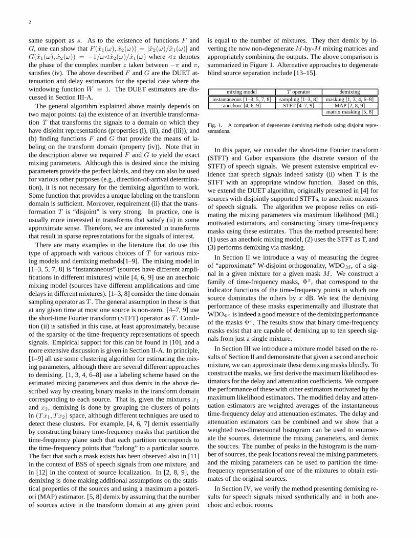
is equal to the number of mixtures. They then demix by in-verting the now non-degenerate M -by-M mixing matrices andappropriately combining the outputs. The above comparison issummarized in Figure 1. Alternative approaches to degenerateblind source separation include [13–15].

mixing model T operator demixing

instantaneous [1–3, 5, 7, 8] sampling [1–3, 8] masking [1, 3, 4, 6–8]anechoic [4, 6, 9] STFT [4–7, 9] MAP [2, 8, 9]

matrix masking [5, 8]

Fig. 1. A comparison of degenerate demixing methods using disjoint repre-sentations.

In this paper, we consider the short-time Fourier transform(STFT) and Gabor expansions (the discrete version of theSTFT) of speech signals. We present extensive empirical ev-idence that speech signals indeed satisfy (ii) when T is theSTFT with an appropriate window function. Based on this,we extend the DUET algorithm, originally presented in [4] forsources with disjointly supported STFTs, to anechoic mixturesof speech signals. The algorithm we propose relies on esti-mating the mixing parameters via maximum likelihood (ML)motivated estimators, and constructing binary time-frequencymasks using these estimates. Thus the method presented here:(1) uses an anechoic mixing model, (2) uses the STFT as T, and(3) performs demixing via masking.

In Section II we introduce a way of measuring the degreeof “approximate” W-disjoint orthogonality, WDOM , of a sig-nal in a given mixture for a given mask M . We construct afamily of time-frequency masks, Φx, that correspond to theindicator functions of the time-frequency points in which onesource dominates the others by x dB. We test the demixingperformance of these masks experimentally and illustrate thatWDOΦx is indeed a good measure of the demixing performanceof the masks Φx. The results show that binary time-frequencymasks exist that are capable of demixing up to ten speech sig-nals from just a single mixture.

In Section III we introduce a mixture model based on the re-sults of Section II and demonstrate that given a second anechoicmixture, we can approximate these demixing masks blindly. Toconstruct the masks, we first derive the maximum likelihood es-timators for the delay and attenuation coefficients. We comparethe performance of these with other estimators motivated by themaximum likelihood estimators. The modified delay and atten-uation estimators are weighted averages of the instantaneoustime-frequency delay and attenuation estimates. The delay andattenuation estimators can be combined and we show that aweighted two-dimensional histogram can be used to enumer-ate the sources, determine the mixing parameters, and demixthe sources. The number of peaks in the histogram is the num-ber of sources, the peak locations reveal the mixing parameters,and the mixing parameters can be used to partition the time-frequency representation of one of the mixtures to obtain esti-mates of the original sources.

In Section IV, we verify the method presenting demixing re-sults for speech signals mixed synthetically and in both ane-choic and echoic rooms.

3

II. W-DISJOINT ORTHOGONALITY

In this section, we focus on showing that binary time-frequency masks exist which are capable of separating multiplespeech signals from one mixture. Our goal is, given a mixture

x1(t) =

N∑

j=1

sj(t) (4)

of sources sj(t), j = 1, . . . , N , to recover the original sources.In order to accomplish this, we assume the sources are pairwiseW-disjoint orthogonal.

We call two functions s1 and s2 W-disjoint orthogonal (W-DO) if, for a given a window function W , the supports of thewindowed Fourier transforms of s1 and s2 are disjoint[4]. Thewindowed Fourier transform of sj is defined

F W (sj(·))(t, ω) =1√2π

∫ ∞

−∞

W (τ − t)sj(τ)e−iωτ dτ (5)

which we will refer to as sj(t, ω) where appropriate. For adetailed discussion of the properties of this transform consult[16]. The W-disjoint orthogonality assumption can be statedconcisely

s1(t, ω)s2(t, ω) = 0, ∀t, ω. (6)

The two limiting cases for W , namely W = 1 and W (t) =δ(t), result in interesting sets of W-DO signals. In the W = 1case, the t argument in (6) is irrelevant as the windowed Fouriertransform is simply the Fourier transform. The condition issatisfied by signals which are frequency disjoint, such as fre-quency division multiplexed signals. In the other extreme, sig-nals which are time disjoint such as time-division multiplexedsignals satisfy the condition. In general, for window functionswhich are localized in time and frequency, the W-disjoint or-thogonality condition is the goal of frequency-hopped multipleaccess systems. Indeed, the method presented here could beapplied to time-domain multiplexed, frequency domain multi-plexed, or frequency-hopped multiple access signals, however,in this paper we exclusively consider speech signals.

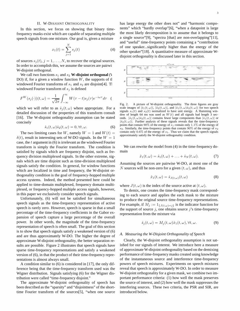
Unfortunately, (6) will not be satisfied for simultaneousspeech signals as the time-frequency representation of activespeech is rarely zero. However, speech is sparse in that a smallpercentage of the time-frequency coefficients in the Gabor ex-pansion of speech capture a large percentage of the overallpower. In other words, the magnitude of the time-frequencyrepresentation of speech is often small. The goal of this sectionis to show that speech signals satisfy a weakened version of (6)and are thus approximately W-DO. The higher the degree ofapproximate W-disjoint orthogonality, the better separation re-sults are possible. Figure 2 illustrates that speech signals havesparse time-frequency representations and satisfy a weakenedversion of (6), in that the product of their time-frequency repre-sentations is almost always small.

A condition similar to (6) is considered in [17], the only dif-ference being that the time-frequency transform used was theWigner distribution. Signals satisfying (6) for the Wigner dis-tribution were called “time-frequency disjoint.”

The approximate W-disjoint orthogonality of speech hasbeen described as the “sparsity” and “disjointness” of the short-time Fourier transform of the sources[5], “when one source

has large energy the other does not” and “harmonic compo-nents” which “hardly overlap”[6], “when a datapoint is largethe most likely decomposition is to assume that it belongs toa single source”[9], “spectra [that] are non-overlapping”[11],and “useful” time-frequency points containing a “contributionof one speaker...significantly higher than the energy of theother speaker”[18]. A quantitative measure of approximate W-disjoint orthogonality is discussed later in this section.

freq

|sW1

(t,ω)|

freq

|sW2

(t,ω)|

time

freq

|sW1

(t,ω)sW2

(t,ω)|

Fig. 2. A picture of W-disjoint orthogonality. The three figures are grayscale images of |s1(t, ω)|, |s2(t, ω)|, and |s1(t, ω)s2(t, ω)| for two speechsignals s1(t) and s2(t) normalized to have unit energy. A Hamming win-dow of length 64 ms was used as W (t) and all signals had length 3 sec-onds. |s1(t, ω)s2(t, ω)| contains fewer large components than |s1(t, ω)| or|s2(t, ω)|. Further analysis of these signals reveals that the time-frequencypoints that contain 90% of the energy of s1 contain only 1.1% of the energy ofs2. Similarly, the time-frequency points that contain 90% of the energy of s2

contain only 0.6% of the energy of s1. Thus we claim that the speech signalsapproximately satisfy the W-disjoint orthogonality condition.

We can rewrite the model from (4) in the time-frequency do-main

x1(t, ω) = s1(t, ω) + . . . + sN (t, ω). (7)

Assuming the sources are pairwise W-DO, at most one of theN sources will be non-zero for a given (t, ω), and thus

x1(t, ω) = sJ(t,ω)(t, ω) (8)

where J(t, ω) is the index of the source active at (t, ω).To demix, one creates the time-frequency mask correspond-

ing to each source and applies the each mask to the mixtureto produce the original source time-frequency representations.For example, if Mj := 1J(t,ω)=j is the indicator function forthe support of source j, one obtains source j’s time-frequencyrepresentation from the mixture via

sj(t, ω) = Mj(t, ω)x1(t, ω), ∀t, ω. (9)

A. Measuring the W-Disjoint Orthogonality of Speech

Clearly, the W-disjoint orthogonality assumption is not sat-isfied for our signals of interest. We introduce here a measureof approximate W-disjoint orthogonality based on the demixingperformance of time-frequency masks created using knowledgeof the instantaneous source and interference time-frequencypowers of speech mixtures. Experiments on speech mixturesreveal that speech is approximately W-DO. In order to measureW-disjoint orthogonality for a given mask, we combine two im-portant performance criteria: (1) how well the mask preservesthe source of interest, and (2) how well the mask suppresses theinterfering sources. These two criteria, the PSR and SIR, areintroduced below.

4

First, given a time-frequency mask M such that 0 ≤M(t, ω) ≤ 1 for all (t, ω), we define PSRM , the preserved-signal-ratio of the mask M as

PSRM =‖M(t, ω)sj(t, ω)‖2

‖sj(t, ω)‖2(10)

which measures the percentage of energy of source j remainingafter demixing using the mask. Note that PSRM ≤ 1 withPSRM = 1 only if supp Mj ⊆ supp M .

Now, we define

yj(t) =

N∑

k=1j 6=k

sk(t) (11)

so that yj(t) is the summation of the sources interfering withsource j. Then, we define the signal-to-interference ratio oftime-frequency mask M(t, ω)

SIRM =‖M(t, ω)sj(t, ω)‖2

‖M(t, ω)yj(t, ω)‖2(12)

which is the output signal-to-interference ratio after using themask to demix.

We now combine the PSRM and SIRM into one measure ofapproximate W-disjoint orthogonality. We propose the normal-ized difference between the signal energy maintained in mask-ing and the interference energy maintained in masking as ameasure of W-disjoint orthogonality:

WDOM =‖M(t, ω)sj(t, ω)‖2 − ‖M(t, ω)yj(t, ω)‖2

‖sj(t, ω)‖2(13)

= PSRM − PSRM/SIRM . (14)

Using the mask M(t, ω) = 1J(t,ω)=j, for signals which areW-DO we note that PSRM = 1, SIRM = ∞, and WDOM = 1.Moreover, WDOM = 1 implies that PSRM = 1, SIRM = ∞,and that (6) is satisfied. That is, WDOM = 1 implies that thesignals are W-DO.

Now we establish that binary time-frequency masks existwhich are capable of demixing speech signals from one mixtureand detail their performance in relation to the three presentedmeasures. Consider the following family of time-frequencymasks

Φxj (t, ω) =

1 20 log(|sj(t, ω)| / |yj(t, ω)|) ≥ x0 otherwise

(15)

which is the indicator function for the time-frequency pointswhere source j dominates the interference in the mixture by xdB. We will use PSRj(x) and SIRj(x) as shorthand for PSRΦx

j

and SIRΦxj, respectively.

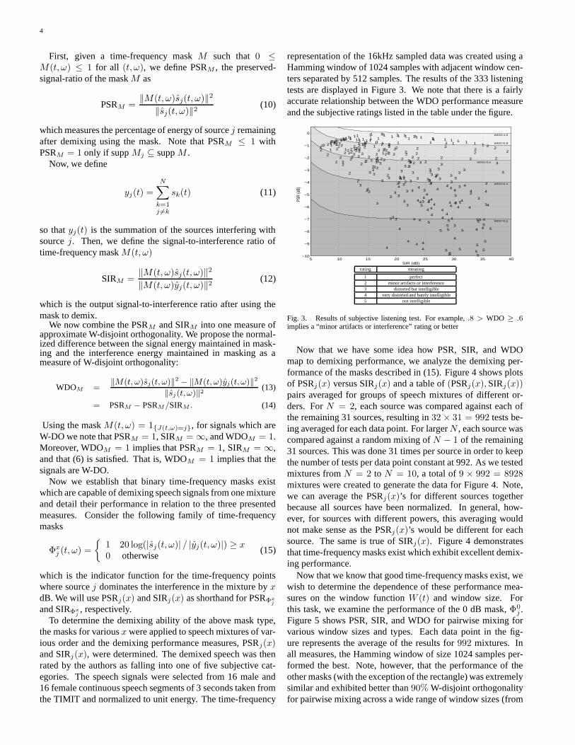
To determine the demixing ability of the above mask type,the masks for various x were applied to speech mixtures of var-ious order and the demixing performance measures, PSRj(x)and SIRj(x), were determined. The demixed speech was thenrated by the authors as falling into one of five subjective cat-egories. The speech signals were selected from 16 male and16 female continuous speech segments of 3 seconds taken fromthe TIMIT and normalized to unit energy. The time-frequency

representation of the 16kHz sampled data was created using aHamming window of 1024 samples with adjacent window cen-ters separated by 512 samples. The results of the 333 listeningtests are displayed in Figure 3. We note that there is a fairlyaccurate relationship between the WDO performance measureand the subjective ratings listed in the table under the figure.

5 10 15 20 25 30 35 40−10

−9

−8

−7

−6

−5

−4

−3

−2

−1

0WDO=1.0

WDO=0.8

WDO=0.6

WDO=0.4

WDO=0.2

1 1 11

2

2

3

11

2

2

3

3

4

1

2

2

3

4

4

5

11

2

3

3

4

5

1

2

2

2

3

4

5

2

2

2

3

3

4

1

2

3

3

4

2

2

3

3

4

5

2

2

3

4

5

5

1 1 11

2

2

3

11

1

2

3

3

4

1

1

1

2

3

3

1

1

2

2

3

3

4

2

2

2

3

3

4

5

2

2

2

3

4

5

5

2

2

2

3

1

2

3

3

4

2

3

3

4

1 1 11

1

2

2

11

1

2

2

3

3

11

2

2

3

4

4

22

2

3

4

4

5

1

1

2

3

3

4

5

2

2

3

3

4

5

1

2

2

3

4

2

2

2

3

4

5

2

3

3

4

5

5

1 1 1 1 1 1 1 1 1 1 1 1 1 22

2

1 1 1 11

22

22

22

33

3

3

3

11 1 1 1

22

2

22

3

33

4

4

4

1 1 1 1 22

2

22

3

3

3

4

4

4

5

11

2

22

2

2

3

3

4

4

44

5

55

11

12

2

2

3

3

3

4

4

4

5

5

22

22

2

3

3

33

4

4

4

4

5

22

22

2

3

3

3

33

4

4

22

2

2

2

2

3

3

4

4

PSR

(dB)

SIR (dB)

rating meaning

1 perfect2 minor artifacts or interference3 distorted but intelligible4 very distorted and barely intelligible5 not intelligible

Fig. 3. Results of subjective listening test. For example, .8 > WDO ≥ .6implies a “minor artifacts or interference” rating or better

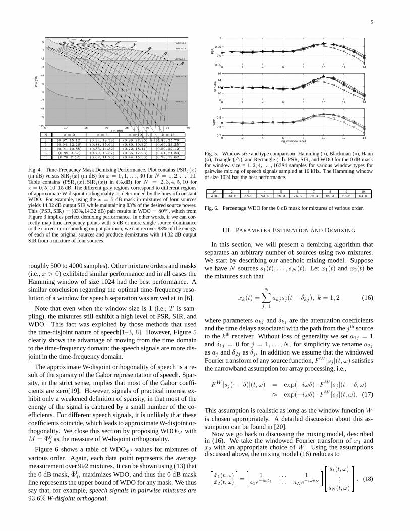
Now that we have some idea how PSR, SIR, and WDOmap to demixing performance, we analyze the demixing per-formance of the masks described in (15). Figure 4 shows plotsof PSRj(x) versus SIRj(x) and a table of (PSRj(x), SIRj(x))pairs averaged for groups of speech mixtures of different or-ders. For N = 2, each source was compared against each ofthe remaining 31 sources, resulting in 32 × 31 = 992 tests be-ing averaged for each data point. For larger N , each source wascompared against a random mixing of N − 1 of the remaining31 sources. This was done 31 times per source in order to keepthe number of tests per data point constant at 992. As we testedmixtures from N = 2 to N = 10, a total of 9 × 992 = 8928mixtures were created to generate the data for Figure 4. Note,we can average the PSRj(x)’s for different sources togetherbecause all sources have been normalized. In general, how-ever, for sources with different powers, this averaging wouldnot make sense as the PSRj(x)’s would be different for eachsource. The same is true of SIRj(x). Figure 4 demonstratesthat time-frequency masks exist which exhibit excellent demix-ing performance.

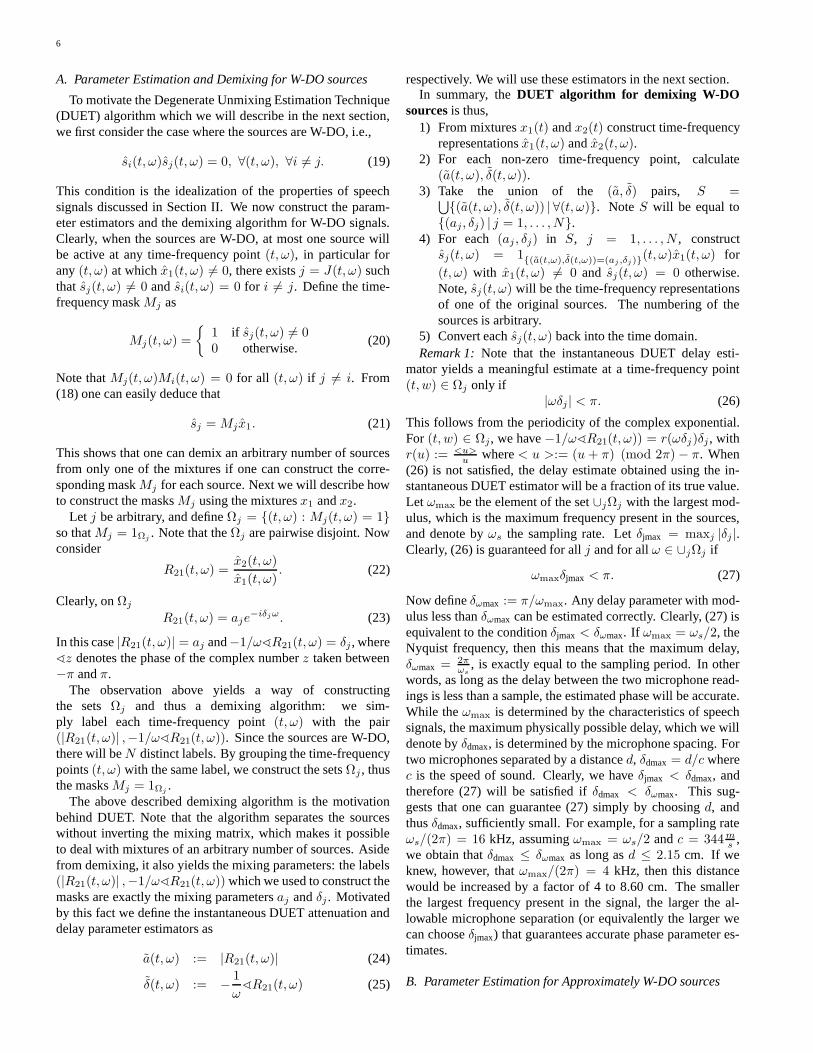
Now that we know that good time-frequency masks exist, wewish to determine the dependence of these performance mea-sures on the window function W (t) and window size. Forthis task, we examine the performance of the 0 dB mask, Φ0

j .Figure 5 shows PSR, SIR, and WDO for pairwise mixing forvarious window sizes and types. Each data point in the fig-ure represents the average of the results for 992 mixtures. Inall measures, the Hamming window of size 1024 samples per-formed the best. Note, however, that the performance of theother masks (with the exception of the rectangle) was extremelysimilar and exhibited better than 90% W-disjoint orthogonalityfor pairwise mixing across a wide range of window sizes (from

5

5 10 15 20 25 30 35 40−10

−9

−8

−7

−6

−5

−4

−3

−2

−1

0 WDO=1.0

WDO=0.8

WDO=0.6

WDO=0.4

WDO=0.2

PSR

(dB)

SIR (dB)

x=0

x=5

x=10

x=15

x=20

x=25

x=30

N=2N=3N=4N=5N=10

N x = 0 x = 5 x = 10 x = 15

2 (0.97, 15.12) (0.94, 18.39) (0.89, 21.96) (0.83, 25.76)

3 (0.94, 12.26) (0.88, 15.64) (0.80, 19.32) (0.69, 23.25)

4 (0.91, 10.88) (0.83, 14.32) (0.72, 18.11) (0.59, 22.12)

5 (0.89, 9.87) (0.79, 13.37) (0.65, 17.23) (0.51, 21.33)

10 (0.78, 7.52) (0.62, 11.23) (0.44, 15.33) (0.28, 19.62)

Fig. 4. Time-Frequency Mask Demixing Performance. Plot contains PSRj(x)(in dB) versus SIRj(x) (in dB) for x = 0, 1, . . . , 30 for N = 1, 2, . . . , 10.Table contains (PSRj(x), SIRj(x)) in (%,dB) for N = 2, 3, 4, 5, 10 forx = 0, 5, 10, 15 dB. The different gray regions correspond to different regionsof approximate W-disjoint orthogonality as determined by the lines of constantWDO. For example, using the x = 5 dB mask in mixtures of four sourcesyields 14.32 dB output SIR while maintaining 83% of the desired source power.This (PSR, SIR) = (83%,14.32 dB) pair results in WDO = 80%, which fromFigure 3 implies perfect demixing performance. In other words, if we can cor-rectly map time-frequency points with 5 dB or more single source dominanceto the correct corresponding output partition, we can recover 83% of the energyof each of the original sources and produce demixtures with 14.32 dB outputSIR from a mixture of four sources.

roughly 500 to 4000 samples). Other mixture orders and masks(i.e., x > 0) exhibited similar performance and in all cases theHamming window of size 1024 had the best performance. Asimilar conclusion regarding the optimal time-frequency reso-lution of a window for speech separation was arrived at in [6].

Note that even when the window size is 1 (i.e., T is sam-pling), the mixtures still exhibit a high level of PSR, SIR, andWDO. This fact was exploited by those methods that usedthe time-disjoint nature of speech[1–3, 8]. However, Figure 5clearly shows the advantage of moving from the time domainto the time-frequency domain: the speech signals are more dis-joint in the time-frequency domain.

The approximate W-disjoint orthogonality of speech is a re-sult of the sparsity of the Gabor representation of speech. Spar-sity, in the strict sense, implies that most of the Gabor coeffi-cients are zero[19]. However, signals of practical interest ex-hibit only a weakened definition of sparsity, in that most of theenergy of the signal is captured by a small number of the co-efficients. For different speech signals, it is unlikely that thesecoefficients coincide, which leads to approximate W-disjoint or-thogonality. We close this section by proposing WDOM withM = Φ0

j as the measure of W-disjoint orthogonality.

Figure 6 shows a table of WDOΦ0j

values for mixtures ofvarious order. Again, each data point represents the averagemeasurement over 992 mixtures. It can be shown using (13) thatthe 0 dB mask, Φ0

j , maximizes WDO, and thus the 0 dB maskline represents the upper bound of WDO for any mask. We thussay that, for example, speech signals in pairwise mixtures are93.6% W-disjoint orthogonal.

0 2 4 6 8 10 12 140.85

0.9

0.95

1

PS

R

0 2 4 6 8 10 12 148

10

12

14

16

SIR

(dB

)

0 2 4 6 8 10 12 140.7

0.8

0.9

1

log2(window size)

WD

O

Fig. 5. Window size and type comparison. Hamming (), Blackman (∗), Hann(), Triangle (4), and Rectangle (

). PSR, SIR, and WDO for the 0 dB mask

for window size = 1, 2, 4, . . . , 16384 samples for various window types forpairwise mixing of speech signals sampled at 16 kHz. The Hamming windowof size 1024 has the best performance.

N 2 3 4 5 6 7 8 9 10WDO 93.6 88.0 83.4 79.2 75.6 72.3 69.3 66.6 64.0

Fig. 6. Percentage WDO for the 0 dB mask for mixtures of various order.

III. PARAMETER ESTIMATION AND DEMIXING

In this section, we will present a demixing algorithm thatseparates an arbitrary number of sources using two mixtures.We start by describing our anechoic mixing model. Supposewe have N sources s1(t), . . . , sN (t). Let x1(t) and x2(t) bethe mixtures such that

xk(t) =

N∑

j=1

akjsj(t − δkj), k = 1, 2 (16)

where parameters akj and δkj are the attenuation coefficientsand the time delays associated with the path from the j th sourceto the kth receiver. Without loss of generality we set a1j = 1and δ1j = 0 for j = 1, . . . , N , for simplicity we rename a2j

as aj and δ2j as δj . In addition we assume that the windowedFourier transform of any source function, F W [sj ](t, ω) satisfiesthe narrowband assumption for array processing, i.e.,

F W [sj(· − δ)](t, ω) = exp(−iωδ) · F W [sj ](t − δ, ω)

≈ exp(−iωδ) · F W [sj ](t, ω). (17)

This assumption is realistic as long as the window function Wis chosen appropriately. A detailed discussion about this as-sumption can be found in [20].

Now we go back to discussing the mixing model, describedin (16). We take the windowed Fourier transform of x1 andx2 with an appropriate choice of W . Using the assumptionsdiscussed above, the mixing model (16) reduces to

x1(t, ω)x2(t, ω) =

1 . . . 1

a1e−iωδ1 . . . aNe−iωδN s1(t, ω)

...sN (t, ω)

. (18)

6

A. Parameter Estimation and Demixing for W-DO sources

To motivate the Degenerate Unmixing Estimation Technique(DUET) algorithm which we will describe in the next section,we first consider the case where the sources are W-DO, i.e.,

si(t, ω)sj(t, ω) = 0, ∀(t, ω), ∀i 6= j. (19)

This condition is the idealization of the properties of speechsignals discussed in Section II. We now construct the param-eter estimators and the demixing algorithm for W-DO signals.Clearly, when the sources are W-DO, at most one source willbe active at any time-frequency point (t, ω), in particular forany (t, ω) at which x1(t, ω) 6= 0, there exists j = J(t, ω) suchthat sj(t, ω) 6= 0 and si(t, ω) = 0 for i 6= j. Define the time-frequency mask Mj as

Mj(t, ω) =

1 if sj(t, ω) 6= 00 otherwise.

(20)

Note that Mj(t, ω)Mi(t, ω) = 0 for all (t, ω) if j 6= i. From(18) one can easily deduce that

sj = Mjx1. (21)

This shows that one can demix an arbitrary number of sourcesfrom only one of the mixtures if one can construct the corre-sponding mask Mj for each source. Next we will describe howto construct the masks Mj using the mixtures x1 and x2.

Let j be arbitrary, and define Ωj = (t, ω) : Mj(t, ω) = 1so that Mj = 1Ωj

. Note that the Ωj are pairwise disjoint. Nowconsider

R21(t, ω) =x2(t, ω)

x1(t, ω). (22)

Clearly, on Ωj

R21(t, ω) = aje−iδjω. (23)

In this case |R21(t, ω)| = aj and−1/ω^R21(t, ω) = δj , where^z denotes the phase of the complex number z taken between−π and π.

The observation above yields a way of constructingthe sets Ωj and thus a demixing algorithm: we sim-ply label each time-frequency point (t, ω) with the pair(|R21(t, ω)| ,−1/ω^R21(t, ω)). Since the sources are W-DO,there will be N distinct labels. By grouping the time-frequencypoints (t, ω) with the same label, we construct the sets Ωj , thusthe masks Mj = 1Ωj

.The above described demixing algorithm is the motivation

behind DUET. Note that the algorithm separates the sourceswithout inverting the mixing matrix, which makes it possibleto deal with mixtures of an arbitrary number of sources. Asidefrom demixing, it also yields the mixing parameters: the labels(|R21(t, ω)| ,−1/ω^R21(t, ω)) which we used to construct themasks are exactly the mixing parameters aj and δj . Motivatedby this fact we define the instantaneous DUET attenuation anddelay parameter estimators as

a(t, ω) := |R21(t, ω)| (24)

δ(t, ω) := − 1

ω^R21(t, ω) (25)

respectively. We will use these estimators in the next section.In summary, the DUET algorithm for demixing W-DO

sources is thus,1) From mixtures x1(t) and x2(t) construct time-frequency

representations x1(t, ω) and x2(t, ω).2) For each non-zero time-frequency point, calculate

(a(t, ω), δ(t, ω)).3) Take the union of the (a, δ) pairs, S =

⋃(a(t, ω), δ(t, ω)) | ∀(t, ω). Note S will be equal to(aj , δj) | j = 1, . . . , N.

4) For each (aj , δj) in S, j = 1, . . . , N , constructsj(t, ω) = 1(a(t,ω),δ(t,ω))=(aj ,δj)

(t, ω)x1(t, ω) for(t, ω) with x1(t, ω) 6= 0 and sj(t, ω) = 0 otherwise.Note, sj(t, ω) will be the time-frequency representationsof one of the original sources. The numbering of thesources is arbitrary.

5) Convert each sj(t, ω) back into the time domain.Remark 1: Note that the instantaneous DUET delay esti-

mator yields a meaningful estimate at a time-frequency point(t, w) ∈ Ωj only if

|ωδj | < π. (26)

This follows from the periodicity of the complex exponential.For (t, w) ∈ Ωj , we have −1/ω^R21(t, ω)) = r(ωδj)δj , withr(u) := <u>

u where < u >:= (u + π) (mod 2π) − π. When(26) is not satisfied, the delay estimate obtained using the in-stantaneous DUET estimator will be a fraction of its true value.Let ωmax be the element of the set ∪jΩj with the largest mod-ulus, which is the maximum frequency present in the sources,and denote by ωs the sampling rate. Let δjmax = maxj |δj |.Clearly, (26) is guaranteed for all j and for all ω ∈ ∪jΩj if

ωmaxδjmax < π. (27)

Now define δωmax := π/ωmax. Any delay parameter with mod-ulus less than δωmax can be estimated correctly. Clearly, (27) isequivalent to the condition δjmax < δωmax. If ωmax = ωs/2, theNyquist frequency, then this means that the maximum delay,δωmax = 2π

ωs, is exactly equal to the sampling period. In other

words, as long as the delay between the two microphone read-ings is less than a sample, the estimated phase will be accurate.While the ωmax is determined by the characteristics of speechsignals, the maximum physically possible delay, which we willdenote by δdmax, is determined by the microphone spacing. Fortwo microphones separated by a distance d, δdmax = d/c wherec is the speed of sound. Clearly, we have δjmax < δdmax, andtherefore (27) will be satisfied if δdmax < δωmax. This sug-gests that one can guarantee (27) simply by choosing d, andthus δdmax, sufficiently small. For example, for a sampling rateωs/(2π) = 16 kHz, assuming ωmax = ωs/2 and c = 344m

s ,we obtain that δdmax ≤ δωmax as long as d ≤ 2.15 cm. If weknew, however, that ωmax/(2π) = 4 kHz, then this distancewould be increased by a factor of 4 to 8.60 cm. The smallerthe largest frequency present in the signal, the larger the al-lowable microphone separation (or equivalently the larger wecan choose δjmax) that guarantees accurate phase parameter es-timates.

B. Parameter Estimation for Approximately W-DO sources

7

1) Maximum Likelihood Estimators for Delay and Attenu-ation Coefficients: In Section II, we have illustrated that thetime-frequency representations of speech signals are sparse,and one can indeed recover a speech signal from one mixture ofan arbitrary number of sources if one can construct an appropri-ate time-frequency mask. This suggests that a weakened W-DOcondition holds for speech signals: if at a time-frequency pointone of the sources has considerable power, the contribution ofall the other sources at that time-frequency point is likely to besmall. This observation is the key to the demixing algorithm wepropose in this section. First we shall discuss how to estimatethe mixing parameters.

Instead of the continuous windowed Fourier transform, weuse the equivalent discrete counterpart1

sj [k, l] = sj(kt0, lω0) (28)

where t0 and ω0 are the time-frequency lattice spacing parame-ters.

We will say that sj is dominant at [k, l] if |sj [k, l]| ≥|yj [k, l]|, where yj is as in (11). Note, the 0 dB mask, Φ0

j , in(15) is the indicator function for the dominant time-frequencypoints for source j. Let us concentrate on one source, say s.Let Ω be the set of time-frequency points [k, l] at which s isdominant in the sense described above. On Ω, we model themixtures x1 and x2 as follows:

x1[k, l] = s[k, l] + n1[k, l]

x2[k, l] = ae−iδlω0 s[k, l] + n2[k, l] (29)

where n1 and n2 are i.i.d. white complex Gaussian noise withzero-mean and variance σ2. Here n1 and n2 model the contri-butions of other sources at the time-frequency points where s isthe dominant source. We model the interfering sources as inde-pendent Gaussian noise in order to obtain simple closed-formsource and mixing parameter estimators. In reality, the interfer-ence in the different mixtures will be correlated and may not beGaussian distributed. For the model in (29), we want to employa ML estimate to find the parameter pair (a, δ) ∈ R

2 as wellas s[k, l] that maximize P (x1, x2|a, δ). To that goal, we definethe likelihood , L0, of (s, a, δ), where s = (s[k, l])(k,l)∈Λ witheach s[k, l] ∈ C for some index set Λ ⊂ Z2, given the datax1[k, l] and x2[k, l], by

L0(s, a, δ):=p(x1, x2|s, a, δ)

= (k,l)∈Λ

fN1,N2 (x1[k, l] − s[k, l], x2[k, l] − ae−iδlω0 s[k, l])

=C exp − 1

2σ2 (k,l)∈Λ

|x1[k, l] − s[k, l]|2 + x2[k, l] − ae−iδlω0 s[k, l] 2 (30)

where xi = (xi[k, l])(k,l)∈Λ. The last equality holds becausewe assume i.i.d. complex Gaussian noise. Clearly, maximizingL0 is equivalent to maximizing

L(s, a, δ) :=− (k,l)∈Λ

|x1[k, l] − s[k, l]|2+ x2[k, l] − ae−iδlω0 s[k, l]

2 .

(31)

1The equivalence is nontrivial and only true for appropriately chosen windowfunctions W with sufficiently small t0 and ω0. An illustrative discussion canbe found in [16].

For this purpose, we want to solve the equations ∂L∂α[k,l] = 0,

∂L∂β[k,l] = 0 for all (k, l) ∈ Λ, ∂L

∂a = 0 and ∂L∂δ = 0 simul-

taneously, where α[k, l] and β[k, l] denote the real and imagi-nary parts of s[k, l] respectively. We start with ∂L

∂α[k,l] . For any(k, l) ∈ Λ, we have

∂L

∂α[k, l]=

∂

∂α[k, l]

(

|x1[k, l]− α[k, l] − iβ[k, l]|2 +

∣

∣x2[k, l] − ae−iδlω0(α[k, l] + iβ[k, l])∣

∣

2)

.(32)

We solve then ∂L∂α[k,l]

∣

∣

∣

α[k,l]=α∗[k,l]= 0 for α∗[k, l] and obtain

α∗[k, l] = Re

x1[k, l] + aeiδlω0 x2[k, l]

1 + a2

. (33)

Similarly, solving ∂L∂β[k,l]

∣

∣

∣

β[k,l]=β∗[k,l]= 0 for β∗[k, l] yields

β∗[k, l] = Im

x1[k, l] + aeiδlω0 x2[k, l]

1 + a2

(34)

which we combine with (33) to get the ML estimate s∗ for s:

s∗[k, l] =

x1[k, l] + aeiδlω0 x2[k, l]

1 + a2. (35)

Next, we consider ∂L∂δ . We have

∂L

∂δ=

∂

∂δ

∑

(k,l)∈Λ

∣

∣x2[k, l] − ae−iδlω0 s[k, l]∣

∣

2

= 2a∑

(k,l)∈Λ

lω0Im

x2[k, l]s[k, l]eiδlω0

. (36)

We now plug in s[k, l] = s∗[k, l] in (36), which yields

∂L

∂δ=

2a

1 + a2

∑

(k,l)∈Λ

lω0 |x1[k, l]|2 Im

R21[k, l]eiδlω0

=2a

1 + a2

∑

(k,l)∈Λ

lω0 |x1[k, l]x2[k, l]| sin(^R21[k, l] + δlω0)(37)

where R21[k, l] := x2[k,l]x1[k,l] . We define the instantaneous DUET

delay estimate for the parameter δ, the discrete version of (25)

δ[k, l] = − 1

lω0^R21[k, l]. (38)

and for convenience, define δ[k, l] = 0 if x1[k, l] = 0or x2[k, l] = 0. We assume that |^R21[k, l] + δlω0| =∣

∣

∣lω0(δ − δ[k, l])

∣

∣

∣is small which is reasonable because we are

considering only the [k, l] where s is dominant and we make theapproximation

sin(^R21[k, l] + δlω0) ≈ ^R21[k, l] + δlω0. (39)

After plugging (39) into (37), we solve the equation ∂L∂δ

∣

∣

δ=δ∗=

0 for δ∗ and obtain

δ∗ =

∑

(k,l)∈Λ δ[k, l]l2ω20 |x1[k, l]x2[k, l]|

∑

(k,l)∈Λ l2ω20 |x1[k, l]x2[k, l]| . (40)

8

Note that δ∗, the ML estimate for the parameter δ, is a weightedaverage of the instantaneous DUET delay estimates, with eachestimate weighted by the product magnitude of the mixtures aswell as (lω0)

2. We also observe that the ML estimate δ∗ doesnot depend on the attenuation parameter a.

Finally, we will solve the equation ∂L∂a

∣

∣

a=a∗for a∗. We have

∂L

∂a=

∂

∂a

∑

(k,l)∈Λ

∣

∣x2[k, l] − ae−iδlω0 s[k, l]∣

∣

2

=∑

(k,l)∈Λ

2a |s[k, l]|2 − 2Re

x2[k, l]s[k, l]eiδlω0

. (41)

After setting s[k, l] = s∗[k, l] and some algebra we get

a∗ − 1

a∗=

∑

(k,l)∈Λ |x1[k, l]x2[k, l]| (a[k, l] − 1/a[k, l])∑

(k,l)∈Λ Re

x2[k, l]x1[k, l]eiδ∗lω0

(42)where

a[k, l] = |R21[k, l]| (43)

is the discrete version of the instantaneous DUET attenua-tion estimate (24). For convenience, we define a[k, l] = 1 ifx1[k, l] = 0 or x2[k, l] = 0.

The estimate for a∗ − 1a∗

is symmetric in x1 and x2: swap-ping the mixture labels will only result in a sign change of thisquantity (i.e., (1/a) − (1/(1/a)) = −(a − 1/a)). In the orig-inal presentation of DUET [4], the logarithm of the attenua-tion estimates was used solely because it has the same property(i.e.,log(1/a) = − log(a)). However, motivated by its appear-ance in the ML estimator (42), we will replace the role of thelogarithm with the DUET symmetric attenuation estimator de-fined as a[k, l]− 1/a[k, l].

Remark 2: Although the estimate given in (42) is not aweighted average, it is interesting to note that if we replace δ∗ in(42) with the instantaneous DUET phase estimates δ[k, l] whichsatisfy

eiδ[k,l]lω0 =R21[k, l]

|R21[k, l]| (44)

we obtain that

Re

x2[k, l]x1[k, l]eiδ[k,l]lω0

= |x1[k, l]x2[k, l]| (45)

and in this case, (42) becomes a weighted average of a[k, l] −1/a[k, l].

2) Experimental Evaluation of the ML Estimator: In thissection, we experimentally evaluate the ML estimators as wellas other estimators motivated by the previous section. In ordersimulate mixtures, we use the model in (29) and adjust the noisepower to model the different number of interfering sources. Themodel in (29) is valid for the dominant time-frequency pointsof one source s. In order to determine the set of dominanttime-frequency points Λ, a speech signal taken from the TIMITdatabase was compared to a random mixture of 1, 2, 4, or 9TIMIT speech signals to model the N = 2, 3, 5, 10 mixture or-ders, and in each case, the time-frequency points correspondingto the 0-dB mask were selected. The mixtures of interfering

sources were only used to determine Λ and were discarded af-ter the dominant time-frequency points were identified. In orderto simulate the presence of interfering sources, i.i.d. Gaussianwhite noise was added to the dominant time-frequency pointsof source s on both channels. The added noise was amplifiedto produce a 15.12 dB, 12.26 dB, 9.87 dB, or 7.52 dB SNR soas to model mixing of order N = 2, 3, 5, or 10, respectively.These SNR’s were selected to model different mixture ordersbecause they match the average SIR’s for the 0-dB mask fromFigure 4. That is, 15.12 dB, 12.26 dB, 9.87 dB, and 7.52 dBare the expected SIR’s after applying the 0-dB mask to mix-tures of order N = 2, 3, 5, and 10, and thus in order to modelthese mixture orders for the dominant time-frequency points ofone source, we add noise to one source to produce the corre-sponding SNR’s. Note that the dominate time-frequency pointsare precisely the support of the source’s 0 dB mask. Thus theperformance of the estimator evaluated with this model at theseSNR’s should approximate the true performance of the estima-tor in speech mixtures of order N = 2, 3, 5, and 10. All re-sults in the remainder of this section will be obtained using thismodel.

We choose to experimentally evaluate the estimators usingthe model as described above as opposed to creating syntheticmixtures of multiple speech signals because we (1) wanted toprevent the results from depending on the specific choice ofmixing parameters of the interfering sources and (2) wantedto evaluate the estimators using the model that motivatedthem. The disadvantage of modeling the presence of interferingsources in this way is that the interference should be correlatedand this correlation is lost when the interference is modeled asindependent noise. Our desire in this section is to explore thequalitative performance of a family of estimators to motivatethe demixing algorithm, and modeling the interference as noiseis sufficient for this purpose.

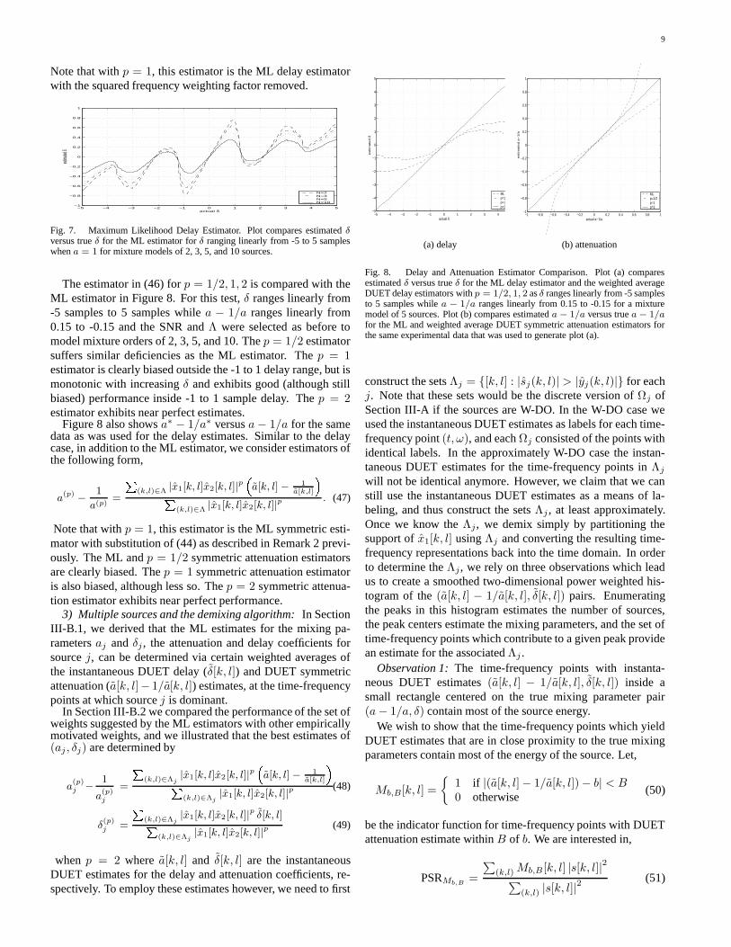
Figure 7 shows the ML estimate δ∗ from (40) versus δ as δranges linearly from -5 samples to 5 samples with a = 1. Wecan see that the ML delay estimator exhibits bad performanceoutside the -1 to 1 sample range, and biased performance in-side this range. The bad performance for larger delays is due tothe phase wrap around problem discussed in Remark 1 in Sec-tion III-B.1. The squared frequency weighting factor in the MLdelay estimator accentuates this problem. In addition, such afrequency weighting would make signals with higher frequencycontent have higher likelihood estimates of their delay param-eters. In the next sections, we will be using these weightingsto construct weighted histograms for source separation and it isundesirable to assign more likelihood to one set of parameterssimply because their associated source contains higher frequen-cies. While methods for unwrapping the phase do exist, thesemethods are inappropriate for our purposes as different sourcesmay be active from one frequency to the next. In order to see ifwe could reduce the bias, eliminate the wrap-around effect, andremove the high frequency weighting, we removed the squaredfrequency weighting factor in the ML delay estimator and con-sidered estimators of the following form

δ(p)j =

∑

(k,l)∈Λ |x1[k, l]x2[k, l]|p δ[k, l]∑

(k,l)∈Λ |x1[k, l]x2[k, l]|p . (46)

9

Note that with p = 1, this estimator is the ML delay estimatorwith the squared frequency weighting factor removed.

−5 −4 −3 −2 −1 0 1 2 3 4 5−1

−0.8

−0.6

−0.4

−0.2

0

0.2

0.4

0.6

0.8

1

actual δ

estima

ted δ

N=2 N=3 N=5 N=10

Fig. 7. Maximum Likelihood Delay Estimator. Plot compares estimated δversus true δ for the ML estimator for δ ranging linearly from -5 to 5 sampleswhen a = 1 for mixture models of 2, 3, 5, and 10 sources.

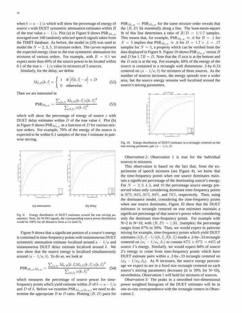
The estimator in (46) for p = 1/2, 1, 2 is compared with theML estimator in Figure 8. For this test, δ ranges linearly from-5 samples to 5 samples while a − 1/a ranges linearly from0.15 to -0.15 and the SNR and Λ were selected as before tomodel mixture orders of 2, 3, 5, and 10. The p = 1/2 estimatorsuffers similar deficiencies as the ML estimator. The p = 1estimator is clearly biased outside the -1 to 1 delay range, but ismonotonic with increasing δ and exhibits good (although stillbiased) performance inside -1 to 1 sample delay. The p = 2estimator exhibits near perfect estimates.

Figure 8 also shows a∗ − 1/a∗ versus a − 1/a for the samedata as was used for the delay estimates. Similar to the delaycase, in addition to the ML estimator, we consider estimators ofthe following form,

a(p) −1

a(p)= (k,l)∈Λ |x1[k, l]x2[k, l]|p a[k, l] − 1

a[k,l] (k,l)∈Λ |x1[k, l]x2[k, l]|p. (47)

Note that with p = 1, this estimator is the ML symmetric esti-mator with substitution of (44) as described in Remark 2 previ-ously. The ML and p = 1/2 symmetric attenuation estimatorsare clearly biased. The p = 1 symmetric attenuation estimatoris also biased, although less so. The p = 2 symmetric attenua-tion estimator exhibits near perfect performance.

3) Multiple sources and the demixing algorithm: In SectionIII-B.1, we derived that the ML estimates for the mixing pa-rameters aj and δj , the attenuation and delay coefficients forsource j, can be determined via certain weighted averages ofthe instantaneous DUET delay (δ[k, l]) and DUET symmetricattenuation (a[k, l]− 1/a[k, l]) estimates, at the time-frequencypoints at which source j is dominant.

In Section III-B.2 we compared the performance of the set ofweights suggested by the ML estimators with other empiricallymotivated weights, and we illustrated that the best estimates of(aj , δj) are determined by

a(p)j −

1

a(p)j

= (k,l)∈Λj|x1[k, l]x2[k, l]|p a[k, l] − 1

a[k,l] (k,l)∈Λj|x1[k, l]x2[k, l]|p

(48)

δ(p)j = (k,l)∈Λj

|x1[k, l]x2[k, l]|p δ[k, l] (k,l)∈Λj|x1[k, l]x2[k, l]|p

(49)

when p = 2 where a[k, l] and δ[k, l] are the instantaneousDUET estimates for the delay and attenuation coefficients, re-spectively. To employ these estimates however, we need to first

−5 −4 −3 −2 −1 0 1 2 3 4 5−5

−4

−3

−2

−1

0

1

2

3

4

5

actual δ

estim

ate

d δ

ML p=1/2p=1 p=2

(a) delay

−1 −0.8 −0.6 −0.4 −0.2 0 0.2 0.4 0.6 0.8 1−1

−0.8

−0.6

−0.4

−0.2

0

0.2

0.4

0.6

0.8

1

actual a−1/a

estim

ate

d a

−1

/a

ML p=1/2p=1 p=2

(b) attenuation

Fig. 8. Delay and Attenuation Estimator Comparison. Plot (a) comparesestimated δ versus true δ for the ML delay estimator and the weighted averageDUET delay estimators with p = 1/2, 1, 2 as δ ranges linearly from -5 samplesto 5 samples while a − 1/a ranges linearly from 0.15 to -0.15 for a mixturemodel of 5 sources. Plot (b) compares estimated a − 1/a versus true a − 1/afor the ML and weighted average DUET symmetric attenuation estimators forthe same experimental data that was used to generate plot (a).

construct the sets Λj = [k, l] : |sj(k, l)| > |yj(k, l)| for eachj. Note that these sets would be the discrete version of Ωj ofSection III-A if the sources are W-DO. In the W-DO case weused the instantaneous DUET estimates as labels for each time-frequency point (t, ω), and each Ωj consisted of the points withidentical labels. In the approximately W-DO case the instan-taneous DUET estimates for the time-frequency points in Λj

will not be identical anymore. However, we claim that we canstill use the instantaneous DUET estimates as a means of la-beling, and thus construct the sets Λj , at least approximately.Once we know the Λj , we demix simply by partitioning thesupport of x1[k, l] using Λj and converting the resulting time-frequency representations back into the time domain. In orderto determine the Λj , we rely on three observations which leadus to create a smoothed two-dimensional power weighted his-togram of the (a[k, l] − 1/a[k, l], δ[k, l]) pairs. Enumeratingthe peaks in this histogram estimates the number of sources,the peak centers estimate the mixing parameters, and the set oftime-frequency points which contribute to a given peak providean estimate for the associated Λj .

Observation 1: The time-frequency points with instanta-neous DUET estimates (a[k, l] − 1/a[k, l], δ[k, l]) inside asmall rectangle centered on the true mixing parameter pair(a − 1/a, δ) contain most of the source energy.

We wish to show that the time-frequency points which yieldDUET estimates that are in close proximity to the true mixingparameters contain most of the energy of the source. Let,

Mb,B[k, l] =

1 if |(a[k, l] − 1/a[k, l]) − b| < B0 otherwise

(50)

be the indicator function for time-frequency points with DUETattenuation estimate within B of b. We are interested in,

PSRMb,B=

∑

(k,l) Mb,B [k, l] |s[k, l]|2∑

(k,l) |s[k, l]|2(51)

10

when b = a− 1/a which will show the percentage of energy ofsource s with DUET symmetric attenuation estimates within Bof the true value a − 1/a. Plot (a) in Figure 9 shows PSRMb,B

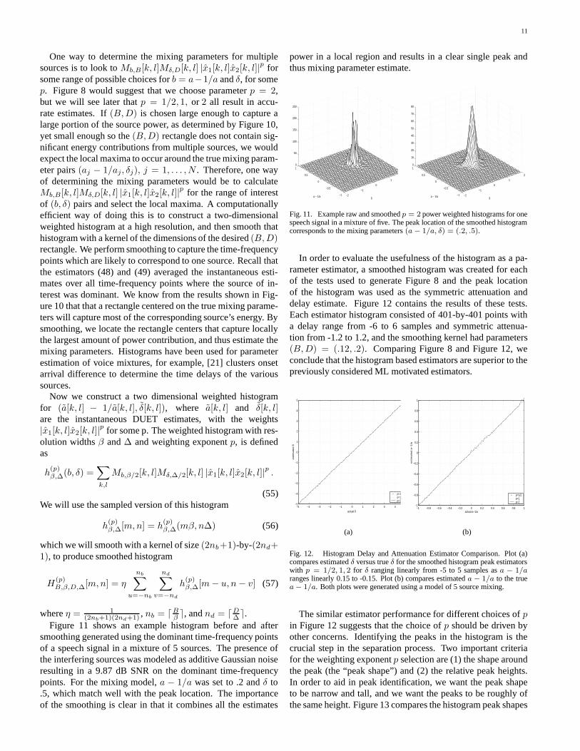
averaged over 100 randomly selected speech signals taken fromthe TIMIT database. As before, the model in (29) was used tomodel the N = 2, 3, 5, 10 mixture orders. The curves representthe expected energy close to the true symmetric attenuation formixtures of various orders. For example, with B = 0.1 weexpect more than 60% of the source power to be located within0.1 of the true a − 1/a value in mixtures of 5 sources.

Similarly, for the delay, we define

Md,D[k, l] =

1 if∣

∣

∣δ[k, l] − d∣

∣

∣ < D

0 otherwise.(52)

Then we are interested in

PSRMδ,D=

∑

(k,l) Mδ,D[k, l] |s[k, l]|2∑

(k,l) |s[k, l]|2(53)

which will show the percentage of energy of source s withDUET delay estimates within D of the true value δ. Plot (b)in Figure 9 shows PSRMδ,D

as a function of D for various mix-ture orders. For example, 70% of the energy of the source isexpected to be within 0.1 samples of the true δ estimate in pair-wise mixing.

0 0.1 0.2 0.3 0.4 0.5 0.60

0.1

0.2

0.3

0.4

0.5

0.6

0.7

0.8

0.9

1

B, the distance from b = a − 1/a

% s

ou

rce

en

erg

y w

ith

in B

of b

N=2 N=3 N=5 N=10

(a) attenuation

0 0.1 0.2 0.3 0.4 0.5 0.6 0.7 0.8 0.9 10

0.1

0.2

0.3

0.4

0.5

0.6

0.7

0.8

0.9

1

D, the distance from δ

% s

ou

rce

en

erg

y w

ith

in D

of

δ

N=2 N=3 N=5 N=10

(b) delay

Fig. 9. Energy distribution of DUET estimates around the true mixing pa-rameters. Note, for W-DO signals, the corresponding source power distributionwould be 100% for all distances from a-1/a (and δ).

Figure 9 shows that a significant portion of a source’s energyis contained in time-frequency points with instantaneous DUETsymmetric attenuation estimate localized around a − 1/a andinstantaneous DUET delay estimate localized around δ. Wenow show that the source energy is localized simultaneouslyaround (a − 1/a, δ). To do so, we look at

PSRMb,BMδ,D=

∑

(k,l) Mb,B[k, l]Mδ,D[k, l] |s[k, l]|2∑

(k,l) |s[k, l]|2(54)

which measures the percentage of source power for time-frequency points which yield estimate within B of b = a− 1/aand D of δ. Before we examine PSRMb,BMδ,D

, we need to de-termine the appropriate B to D ratio. Plotting (B, D) pairs for

PSRMb,B= PSRMδ,D

for the same mixture order reveals thatthe (B, D) lie essentially along a line. The least-mean-squarefit of this line determines a ratio of B/D = 1/1.7 samples.This means that, for example, PSRMb,B

≈ .6 for B = .1 forN = 5 implies that PSRMδ,D

≈ .6 for D = 1.7 × .1 = .17samples for N = 5, a property which can be verified from thedata displayed in Figure 9. Figure 10 shows PSRMB,D

versus Band D for 1.7B = D. Note that the B axis is at the bottom andthe D axis is at the top. For example, 60% of the energy of thesource is contained in a rectangle with dimensions .2-by-0.33centered on (a − 1/a, δ) for mixtures of three sources. As thenumber of sources increases, the energy spreads over a widerarea, but the source energy remains well localized around thesource’s mixing parameters.

0 0.1 0.2 0.3 0.4 0.5 0.60

0.1

0.2

0.3

0.4

0.5

0.6

0.7

0.8

0.9

1

B, the distance from b = a − 1/a

% s

ou

rce

en

erg

y w

ithin

B o

f b

an

d D

of

δ

0.00 0.17 0.33 0.50 0.67 0.84 1.00D, the distance from δ

N=2 N=3 N=5 N=10

Fig. 10. Energy distribution of DUET estimates in a rectangle centered on thetrue mixing parameter pair (a − 1/a, δ).

Observation 2: Observation 1 is true for the individualsources in mixtures.

This observation is based on the fact that, from the ex-periments of speech mixtures (see Figure 4), we know thatthe time-frequency points when one source dominates main-tain a significant percentage of the dominating source’s energy.For N = 2, 3, 4, 5, and 10 the percentage source energy pre-served when only considering dominant time-frequency pointsis 97%, 94%, 91%, 89%, and 78%, respectively. Then, usingthe dominance model, considering the time-frequency pointswhen one source dominates, Figure 10 show that the DUETestimates in rectangle centered on true estimates maintain asignificant percentage of that source’s power when consideringonly the dominant time-frequency points. For example withN=2 to N=10, with (B, D) = (.33, .2samples) the percentageranges from 87% to 50%. Thus, we would expect in pairwisemixing for example, time-frequency points which yield DUETestimates (a[k, l]−1/a[k, l], δ[k, l]) inside a .2-by-.33 rectanglecentered on (a1 − 1/a1, δ1) to contain 87% × 97% = 84% ofsource 1’s energy. Similarly, we would expect 84% of source2’s energy to come from time-frequency points which haveDUET estimate pairs within a .2-by-.33 rectangle centered on(a2 − 1/a2, δ2). As N increases, the source energy percent-age we expect to see in a fixed size rectangle centered on eachsource’s mixing parameters decreases (it is 39% for N=10),nevertheless, Observation 1 will hold for mixtures of sources.

Observation 3: The peaks in a smoothed two-dimensionalpower weighted histogram of the DUET estimates will be inone-to-one correspondence with the rectangle centers in Obser-vation 2.

11

One way to determine the mixing parameters for multiplesources is to look to Mb,B[k, l]Mδ,D[k, l] |x1[k, l]x2[k, l]|p forsome range of possible choices for b = a−1/a and δ, for somep. Figure 8 would suggest that we choose parameter p = 2,but we will see later that p = 1/2, 1, or 2 all result in accu-rate estimates. If (B, D) is chosen large enough to capture alarge portion of the source power, as determined by Figure 10,yet small enough so the (B, D) rectangle does not contain sig-nificant energy contributions from multiple sources, we wouldexpect the local maxima to occur around the true mixing param-eter pairs (aj − 1/aj , δj), j = 1, . . . , N . Therefore, one wayof determining the mixing parameters would be to calculateMb,B [k, l]Mδ,D[k, l] |x1[k, l]x2[k, l]|p for the range of interestof (b, δ) pairs and select the local maxima. A computationallyefficient way of doing this is to construct a two-dimensionalweighted histogram at a high resolution, and then smooth thathistogram with a kernel of the dimensions of the desired (B, D)rectangle. We perform smoothing to capture the time-frequencypoints which are likely to correspond to one source. Recall thatthe estimators (48) and (49) averaged the instantaneous esti-mates over all time-frequency points where the source of in-terest was dominant. We know from the results shown in Fig-ure 10 that that a rectangle centered on the true mixing parame-ters will capture most of the corresponding source’s energy. Bysmoothing, we locate the rectangle centers that capture locallythe largest amount of power contribution, and thus estimate themixing parameters. Histograms have been used for parameterestimation of voice mixtures, for example, [21] clusters onsetarrival difference to determine the time delays of the varioussources.

Now we construct a two dimensional weighted histogramfor (a[k, l] − 1/a[k, l], δ[k, l]), where a[k, l] and δ[k, l]are the instantaneous DUET estimates, with the weights|x1[k, l]x2[k, l]|p for some p. The weighted histogram with res-olution widths β and ∆ and weighting exponent p, is definedas

h(p)β,∆(b, δ) =

∑

k,l

Mb,β/2[k, l]Mδ,∆/2[k, l] |x1[k, l]x2[k, l]|p .

(55)We will use the sampled version of this histogram

h(p)β,∆[m, n] = h

(p)β,∆(mβ, n∆) (56)

which we will smooth with a kernel of size (2nb+1)-by-(2nd+1), to produce smoothed histogram

H(p)B,β,D,∆[m, n] = η

nb∑

u=−nb

nd∑

v=−nd

h(p)β,∆[m − u, n − v] (57)

where η = 1(2nb+1)(2nd+1) , nb = dB

β e, and nd = dD∆e.

Figure 11 shows an example histogram before and aftersmoothing generated using the dominant time-frequency pointsof a speech signal in a mixture of 5 sources. The presence ofthe interfering sources was modeled as additive Gaussian noiseresulting in a 9.87 dB SNR on the dominant time-frequencypoints. For the mixing model, a − 1/a was set to .2 and δ to.5, which match well with the peak location. The importanceof the smoothing is clear in that it combines all the estimates

power in a local region and results in a clear single peak andthus mixing parameter estimate.

−2

−1

0

1

2

−1

−0.5

0

0.5

10

50

100

150

200

250

δa − 1/a −2

−1

0

1

2

−1

−0.5

0

0.5

10

10

20

30

40

50

60

70

80

δa − 1/a

Fig. 11. Example raw and smoothed p = 2 power weighted histograms for onespeech signal in a mixture of five. The peak location of the smoothed histogramcorresponds to the mixing parameters (a − 1/a, δ) = (.2, .5).

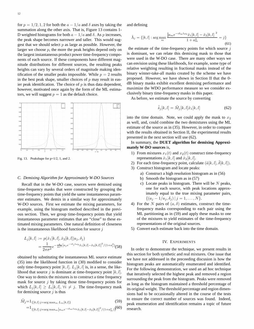
In order to evaluate the usefulness of the histogram as a pa-rameter estimator, a smoothed histogram was created for eachof the tests used to generate Figure 8 and the peak locationof the histogram was used as the symmetric attenuation anddelay estimate. Figure 12 contains the results of these tests.Each estimator histogram consisted of 401-by-401 points witha delay range from -6 to 6 samples and symmetric attenua-tion from -1.2 to 1.2, and the smoothing kernel had parameters(B, D) = (.12, .2). Comparing Figure 8 and Figure 12, weconclude that the histogram based estimators are superior to thepreviously considered ML motivated estimators.

−5 −4 −3 −2 −1 0 1 2 3 4 5−5

−4

−3

−2

−1

0

1

2

3

4

5

actual δ

estim

ate

d δ

p=1/2p=1 p=2

(a)

−1 −0.8 −0.6 −0.4 −0.2 0 0.2 0.4 0.6 0.8 1−1

−0.8

−0.6

−0.4

−0.2

0

0.2

0.4

0.6

0.8

1

actual a−1/a

estim

ate

d a

−1

/a

p=1/2p=1 p=2

(b)

Fig. 12. Histogram Delay and Attenuation Estimator Comparison. Plot (a)compares estimated δ versus true δ for the smoothed histogram peak estimatorswith p = 1/2, 1, 2 for δ ranging linearly from -5 to 5 samples as a − 1/aranges linearly 0.15 to -0.15. Plot (b) compares estimated a − 1/a to the truea − 1/a. Both plots were generated using a model of 5 source mixing.

The similar estimator performance for different choices of pin Figure 12 suggests that the choice of p should be driven byother concerns. Identifying the peaks in the histogram is thecrucial step in the separation process. Two important criteriafor the weighting exponent p selection are (1) the shape aroundthe peak (the “peak shape”) and (2) the relative peak heights.In order to aid in peak identification, we want the peak shapeto be narrow and tall, and we want the peaks to be roughly ofthe same height. Figure 13 compares the histogram peak shapes

12

for p = 1/2, 1, 2 for both the a − 1/a and δ axes by taking thesummation along the other axis. That is, Figure 13 contains 1-D weighted histograms for both a− 1/a and δ. As p increases,the peak shape becomes narrower and taller. This would sug-gest that we should select p as large as possible. However, thelarger we choose p, the more the peak heights depend only onthe largest instantaneous product power time-frequency compo-nents of each source. If these components have different mag-nitude distributions for different sources, the resulting peaksheights can vary by several orders of magnitude making iden-tification of the smaller peaks impossible. While p = 2 resultsin the best peak shape, smaller choices of p may result in eas-ier peak identification. The choice of p is thus data dependent,however, motivated once again by the form of the ML estima-tors, we will suggest p = 1 as the default choice.

−2 −1.5 −1 −0.5 0 0.5 1 1.5 20

0.01

0.02

0.03

0.04

0.05

0.06

0.07

0.08

0.09

0.1

δ

p=1/2p=1 p=2

−1 −0.8 −0.6 −0.4 −0.2 0 0.2 0.4 0.6 0.8 10

0.01

0.02

0.03

0.04

0.05

0.06

0.07

0.08

0.09

a − 1/a

p=1/2p=1 p=2

Fig. 13. Peakshape for p=1/2, 1, and 2.

C. Demixing Algorithm for Approximately W-DO Sources

Recall that in the W-DO case, sources were demixed usingtime-frequency masks that were constructed by grouping thetime-frequency points that yield the same instantaneous param-eter estimates. We demix in a similar way for approximatelyW-DO sources. First we estimate the mixing parameters, forexample, using the histogram method described in the previ-ous section. Then, we group time-frequency points that yieldinstantaneous parameter estimates that are “close” to these es-timated mixing parameters. One natural definition of closenessis the instantaneous likelihood function for source j

Lj [k, l] := p(x1[k, l], x2[k, l]|aj , δj)

=1

2πσ2e−

12σ2 |aje−iδj lω0 x1[k,l]−x2[k,l]|2/(1+a2

j )(58)

obtained by substituting the instantaneous ML source estimate(35) into the likelihood function in (30) modified to consideronly time-frequency point [k, l]. Lj [k, l] is, in a sense, the like-lihood that source j is dominant at time-frequency point [k, l].One way to demix the mixtures is to construct a time frequencymask for source j by taking those time-frequency points forwhich Lj [k, l] ≥ Li[k, l], ∀i 6= j. The time-frequency maskfor demixing source j is thus

Mj=1[k,l]:j=arg maxm Lm[k,l] (59)

=1[k,l]:j=arg maxm|ame−iδmlω0 x1[k,l]−x2[k,l]|2/(1+a2

m)(60)

and defining

Λj = [k, l] : arg maxm

ame−iδmlω0 x1[k, l] − x2[k, l] 2

1 + a2m

= j

(61)the estimate of the time-frequency points for which source j

is dominant, we can relate this demixing mask to those thatwere used in the W-DO case. There are many other ways wecan envision using these likelihoods, for example, some type ofrelative weighting resulting in fractional masks instead of thebinary winner-take-all masks created by the scheme we haveproposed. However, we have shown in Section II that the 0-dB binary masks exhibit excellent demixing performance andmaximize the WDO performance measure so we consider ex-clusively binary time-frequency masks in this paper.

As before, we estimate the source by converting

˜sj [k, l] = Mj [k, l]x1[k, l] (62)

into the time domain. Note, we could apply the mask to x2

as well, and, could combine the two demixtures using the MLestimate of the source as in (35). However, in order to comparewith the results obtained in Section II, the experimental resultspresented in the next section will use (62).

In summary, the DUET algorithm for demixing Approxi-mately W-DO sources is,

1) From mixtures x1(t) and x2(t) construct time-frequencyrepresentations x1[k, l] and x2[k, l].

2) For each time-frequency point, calculate (a[k, l], δ[k, l]).3) Construct histogram and locate peaks:

a) Construct a high resolution histogram as in (56)b) Smooth the histogram as in (57)c) Locate peaks in histogram. There will be N peaks,

one for each source, with peak locations approx-imately equal to the true mixing parameter pairs,(aj − 1/aj , δj) | j = 1, . . . , N.

4) For the N pairs of (a, δ) estimates, construct the time-frequency masks corresponding to each pair using theML partitioning as in (59) and apply these masks to oneof the mixtures to yield estimates of the time-frequencyrepresentations of the original sources.

5) Convert each estimate back into the time domain.

IV. EXPERIMENTS

In order to demonstrate the technique, we present results inthis section for both synthetic and real mixtures. One issue thatwe have not addressed in the preceeding discusion is how thehistogram peaks are automatically enumerated and identified.For the following demonstration, we used an ad hoc techniquethat iteratively selected the highest peak and removed a regionsurrounding the peak from the histogram. Peaks were removedas long as the histogram maintained a threshold percentage ofits original weight. The threshold percentage and region dimen-sions had to be occasionally altered in the course of the teststo ensure the correct number of sources was found. Indeed,peak enumeration and identification remains a topic of futureresearch.

13

A. Synthetic mixtures

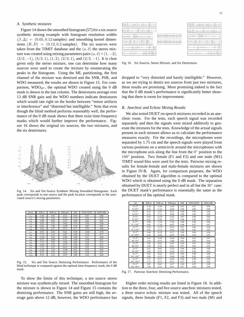
Figure 14 shows the smoothed histogram (57) for a six sourcesynthetic mixing example with histogram resolution widths(β, ∆) = (0.05, 0.12 samples) and smoothing kernel dimen-sions (B, D) = (0.12, 0.2 samples). The six sources weretaken from the TIMIT database and the (a, δ) the stereo mix-ture was created using mixing parameters pairs (a, δ) = (1,−2),(3/2,−1), (3/2, 1), (1, 2), (2/3, 1), and (2/3,−1). It is cleargiven only the stereo mixture, one can determine how manysources were used to create the mixture by enumerating thepeaks in the histogram. Using the ML partitioning, the firstchannel of the mixture was demixed and the SNR, PSR, andWDO measured; the results are shown in Figure 15. For com-parison, WDOΦ0 , the optimal WDO created using the 0 dBmask is shown in the last column. The demixtures average over13 dB SNR gain and the WDO numbers indicate demixtureswhich would rate right on the border between “minor artifactsor interference” and “distorted but intelligible.” Note that eventhough the blind method performs reasonably well, the perfor-mance of the 0 dB mask shows that there exist time-frequencymasks which would further improve the performance. Fig-ure 16 shows the original six sources, the two mixtures, andthe six demixtures.

−2−1

01

2

−1

−0.5

0

0.5

1

0.5

1

1.5

2

2.5

3

δa − 1/a

−2−1

01

2

−1

−0.5

0

0.5

1

0.2

0.4

0.6

0.8

1

1.2

1.4

1.6

1.8

δa − 1/a

Fig. 14. Six and Ten Source Synthetic Mixing Smoothed Histograms. Eachpeak corresponds to one source and the peak location corresponds to the asso-ciated source’s mixing parameters.

source SNR in SNR out SNR gain PSR WDO DUET WDO 0dB

s1 -7.29 5.92 13.21 0.76 0.57 0.80s2 -7.29 5.24 12.53 0.78 0.55 0.78s3 -5.08 6.60 11.67 0.80 0.62 0.81s4 -9.29 5.35 14.63 0.79 0.56 0.69s5 -5.03 7.06 12.09 0.78 0.63 0.81s6 -9.28 5.47 14.75 0.77 0.55 0.66

s1 -9.74 -0.32 9.42 0.58 -0.04 0.70s2 -7.73 3.14 10.87 0.66 0.34 0.77s3 -11.64 3.43 15.06 0.68 0.37 0.64s4 -9.72 -0.60 9.13 0.58 -0.09 0.67s5 -7.73 3.93 11.66 0.66 0.39 0.73s6 -11.61 3.14 14.75 0.56 0.29 0.51s7 -7.75 2.57 10.31 0.56 0.25 0.74s8 -11.62 1.36 12.98 0.61 0.16 0.62s9 -9.72 4.70 14.42 0.60 0.39 0.67

s10 -9.74 3.33 13.07 0.60 0.32 0.64

Fig. 15. Six and Ten Source Demixing Performance. Performance of theblind technique is compared against the optimal time-frequency mask, the 0 dBmask.

To show the limits of this technique, a ten source stereomixture was synthetically mixed. The smoothed histogram forthe mixture is shown in Figure 14 and Figure 15 contains thedemixing performance. The SNR gains are still high, the av-erage gain above 12 dB, however, the WDO performance has

Fig. 16. Six Sources, Stereo Mixture, and Six Demixtures.

dropped to “very distorted and barely intelligible.” However,as we are trying to demix ten sources from just two mixtures,these results are promising. More promising indeed is the factthat the 0 dB mask’s performance is significantly better show-ing that there is room for improvement.

B. Anechoic and Echoic Mixing Results

We also tested DUET on speech mixtures recorded in an ane-choic room. For the tests, each speech signal was recordedseparately and then the signals were mixed additively to gen-erate the mixtures for the tests. Knowledge of the actual signalspresent in each mixture allows us to calculate the performancemeasures exactly. For the recordings, the microphones wereseparated by 1.75 cm and the speech signals were played fromvarious positions on a semicircle around the microphones withthe microphone axis along the line from the 0 position to the180 position. Two female (F1 and F2) and one male (M1)TIMIT sound files were used for the tests. Pairwise mixing re-sults for female-female and male-female mixtures are shownin Figure IV-B. Again, for comparison purposes, the WDOobtained by the DUET algorithm is compared to the optimalWDO which is obtained using the 0 dB mask. The separationobtained by DUET is nearly perfect and in all but the 30 case:the DUET mask’s performance is essentially the same as theperformance of the optimal mask.

test SNR in SNR out SNR gain PSR WDO DUET WDO 0dB

F1 0 -0.58 12.69 13.26 0.92 0.87 0.96F2 30 0.58 11.25 10.68 0.96 0.89 0.96F1 0 -0.54 15.97 16.51 0.98 0.95 0.96

F2 60 0.54 17.21 16.68 0.98 0.96 0.96F1 0 -0.62 15.29 15.91 0.97 0.94 0.94

F2 90 0.62 15.69 15.07 0.98 0.95 0.95F1 0 -0.49 17.50 17.99 0.98 0.96 0.96

F2 120 0.49 17.36 16.87 0.98 0.97 0.97F1 0 -0.50 15.79 16.29 0.97 0.94 0.94

F2 150 0.50 15.51 15.01 0.98 0.95 0.95F1 0 -0.44 16.29 16.73 0.96 0.94 0.94

F2 180 0.44 14.49 14.05 0.98 0.94 0.95

F1 0 3.54 13.99 10.46 0.96 0.92 0.97M1 30 -3.54 10.35 13.88 0.91 0.83 0.94

F1 0 3.60 18.42 14.81 0.99 0.97 0.98M1 60 -3.60 15.41 19.01 0.97 0.94 0.95

F1 0 3.63 18.92 15.29 0.99 0.98 0.98M1 90 -3.63 15.91 19.54 0.97 0.95 0.95

F1 0 3.69 19.91 16.22 0.99 0.98 0.98M1 120 -3.69 15.79 19.48 0.98 0.95 0.95

F1 0 3.75 19.57 15.82 0.99 0.98 0.98M1 150 -3.75 16.37 20.12 0.97 0.95 0.95

F1 0 3.90 18.47 14.57 0.99 0.97 0.98M1 180 -3.90 15.51 19.41 0.97 0.94 0.94

Fig. 17. Pairwise Anechoic Demixing Performance.

Higher order mixing results are listed in Figure 18. In addi-tion to the three, four, and five source anechoic mixtures tested,a three source echoic mixture was tested. All of the speechsignals, three female (F1, F2, and F3) and two male (M1 and

14

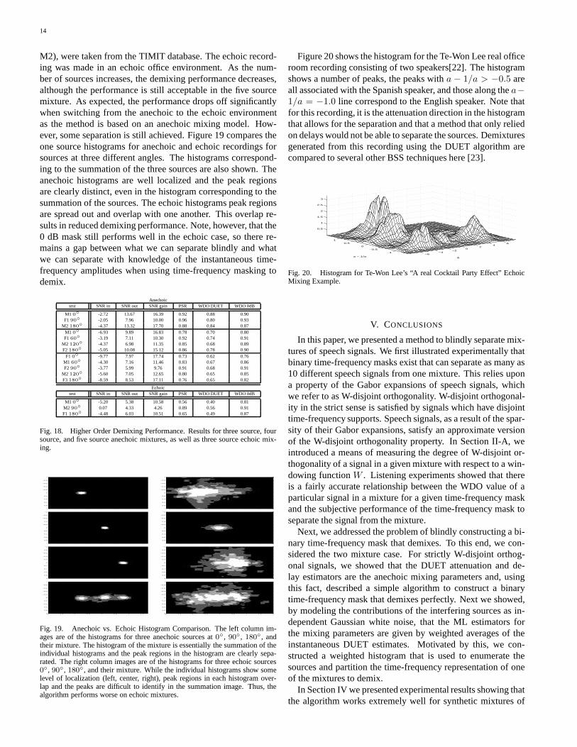
M2), were taken from the TIMIT database. The echoic record-ing was made in an echoic office environment. As the num-ber of sources increases, the demixing performance decreases,although the performance is still acceptable in the five sourcemixture. As expected, the performance drops off significantlywhen switching from the anechoic to the echoic environmentas the method is based on an anechoic mixing model. How-ever, some separation is still achieved. Figure 19 compares theone source histograms for anechoic and echoic recordings forsources at three different angles. The histograms correspond-ing to the summation of the three sources are also shown. Theanechoic histograms are well localized and the peak regionsare clearly distinct, even in the histogram corresponding to thesummation of the sources. The echoic histograms peak regionsare spread out and overlap with one another. This overlap re-sults in reduced demixing performance. Note, however, that the0 dB mask still performs well in the echoic case, so there re-mains a gap between what we can separate blindly and whatwe can separate with knowledge of the instantaneous time-frequency amplitudes when using time-frequency masking todemix.

Anechoictest SNR in SNR out SNR gain PSR WDO DUET WDO 0dB

M1 0 -2.72 13.67 16.39 0.92 0.88 0.90F1 90 -2.05 7.96 10.00 0.96 0.80 0.93

M2 180 -4.37 13.32 17.70 0.88 0.84 0.87M1 0 -6.93 9.89 16.83 0.78 0.70 0.80F1 60 -3.19 7.11 10.30 0.92 0.74 0.91

M2 120 -4.37 6.98 11.35 0.85 0.68 0.89F2 180 -5.05 10.08 15.12 0.86 0.78 0.90

F1 0 -9.77 7.97 17.74 0.73 0.62 0.76M1 60 -4.30 7.16 11.46 0.83 0.67 0.86F2 90 -3.77 5.99 9.76 0.91 0.68 0.91

M2 120 -5.60 7.05 12.65 0.80 0.65 0.85F3 180 -8.59 8.53 17.11 0.76 0.65 0.82

Echoictest SNR in SNR out SNR gain PSR WDO DUET WDO 0dB

M1 0 -5.20 5.38 10.58 0.56 0.40 0.81M2 90 0.07 4.33 4.26 0.89 0.56 0.91F1 180 -4.48 6.03 10.51 0.65 0.49 0.87

Fig. 18. Higher Order Demixing Performance. Results for three source, foursource, and five source anechoic mixtures, as well as three source echoic mix-ing.

−2 −1.5 −1 −0.5 0 0.5 1 1.5 2

−1

−0.8

−0.6

−0.4

−0.2

0

0.2

0.4

0.6

0.8

1−2 −1.5 −1 −0.5 0 0.5 1 1.5 2

−1

−0.8

−0.6

−0.4

−0.2

0

0.2

0.4

0.6

0.8

1

−2 −1.5 −1 −0.5 0 0.5 1 1.5 2

−1

−0.8

−0.6

−0.4

−0.2

0

0.2

0.4

0.6

0.8

1−2 −1.5 −1 −0.5 0 0.5 1 1.5 2

−1

−0.8

−0.6

−0.4

−0.2

0

0.2

0.4

0.6

0.8

1

−2 −1.5 −1 −0.5 0 0.5 1 1.5 2

−1

−0.8

−0.6

−0.4

−0.2

0

0.2

0.4

0.6

0.8

1−2 −1.5 −1 −0.5 0 0.5 1 1.5 2

−1

−0.8

−0.6

−0.4

−0.2

0

0.2

0.4

0.6

0.8

1

−2 −1.5 −1 −0.5 0 0.5 1 1.5 2

−1

−0.8

−0.6

−0.4

−0.2

0

0.2

0.4

0.6

0.8

1−2 −1.5 −1 −0.5 0 0.5 1 1.5 2

−1

−0.8

−0.6

−0.4

−0.2

0

0.2

0.4

0.6

0.8

1

Fig. 19. Anechoic vs. Echoic Histogram Comparison. The left column im-ages are of the histograms for three anechoic sources at 0, 90, 180, andtheir mixture. The histogram of the mixture is essentially the summation of theindividual histograms and the peak regions in the histogram are clearly sepa-rated. The right column images are of the histograms for three echoic sources0, 90, 180, and their mixture. While the individual histograms show somelevel of localization (left, center, right), peak regions in each histogram over-lap and the peaks are difficult to identify in the summation image. Thus, thealgorithm performs worse on echoic mixtures.

Figure 20 shows the histogram for the Te-Won Lee real officeroom recording consisting of two speakers[22]. The histogramshows a number of peaks, the peaks with a − 1/a > −0.5 areall associated with the Spanish speaker, and those along the a−1/a = −1.0 line correspond to the English speaker. Note thatfor this recording, it is the attenuation direction in the histogramthat allows for the separation and that a method that only reliedon delays would not be able to separate the sources. Demixturesgenerated from this recording using the DUET algorithm arecompared to several other BSS techniques here [23].

−6−4

−20

24

6

−1

−0.5

0

0.5

1

0.5

1

1.5

2

2.5

3

δa − 1/a

Fig. 20. Histogram for Te-Won Lee’s “A real Cocktail Party Effect” EchoicMixing Example.

V. CONCLUSIONS

In this paper, we presented a method to blindly separate mix-tures of speech signals. We first illustrated experimentally thatbinary time-frequency masks exist that can separate as many as10 different speech signals from one mixture. This relies upona property of the Gabor expansions of speech signals, whichwe refer to as W-disjoint orthogonality. W-disjoint orthogonal-ity in the strict sense is satisfied by signals which have disjointtime-frequency supports. Speech signals, as a result of the spar-sity of their Gabor expansions, satisfy an approximate versionof the W-disjoint orthogonality property. In Section II-A, weintroduced a means of measuring the degree of W-disjoint or-thogonality of a signal in a given mixture with respect to a win-dowing function W . Listening experiments showed that thereis a fairly accurate relationship between the WDO value of aparticular signal in a mixture for a given time-frequency maskand the subjective performance of the time-frequency mask toseparate the signal from the mixture.

Next, we addressed the problem of blindly constructing a bi-nary time-frequency mask that demixes. To this end, we con-sidered the two mixture case. For strictly W-disjoint orthog-onal signals, we showed that the DUET attenuation and de-lay estimators are the anechoic mixing parameters and, usingthis fact, described a simple algorithm to construct a binarytime-frequency mask that demixes perfectly. Next we showed,by modeling the contributions of the interfering sources as in-dependent Gaussian white noise, that the ML estimators forthe mixing parameters are given by weighted averages of theinstantaneous DUET estimates. Motivated by this, we con-structed a weighted histogram that is used to enumerate thesources and partition the time-frequency representation of oneof the mixtures to demix.

In Section IV we presented experimental results showing thatthe algorithm works extremely well for synthetic mixtures of

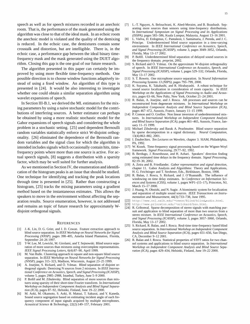
15

speech as well as for speech mixtures recorded in an anechoicroom. That is, the performance of the mask generated using thealgorithm was close to that of the ideal mask. In an echoic roomthe anechoic model is violated and the quality of the demixingis reduced. In the echoic case, the demixtures contain somecrosstalk and distortion, but are intelligible. There is, in theechoic case, a performance gap between the ideal binary time-frequency mask and the mask generated using the DUET algo-rithm. Closing this gap is the one goal of our future research.

The algorithm presented in this paper can certainly be im-proved by using more flexible time-frequency methods. Onepossible direction is to choose window functions adaptively in-stead of using a fixed window. An algorithm of this type ispresented in [24]. It would be also interesting to investigatewhether one could obtain a similar separation algorithm usingwavelet expansions of speech.

In Section III-B.1, we derived the ML estimators for the mix-ing parameters by using a naive stochastic model for the contri-butions of interfering sources. A better estimator can perhapsbe obtained by using a more realistic stochastic model for theGabor expansions of speech signals and considering the wholeproblem in a stochastic setting. [25] used dependent Bernoullirandom variables statistically enforce strict W-disjoint orthog-onality. [26] eliminated the dependence of the Bernoulli ran-dom variables and the signal class for which the algorithm isintended includes signals which occasionally contain hits, time-frequency points where more than one source is active. For ac-tual speech signals, [8] suggests a distribution with a sparsityfactor, which may be well suited for further analysis.

As we mentioned in Section IV, the enumeration and identifi-cation of the histogram peaks is an issue that should be studied.One technique for identifying and tracking the peak locationsthrough time is presented in [25]. Rather than constructing ahistogram, [25] tracks the mixing parameters using a gradientmethod based on the instantaneous estimates. This allows thespeakers to move in the environment without affecting the sep-aration results. Source enumeration, however, is not addressedand remains an topic of future research for approximately W-disjoint orthogonal signals.

REFERENCES

[1] J.-K. Lin, D. G. Grier, and J. D. Cowan. Feature extraction approach toblind source separation. In IEEE Workshop on Neural Networks for SignalProcessing (NNSP), pages 398–405, Amelia Island Plantation, Florida,September 24–26 1997.

[2] T-W. Lee, M. Lewicki, M. Girolami, and T. Sejnowski. Blind source sepa-ration of more sources than mixtures using overcomplete representations.IEEE Signal Processing Letters, 6(4):87–90, April 1999.

[3] M. Van Hulle. Clustering approach to square and non-square blind sourceseparation. In IEEE Workshop on Neural Networks for Signal Processing(NNSP), pages 315–323, Madison, Wisconsin, August 23–25 1999.

[4] A. Jourjine, S. Rickard, and O. Yılmaz. Blind separation of disjoint or-thogonal signals: Demixing N sources from 2 mixtures. In IEEE Interna-tional Conference on Acoustics, Speech, and Signal Processing (ICASSP),volume 5, pages 2985–2988, Istanbul, Turkey, June 5–9 2000.

[5] P. Bofill and M. Zibulevsky. Blind separation of more sources than mix-tures using sparsity of their short-time Fourier transform. In InternationalWorkshop on Independent Component Analysis and Blind Signal Separa-tion (ICA), pages 87–92, Helsinki, Finland, June 19–22 2000.

[6] M. Aoki, M. Okamoto, S. Aoki, H. Matsui, T. Sakurai, and Y. Kaneda.Sound source segregation based on estimating incident angle of each fre-quency component of input signals acquired by multiple microphones.Acoustical Science & Technology, 22(2):149–157, February 2001.

[7] L.-T. Nguyen, A. Belouchrani, K. Abed-Meraim, and B. Boashash. Sep-arating more sources than sensors using time-frequency distributions.In International Symposium on Signal Processing and its Applications(ISSPA), pages 583–586, Kuala Lumpur, Malaysia, August 13–16 2001.

[8] L. Vielva, D. Erdogmus, C. Pantaleon, I. Santamaria, J. Pereda, and J. C.Principe. Underdetermined blind source separation in a time-varyingenvironment. In IEEE International Conference on Acoustics, Speech,and Signal Processing (ICASSP), volume 3, pages 3049–3052, Orlando,Florida, May 13–17 2002.

[9] P. Bofill. Underdetermined blind separation of delayed sound sources inthe frequency domain. preprint, 2002.

[10] S. Rickard and O. Yılmaz. On the approximate W-disjoint orthogonalityof speech. In IEEE International Conference on Acoustics, Speech, andSignal Processing (ICASSP), volume 1, pages 529–532, Orlando, Florida,May 13–17 2002.

[11] S. T. Roweis. One microphone source separation. In Neural InformationProcessing Systems 13 (NIPS), pages 793–799, 2000.

[12] K. Suyama, K. Takahashi, and R. Hirabayashi. A robust technique forsound source localization in consideration of room capacity. In IEEEWorkshop on the Applications of Signal Processing to Audio and Acous-tics, pages 63–66, New Paltz, New York, October 21–24 2001.

[13] R. Balan, A. Jourjine, and J. Rosca. AR processes and sources can bereconstructed from degenerate mixtures. In International Workshop onIndependent Component Analysis and Blind Source Separation (ICA),pages 467–472, Aussois, France, January 11–15 1999.

[14] P. Comon and O. Grellier. Non linear inversion of underdetermined mix-tures. In International Workshop on Independent Component Analysisand Blind Source Separation (ICA), pages 461–465, Aussois, France, Jan-uary 11–15 1999.

[15] Michael Zibulevsky and Barak A. Pearlmutter. Blind source separationby sparse decomposition in a signal dictionary. Neural Computation,13(4):863–882, 2001.

[16] I. Daubechies. Ten Lectures on Wavelets, chapter 3. SIAM, Philadelphia,PA, 1992.

[17] W. Kozek. Time-frequency signal processing based on the Wigner-Weylframework. Signal Processing, 29:77–92, 1992.

[18] B. Berdugo, J. Rosenhouse, and H. Azhari. Speakers’ direction findingusing estimated time delays in the frequency domain. Signal Processing,82:19–30, 2002.

[19] A. Zeira and B. Friedlander. Gabor representation and signal detection,chapter 11. Gabor Analysis and Algorithms: Theory and Applications,H. G. Feichtinger and T. Strohmer, Eds., Birkhauser, Boston, 1998.

[20] R. Balan, J. Rosca, S. Rickard, and J. O’Ruanaidh. The influence ofwindowing on time delay estimates. In Conference on Information Sci-ences and Systems (CISS), volume 1, pages WP1–(15–17), Princeton, NJ,March 15–17 2000.

[21] J. Huang, N. Ohnishi, and N. Sugie. A biomimetic system for localizationand separation of multiple sound sources. IEEE Transactions on Instru-mentation and Measurement, 44(3):733–738, June 1995.

[22] http://www.cnl.salk.edu/∼tewon/Blind/blind audio.html.[23] http://www.princeton.edu/∼srickard/bss.html.[24] R. Gribonval. Sparse decomposition of stereo signals with matching pur-

suit and application to blind separation of more than two sources from astereo mixture. In IEEE International Conference on Acoustics, Speech,and Signal Processing (ICASSP), volume 3, pages 3057–3060, Orlando,Florida, May 13–17 2002.

[25] S. Rickard, R. Balan, and J. Rosca. Real-time time-frequency based blindsource separation. In International Workshop on Independent ComponentAnalysis and Blind Source Separation (ICA), pages 651–656, San Diego,CA, December 9–12 2001.

[26] R. Balan and J. Rosca. Statistical properties of STFT ratios for two chan-nel systems and applications to blind source separation. In InternationalWorkshop on Independent Component Analysis and Blind Source Sepa-ration (ICA), pages 429–434, Helsinki, Finland, June 19–22 2000.