shape analysis of concurrent programs - bgufrankel/verification2008/moolysagivshape-bgu.pdf ·...

Shape Analysis of Concurrent Programs

Mooly Sagiv

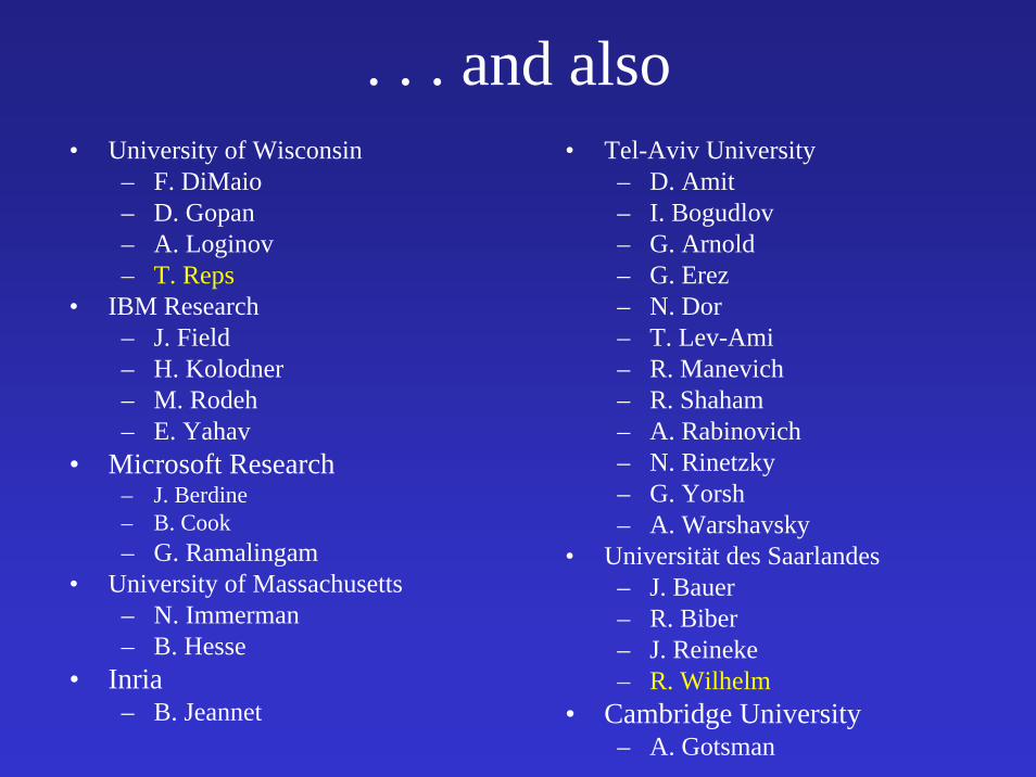
• Tel-Aviv University– D. Amit– I. Bogudlov– G. Arnold– G. Erez– N. Dor– T. Lev-Ami– R. Manevich– R. Shaham– A. Rabinovich– N. Rinetzky– G. Yorsh– A. Warshavsky

• Universität des Saarlandes– J. Bauer– R. Biber– J. Reineke– R. Wilhelm

• Cambridge University– A. Gotsman

. . . and also• University of Wisconsin

– F. DiMaio– D. Gopan– A. Loginov– T. Reps

• IBM Research– J. Field– H. Kolodner– M. Rodeh– E. Yahav

• Microsoft Research– J. Berdine– B. Cook– G. Ramalingam

• University of Massachusetts– N. Immerman– B. Hesse

• Inria– B. Jeannet

Shape Analysis [Jones and Muchnick 1981]

• Determine the possible shapes of a dynamically allocated data structureat a given program point

• Motivation– More efficient compilation

• Compile-time garbage collection• Parallelization

– Verification

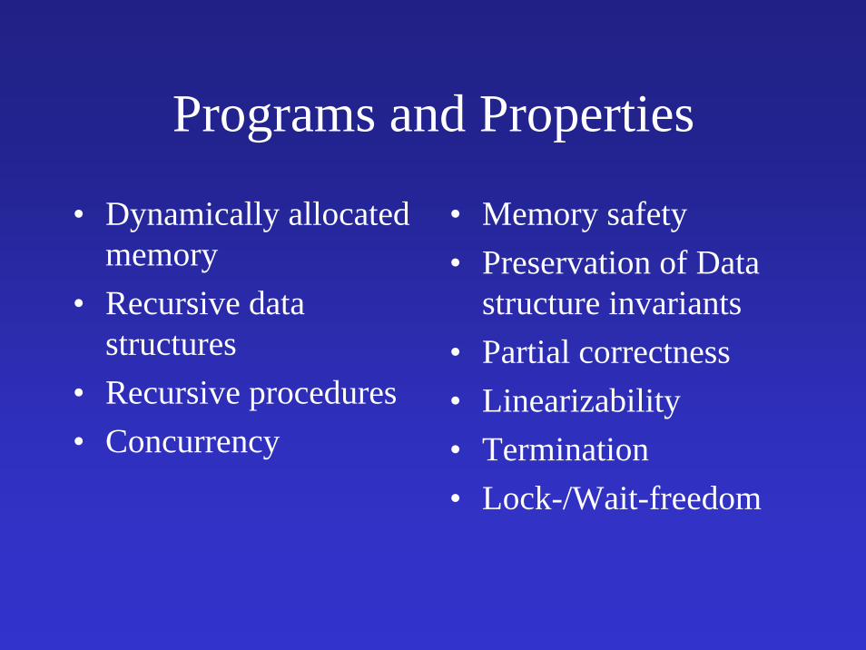
Programs and Properties

• Dynamically allocated memory

• Recursive data structures

• Recursive procedures• Concurrency

• Memory safety • Preservation of Data

structure invariants• Partial correctness• Linearizability• Termination• Lock-/Wait-freedom

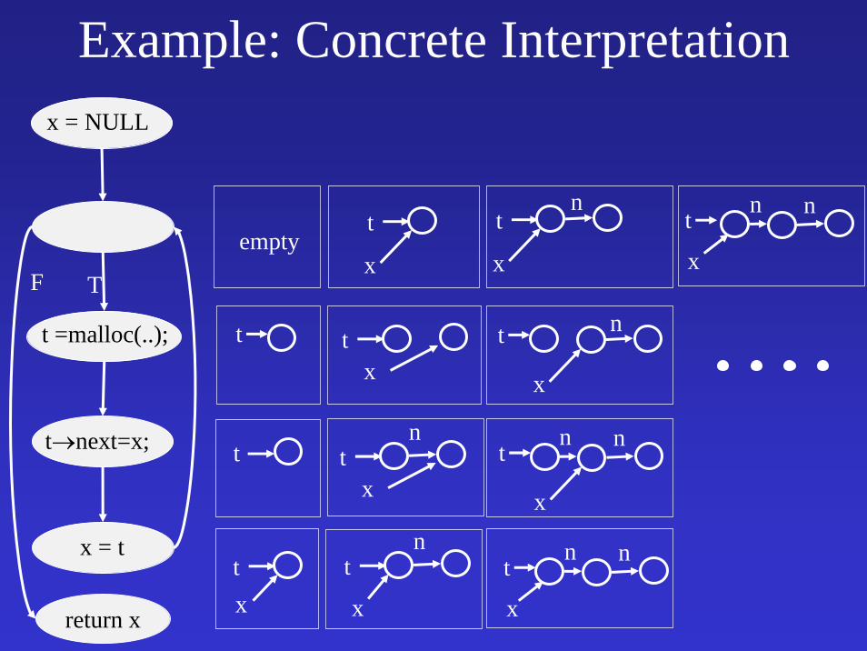
Example: Concrete Interpretation

x

t n nt

x

n

x

t n

x

tn n

x

tn n

xtt

x

ntt

nt

x

tx

t

xempty

return x

x = t

t =malloc(..);

t→next=x;

x = NULL

TF

Shape Analysis

t

x

n

x

t n

x

tn n

xtt

x

ntt

nt

x

tx

t

xempty

x

tn

n

x

tn

n

n

x

tn

t n

xn

x

tn

nreturn x

x = t

t =malloc(..);

t→next=x;

x = NULL

TF

Outline

• Abstract interpretation in the nutshell• Shape Analysis• Handling concurrent programs

Abstract Interpretation[Cousot & Cousot]

• Checking interesting program properties is undecidable

• Use abstractions• Every verified property holds (sound)• But may fail to prove properties which

always hold (incomplete)– false alarms

• Minimal false alarms

Simplified Abstract Interpretation

Concrete domain(unbounded)

Abstract domain(bounded)

βββ

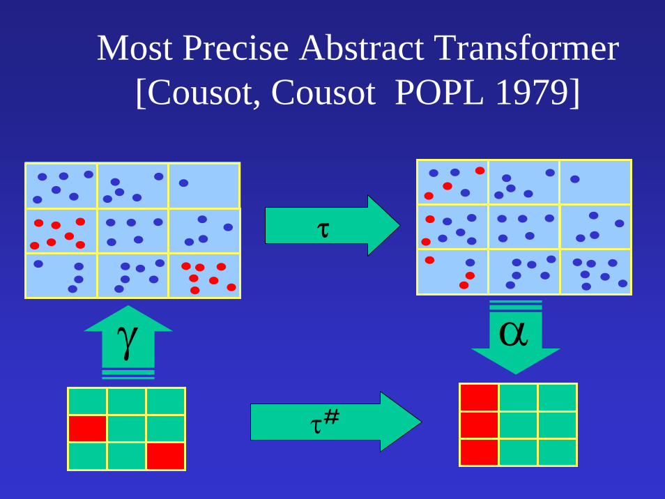
Most Precise Abstract Transformer[Cousot, Cousot POPL 1979]

γ α

τ#

τ

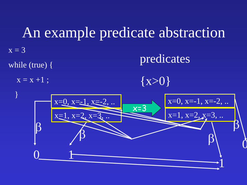
An example predicate abstraction

predicates

{x>0}

x = 3

while (true) {

x = x +1 ;

}x=0, x=-1, x=-2, ..

x=1, x=2, x=3, ..

1

β

0

β

x=0, x=-1, x=-2, ..

x=1, x=2, x=3, ..x=3

1

β 0β


predicates

{x>0}

x = 3

while (true) {

x = x +1 ;

}x=0, x=-1, x=-2, ..

x=1, x=2, x=3, ..

1

β

0

β

x=0, x=-1, x=-2, ..

x=1, x=2, x=3, ..x=x+1

1

β 0β


predicates

{x>0}

x = 3

while (true) {

x = x +1 ;

}

{0, 1}

{1}{1}

{1} {1}

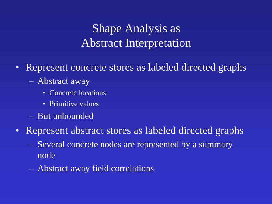
Shape Analysis as Abstract Interpretation

• Represent concrete stores as labeled directed graphs– Abstract away

• Concrete locations• Primitive values

– But unbounded

• Represent abstract stores as labeled directed graphs– Several concrete nodes are represented by a summary

node– Abstract away field correlations

Representing Concrete Stores by Logical Structures

• Parametric vocabulary• Heap

– Locations ≈ Individuals– Program variables ≈ Unary relations– Fields ≈ Binary relations

Representing Concrete Storesby Logical Structures

– U = {u1, u2, u3, u4, u5}– x = {u1}, p = {u3}– n = {<u1, u2>, <u2, u3>, <u3, u4>, <u4, u5>}– rx = {u1, u2, u3, u4, u5}– rp = {u3, u4, u5}

u1 u2 u3 u4 u5xn n n n

p

rx rx rx rx rx

rp rp rp

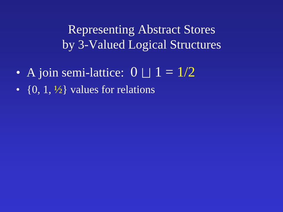
Representing Abstract Stores by 3-Valued Logical Structures

• A join semi-lattice: 0 7 1 = 1/2• {0, 1, ½} values for relations

Canonical Abstraction (β)• Partition the individuals into equivalence classes based on the

values of their unary relations– Every individual is mapped into its equivalence class

• Collapse binary relations via 7

– pS (u’1, u’2) = 7 {pB (u1, u2) | f(u1)=u’1, f(u2)=u’2) }

• At most 2A abstract individuals

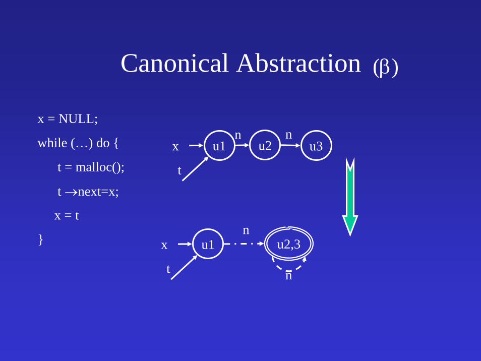
Canonical Abstraction

x = NULL;

while (…) do {

t = malloc();

t →next=x;

x = t

}

u1x

t

u2 u3n n

u1x

t

u2,3n

n

(β)


rxx rxrx rp

n n n

p

rx rp

rp

nn

rx rx rxrp rx rp rx rpxn n

rp

n n

p

rxn

Canonical Abstraction w/o reachability

u1 u2 u4 u5 u6xn n

p

n n

a1 a2 a3n n

p

u3n

n

x

n

Canonical Abstractions as Formulas[Yorsh’03, Kuncak’04, Wies’07 ]

rx

x

rx rx, rpn n n

p

rx, rp

rp

nn

∀v: (x(v) ∧rx(v)∧¬p(v)∧¬rp(v)) ∨(¬x(v) ∧rx(v)∧¬p(x)∧¬rp(v)) ∨(¬x(v) ∧rx(v)∧p(v)∧rp(v)) ∨

(¬x(v) ∧rx(v)∧¬p(v)∧rp(v)))

∀v:rx(v) ⇔ ∃w: x(w) ∧ n*(w, v)∀v:rp(v) ⇔ ∃w: p(w) ∧ n*(w, v)

Canonical Abstractions as Formulas[Yorsh’03, Kuncak’04, Wies’07 ]

∀v, w: (¬x(v) ∧rx(v)∧¬p(v)∧rp(v)) ∧ (x(w) ∧rx(w)∧¬p(w)∧¬rp(w))

⇒

¬n(v, w)

rx

x

rx rx, rpn n n

p

rx, rp

rp

nn ¬n


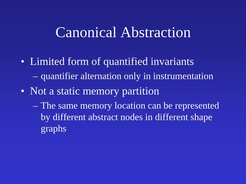
• Limited form of quantified invariants∨i

∀v: ∨j {ϕi, j(v) } ∧∀v, w: ∧m, n {ϕi,m (v) ∧ ϕi, n (w)⇒ εi, m, n (v, w)} – quantifier alternation and transitive closure only

in instrumentation– Bounded number of distinctions

Most Precise Abstract Transformer[Cousot, Cousot POPL 1979]

γ α

τ#

τ

yx

yx

yx

yx ...

xy

yx

...

xy

Best Transformer (x = x → n)

γ

Concrete Semantics

canonical abstraction

yx

xy

Non-Fixed-Partition

x = x→n

yx

y

x


• Limited form of quantified invariants– quantifier alternation only in instrumentation

• Not a static memory partition– The same memory location can be represented

by different abstract nodes in different shape graphs

Shape Analysis

t

x

n

x

t n

x

tn n

xtt

x

ntt

nt

x

tx

t

xempty

x

tn

n

x

tn

n

n

x

tn

t n

xn

x

tn

nreturn x

x = t

t =malloc(..);

t→next=x;

x = NULL

TF

[TOPLAS’02, Lev-Ami, SAS’00]

• Concrete transformers using first order formulas• Effective algorithms for computing transformers

– Partial concretization– 3-valued logic Kleene evaluation– Finite differencing & incremental algorithms

[Reps, ESOP’03]

• A parametric yacc like system[TVLA]– http://www.cs.tau.ac.il/~tvla

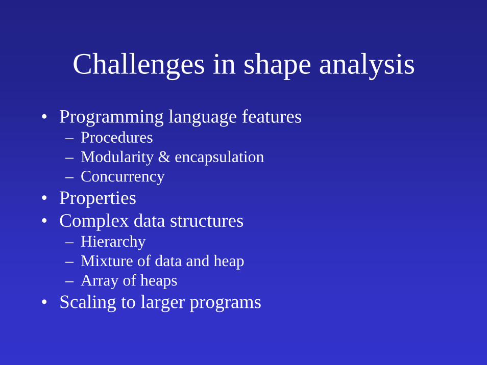
Challenges in shape analysis

• Programming language features– Procedures– Modularity & encapsulation– Concurrency

• Properties• Complex data structures

– Hierarchy– Mixture of data and heap– Array of heaps

• Scaling to larger programs

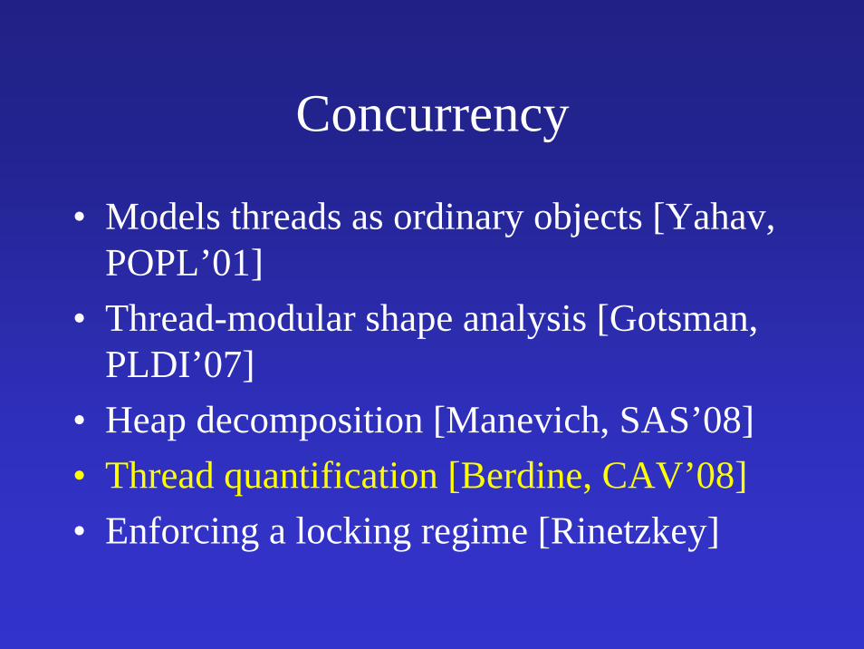
Concurrency

• Models threads as ordinary objects [Yahav, POPL’01]

• Thread-modular shape analysis [Gotsman, PLDI’07]

• Heap decomposition [Manevich, SAS’08]• Thread quantification [Berdine, CAV’08]• Enforcing a locking regime [Rinetzkey]

Thread Quantification for Concurrent Shape Analysis

J. Berdine, T. Lev-Ami, R. Manevich, G. Ramalingam, and M. Sagiv

CAV’08

Non-blocking stack [Treiber 1986][1] void push(Stack *S, data_type v) {[2] Node *x = alloc(sizeof(Node));[3] x->d = v;[4] do {[5] Node *t = S->Top;[6] x->n = t;[7] } while (!CAS(&S->Top,t,x));[8] }

[9] data_type pop(Stack *S){[10] do {[11] Node *t = S->Top;[12] if (t == NULL)[13] return EMPTY;[14] Node *s = t->n;[15] data_type r = s->d;[16] } while (!CAS(&S->Top,t,s));[17] return r;[18] }

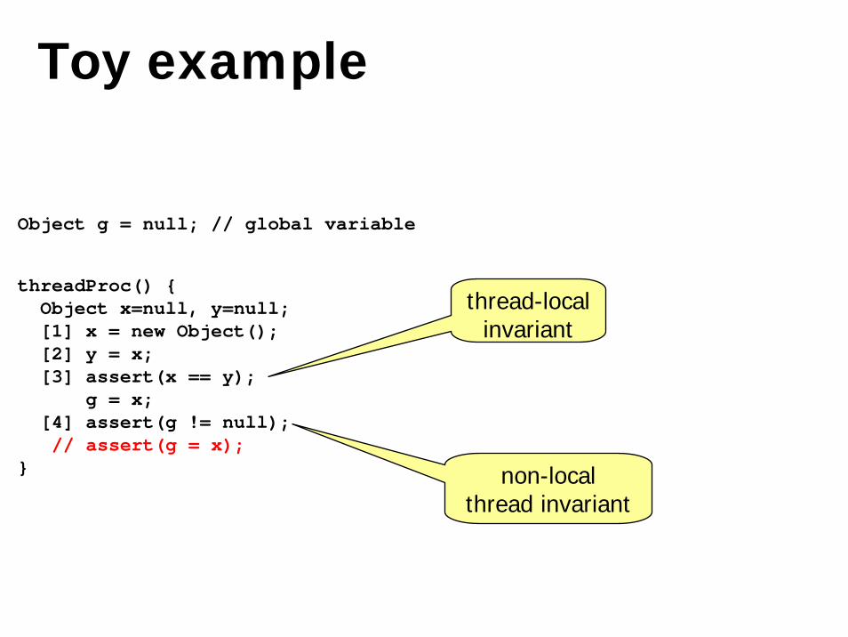
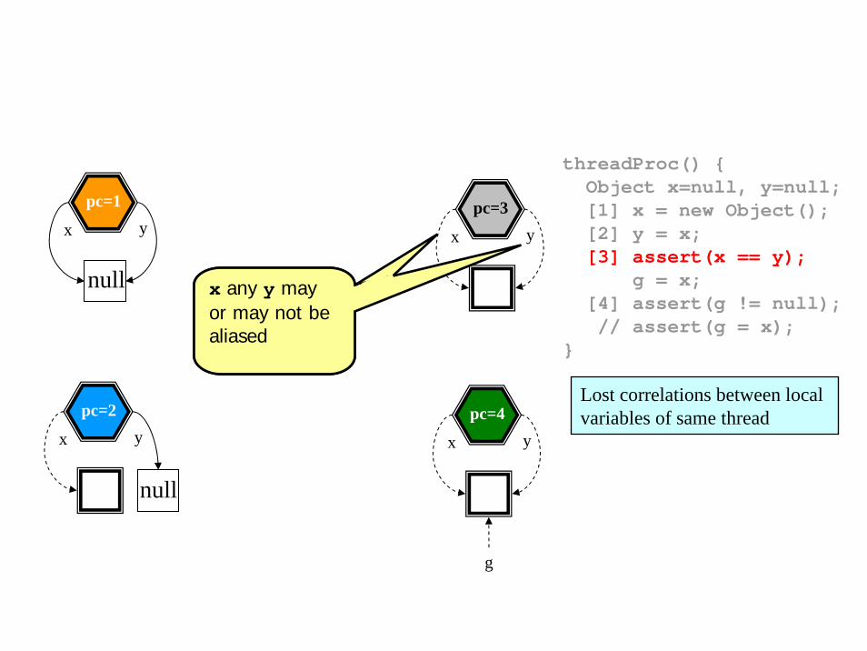
Toy example

threadProc() {Object x=null, y=null;[1] x = new Object();[2] y = x;[3] assert(x == y);

g = x;[4] assert(g != null);// assert(g = x);

}

thread-local invariant

non-localthread invariant

Object g = null; // global variable

Toy example (one thread)



}

Object g = null; // global variable x ypc=1

null

gx ypc=2

null

gx ypc=3

null

gx ypc=4

null

g




}

x ypc=1

null

g

x ypc=3

null

g

x ypc=2

null

g

x ypc=4

null

g



pc = 1 . x = y = g = null

- pc = 2 . x ≠ null . y = g = null

- pc = 3 . x = y ≠ null . g = null

- pc = 4 . x = y = g . g ≠ null

What about an unbounded number of threads?




}

Multiple threads

x ypc=1

x ypc=2

null

null

…x ypc=1

null

x ypc=2

null

…

x ypc=3

x ypc=3

…

x ypc=4

g

x ypc=4

…x ypc=4

Collapse threads at the same locationYahav, POPL’01

x ypc=1

x ypc=2

null

null

…x ypc=1

null

x ypc=2

null

…

x ypc=3

x ypc=3

…

x ypc=4

g

x ypc=4

…x ypc=4

x ypc=1

x ypc=2

null

null

x ypc=3

x ypc=4

g



}

Lost correlations between local variables of same thread

Executed by many threadsx any y may or may not be aliased

Quantified Abstraction

pc(t) = 1 .…

- pc(t) = 2 .…

- pc(t) = 3 . x(t) = y(t) …

- pc(t) = 4 . x(t) = y(t) . g≠null

- pc(t) = 4 . x(t) = y(t) = g . g≠null…

∀tthreadProc() {Object x=null, y=null;[1] x = new Object();[2] y = x;[3] assert(x == y);


}

Object g = null; // global variableEach disjunct represents an abstractionof state from the perspective of one thread

Lost information: number of threads Indexed predicate

Intuition for quantified abstraction

x ypc=1

x ypc=2

null

null

…x ypc=1

null

x ypc=2

null

…

x ypc=3

x ypc=3

…

x ypc=4

g

x ypc=4

…x ypc=4

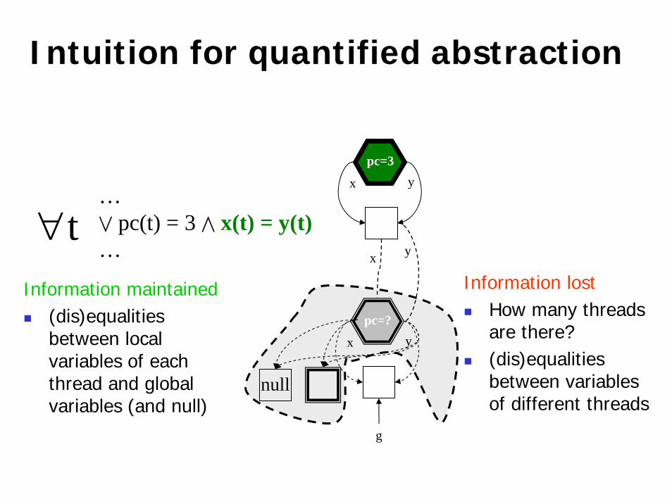
Intuition for quantified abstraction

x ypc=3

x ypc=?

g

null

…- pc(t) = 3 . x(t) = y(t)…

∀tyx

Information maintained(dis)equalitiesbetween local variables of each thread and global variables (and null)

Information lostHow many threads are there?(dis)equalitiesbetween variables of different threads

Properties of quantified abstraction

Abstracts the number of threads(Similar to counter abstraction with ≥0)

Thread-modular abstractionEach disjunction focuses on a single thread

Coarse abstraction of “environment”Captures correlations between values of local

variables of a thread and the global stateAbstracts away correlations between the values local variables of different threads

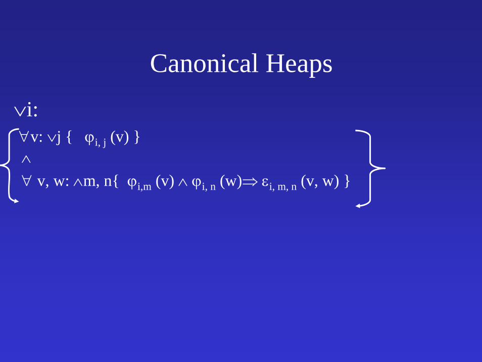
∨i: ∀v: ∨j { ϕi, j (v) } ∧

∀ v, w: ∧m, n{ ϕi,m (v) ∧ ϕi, n (w)⇒ εi, m, n (v, w) }

Canonical Heaps

∀t: ∨i: ∀v: ∨j {ϕi, j (t, v)}

∧ ∀ v, w: ∧m, n{ ϕi,m (t, v) ∧ ϕi, n (t, w)⇒ εi, m, n (t, v, w) }

“Lifted” Canonical Heaps

Missing

•Heuristics for computing transformers–Quantifier instantiation

•Proving linearizability–[Amit, CAV’07]–Fixed linearization point–Bounded concrete differences between sequential and

concurrent implementarions–Simplified memory model

•Garbage collection•Sequential consistency

Non-blocking stack [Treiber 1986][1] void push(Stack *S, data_type v) {[2] Node *x = alloc(sizeof(Node));[3] x->d = v;[4] do {[5] Node *t = S->Top;[6] x->n = t;[7] } while (!CAS(&S->Top,t,x));[8] }

[9] data_type pop(Stack *S){[10] do {[11] Node *t = S->Top;[12] if (t == NULL)[13] return EMPTY;[14] Node *s = t->n;[15] data_type r = s->d;[16] } while (!CAS(&S->Top,t,s));[17] return r;[18] }

Verified Programs #states time (sec.)

Treiber’s stack[1986]

764 7

Two-lock queue[Doherty and Groves FORTE’04]

3,415

10,333

17

Non-blocking queue[Michael and Scott PODC’96]

252

Experimental results

First automatic verification of linearizabilityfor unbounded number of threads

Summary

• Shape analysis is an interesting abstract interpretation problem

• Limited forms of quantified invariants can be utilized to prove interesting properties

• Scaling shape analysis to realistic programs is still an open problem

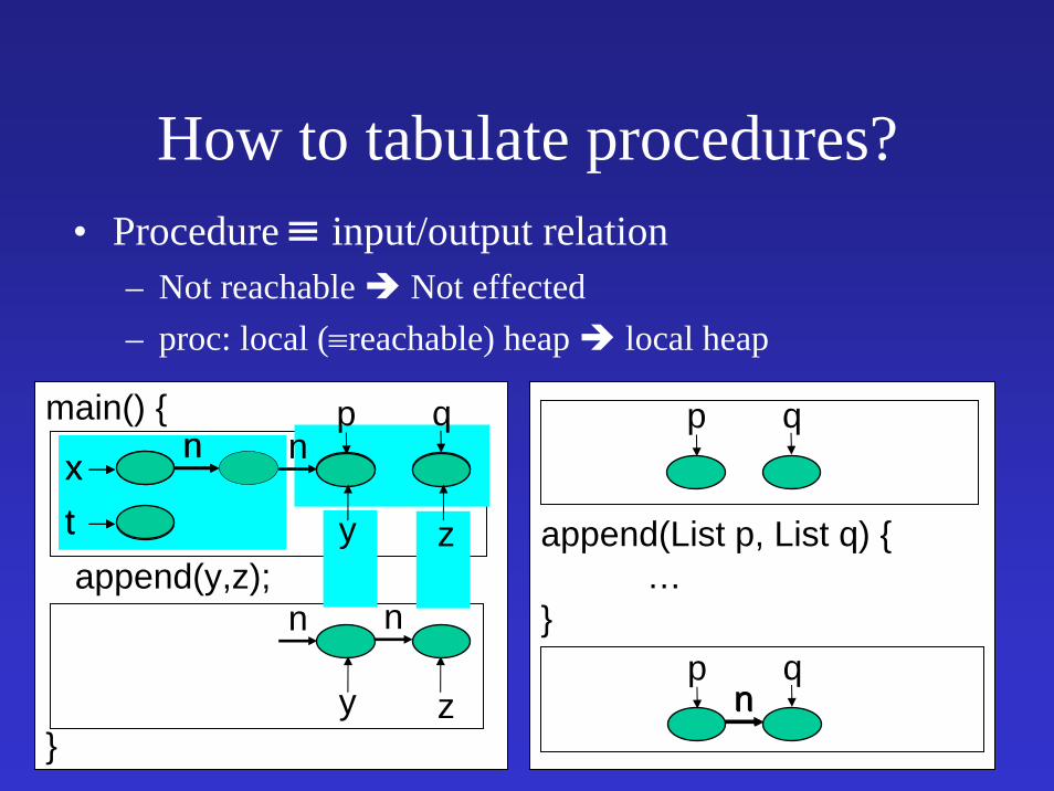
main() {

append(y,z);

}

• Procedure ≡ input/output relation– Not reachable Not effected– proc: local (≡reachable) heap local heap

How to tabulate procedures?

append(List p, List q) {…

}

nx n

t

y

n

z

n

p q p q

n

y z

p qn

x n

t

main() {

append(y,z);

}

y nn

z

n

How to handle sharing?• External sharing may break the functional view

append(List p, List q) {…

}

nn

t z

x n

p qnn

p qnn

ty

p qnn n

x

append(y,z);

What’s the difference?

nn

t z

y

x

1st Example 2nd Example

append(y,z);

nx n

t y z

Cutpoints

• An object is a cutpoint for an invocation– Reachable from actual parameters– Not pointed to by an actual parameter– Reachable without going through a parameter

append(y,z) append(y,z)

y

x

nn

t z

y nn

t zn n

Introducing local heap semanticsOperational semantics

Abstract transformer

Local heap Operational semantics

~γ’ α’

Interprocedural shape analysis• Procedure ≡ input/output relation

p qn

nrqrp rp

qpn

nrp rq

n rp

q qrqrq

qprp

qprp rq

n rprq

Input Output

… rp

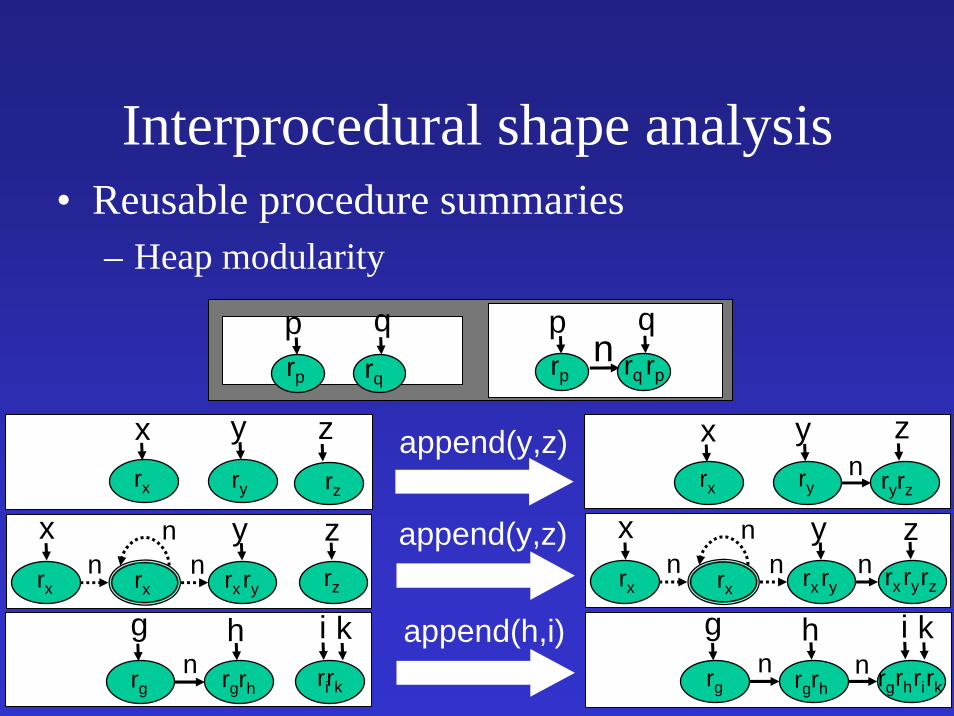
Interprocedural shape analysis• Reusable procedure summaries

– Heap modularity

qprp rq

n rp

qprp rq

g h i kn n

g h i kn rgrgrg rgrh rh rirkrhrgrirk

append(h,i)

yx zn

nn n rxryrz

yx zn

nn rz rx ryrxrxrx ryrx rx

append(y,z)

yn

zxappend(y,z)y zxrx ry rz ryrx ryrz

Handling Larger Programs• Staged analysis • Specialized abstractions

– Counterexample guided refinement• Coercer abstractions

– Weaker summary nodes [Arnold, SAS’06]– Special join operator [Manevich, SAS’04, TACAS’07, Yang’08] – Heterogeneous abstractions [Yahav, PLDI’04]

• Implementation techniques– Optimizing transformers [Bogodlov, CAV’07]– Optimizing GC– Reducing static size– Partial evaluation– Persistent data structures [Manevich, SAS’04]– …

shape analysis of concurrent programs - bgufrankel/verification2008/moolysagivshape-bgu.pdf ·...

Documents