machine learning for the quantified self - wordpress.com · machine learning for the quantified...
TRANSCRIPT
Machine Learning for the Quantified Self
Lecture 1 Introduction

Quantified Self definition (1)
• Term first coined by Gary Wolf and Kevin Kelly in Wired Magazine
• Let’s watch a video first: https://www.youtube.com/watch?v=OrAo8oBBFIo
2
Quantified Self definition (2)
• What is the quantified self? – Swan (2013): “The quantified self is any
individual engaged in the self-tracking of any kind of biological, physical, behavioral, or environmental information. There is a proactive stance toward obtaining information and acting on it.”
3
Quantified Self definition (3)
– We: “The quantified self is any individual engaged in the self-tracking of any kind of biological, physical, behavioral, or environmental information. The self-tracking is driven by a certain goal of the individual with a desire to act upon the collected information.”
4
Quantified Self: measurements
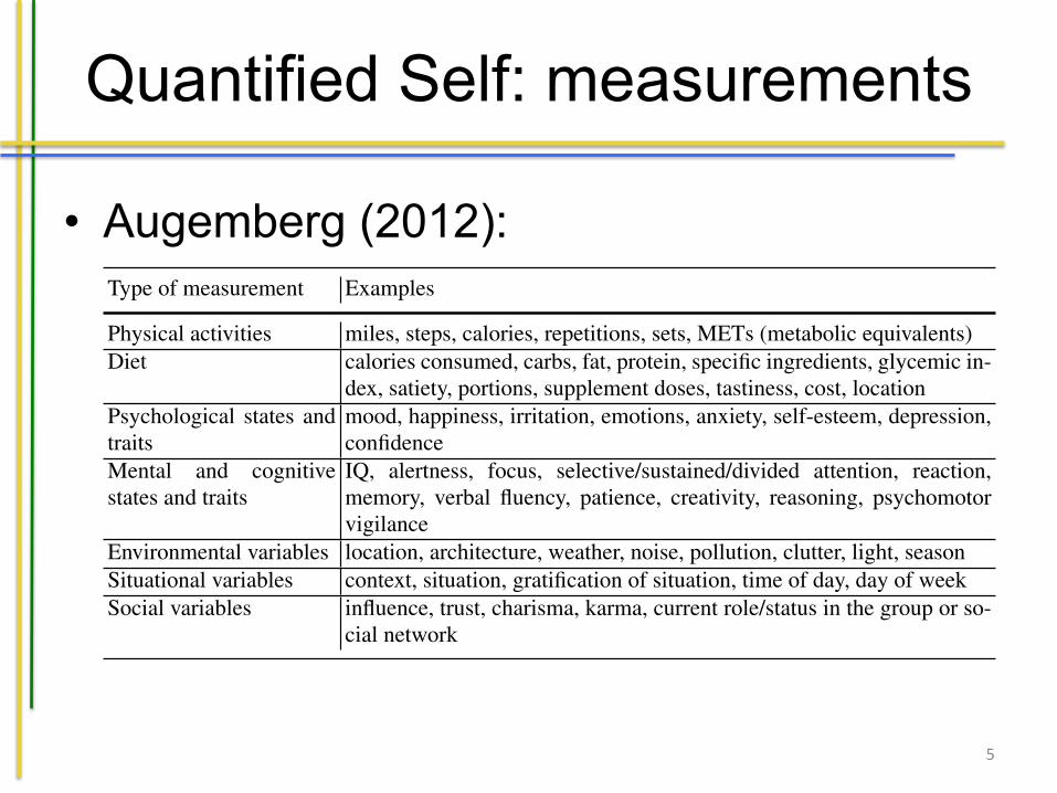
• Augemberg (2012):
5
1.2 The goal of this book 3
Table 1.1: Examples of quantified self data (cf. Augemberg [8], taken fromSwan [102])
Type of measurement Examples
Physical activities miles, steps, calories, repetitions, sets, METs (metabolic equivalents)Diet calories consumed, carbs, fat, protein, specific ingredients, glycemic in-
dex, satiety, portions, supplement doses, tastiness, cost, locationPsychological states andtraits
mood, happiness, irritation, emotions, anxiety, self-esteem, depression,confidence
Mental and cognitivestates and traits
IQ, alertness, focus, selective/sustained/divided attention, reaction,memory, verbal fluency, patience, creativity, reasoning, psychomotorvigilance
Environmental variables location, architecture, weather, noise, pollution, clutter, light, seasonSituational variables context, situation, gratification of situation, time of day, day of weekSocial variables influence, trust, charisma, karma, current role/status in the group or so-
cial network
aspects of the quantified self), self-design (control and optimize yourself using thedata), self-association (enjoying being part of a community and to relate yourselfto the community), and self-entertainment (enjoying the entertainment value of theself-tracking) as important motivational factors for quantified selfs. They refer tothese factors as ”Five-Factor-Framework of Self-Tracking Motivations”.
1.2 The goal of this book
Not that we know what the quantified self is, what do we aim to achieve with thisbook? As you might have noticed, the quantified self can and will most likely resultin a huge amount of data being collected about individuals. An immediate questionthat pops up is how to make sense of this data. Even enthusiasts such as Arnold willnot be able to oversee it all, and might miss valuable information. This is wheremachine learning comes into play. Many definitions of machine learning exist. Inour case, we define machine learning as follows:
Definition 1.3. Machine learning is to automatically identify patterns from data.
This book aims to show how machine learning can be applied to quantified self data:to let the computer automatically extract patterns from collected data and facilitatea user to act upon insights effectively, thus contributing to the goal of the user. Letus make this a bit more concrete by means of some examples using our two fellowsArnold and Bruce:
• Advising the training to make most progress towards a certain goal based on pastoutcomes of training.
Quantified Self: why? (1)
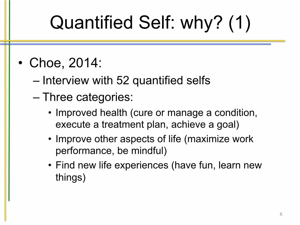
• Choe, 2014: – Interview with 52 quantified selfs – Three categories:
• Improved health (cure or manage a condition, execute a treatment plan, achieve a goal)
• Improve other aspects of life (maximize work performance, be mindful)
• Find new life experiences (have fun, learn new things)
6

Quantified Self: why? (2)
• Gimpel, 2013: – Identify “Five-Factor Framework of Self-
Tracking Motivations: • Self-healing (become healthy) • Self-discipline (rewarding aspects of it) • Self-design (control and optimize “yourself”) • Self-association (associated with movement) • Self-entertainment (entertainment value)
7
Quantified Self: Arnold and Bruce
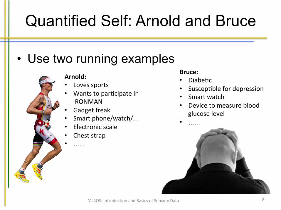
• Use two running examples
8
Arnold:• Lovessports• Wantstopar4cipatein
IRONMAN• Gadgetfreak• Smartphone/watch/…• Electronicscale• Cheststrap• ……
Bruce:• Diabe4c• Suscep4blefordepression• Smartwatch• Devicetomeasureblood
glucoselevel• ……
ML4QS:Introduc4onandBasicsofSensoryData
Moving on the machine learning
• Machine learning: “Machine learning is to automatically identify patterns from data”
• What could we learn for Arnold and Bruce?
9
What could we learn?
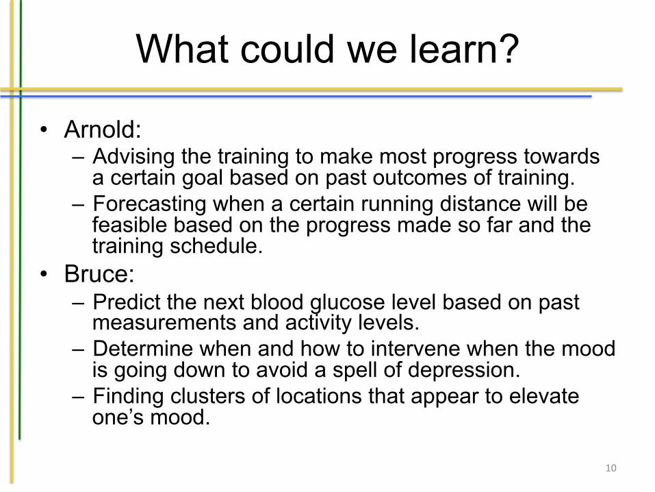
• Arnold: – Advising the training to make most progress towards
a certain goal based on past outcomes of training. – Forecasting when a certain running distance will be
feasible based on the progress made so far and the training schedule.
• Bruce: – Predict the next blood glucose level based on past
measurements and activity levels. – Determine when and how to intervene when the mood
is going down to avoid a spell of depression. – Finding clusters of locations that appear to elevate
one’s mood.
10
Why is the Quantified Self so different?
• Sensory noise • Missing measurements • Temporal data • Interaction with a user • Learn over multiple datasets
11
Basic Terminology (1)
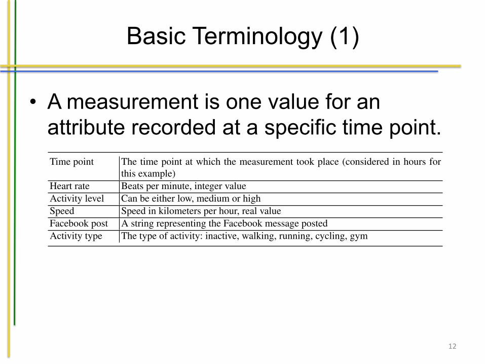
• A measurement is one value for an attribute recorded at a specific time point.
12
1.3 Basic terminology 5
Table 1.2: Attributes in example dataset
Time point The time point at which the measurement took place (considered in hours forthis example)
Heart rate Beats per minute, integer valueActivity level Can be either low, medium or highSpeed Speed in kilometers per hour, real valueFacebook post A string representing the Facebook message postedActivity type The type of activity: inactive, walking, running, cycling, gym
Measurements can have values of different data types: they can be numerical, orcategorical with an ordering (ordinal) or without (nominal). Let us consider an ex-ample dataset associated with Arnold. The attributes are shown in Table 1.2. Thetime point is not considered to be part of the attributes (though listed for the sakeof completeness) as it is an inherent part of the measurement itself. For the othervariables, the speed and heart rate would be considered a numerical measurement.The Facebook posts and activity type are both nominal attributes and the activitylevel is ordinal.
Measurements frequently come in sequences, for instance a sequence of valuesfor a heart rate. This is what we call a time series:
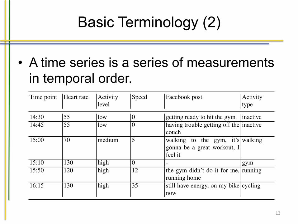
Definition 1.5. A time series is a series of measurements in temporal order.
Time series often form the basis to interpret measurements. To exemplify the notionof a time series, an example of data collected for each of the attributes discussed inTable 1.2 is shown in Table 1.3. In the table, the columns represent the attributeswhile the rows are the measurements performed at the indicated time points. Here,one can consider the sequence [55, 55, 70, 130, 120, 130] as an example of a timeseries for the attribute heart rate.
Table 1.3: Example dataset
Time point Heart rate Activitylevel
Speed Facebook post Activitytype
14:30 55 low 0 getting ready to hit the gym inactive14:45 55 low 0 having trouble getting off the
couchinactive
15:00 70 medium 5 walking to the gym, it’sgonna be a great workout, Ifeel it
walking
15:10 130 high 0 - gym15:50 120 high 12 the gym didn’t do it for me,
running homerunning
16:15 130 high 35 still have energy, on my bikenow
cycling
Basic Terminology (2)
• A time series is a series of measurements in temporal order.
13
1.3 Basic terminology 5
Table 1.2: Attributes in example dataset
Time point The time point at which the measurement took place (considered in hours forthis example)
Heart rate Beats per minute, integer valueActivity level Can be either low, medium or highSpeed Speed in kilometers per hour, real valueFacebook post A string representing the Facebook message postedActivity type The type of activity: inactive, walking, running, cycling, gym
Measurements can have values of different data types: they can be numerical, orcategorical with an ordering (ordinal) or without (nominal). Let us consider an ex-ample dataset associated with Arnold. The attributes are shown in Table 1.2. Thetime point is not considered to be part of the attributes (though listed for the sakeof completeness) as it is an inherent part of the measurement itself. For the othervariables, the speed and heart rate would be considered a numerical measurement.The Facebook posts and activity type are both nominal attributes and the activitylevel is ordinal.
Measurements frequently come in sequences, for instance a sequence of valuesfor a heart rate. This is what we call a time series:
Definition 1.5. A time series is a series of measurements in temporal order.
Time series often form the basis to interpret measurements. To exemplify the notionof a time series, an example of data collected for each of the attributes discussed inTable 1.2 is shown in Table 1.3. In the table, the columns represent the attributeswhile the rows are the measurements performed at the indicated time points. Here,one can consider the sequence [55, 55, 70, 130, 120, 130] as an example of a timeseries for the attribute heart rate.
Table 1.3: Example dataset
Time point Heart rate Activitylevel
Speed Facebook post Activitytype
14:30 55 low 0 getting ready to hit the gym inactive14:45 55 low 0 having trouble getting off the
couchinactive
15:00 70 medium 5 walking to the gym, it’sgonna be a great workout, Ifeel it
walking
15:10 130 high 0 - gym15:50 120 high 12 the gym didn’t do it for me,
running homerunning
16:15 130 high 35 still have energy, on my bikenow
cycling
Basic Terminology (3)
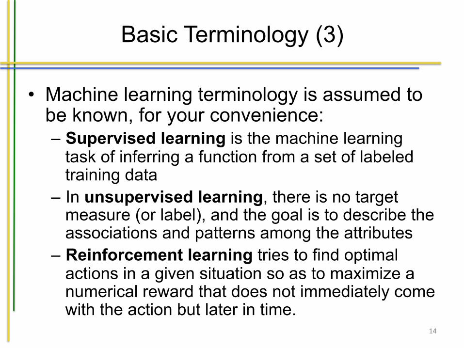
• Machine learning terminology is assumed to be known, for your convenience: – Supervised learning is the machine learning
task of inferring a function from a set of labeled training data
– In unsupervised learning, there is no target measure (or label), and the goal is to describe the associations and patterns among the attributes
– Reinforcement learning tries to find optimal actions in a given situation so as to maximize a numerical reward that does not immediately come with the action but later in time.
14
Mathematical notation (1)
15
8 1 Introduction
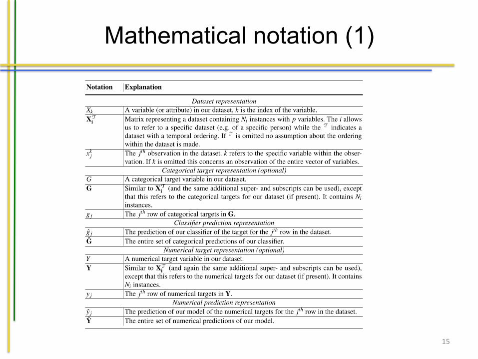
Table 1.4: Formal notation
Notation Explanation
Dataset representationXk A variable (or attribute) in our dataset, k is the index of the variable.XT
i Matrix representing a dataset containing Ni instances with p variables. The i allowsus to refer to a specific dataset (e.g. of a specific person) while the T indicates adataset with a temporal ordering. If T is omitted no assumption about the orderingwithin the dataset is made.
xkj The jth observation in the dataset. k refers to the specific variable within the obser-
vation. If k is omitted this concerns an observation of the entire vector of variables.Categorical target representation (optional)
G A categorical target variable in our dataset.G Similar to XT
i (and the same additional super- and subscripts can be used), exceptthat this refers to the categorical targets for our dataset (if present). It contains Niinstances.
g j The jth row of categorical targets in G.Classifier prediction representation
g j The prediction of our classifier of the target for the jth row in the dataset.G The entire set of categorical predictions of our classifier.
Numerical target representation (optional)Y A numerical target variable in our dataset.Y Similar to XT
i (and again the same additional super- and subscripts can be used),except that this refers to the numerical targets for our dataset (if present). It containsNi instances.
y j The jth row of numerical targets in Y.Numerical prediction representation
y j The prediction of our model of the numerical targets for the jth row in the dataset.Y The entire set of numerical predictions of our model.
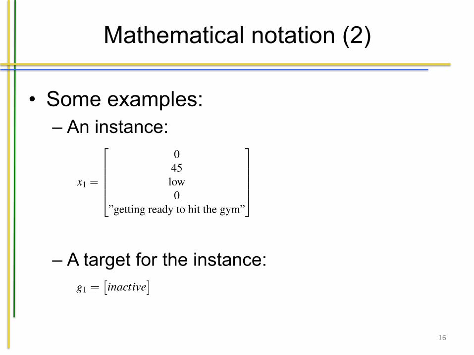
vector of observations of our p variables where j identifies the instance. j can takethe values j = 1, . . . ,N with N being the number of observations. For example:
x1 =
2
66664
045low0
”getting ready to hit the gym”
3
77775
If we want to refer to a specific value of one variable within the instance we will usethe notation xk
j where j refers to the instance and k = 1, . . . , p (p is the number ofvariables) to the position of the variable in the vector (e.g. x2
1 = 45). Here, depend-ing on the nature of the instances, j could also represent the notion of time as theinstances might form a sequence of measurements over time, i.e. j = tstart , . . . , tendassuming a discrete time scale. Given that we have p elements in our vector, wecan represent an entire dataset as a matrix (similar to the table notation we have
Mathematical notation (2)
16
• Some examples: – An instance:
– A target for the instance:
8 1 Introduction
Table 1.4: Formal notation
Notation Explanation
Dataset representationXk A variable (or attribute) in our dataset, k is the index of the variable.XT
i Matrix representing a dataset containing Ni instances with p variables. The i allowsus to refer to a specific dataset (e.g. of a specific person) while the T indicates adataset with a temporal ordering. If T is omitted no assumption about the orderingwithin the dataset is made.
xkj The jth observation in the dataset. k refers to the specific variable within the obser-
vation. If k is omitted this concerns an observation of the entire vector of variables.Categorical target representation (optional)
G A categorical target variable in our dataset.G Similar to XT
i (and the same additional super- and subscripts can be used), exceptthat this refers to the categorical targets for our dataset (if present). It contains Niinstances.
g j The jth row of categorical targets in G.Classifier prediction representation
g j The prediction of our classifier of the target for the jth row in the dataset.G The entire set of categorical predictions of our classifier.
Numerical target representation (optional)Y A numerical target variable in our dataset.Y Similar to XT
i (and again the same additional super- and subscripts can be used),except that this refers to the numerical targets for our dataset (if present). It containsNi instances.
y j The jth row of numerical targets in Y.Numerical prediction representation
y j The prediction of our model of the numerical targets for the jth row in the dataset.Y The entire set of numerical predictions of our model.
vector of observations of our p variables where j identifies the instance. j can takethe values j = 1, . . . ,N with N being the number of observations. For example:
x1 =
2
66664
045low0
”getting ready to hit the gym”
3
77775
If we want to refer to a specific value of one variable within the instance we will usethe notation xk
j where j refers to the instance and k = 1, . . . , p (p is the number ofvariables) to the position of the variable in the vector (e.g. x2
1 = 45). Here, depend-ing on the nature of the instances, j could also represent the notion of time as theinstances might form a sequence of measurements over time, i.e. j = tstart , . . . , tendassuming a discrete time scale. Given that we have p elements in our vector, wecan represent an entire dataset as a matrix (similar to the table notation we have
1.5 Overview of the book 9
seen before). This will result in an N ⇥ p matrix. As x j is defined to be a columnvector (our example x1 was as well) each row j is the transposed version of x j, i.e.xT
j . This matrix will be noted in boldface with X. Sometimes we use an index toidentify a specific dataset (e.g. the dataset originating from Arnold or Bruce), wenote this as Xi. If the instances represent a sequence of measurements over time wewill use XT to denote a time series training set (this will be an important distinctionfor later Chapters). If we omit the T we make no assumption about the ordering.The same conventions as we have just introduced are used for the outputs for thecase of supervised learning. The entire set of targets for all instances are specifiedby Y and G for numerical and categorical targets respectively. We have very dis-tinct cases for numerical and categorical cases as the learning algorithms for bothcases typically work very differently. The predicted output of our supervised modelover all instances will be denoted as Y or G. Individual targets and predictions forthe instance i are expressed as yi and gi for the target values and yi and gi for thepredictions. Our target output for our input vector x1 would be:
g1 =⇥inactive
⇤
Hence, we end up with a training dataset of the form (x j,y j) or (x j,g j) where j =1, . . . ,N. An overview of the notation is presented in Table 1.4.
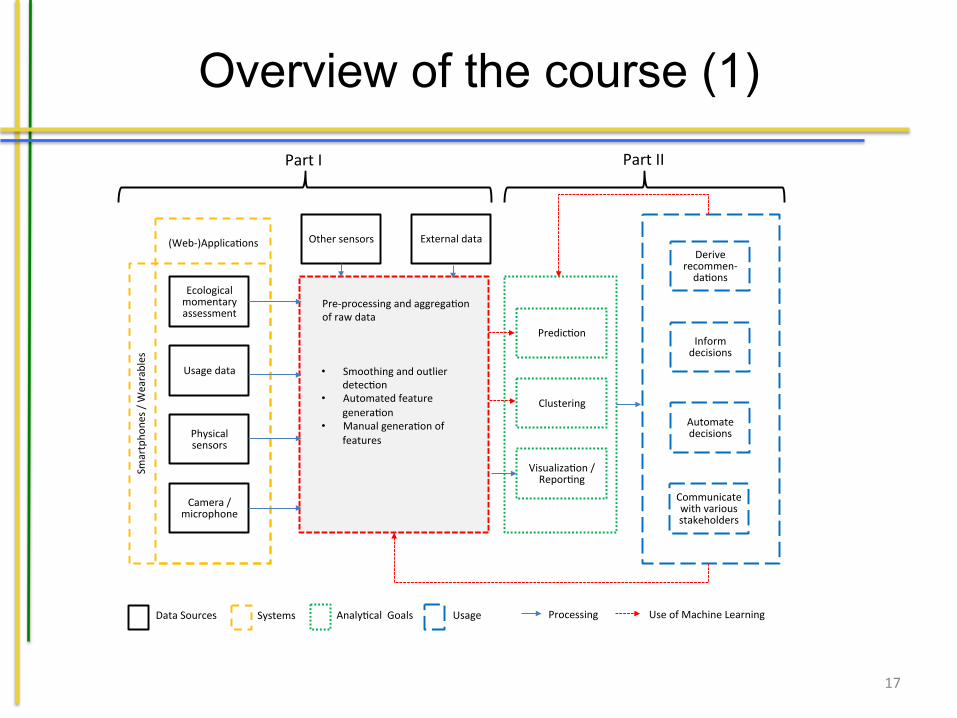
1.5 Overview of the book
Figure 1.1 shows an overview of the various elements deemed relevant for the quan-tified self in this book. In the figure, we see systems that measure and generatesensory data marked in yellow. The measurements can include data based on an-swers to questionnaires posed to the user in a certain context (ecological momen-tary assessment), usage data of a device, data from physical sensors (think of anaccelerometer), and audiovisual information obtained through a camera or micro-phone. Additional sensors not part of the smartphone or wearables can also providedata, for instance indoor positioning sensors. Finally, external data can be included,for example weather forecasts, or the medical history. To use all of this data weneed to do some pre-processing before we can actually perform the machine learn-ing tasks we aim to do. This is shown in the red box. Smoothing of the data, handlingmissing values and outliers, and the generation of useful features are the core partshere. Using the resulting dataset, we can perform an analysis: we can create mod-els that can be used for prediction of unknown values using a variety of machinelearning techniques; we can detect interesting patterns and relations in the data (e.g.clusters), and can create visualizations to gain insights into the data. These analyt-ical goals are shown in the green box. Finally, we can start using the knowledgewe have gained (the blue box) by deriving recommendations, informing decisions,automating them and communicating with the various stakeholders (in the context
Overview of the course (1)
17
10 1 Introduction
of Bruce, think of Bruce himself, his therapist, etcetera). In accordance with thisoverview, this book has been divided into three main parts:
Smartpho
nes/W
earables
Usagedata
Ecologicalmomentaryassessment
(Web-)Applica<ons Othersensors
Physicalsensors
Camera/microphone
Externaldata
DataSources Systems
• Smoothingandoutlierdetec<on
• Automatedfeaturegenera<on
• Manualgenera<onoffeatures
Analy<calGoals
Predic<on
Deriverecommen-da<ons
Processing
Clustering
Visualiza<on/Repor<ng
Communicatewithvariousstakeholders
Informdecisions
Automatedecisions
Usage UseofMachineLearning
Pre-processingandaggrega<onofrawdata
PartI PartII
Fig. 1.1: Various elements relevant to make sense out of quantified self data.
• The first part covers the pre-processing of the data and derivation of features.We will start with explaining the basics of sensory data and introduce the datasetwe use as a case study throughout nearly all chapters. Next, we explain how tosmooth the data and remove obvious outliers. Finally, we will go into depth onthe extraction of useful features from the cleaned data.
• The second part explains all relevant machine learning techniques that can helpus to reach our analytical goals, and also allow us to ”close the loop”, i.e. helpus to use the outcomes of the analysis to support the user more effectively. Thefirst topic we will cover is the clustering of the data. Here, we will focus onclustering of the data of a single user, but also the clustering on a higher level,namely the clustering over different users. We will then elaborate on the the-oretical foundations behind supervised learning, and cover supervised machinelearning approaches, both those that exploit the temporal dimension of data andthose that do not. We conclude with an introduction of reinforcement learningtechniques that allow us to learn how to effectively intervene and support a userin achieving his or her goals.
• Finally, the third part is a discussion about avenues for future developments thatwe identify.
Overview of the course / the book (2)
18
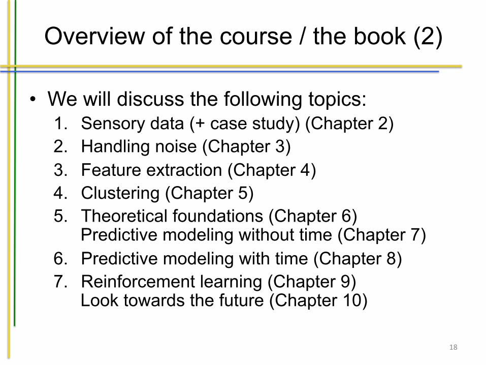
• We will discuss the following topics: 1. Sensory data (+ case study) (Chapter 2) 2. Handling noise (Chapter 3) 3. Feature extraction (Chapter 4) 4. Clustering (Chapter 5) 5. Theoretical foundations (Chapter 6)
Predictive modeling without time (Chapter 7) 6. Predictive modeling with time (Chapter 8) 7. Reinforcement learning (Chapter 9)
Look towards the future (Chapter 10)